PRIMORDIAL GRAVITATIONAL WAVES AND COSMIC MICROWAVE BACKGROUND RADIATION

Abstract

This is a summary of presentations delivered at the OC1 parallel session “Primordial Gravitational Waves and the CMB” of the $12^{\rm th}$ Marcel Grossmann meeting in Paris, July 2009. The reports and discussions demonstrated significant progress that was achieved in theory and observations. It appears that the existing data provide some indications of the presence of gravitational wave contribution to the CMB anisotropies, while ongoing and planned observational efforts are likely to convert these indications into more confident statements about the actual detection.

1 Introduction

Here, we report on presentations and discussions that took place at the OC1 parallel session entitled “Primordial Gravitational Waves and the CMB”. The programme was designed to include both theoretical and observational results. The electronic versions of some of the talks delivered at this session are available at the MG12 website [1]. We shall start from the overall framework of this session and motivations for studying the primordial (relic) gravitational waves.

Primordial gravitational waves (PGWs) are necessarily generated by a strong variable gravitational field of the very early Universe [2]. The existence of relic grtavitational waves relies only on the validity of basic laws of general relativity and quantum mechanics. Specifically, the generating mechanism is the superadiabatic (parametric) amplification of the waves’ zero-point quantum oscillations. In contrast to other known massless particles, the coupling of gravitational waves to the external (“pump”) gravitational field is such that they could be classically amplified or quantum-mechanically generated by the gravitational field of a homogeneous isotropic FLRW (Friedmann-Lemaitre-Robertson-Walker) universe. Under certain extra conditions the same applies to the primordial density perturbations. The PGWs are the cleanest probe of the physical conditions in the early Universe right down to the limits of applicability of currently available theories, i.e. the Planck density $\rho_{\rm Pl}=c^{5}/G^{2}\hbar\approx 10^{94}{\rm g}/{\rm cm}^{3}$ and the Planck size $l_{\rm Pl}=(G\hbar/c^{3})^{1/2}\approx 10^{-33}{\rm cm}$.

The amount and spectral content of the PGWs field depend on the evolution of the cosmological scale factor $a(\eta)$ representing the gravitational pump field. The theory was applied to a variety of $a(\eta)$, including those that are now called inflationary models [2, 3, 4]. If the exact $a(\eta)$ were known in advance from some fundamental “theory-of-everything”, we would have derived the properties of the today’s signal with no ambiguity. In the absence of such a theory, we have to use the available partial information in order to reduce the number of options. The prize is very high - the actual detection of a particular background of PGWs will provide us with a unique clue to the birth of the Universe and its very early dynamical behaviour.

To be more specific, let us put PGWs in the context of a complete cosmological theory hypothesizing that the observed Universe has come to the existence with near-Planckian energy density and size (see papers [5, 6] and references therein). It seems reasonable to conjecture that the embryo Universe was created by a quantum-gravity or by a “theory-of-everything” process in a near-Planckian state and then started to expand. (If you think that the development of a big universe from a tiny embryo is arrant nonsense, you should recollect that you have also developed from a single cell of microscopic size. Analogy proposed by the biophysicist E. Grishchuk.) The total energy, including gravity, of the emerging classical configuration was likely to be zero then and remains zero now.

In order for the natural hypothesis of spontaneous birth of the observed Universe to bring us anywhere near our present state characterized by $\rho_{p}=3H_{0}^{2}/8\pi G\approx 10^{-29}{\rm g}/{\rm cm}^{3}$ and $l_{p}=500l_{H}$ (which is the minimum size of the present-day patch of homogeneity and isotropy, as follows from observations [7]) the newly-born Universe needs a significant ‘primordial kick’. During the kick, the size of the Universe (or, better to say, the size of our patch of homogeneity and isotropy) should increase by about 33 orders of magnitude without losing too much of the energy density of whatever substance that was there, or maybe even slightly increasing this energy density at the expence of the energy density of the gravitational field. This process is graphically depicted in Fig. 1 (adopted from the paper [6]). The present state of the accessible Universe is marked by the point P, the birth of the Universe is marked by the point B. If the configuration starts at the point B and then expands according to the usual laws of radiation-dominated and matter-dominated evolution (blue curve), it completely misses the desired point P. By the time the Universe has reached the size $l_{p}$, the energy density of its matter content would have dropped to the level many orders of magnitude lower than the required $\rho_{p}$. The only way to reach P from B is to assume that the newly-born Universe has experienced a primordial kick allowing the point of evolution to jump over from the blue curve to the black curve.

If we were interested only in the zero-order approximation of homogeneity and isotropy, there would be many evolutionary paths equally good for connecting the points B and P. However, in the next-order approximations, which take into account the inevitable quantum-mechanical generation of cosmological perturbations, the positioning and form of the transition curve in Fig. 1 become crucial. The numerical value of the Hubble parameter $H$ (related to the energy density of matter driving the kick, as shown on the vertical axis of the figure) determines the numerical level of amplitudes of the generated cosmological perturbations, while the shape of the transition curve determines the shape of the primordial power spectrum.

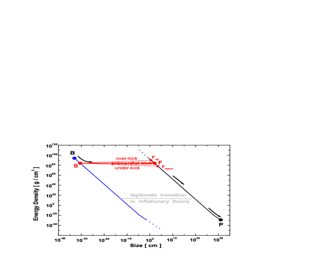
Figure 1: A primordial kick is required in order to reach the present state of the Universe P from the birth event B. Red lines describe possible transitions that would be accompanied by the generated cosmological perturbations of observationally necessary level and spectral shape [6]. The “legitimate transition in inflationary theory” is an evolution allowed by the incorrect (inflationary) formula for density perturbations. See explanations in Sec.3.2 below.

The simplest assumption about the initial kick is that its entire duration was characterized by a single power-law scale factor [2]

$$a(\eta)=l_{o}|\eta|^{1+\beta},$$ (1)

where $l_{o}$ and $\beta$ are constants, and $\beta<-1$. In this power-law case, the gravitational pump field is such that the generated primordial metric power spectra (primordial means considered for wavelengths longer than the Hubble radius at the given moment of time), for both gravitational waves and density perturbations, have the universal power-law dependence on the wavenumber $n$:

$$h^{2}(n)\propto n^{2(\beta+2)}.$$ (2)

It is common to write these metric power spectra separately for gravitational waves (gw) and density perturbations (dp):

$$h^{2}(n)~{}({\rm gw})=B_{t}^{2}n^{n_{t}},~{}~{}~{}~{}~{}h^{2}(n)~{}({\rm dp})=B_{s}^{2}n^{n_{s}-1}.$$ (3)

According to the theory of quantum-mechanical generation of cosmological perturbations (for a review, see [3]), the spectral indices are approximately equal, $n_{s}-1=n_{t}=2(\beta+2)$, and the amplitudes $B_{t}$ and $B_{s}$ are of the order of magnitude of the ratio $H_{i}/H_{\rm Pl}$, where $H_{i}\sim c/l_{o}$ is the characteristic value of the Hubble parameter $H$ during the kick. The straight lines in Fig. 1 symbolize the power-law kicks (1). They generate primordial spectra with constant spectral indices throughout all wavelenghts. In particular, any horizontal line describes an interval of de Sitter evolution, $\beta=-2$, ${\dot{H}}=0$, $H=const$. (Initial kick driven by a scalar field is appropriately called inflation: dramatic increase in size with no real change in purchasing power, i.e. in matter energy density.) The gravitational pump field of a de Sitter kick transition generates perturbations with flat (scale-independent) spectra $n_{s}-1=n_{t}=0$. The red horizontal line shown in Fig. 1 corresponds to $H_{i}/H_{\rm Pl}\approx 10^{-5}$ and the generated primordial amplitudes $B_{t}\approx B_{s}\approx 10^{-5}$. In numerical calculations, the primordial metric power spectra are usually parameterized by

$$P_{t}(k)=A_{t}(k/k_{0})^{n_{t}},~{}~{}P_{s}(k)=A_{s}(k/k_{0})^{n_{s}-1},$$ (4)

where $k_{0}=0.002$Mpc^-1.

Although the assumption of a single piece of power-law evolution (1) is simple and easy to analyze, the reality could be more complicated and probably was more complicated (see the discussion of WMAP data in Sec.3.2). A less simplistic kick can be approximated by a sequence of power-law evolutions, and then the primordial power spectra will consist of a sequence of power-law intervals.

The amplitudes of generated cosmological perturbations are large at long wavelengths. According to the widely accepted assumption the observed anisotropies in the cosmic microwave background radiation (CMB) are caused by perturbations of quantum-mechanical origin. This assumption is partially supported by the observed “peak and dip” structure of the CMB angular power spectra. Presumably, this structure reflects the phenomenon of quantum-mechanical phase squeezing and standing-wave pattern of the generated metric fields [3]. The search for the relic gravitational waves is a goal of a number of current and future space-borne, sub-orbital and ground-based CMB experiments [8, 9, 10, 11, 12, 13, 14, 15, 16].

The CMB anisotropies are usually characterized by the four angular power spectra $C_{\ell}^{TT}$, $C_{\ell}^{EE}$, $C_{\ell}^{BB}$ and $C_{\ell}^{TE}$ as functions of the multipole number $\ell$. The contribution of gravitational waves to these power spectra has been studied, both analytically and numerically, in a number of papers [17, 18, 19, 20, 21]. The derivation of today’s CMB power spectra brings us to approximate formulas of the following structure [20]:

$$\begin{array}[]{l}C_{\ell}^{TT}=\int\frac{dn}{n}[h(n,\eta_{rec})]^{2}\left[F^{T}_{\ell}(n)\right]^{2},\\ C_{\ell}^{TE}=\int\frac{dn}{n}h(n,\eta_{rec})h^{\prime}(n,\eta_{rec})\left[F^{T}_{\ell}(n)F^{E}_{\ell}(n)\right],\\ C_{\ell}^{YY}=\int\frac{dn}{n}[h^{\prime}(n,\eta_{rec})]^{2}\left[F^{Y}_{\ell}(n)\right]^{2},~{}~{}~{}~{}{\rm where}~{}Y=E,B.\end{array}$$ (8)

In the above expressions, $[h(n,\eta_{rec})]^{2}$ and $[h^{\prime}(n,\eta_{rec})]^{2}$ are power spectra of the gravitational wave field and its first time-derivative. The spectra are taken at the recombination (decoupling) time $\eta_{rec}$. The functions $F^{X}_{\ell}(n)$ ($X=T,E,B$) take care of the radiative transfer of CMB photons in the presence of metric perturbations. To a good approximation, the power residing in the metric fluctuations at wavenumber $n$ translates into the CMB $TT$ power at the angular scales characterized by the multipoles $\ell\approx n$. Similar results hold for the CMB power spectra induced by density perturbations. Actual numerical calculations use equations more accurate than Eq. (8).

There are several differences between the CMB signals arising from density perturbations and gravitational waves. For example, gravitational waves produce B-component of polarization, while density perturbations do not [18]; gravitational waves produce negative TE-correlation at lower multipoles, while density perturbations produce positive correlation [3, 20, 22, 23, 24], and so on. However, it is important to realize that it is not simply the difference between zero and non-zero or between positive and negative that matters. (In any case, various noises and systematics will make this division much less clear cut.) What really matters is that the gw and dp sources produce different CMB outcomes, and they are in principle distinguishable, even if they both are non-zero and of the same sign. For example, if the parameters of density perturbations were precisely known from other observations, any observed deviation from the expected $TT$, $TE$ and $EE$ correlation functions could be attributed (in conditions of negligible noises) to gravitational waves. From this perspective, the identification of the PGWs signal goes well beyond the often stated goal of detecting the B-mode of polarization. In fact, as was argued in the talk by D. Baskaran, delivered on behalf of the group including also L. P. Grishchuk and W. Zhao, the $TT$, $TE$, and $EE$ observational channels could be much more informative than the $BB$ channel alone. Specifically for the Planck mission, the inclusion of other correlation functions, in addition to $BB$, will significantly increase the expected signal-to-noise ratio in the PGWs detection.

It is convenient to compare the gravitational wave signal in CMB with that induced by density perturbation. A useful measure, directly related to observations, is the quadrupole ratio $R$ defined by

$$R\equiv\frac{C_{\ell=2}^{TT}({\rm gw})}{C_{\ell=2}^{TT}({\rm dp})},$$ (9)

i.e. the ratio of contributions of gw and dp to the CMB temperature quadrupole. Another measure is the so-called tensor-to-scalar ratio $r$. This quantity is built from primordial power spectra (4):

$$r\equiv\frac{A_{t}}{A_{s}}.$$ (10)

Usually, one finds this parameter linked to incorrect (inflationary) statements. Concretely, inflationary theory substitutes (for “consistency”) its prediction of arbitrarily large amplitudes of density perturbations in the limit of models where spectral index $n_{s}$ approaches $n_{s}=1$ and $n_{t}$ approaches $n_{t}=0$ (horizontal transition lines in Fig. 1) by the claim that it is the amount of relic gravitational waves, expressed in terms of $r$, that should be arbitrarily small. (For more details, see Sec. 3.2.) However, if $r$ is defined by Eq.(10) without implying inflationary claims, one can use this parameter. Moreover, one can derive a relation between $R$ and $r$ which depends on the background cosmological model and spectral indices. For a rough comparison of results one can use $r\approx 2R$.

2 Overview of oral presentations

The OC1 session opened with the talk of Brian Keating, appropriately entitled “The Birth Pangs of the Big Bang in the Light of BICEP”. The speaker reported on the initial results from the Background Imaging of Cosmic Extragalactic Polarization (BICEP) experiment. The conclusions were based on data from two years of observation. For the first time, some meaningful limits on $r$ were set exclusively from the fact of (non)observation of the B-mode of polarization (see figure 2 adopted from Chiang et al. paper[25]). The author paid attention to various systematic effects and showed that they were smaller than the statistical errors. B. Keating explained how the BICEP’s design and observational strategies will serve as a guide for future experiments aimed at detecting primordial gravitational waves. In conclusion, it was stressed that a further $90\%$ increase in the amount of analyzed BICEP data is expected in the near future.

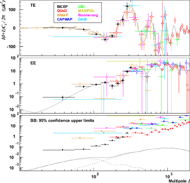
Figure 2: BICEPs TE, EE, and BB power spectra together with data from other CMB polarization experiments. Theoretical spectra from a CDM model with $r=0.1$ are shown for comparison. The BB curve is the sum of the gravitational wave and lensing components. At degree angular scales BICEPs constraints on $BB$ are the most powerful to date [25].

The next talk, delivered by Deepak Baskaran (co-authors: L. P. Grishchuk and W. Zhao), was entitled “Stable indications of relic gravitational waves in WMAP data and forecasts for the Planck mission”. D. Baskaran reported on the results of the likelihood analysis, performed by this group of authors, of the WMAP 5-year $TT$ and $TE$ data at lower multipoles. Obviously, in the center of their effort was the search for the presence of a gravitational wave signal [23, 24]. For the parameter $R$, the authors found the maximum likelihood value $R=0.23$, indicating a significant amount of gravitational waves. Unfortunately, this determination is surrounded by large uncertainties due to remaining noises. This means that the hypothesis of no gravitational waves, $R=0$, cannot be excluded yet with any significant confidence. The speaker compared these findings with the result of WMAP team, which found no evidence for gravitational waves. The reasons by which the gw signal can be overlooked in a data analysis were identified and discussed. Finally, D. Baskaran presented the forecasts for the Planck mission. It was shown that the stable indications of relic gravitational waves in the WMAP data are likely to become a certainty in the Planck experiment. Specifically, if PGWs are characterized by the maximum likelihood parameters found [23, 24] from WMAP5 data, they will be detected by Planck at the signal-to-noise level $S/N=3.65$, even under unfavorable conditions in terms of instrumental noises and foregrounds. (For more details along these lines, see sections below.)

The theoretical aspects of generation of CMB polarization and temperature anisotropies by relic gravitational waves were reviewed by Alexander Polnarev in the contribution “CMB polarization generated by primordial gravitational waves. Analytical solutions”. The author described the analytical methods of solving the radiative transfer equations in the presence of gravitational waves. This problem is usually tackled by numerical codes, but this approach foreshadows the ability of the researcher to understand the physical origin of the results. The analytical methods are a useful complement to numerical techniques. They allow one not only to explain in terms of the underlying physics the existing features of the final product, but also anticipate the appearance of new features when the physical conditions change. A. Polnarev showed how the problem of CMB anisotropies induced by gravitational waves can be reduced to a single integral equation. This equation can be further analyzed in terms of some integral and differential operators. Building on this technique, the author formulated analytical solutions as expansion series over gravitational wave frequency. He discussed the resonance generation of polarization and possible observational consequences of this effect.

An overview of the current experimental situation was delivered by Carrie MacTavish in the talk “CMB from space and from a balloon”. C. MacTavish focused on the interplay between experimental results from two CMB missions: the Planck satellite and the Spider balloon experiment. Spider is scheduled for flight over Australia in spring 2010 making measurements with 1600 detectors. The speaker emphasised the important combined impact of these two experiments on determination of cosmological parameters in general.

The ever increasing precision of CMB experiments warrants analysis of subtle observational effects inspired by the ideas from particle physics. The talk by Stephon Alexander “Can we probe leptogenesis from inflationary primordial birefringent gravitational waves” discussed a special mechanism of production of the lepton asymmetry with the help of cosmological birefringent gravitational waves. This mechanism was proposed in the recent paper [26]. The mechanism assumes that gravitational waves are generated in the presence of a CP violating component of the inflaton field that couples to a gravitational Chern-Simons term (Chern-Simons gravity). The lepton number arises via the gravitational anomaly in the lepton number current. As pointed out by the speaker, the participating gravitational waves should lead to a unique parity violating cross correlation in the CMB. S. Alexander discussed the viability of detecting such a signal, and concluded by analyzing the corresponding observational constraints on the proposed mechanism of leptogenesis.

Apart from being an arena for detecting relic gravitational waves, CMB is of course a powerful tool for cosmology in general. The final talk of the session, delivered by Grant Mathews (co-authors D. Yamazaki, K. Ichiki and T. Kajino), discussed the “Evidence for a primordial magnetic field from the CMB temperature and polarization power spectra”. This is an interesting subject as the magnetic fields are abundant in many astrophysical and cosmological phenomena. In particular, primordial magnetic fields could manifest themselves in the temperature and polarization anisotropies of the CMB. The speaker reported on a new theoretical framework for calculating CMB anisotropies along with matter power spectrum in the presence of magnetic fields with power-law spectra. The preliminary evidence from the data on matter and CMB power spectra on small angular scales suggest an upper and a lower limit on the strength of the magnetic field and its spectral index. It was pointed out that this determination might be the first direct evidence of the presence of primordial magnetic field in the era of recombination. Finally, the author showed that the existence of such magnetic field can lead to an independent constraint on the neutrino mass.

3 Analysis of WMAP data and outlook for Planck

Along the lines of the presentation by Baskaran et al, we review the results of the recent analysis of WMAP 5-year data. The results suggest the evidence, although still preliminary, that relic gravitational waves are present, and in the amount characterized by $R\approx 0.23$, This conclusion follows from the likelihood analysis of WMAP5 $TT$ and $TE$ data at lower multipoles $\ell\leq 100$. It is only within this range of multipoles that the power in relic gravitational waves is comparable with that in density perturbations, and gravitational waves compete with density perturbations in generating CMB temperature and polarization anisotropies. At larger multipoles, the dominant signal in CMB comes primarily from density perturbations.

3.1 Likelihood analysis of WMAP data

The analysis in papers [23, 24] was based on proper specification of the likelihood function. Since $TT$ and $TE$ data are the most informative in the WMAP5, the likelihood function was marginalized over the remaining data variables $EE$ and $BB$. In what follows $D_{\ell}^{TT}$ and $D_{\ell}^{TE}$ denote the estimators (and actual data) of the $TT$ and $TE$ power spectra. The joint pdf for $D_{\ell}^{TT}$ and $D_{\ell}^{TE}$ has the form

$$f(D_{\ell}^{TT},D_{\ell}^{TE})=n^{2}{x}^{\frac{n-3}{2}}\left\{2^{1+n}\pi\Gamma^{2}(\frac{n}{2})(1-\rho_{\ell}^{2})(\sigma_{\ell}^{T})^{2n}(\sigma_{\ell}^{E})^{2}\right\}^{-\frac{1}{2}}$$

$$\times\exp\left\{\frac{1}{1-\rho^{2}_{\ell}}\left(\frac{{\rho_{\ell}}{z}}{{\sigma_{\ell}^{T}}{\sigma_{\ell}^{E}}}-\frac{{z}^{2}}{2x{(\sigma_{\ell}^{E})^{2}}}-\frac{{x}}{2{(\sigma_{\ell}^{T})^{2}}}\right)\right\}.$$ (11)

This pdf contains the variables (actual data) $D_{\ell}^{XX^{\prime}}$ ($XX^{\prime}=TT,TE$) in quantities ${x}\equiv n(D_{\ell}^{TT}+N_{\ell}^{TT})$ and ${z}\equiv nD_{\ell}^{TE}$, where $N_{\ell}^{TT}$ is the temperature total noise power spectrum. The quantity $n=(2\ell+1)f_{\rm sky}$ is the number of effective degrees of freedom at multipole $\ell$, where $f_{\rm sky}$ is the sky-cut factor. $f_{\rm sky}=0.85$ for WMAP and $f_{\rm sky}=0.65$ for Planck. $\Gamma$ is the $Gamma$-function. The quantities $\sigma_{\ell}^{T}$, $\sigma_{\ell}^{E}$ and $\rho_{\ell}$, include theoretical power spectra $C_{\ell}^{XX^{\prime}}$ and contain the perturbation parameters $R$, $A_{s}$, $n_{s}$ and $n_{t}$, whose numerical values the likelihood analysis seeks to find.

The three free perturbation parameters $R$, $A_{s}$, $n_{s}$ ($n_{t}=n_{s}-1$) were determined by maximizing the likelihood function

$$\mathcal{L}\propto\prod_{\ell}f(D_{\ell}^{TT},D_{\ell}^{TE})$$

for $\ell=2...100$. The background cosmological model was fixed at the best fit $\Lambda$CDM cosmology [27]. The maximum likelihood (ML) values of the perturbation parameters (i.e. the best fit values), were found to be

$$R=0.229,~{}~{}~{}n_{s}=1.086,~{}~{}~{}A_{s}=1.920\times 10^{-9}$$ (12)

and $n_{t}=0.086$. The region of maximum likelihood was probed by 10,000 sample points using MCMC method. The projections of all 10,000 points on 2-dimensional planes $R-n_{s}$ and $R-A_{s}$ are shown in Fig. 3.

The samples with relatively large values of the likelihood (red, yellow and green colors) are concentrated along the curve, which projects into approximately straight lines (at least, up to $R\approx 0.5$):

$$n_{s}=0.98+0.46R,~{}~{}~{}~{}~{}A_{s}=(2.27-1.53R)\times 10^{-9}.$$ (13)

These combinations of parameters $R,n_{s},A_{s}$ produce roughly equal responses in the CMB power spectra. The best fit model (12) is a particular point on these lines, $R=0.229$. The family of models (13) is used in Sec.3.3 for setting the expectations for the Planck experiment.

The marginalized 2-dimensional and 1-dimensional distributions are plotted in Fig. 4 and Fig. 5, respectively. The ML values for the 1-dimensional marginalized distributions and their $68.3\%$ confidence intervals are given by

$$R=0.266\pm 0.171,~{}~{}n_{s}=1.107^{+0.087}_{-0.070},~{}~{}A_{s}=(1.768^{+0.307}_{-0.245})\times 10^{-9}.$$ (14)

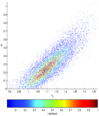
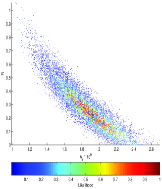
Figure 3: The projection of 10,000 samples of the 3-dimensional likelihood function onto the $R-n_{s}$ (left panel) and $R-A_{s}$ (right panel) planes. The color of an individual point in Fig. 3 signifies the value of the 3-dimensional likelihood of the corresponding sample. The black $+$ indicates the parameters listed in (12). Figure adopted from Zhao et al [24].

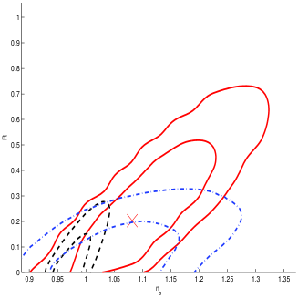
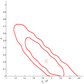
Figure 4: The ML points (red $\times$) and the $68.3\%$ and $95.4\%$ confidence contours (red solid lines) for 2-dimensional likelihoods: $R-n_{s}$ (left panel) and $R-A_{s}$ (right panel). In the left panel, the WMAP confidence contours are also shown for comparison. Figure adopted from Zhao et al [24].

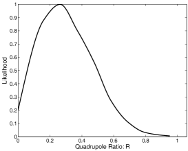
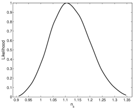
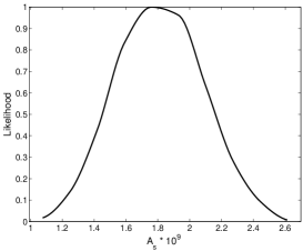
Figure 5: 1-dimensional likelihoods for $R$ (left), $n_{s}$ (middle) and $A_{s}$ (right). Figure adopted from Zhao et al [24].

The derived results allow one to conclude that the maximum likelihood value of $R$ persistently indicates a significant amount of relic gravitational waves, even if with a considerable uncertainty. The $R=0$ hypothesis (no gravitational waves) appears to be away from the $R=0.229$ model at about $1\sigma$ interval, or a little more, but not yet at a significantly larger distance. The spectral indices $n_{s},n_{t}$ persistently point out to the ‘blue’ shape of the primordial spectra, i.e. $n_{s}>1,n_{t}>0$, in the interval of wavelengths responsible for the analyzed multipoles $\ell\leq\ell_{max}=100$. This puts in doubt the (conventional) scalar fields as a possible driver for the initial kick, because the scalar fields cannot support $\beta>-2$ and, consequently, cannot support $n_{s}>1,n_{t}>0$.

3.2 How relic gravitational waves can be overlooked in the likelihood analysis of data

The results of this analysis differ from the conclusions of WMAP team [27]. The WMAP team found no evidence for gravitational waves and arrived at a ‘red’ spectral index $n_{s}=0.96$. The WMAP findings are symbolized by black dashed and blue dash-dotted contours in Fig. 4. It is important to discuss the likely reasons for these disagreements.

Two main differences in the data analysis are as follows. First, the present analysis is restricted only to multipoles $\ell\leq 100$ (i.e. to the interval in which there is any chance of finding gravitational waves), whereas the WMAP team uses the data from all multipoles up to $\ell\sim 1000$, keeping spectral indices constant in the entire interval of participating wavelengths (thus making the uncertainties smaller by increasing the number of included data points which have nothing to do with gravitational waves). Second, in the current work, the relation $n_{t}=n_{s}-1$ implied by the theory of quantum-mechanical generation of cosmological perturbations is used, whereas WMAP team uses the inflationary ‘consistency relation’ $r=-8n_{t}$, which automatically sends $r$ to zero when $n_{t}$ approaches zero.

It is important to realize that the inflationary ‘consistency relation’

$$r=16\epsilon=-8n_{t}$$

is a direct consequence of the single contribution of inflationary theory to the subject of cosmological perturbations, which is the incorrect formula for the power spectrum of density perturbations, containing the “zero in the denominator” factor:

$$P_{s}\approx\frac{1}{\epsilon}\left(\frac{H}{H_{Pl}}\right)^{2}.$$

The “zero in the denominator” factor $\epsilon$ is $\epsilon\equiv-{\dot{H}}/{H^{2}}$. This factor tends to zero in the limit of standard de Sitter inflation ${\dot{H}}=0$ (any horizontal line in Fig. 1) independently of the curvature of space-time and strength of the generating gravitational field characterized by $H$. To make the wrong theory look “consistent”, inflationary model builders push $H/H_{Pl}$ down, whenever $\epsilon$ goes to zero (for example, down to the level marked by the minutely inclined line “legitimate transition in inflationary theory” in Fig. 1), thus keeping $P_{s}$ at the observationally required level and making the amount of relic gravitational waves arbitrarily small. In fact, the most advanced inflationary theories based on strings, branes, loops, tori, monodromies, etc. predict the ridiculously small amounts of gravitational waves, something at the level of $r\approx 10^{-24}$, or so. [There is no doubt, there will be new inflationary theories which will predict something drastically different. Inflationists are good at devising theories that only mother can love, but not at answering simple physical questions such as quantization of a cosmological oscillator with variable frequency. For a more detailed criticism of inflationary theory, see Grishchuk[3].] Obviously, the analysis in papers [23, 24] does not use the inflationary theory.

Baskaran et al concluded that in the conditions of relatively noisy WMAP data it was the assumed constancy of spectral indices in a broad spectrum [27] that was mostly responsible for the strong dissimilarity of data analysis results with regard to gravitational waves. Having repeated the same analysis of data in the adjacent interval of multipoles $101\leq\ell\leq 220$, the authors of paper [24] found a somewhat different (smaller) spectral index $n_{s}$ in this interval. They came to the conclusion that the hypothesis of strictly constant spectral indices (perfectly straight lines in Fig. 1) should be abandoned. It is necessary to mention that the constancy of $n_{s}$ over the vast region of wavenumbers, or possibly a simple running of $n_{s}$, is a usual assumption in a number of works [27, 28, 29].

It is now clear why it is dangerous, in the search for relic gravitational waves, to include data from higher multipoles, and especially assuming a strictly constant spectral index $n_{s}$. Although the higher multipole data have nothing to do with gravitational waves, they bring $n_{s}$ down. If one postulates that $n_{s}$ is one and the same constant at all $\ell$’s, this additional ‘external’ information about $n_{s}$ affects uncertainty about $R$ and brings $R$ down. This is clearly seen, for example, in the left panel of Fig. 4. The localization of $n_{s}$ near, say, the line $n_{s}=0.96$ would cross the solid red contours along that line and would enforce lower, or zero, values of $R$. However, as was shown [24], $n_{s}$ is sufficiently different even at the span of the two neighbouring intervals of $\ell$’s, namely $2\leq\ell\leq 100$ and $101\leq\ell\leq 220$. These considerations, as for how relic gravitational waves can be overlooked in a data analysis, have general significance and will be applicable to any CMB data.

3.3 Forecasts for the Planck mission

The final part of the presentation by Baskaran et al dealt with forecasts for the recently launched Planck satellite [8]. The ability of a CMB experiment to detect gravitational waves is characterized by the signal-to-noise ratio defined by [23, 24]

$$S/N\equiv R/\Delta R,$$ (15)

where the numerator is the “true” value of the parameter $R$ (its ML value or the input value in a numerical simulation) while $\Delta R$ in the denominator is the expected uncertainty in determination of $R$ from the data.

In formulating the observational expectations, all of the available information channels (i.e. $TT$, $TE$, $EE$ and $BB$ correlation functions) were taken into account. The calculations were performed using the Fisher matrix formalism. The total uncertainty entering the Fisher matrix calculations is comprised of instrumental and foreground noises [8, 30, 24] as well as the statistical uncertainty of the inherently random signal under discussion. The possibility of partial removal of contamination arising from foreground sources was quantified by the residual noise factor $\sigma^{\rm fg}$. The three considered cases included $\sigma^{\rm fg}=1$ (no foreground removal), $\sigma^{\rm fg}=0.1$ ($10\%$ residual foreground noise) and $\sigma^{\rm fg}=0.01$ ($1\%$ residual foreground noise). In order to gauge the worst case scenario, the ‘pessimistic’ case was added. It assumes $\sigma^{\rm fg}=1$ and the instrumental noise at each frequency $\nu_{i}$ four times larger than the nominal value reported by the Planck team. This increased noise is meant to mimic the situation where it is not possible to get rid of various systematic effects [31], the $E$-$B$ mixing [32], cosmic lensing [33], etc. which all affect the $BB$ channel.

The total $S/N$ for one parameter family of models defined by the large WMAP5 likelihoods (13) is plotted in Fig. 6. This graph is based on the conservative assumption that all unknown parameters $R$, $n_{s}$ and $A_{s}$ are evaluated from one and the same dataset. Four options are depicted: $\sigma^{\rm fg}=0.01,0.1,1$ and the pessimistic case. The results for the ML model (12) are given by the intersection points along the vertical line $R=0.229$. Specifically, $S/N=6.69,~{}6.20,~{}5.15$ for $\sigma^{\rm fg}=0.01,~{}0.1,~{}1$, respectively. The good news is that even in the pessimistic case one gets $S/N>2$ for $R>0.11$, and the Planck satellite will be capable of seeing the ML signal $R=0.229$ at the level $S/N=3.65$.

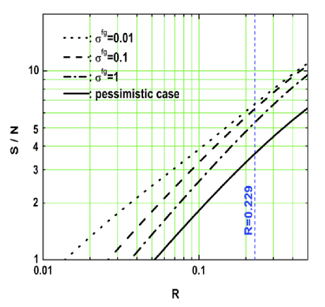
Figure 6: The $S/N$ as a function of $R$. Figure adopted from Zhao et al [24].

It is important to treat separately the contributions to the total signal-to-noise ratio supplied by different information channels and different individual multipoles. The $(S/N)^{2}$ calculated for three combinations of channels, $TT+TE+EE+BB$, $TT+TE+EE$ and $BB$ alone, is shown in Fig. 7. Four panels describe four noise models: $\sigma^{\rm fg}=0.01,~{}0.1,~{}1$ and the pessimistic case. Surely, the combination $TT+TE+EE+BB$ is more sensitive than any of the other two, i.e. $TT+TE+EE$ and $BB$ alone. For example, in the case $\sigma^{\rm fg}=0.1$ the use of all correlation functions ensures $S/N$ which is $\sim 50\%$ greater than $BB$ alone and $\sim 30\%$ greater than $TT+TE+EE$. The situation is even more dramatic in the pessimistic case. The ML model (12) can be barely seen through the $B$-modes alone, because the $BB$ channel gives only $S/N=1.75$, whereas the use of all of the correlation functions can provide a confident detection with $S/N=6.48$. Comparing $TT+TE+EE$ with $BB$ one can see that the first method is better than the second, except in the case when $\sigma^{\rm fg}=0.01$ and $R$ is small ($R<0.16$). In the pessimistic case, the role of the $BB$ channel is so small that the $TT+TE+EE$ method provides essentially the same sensitivity as all channels $TT+TE+EE+BB$ together.

Figure 7: The $S/N$ for different combinations of the information channels, $TT+TE+EE+BB$, $TT+TE+EE$ and $BB$. Figure adopted from Zhao et al [24].

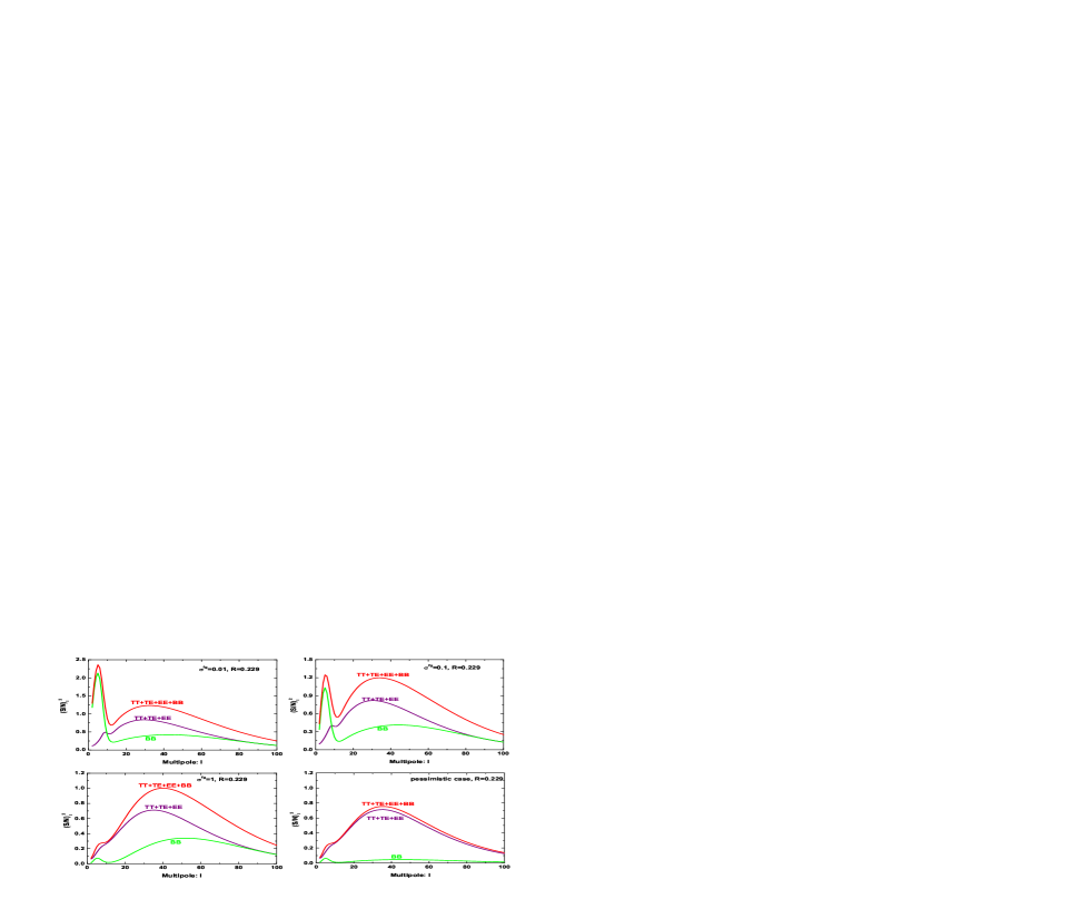
Figure 8: The individual $(S/N)_{\ell}^{2}$ as functions of $\ell$ for different combinations of information channels and different levels of foreground contamination. Calculations are done for the ML model (12) with $R=0.229$. Figure adopted from Zhao et al [24].

Finally, Fig. 8 shows the contributions to the total signal-to-noise ratio from individual multipoles. It can be seen that a very deep foreground cleaning, $\sigma^{\rm fg}=0.01$, makes the very low (reionization) multipoles $\ell\lesssim 10$ the major contributors to the total $(S/N)^{2}$, and mostly in the $BB$ channel. However, for large $\sigma^{\rm fg}=0.1,~{}1$, and especially in the pessimistic case (see the lower right panels in Fig. 8), the ability of the $BB$ channel becomes very degraded at all $\ell$’s. At the same time, as Fig. 8 illustrates, the $\ell$-decomposition of $(S/N)^{2}$ for $TT+TE+EE$ combination depends only weakly on the level of $\sigma^{\rm fg}$. Furthermore, in this method, the signal to noise curves generally peak at $\ell\sim(20-60)$. Therefore, it will be particularly important for Planck mission to avoid excessive noises in this region of multipoles.

4 Conclusions

In general, the OC1 parallel session was balanced and covered both theoretical and experimental aspects of primordial gravitational waves and the CMB. Thanks to excellent contributions of all participants, this subject received a new momentum. Hopefully, new observations and theoretical work will bring conclusive results in the near future.

References

- [1] Marcel Grossmann Meeting website, http://www.icra.it/MG/mg12/en.
- [2] L. P. Grishchuk, Zh. Eksp. Teor. Fiz. 67, 825 (1974) [Sov. Phys. JETP 40, 409 (1975)]; Ann. N. Y. Acad. Sci 302, 439 (1977); Pis’ma Zh. Eksp. Teor. Fiz. 23, 326 (1976) [JETP Lett. 23, 293 (1976)]; Usp. Fiz. Nauk 121, 629 (1977) [Sov. Phys. Usp. 20, 319 (1977)].
- [3] L. P. Grishchuk, Discovering Relic Gravitational Waves in Cosmic Microwave Background Radiation, Chapter in the book “General Relativity and John Archibald Wheeler”, edited by I. Ciufolini and R. Matzner, (Springer, New York, 2010), [arXiv:0707.3319].
- [4] A. A. Starobinsky, JETP Lett. 30, 682 (1979).
- [5] Ya. B. Zeldovich, Pis’ma JETP 7, 579 (1981); L. P. Grishchuk and Ya. B. Zeldovich, in Quantum Structure of Space and Time, Eds. M. Duff and C. Isham, (Cambridge University Press, Cambridge, 1982), p. 409; Ya. B. Zeldovich, Cosmological field theory for observational astronomers, Sov. Sci. Rev. E Astrophys. Space Phys. Vol. 5, pp. 1-37 (1986) (http://nedwww.ipac.caltech.edu/level5/Zeldovich/Zel_contents.html); A. Vilenkin, in “The Future of Theoretical Physics and Cosmology”, Eds. G. W. Gibbons, E. P. S. Shellard and S. J. Rankin (Cambridge University Press, 2003).
- [6] L. P. Grishchuk, Space Science Reviews 148, 1-4, 315 (2009) [arXiv:0903.4395].
- [7] L. P. Grishchuk and Ya. B. Zeldovich. Astron. Zh. 55, 209 (1978) [Sov. Astron. 22, 125 (1978)]; L. P. Grishchuk. Phys. Rev. D 45, 4717 (1992).
- [8] Planck Collaboration, The Science Programme of Planck [arXiv:astro-ph/0604069].
- [9] M. R. Nolta et al., Astrophys. J. Suppl. 180, 296 (2009).
- [10] B. G. Keating et al., in Polarimetry in Astronomy, edited by Silvano Fineschi, Proceedings of the SPIE, 4843 (2003).
- [11] C. Pryke et al., QUaD collaboration, Astrophys. J. 692, 1247 (2009).
- [12] A. C. Taylor, Clover Collaboration, New Astron. Rev. 50, 993 (2006).
- [13] D. Samtleben, arXiv:0806.4334.
- [14] P. Oxley et al., Proc. SPIE Soc. Opt. Eng. 5543, 320 (2004).
- [15] B. P. Crill et al., arXiv:0807.1548.
- [16] D. Baumann et al., AIP Conf. Proc. 1141, 10 (2009).
- [17] R. K. Sachs and A. M. Wolfe, Astrophys. J. 147, 73 (1967); L. P. Grishchuk and Ya. B. Zel’dovich, Soviet Astronomy 22, 125 (1978); V. A. Rubakov, M. V. Sazhin, A. V. Veryaskin, Phys. Lett. B 115, 189 (1983); A. Polnarev, Sov. Astron. 29, 6 (1985); A. A. Starobinskii, Pis’ma Astron. Zh. 11, 323 (1985); D. Harari and M. Zaldarriaga, Phys. Lett. B 310, 96 (1993); L. P. Grishchuk, Phys. Rev. Lett. 70, 2371 (1993). R. Crittenden et al., Phys. Rev. Lett. 71, 324 (1993); R. A. Frewin, A. G. Polnarev and P. Coles, Mon. Not. R. Astron. Soc. 266, L21 (1994).
- [18] M. Zaldariaga and U. Seljak, Phys. Rev. D 55, 1830 (1997); M. Kamionkowski, A. Kosowsky and A. Stebbins, Phys. Rev. D 55, 7368 (1997).
- [19] J. R. Pritchard and M. Kamionkowski, Ann. Phys. (N.Y.) 318, 2 (2005); W. Zhao and Y. Zhang, Phys. Rev. D 74, 083006 (2006); T. Y. Xia and Y. Zhang, Phys. Rev. D 78, 123005 (2008).
- [20] D. Baskaran, L. P. Grishchuk and A. G. Polnarev, Phys. Rev. D 74, 083008 (2006).
- [21] B. G. Keating, A. G. Polnarev, N. J. Miller and D. Baskaran, Int. J. Mod. Phys. A 21, 2459 (2006); R. Flauger and S. Weinberg, Phys. Rev. D 75, 123505 (2007); Y. Zhang, W. Zhao, X. Z. Er, H. X. Miao and T. Y. Xia, Int. J. Mod. Phys. D 17, 1105 (2008).
- [22] A. G. Polnarev, N. J. Miller and B. G. Keating, Mon. Not. R. Astron. Soc. 386, 1053 (2008); N. J. Miller and B. G. Keating and A. G. Polnarev, arXiv:0710.3651.
- [23] W. Zhao, D. Baskaran and L. P. Grishchuk, Phys. Rev. D 79, 023002 (2009).
- [24] W. Zhao, D. Baskaran and L. P. Grishchuk, Phys. Rev. D 80, 083005 (2009).
- [25] H. C. Chiang et al., Astrophys. J. 711, 1123 (2010).
- [26] S. H. Alexander, M. E. Peskin, M. M. Sheikh-Jabbari, Phys. Rev. Lett. 96, Issue 8, 081301 (2006).
- [27] E. Komatsu et al., Astrophys. J. Suppl. 180, 330 (2009).
- [28] e.g. A. Lewis, Phys. Rev. D 78, 023002 (2008); J. Q. Xia, H. Li, G. B. Zhao and X. M. Zhang, Phys. Rev. D 78, 083524 (2008); L. P. L. Colombo, E. Pierpaoli and J. R. Pritchard, arXiv:0811.2622.
- [29] W. Zhao, Phys. Rev. D 79, 063003 (2009); W. Zhao and D. Baskaran, Phys. Rev. D 79, 083003 (2009).
- [30] J. Dunkely et al., AIP Conf. Proc. 1141, 222 (2009).
- [31] W. Hu, M. M. Hedman and M. Zaldarriaga, Phys. Rev. D 67, 043004 (2003); D. O’Dea, A. Challinor and B. R. Johnson, Mon. Not. R. Astron. Soc. 376, 1767 (2007); M. Shimon, B. Keating, N. Ponthieu and E. Hivon, Phys. Rev. D 77, 083003 (2008).
- [32] A. Lewis, A. Challinor, and N. Turok, Phys. Rev. D 65, 023505 (2001); M. L. Brown, P. G. Castro, and A. N. Taylor, Mon. Not. R. Astron. Soc. 360, 1262 (2005); A. de Oliveira-Costa and M. Tegmark, Phys. Rev. D 74, 023005 (2006).
- [33] M. Zaldarriaga and U. Seljak, Phys. Rev. D 58, 023003 (1998); W. Hu, Phys. Rev. D 62, 043007 (2000).