811
J. de la Cruz Rodríguez
Observation and analysis of chromospheric magnetic fields
Abstract
The solar chromosphere is a vigorously dynamic region of the sun, where waves and magnetic fields play an important role. To improve chromospheric diagnostics, we present new observations in Ca II 8542 carried out with the SST/CRISP on La Palma, working in full-Stokes mode. We measured Stokes line profiles in active regions. The line profiles observed close to the solar limb show signals in all four Stokes parameters, while profiles observed close to disk center only show signals above the noise level in Stokes I and V. We used the NLTE inversion code ’NICOLE’ to derive atmospheric parameters in umbral flashes present in a small round sunspot without penumbra.
keywords:
Line: profiles – polarization – Techniques: polarimetric – Sun: chromosphere – Sun: magnetic fields1 Introduction
The magnetic structure of the solar chromosphere is currently the subject of intense computational and observational research. Numerical MHD simulations have improved in the last few years, becoming more and more realistic, i.e, Wedemeyer et al. (2004), Leenaarts et al. (2007) and Martínez-Sykora et al. (2009). Unfortunately, progress on the observational side has arguably been somewhat slower. The few optical spectral lines probing the chromosphere are typically characterized by:
-
1.
A vast formation range, from the photosphere to the chromosphere.
-
2.
NLTE.
-
3.
A weak polarization signal (especially in Q and U).
-
4.
A large spectral width.
Inversion codes have been commonly used to derive atmospheric parameters, usually assuming LTE or considering a Milne-Eddington atmosphere. However, this approximation cannot be used for modeling chromospheric lines, such as the Ca II infrared triplet. A method for NLTE inversions of Zeeman-induced Stokes profiles was described by Socas-Navarro et al. (2000b) and used in a study by Pietarila et al. (2007) of slit-based spectroscopic observations. The development of new instrumentation at large aperture telescopes (like SST/CRISP, DST/IBIS, VTT/TESOS) has made it possible to observe the chromosphere with very high spatial and temporal resolution. Here, we present inversions of chromospheric full-Stokes CRISP data.
2 The chromosphere observed with CRISP in 854.2 nm
CRISP is a Fabry-Pérot filter consisting of two etalons mounted in tandem. The rapid tuning ability in combination with two Liquid Crystal Variable Retarders allow for full-Stokes scanning of spectral line profiles. The transmission profile of the instrument at 8542 Å has a FWHM of 111 mÅ. The Ca II IR lines have a large formation range: the wings of the line are formed in the photosphere, while the inner core is formed in the lower chromosphere. Therefore, the features observed in the core of the line show significant changes on time scales of 3–5 seconds, whereas the features in the wings, showing the usual photospheric granulation pattern, evolve much slower ( 25 seconds). As with any Fabry-Perot instrument, there is a trade-off between cadence, sensitivity and number of wavelengths. The datasets were processed using MOMFBD (van Noort et al., 2005). It is important to note that our observations of active regions show similar chromospheric structures to those seen in H.
2.1 High resolution Umbral Flashes
In this study we present observations taken on 2008 June 12 at , with a cadence of 11 s per scan and covering a range of Å from line center. The dataset, shown in Fig. 1, includes a small sunspot without penumbra showing Umbral Flashes (UF, hereafter), one of the clearest examples of shock propagation in the Sun. Socas-Navarro et al. (2000a) report anomalous Zeeman profiles during the UF phase and propose a scenario in which this phenomenon may occur. Centeno et al. (2005) provide further evidence for the dual component scenario. Socas-Navarro et al. (2009) describe fine-scale structures in UF from Hinode Ca II H imaging, further supporting the idea of a highly structured umbral atmosphere. Our observations show the anomalous Stokes V profile during the UF phase in Fig. 3.

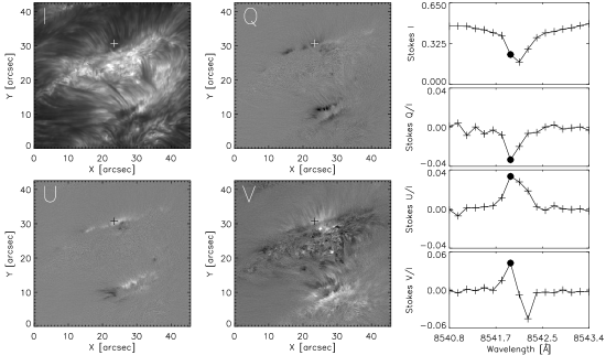
2.2 Active region at
Figure 2 shows an active region which encloses two small sunspots recorded on 2008 June 10 at . The Stokes images clearly show a linear polarization signal, while the Stokes V image suggests a very complicated magnetic field configuration. The circular polarization peaks around %, while the linear polarization measured in Stokes Q & U is (in most cases) lower than 4%. No inversions of this dataset were carried out.
3 NICOLE: the NLTE inversion code
We use the NLTE inversion code NICOLE, which assumes complete redistribution in frequencies and angles, and works with plane-parallel geometry. Line broadening produced by collisions with neutral H atoms follows the formulation described by Barklem et al. (2000). The code is based on the work presented in Socas-Navarro et al. (2000b). It solves the NLTE problem using the strategy described by Socas-Navarro & Trujillo Bueno (1997)
The inversions are initialized with a modified HSRA atmospheric model and the code uses CRISP’s non-Gaussian instrumental profile to degrade the synthetic spectra. Similar NLTE inversions are described in detail by Pietarila et al. (2007), but concerned quiet Sun and at a much lower spatial resolution.
We use NICOLE to invert the observations described in Sect. 2.1, with the aim of testing the code on CRISP observations for further analysis of the results. The weak Stokes signals, high image resolution, limited wavelength coverage and poor sampling of the line present a challenge for the analysis of such data. We carry out the inversions using only a single component atmosphere, even though UF probably require a multi-component treatment, and therefore, the results represent an average of multiple components. Figure 1 shows the selected target for the inversions, where the circle on the image marks an example pixel of which the inversion results are shown in Sect. 4.
4 Results
Unfortunately, NLTE inversions are computationally very expensive, making the analysis of time series of the whole field of view a time consuming task. Therefore, we have inverted spectra only along a line that crosses the pore for a 5 minutes time series. Figure 5 shows the time evolution of the spectrum of our example pixel. The UF starts around s and ends at s.

In the quiescent phase our target shows a traditional sunspot Stokes profile, with two Zeeman components in circular polarization with opposite signs. In the presence of an UF, the Stokes I profile shows an enhanced emission component on the blue side of the line core, which causes an apparent redshift of the line core, presented in Fig. 3. The shock has a strong signature in the Stokes V profile and makes the blue Zeeman component vanish. Figure 4 shows the atmospheric model obtained by inversions of the Stokes profiles of the example pixel during the quiescent (dashed line) and UF (solid line) phases. The UF is characterized by an upflow (negative velocity) in the higher layers of the model, compared to the quiescent phase. The density appears enhanced during the UF phase, and the measured magnetic field strength is lower due to the presence of the anomalous Stokes V profile. The azimuth and inclination of the magnetic field could not be derived from the Stokes data since the signal level in Stokes Q and U is too low. The round shape of the pore and the absence of a penumbra suggest that the magnetic field is mostly vertical, which for high values is roughly aligned with the line of sight, consistent with the low signal in Stokes Q and U.


5 Conclusions
We have reduced polarimetric CRISP observations of the Ca II 854.2 nm line and analyzed a small, round pore located at using an adapted version of the NLTE inversion code NICOLE. The code is not able to reproduce discontinuities as the model is smoothed with a spline fit during the inversion. Nevertheless, the shock leaves a clear fingerprint in the derived velocity, density and magnetic field strength. Since the observed Stokes V profile of this line is known to be properly described by Zeeman splitting in such a strong magnetic field, the spread in the magnetic field strength is probably mostly caused by noise. The amount of cross-talk between other thermodynamic parameters is still unknown and will be the subject of future research.
Acknowledgements.
This research project has been supported by a Marie Curie Early Stage Research Training Fellowship of the European Community’s Sixth Framework Program under contract number MEST-CT-2005-020395: The USO-SP International School for Solar Physics.References
- Barklem et al. (2000) Barklem, P. S., Piskunov, N., & O’Mara, B. J. 2000, A&AS, 142, 467
- Centeno et al. (2005) Centeno, R., Socas-Navarro, H., Collados, M., & Trujillo Bueno, J. 2005, ApJ, 635, 670
- Leenaarts et al. (2007) Leenaarts, J., Carlsson, M., Hansteen, V., & Rutten, R. J. 2007, A&A, 473, 625
- Martínez-Sykora et al. (2009) Martínez-Sykora, J., Hansteen, V., DePontieu, B., & Carlsson, M. 2009, ApJ, 701, 1569
- Pietarila et al. (2007) Pietarila, A., Socas-Navarro, H., & Bogdan, T. 2007, ApJ, 670, 885
- Socas-Navarro et al. (2009) Socas-Navarro, H., McIntosh, S. W., Centeno, R., de Wijn, A. G., & Lites, B. W. 2009, ApJ, 696, 1683
- Socas-Navarro & Trujillo Bueno (1997) Socas-Navarro, H. & Trujillo Bueno, J. 1997, ApJ, 490, 383
- Socas-Navarro et al. (2000a) Socas-Navarro, H., Trujillo Bueno, J., & Ruiz Cobo, B. 2000a, ApJ, 544, 1141
- Socas-Navarro et al. (2000b) Socas-Navarro, H., Trujillo Bueno, J., & Ruiz Cobo, B. 2000b, ApJ, 530, 977
- van Noort et al. (2005) van Noort, M., Rouppe van der Voort, L., & Löfdahl, M. G. 2005, Sol. Phys., 228, 191
- Wedemeyer et al. (2004) Wedemeyer, S., Freytag, B., Steffen, M., Ludwig, H., & Holweger, H. 2004, A&A, 414, 1121