Kondo effect in spin-orbit mesoscopic interferometers

Abstract

We consider a flux-threaded Aharonov-Bohm ring with an embedded quantum dot coupled to two normal leads. The local Rashba spin-orbit interaction acting on the dot electrons leads to a spin-dependent phase factor in addition to the Aharonov-Bohm phase caused by the external flux. Using the numerical renormalization group method, we find a splitting of the Kondo resonance at the Fermi level which can be compensated by an external magnetic field. To fully understand the nature of this compensation effect, we perform a scaling analysis and derive an expression for the effective magnetic field. The analysis is based on a tight-binding model which leads to an effective Anderson model with a spin-dependent density of states for the transformed lead states. We find that the effective field originates from the combined effect of Rashba interaction and magnetic flux and that it contains important corrections due to electron-electron interactions. We show that the compensating field is an oscillatory function of both the spin-orbit and the Aharonov-Bohm phases. Moreover, the effective field never vanishes due to the particle-hole symmetry breaking independently of the gate voltage.

I Introduction

Interference studies in solid-state mesoscopic interferometers provide most valuable information about scattering properties of artificial atoms (quantum dots).yac95 ; lev95 ; hac96 ; bru96 ; shu97 ; ji00 ; sig04 Interference takes place between electronic partial waves traveling along a nonresonant channel (the reference arm) and through a quasi-localized state (the quantum dot). When an external magnetic flux is piercing the area enclosed by the interferometer, the partial waves pick up different Aharonov-Bohm phases and conductance oscillations are observed. Moreover, path interaction between the background channel and hopping through the dot gives rise to characteristic asymmetric Fano transmission lineshapes.kob02

For strongly interacting dots which are coupled to external reservoirs, transport at low temperatures is dominated by Kondo correlations, which originate from a nontrivial antiferromagnetic interaction between the leads’ conduction electrons and the dot electron in a discrete level playing the role of a quantum impurity.Hewson93 Such interaction leads to a screening of the impurity spin and the linear conductance reaches in the strong coupling regime the maximum value $2e^{2}/h$ (the unitary limit) for a wide range of the gate voltage.Kondo However, when the dot is inserted in the arm of an Aharonov-Bohm interferometer, the linear-response curves evolve from the unitary limit to asymmetric lineshapes and finally to a plateau of zero conductance as the background transmission $T_{b}$ increases from 0 to 1.hof01 In addition, the differential conductance shows a zero-bias peak at $T_{b}=0$ which is transformed into a dip when $T_{b}$ approaches 1.bul01

At the same time, spin-orbit interactions have been a subject of ongoing interest since the advent of spintronics.fab07 A prominent spin-orbit interaction is the Rashba interaction, which arises in inversion asymmetric semiconductor heterostructures.Rashba60 Aharonov-Bohm oscillations have been observed in rings in the presence of spin-orbit interactions.morpurgo ; yau ; yang ; grbic When a dot subject to Rashba interaction is embedded in the mesoscopic interferometer, the traveling electrons acquire a spin-dependent phase in addition to the Aharonov-Bohm phase.sun05 A similar effect takes place in quantum wires with localized Rashba coupling,lop07 in which case localized magnetic states can be formed in nonequilibrium situations.cri09 For spin-orbit quantum-dot Aharonov-Bohm systems, the spin polarization can be controlled by tuning the magnetic flux and the Rashba strength.hea08 More importantly, using numerical renormalization group methods it has been argued that a compensation effect takes place when an external Zeeman field is applied, eliminating the splitting due to the spin-orbit interaction in the Kondo local density of states.ver09 This situation is also seen in single dots coupled to ferromagnetic cases, for which spin dependent coupling leads to the splitting of the dot spectral weightsmartinek via an effective field for gate voltages away from the particle-hole symmetric point.choi

The nature of the compensating field can be fully understood only through a scaling analysis. This is the goal we want to accomplish in the present work. We find that the origin of the effective field is twofold: (i) for noninteracting electrons the combination of spin-orbit interactions and external flux gives rise to a splitting of the dot energy levels; and (ii) in the presence of interactions, described only beyond mean-field theory, the effective field acquires corrections which are of the same order as the noninteracting value in the case of very strong correlations. We find that the compensating field is a periodic function of the spin-orbit and the Aharonov-Bohm phases and that it is always nonzero independently of the gate voltage due to the breaking of the particle-hole symmetry point. Our results are complemented with a mean-field theoretical approach and perturbation theory, in agreement with the exact numerical calculations.

The paper is organized as follows. In Sec. II, we introduce a theoretical model and review the noninteracting solution. We calculate the effective field that splits the dot level including interactions at the mean field level. We then show in Sec. III our results from numerical renormalization group calculations, obtaining a splitting of the Kondo peak. To reveal the origin of this splitting, we perform in Sec. IV a two-stage scaling analysis and obtain the renormalized dot levels in the presence of both the Aharonov-Bohm and the Rashba phases. In Sec. V, we derive an explicit expression for the effective magnetic field using a Schrieffer–Wolff-like mean-field theory. Finally, our conclusions are contained in Sec. VI.

II Theoretical model

We consider an Aharonov-Bohm (AB) inteferometer in contact with two normal leads, see Fig. 1. A quantum dot with local Rashba spin-orbit interaction is embedded in one of two arms of the AB interferometer. The Hamiltonian of the system under consideration is then,

$${\cal{H}}={\cal{H}}_{D}+{\cal{H}}_{C}+{\cal{H}}_{T}\,,$$ (1)

where

$${\cal{H}}_{D} =\sum_{\sigma}\varepsilon_{d\sigma}d_{\sigma}^{\dagger}d_{\sigma}+Un_{d\uparrow}n_{d\downarrow}\,,$$ (2a)

$${\cal{H}}_{C} =\sum_{\alpha=L/R,k,\sigma}\varepsilon_{k\sigma}c_{\alpha k\sigma}^{\dagger}c_{\alpha k\sigma}\,,$$ (2b)

$${\cal{H}}_{T} =\sum_{\alpha,k,\sigma}\left[V_{\alpha}d_{\sigma}^{\dagger}c_{\alpha k\sigma}+h.c.\right]$$

$$+\sum_{k,k^{\prime},\sigma}\left[We^{i\phi_{\sigma}}c_{Lk\sigma}^{\dagger}c_{Rk^{\prime}\sigma}+h.c.\right]\,.$$ (2c)

Here, ${\cal{H}}_{D}$ describes the quantum dot Hamiltonian with single-particle energy $\epsilon_{d\sigma}$ and on-site Coulomb repulsion $U$. $n_{\sigma}=d_{\sigma}^{\dagger}d_{\sigma}$ denotes the occupation of the dot. ${\cal{H}}_{C}$ represents two normal leads ($\alpha=L/R$) and the tunneling between leads and AB ring is given by ${\cal{H}}_{T}$. In the tunneling Hamiltonian, the coupling $V_{\alpha}$ describes the electron tunneling between lead $\alpha$ and the quantum dot, while $W$ corresponds to the direct tunneling amplitude between the leads. Due to the presence of a flux $\Phi$ threading the area enclosed by the ring, the electron acquires the AB phase $\phi_{AB}=2\pi\Phi/\Phi_{0}$, where $(\Phi_{0}=hc/e)$ is the flux quantum.zeeman At the same time, the dot is subject to spin-orbit interactions which give rise to the spin-dependent phase $\sigma\phi_{SO}$. sun05 As a consequence, the total phase accumulated along the ring is $\phi_{\sigma}=\phi_{AB}+\sigma\phi_{SO}$.

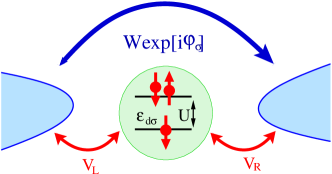
Figure 1: Sketch of the system under consideration. A two-lead Aharonov-Bohm interferometer has a quantum dot embedded in its lower arm. $W$ is the transmission amplitude in the direct path whereas $V_{\alpha}$ ($\alpha=L/R$) are hopping matrix elements between the dot and the leads. The electrons traveling along the ring can acquire a spin-dependent phase $\phi_{\sigma}$. We consider a quantum dot with a single energy level $\varepsilon_{d}$ and charging energy $U$.

II.1 Noninteracting case

We first review the non-interacting case ($U=0$).ver09 We define the quantum-dot retarded Green function for electrons with spin $\sigma$,

$${\cal{G}}_{d\sigma}^{r}(\omega)=\int_{-\infty}^{\infty}dt\,e^{i\omega t}\langle\langle d_{\sigma}(t),d_{\sigma}^{\dagger}(0)\rangle\rangle^{r}\,,$$ (3)

where $\langle\langle d_{\sigma}(t),d_{\sigma}^{\dagger}(0)\rangle\rangle^{r}=-i\Theta(t)\langle[d_{\sigma}(t),d_{\sigma}^{\dagger}(0)]_{+}\rangle$. The Green function can be calculated exactly as,

$${\cal{G}}_{d\sigma}(\omega)=\frac{1}{\omega-\varepsilon_{d\sigma}-\Sigma_{0\sigma}}\,,$$ (4)

where the zeroth-order (i.e., noninteracting) self-energy reads,

$$\Sigma_{0\sigma}=\frac{{\cal{A}}(V_{L}^{2}+V_{R}^{2}+2V_{L}V_{R}W\cos(\phi_{\sigma}){\cal{A}})}{1-W^{2}{\cal{A}}^{2}}\,,$$ (5)

with

$${\cal{A}}(z\to\omega+i0^{+})\equiv\sum_{k}\frac{1}{z-\varepsilon_{k\sigma}}\,.$$ (6)

In the wide-band limit, the self-energy can be written as

$$\Sigma_{0\sigma}=-\widetilde{\Gamma}\left(i+\sqrt{\alpha\xi}\cos(\phi_{\sigma})\right)\,,$$ (7)

with $\rho_{0}=\rho(E_{F})$, $\xi=\pi^{2}\rho_{0}^{2}W^{2}$, $\alpha=4V_{L}^{2}V_{R}^{2}/(V_{L}^{2}+V_{R}^{2})^{2}$, and $\widetilde{\Gamma}\equiv\Gamma/(1+\xi)=\pi\rho_{0}(V_{L}^{2}+V_{R}^{2})/(1+\xi)$. From Eq. (7), we note that the real part of the self-energy, $\operatorname{Re}\left[\Sigma_{0\sigma}\right]$, is spin-dependent because of the factor $\cos\phi_{\sigma}$. In turn, this implies that there is an effective Zeeman field,

$$g\mu_{B}B_{\rm eff}=\widetilde{\Gamma}\sqrt{\alpha\xi}\sin\phi_{AB}\sin\phi_{\rm SO}\,,$$ (8)

acting on the dot levels due to the combined effect of the local Rashba interaction and the magnetic flux. This effect appears because the phase acquired by an electron with a given spin orientation is $\phi_{AB}+\phi_{SO}$ whereas the opposite orientation acquires $\phi_{AB}-\phi_{SO}$. In fact, if either $\phi_{AB}$ or $\phi_{\rm SO}$ vanish, we have $B_{\rm eff}=0$. Then, quite generally, $B_{\rm eff}$ can lead to net spin polarizations in the transmitted current.sun05 ; hea08

Trivially, such effective field can be canceled by an externally applied field $B_{\rm ext}$ such that $B_{\rm ext}=-B_{\rm eff}\equiv B_{c}$ which compensates the splitting. We see that the compensation field $B_{c}$ is a periodic function of $\phi_{AB}$ and $\phi_{\rm SO}$. Our next goal is to include interactions.

II.2 Mean-field approximation

In the simplest approach that includes interaction,anderson61 one replaces $\varepsilon_{d\sigma}$ with $E_{d\sigma}=\varepsilon_{d\sigma}+U\langle n_{\bar{\sigma}}\rangle$ in Eq. (4), where the mean dot occupation at equilibrium reads,

$$\langle n_{\sigma}\rangle=-\frac{1}{\pi}\int_{-\infty}^{\infty}d\omega\,f(\omega)\,{\rm Im}\,{\cal{G}}_{d\sigma}^{r}(\omega)\,$$ (9)

with $f(\omega)$ the Fermi distribution function. The problem, thus, must be self-consistently solved since the right-hand side of Eq. (9) depends on $\langle n_{\sigma}\rangle$. This Hartree approach is known to generate local magnetic moments, even in the presence of spin-orbit interactions.cri09 To avoid this, we will here focus on the nonmagnetic phase.

We extend the method of Ref. hor, to account for both the AB and the spin-orbit phases. Then, we obtain for the special point $\varepsilon_{d}=-U/2$ the self-consistent equation,

$$E_{d\sigma}=-\sigma\frac{U}{\pi}\tan^{-1}\left(\frac{Um}{2\widetilde{\Gamma}}\right)-\widetilde{\Gamma}\sqrt{\alpha\xi}\cos(\phi_{\sigma})\,,$$ (10)

Here, $m=\langle n_{\uparrow}\rangle-\langle n_{\downarrow}\rangle$ is the dot magnetization. The compensating field is calculated from the condition $m=0$, which is satisfied by

$$g\mu_{B}B_{c}=-\widetilde{\Gamma}\sqrt{\alpha\xi}\sin\phi_{AB}\sin\phi_{\rm SO}\,.$$ (11)

We note this value coincides with the noninteracting result obtained above. Therefore, to find corrections to the noninteracting case we must go beyond the mean-field approach and include strong correlations. We first analyze the problem numerically and then later we perform a scaling study that demonstrates that there are indeed corrections due to interactions but, strikingly, the periodicity of $B_{c}$ is preserved.

III Numerical Renormalization Group Calculation

We now present a numerical renormalization group (NRG) analysis of our system. Employing the standard NRG recipe Kri80 and an even/odd parity basis,

$$f_{ne\sigma} =\frac{1}{\sqrt{2}}\left(e^{-i\phi_{\sigma}/2}f_{nL\sigma}+e^{+i\phi_{\sigma}/2}f_{nR\sigma}\right)\,,$$ (12a)

$$f_{no\sigma} =\frac{1}{\sqrt{2}}\left(ie^{-i\phi_{\sigma}/2}f_{nL\sigma}-ie^{+i\phi_{\sigma}/2}f_{nR\sigma}\right)\,,$$ (12b)

we first map the continuous conduction bands onto the corresponding tight-binding model. Here, a symmetric coupling is taken, i.e., $V_{L}=V_{R}\equiv V_{1}$. The resulting Hamiltonian can be then written as

$${\cal{H}}=\sum_{\sigma}\sqrt{\frac{2\Gamma}{\pi}}\left(\cos(\phi_{\sigma}/2)d_{\sigma}^{\dagger}f_{0e\sigma}+\sin(\phi_{\sigma}/2)d_{\sigma}^{\dagger}f_{0o\sigma}+h.c.\right)\\ +\frac{1+\Lambda^{-1}}{2}\sum_{\alpha=e/o}\sum_{n=0}^{\infty}\sum_{\sigma}\Lambda^{-n/2}\zeta_{n}\left(f_{n\alpha\sigma}^{\dagger}f_{n+1\alpha\sigma}+h.c.\right)\\ +\frac{2}{\pi}\sqrt{\xi}\sum_{\sigma}\left(f_{0e\sigma}^{\dagger}f_{0e\sigma}-f_{0o\sigma}^{\dagger}f_{0o\sigma}\right)+{\cal{H}}_{D}\,.$$ (13)

Here, we assume a constant conduction band with a half-width $D$. Note that the couplings between lead and dot are now spin-dependent. To solve the Hamiltonian, we define a sequence of Hamiltonians $\bar{{\cal{H}}}_{N}$ as follows:

$$\bar{{\cal{H}}}_{N}=\Lambda^{(N-1)/2}\left\{{\cal{H}}_{D}\right.\\ +\sum_{\sigma}\sqrt{\frac{2\Gamma}{\pi}}\left(\cos(\phi_{\sigma}/2)d_{\sigma}^{\dagger}f_{0e\sigma}+\sin(\phi_{\sigma}/2)d_{\sigma}^{\dagger}f_{0o\sigma}+h.c.\right)\\ +\frac{1+\Lambda^{-1}}{2}\sum_{\alpha=e/o}\sum_{n=0}^{N-1}\sum_{\sigma}\Lambda^{-n/2}\zeta_{n}\left(f_{n\alpha\sigma}^{\dagger}f_{n+1\alpha\sigma}+h.c.\right)\\ \left.+\frac{2}{\pi}\sqrt{\xi}\sum_{\sigma}\left(f_{0e\sigma}^{\dagger}f_{0e\sigma}-f_{0o\sigma}^{\dagger}f_{0o\sigma}\right)\right\}\,,$$ (14)

that results in the recursion relation below

$$\widetilde{{\cal{H}}}_{N+1}=\sqrt{\Lambda}\widetilde{{\cal{H}}}_{N}+\sum_{\alpha=e/o}\sum_{\sigma}\zeta_{n}\left(f_{N\alpha\sigma}^{\dagger}f_{N+1\alpha\sigma}+h.c.\right)\,,$$ (15)

with

$$\widetilde{{\cal{H}}}_{N}=\frac{2}{1+\Lambda^{-1}}\bar{{\cal{H}}}_{N}\,.$$ (16)

Using this recursion relation, we iteratively diagonalize the NRG Hamiltonian and keep only the lowest eigenvalues in each step. In doing so, however, we have to be careful because the original Wilson’s NRG approachwilson fails in the presence of a magnetic field. This failure results from the fact that at the initial stages the Wilson’s approach does not yet know about the tiny perturbation breaking the spin symmetry and thus yields an incorrect ground state. Here, we thus employ the so-called density-matrix (DM) NRG approach developed by Hofstetter.Hof00 Although there exist more sophisticated methods in the literature,Wei07 we believe the DM-NRG is enough for our purposes.

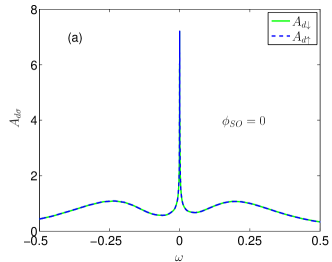
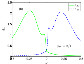
Figure 2: Spectral weights. Parameters are $D=1$, $\varepsilon_{d}=-0.25$, $U=0.5$, $V_{1}=0.1414$, $\xi=1$, $\phi_{AB}=\pi/4$. The spin-orbit coupling strengths are (a) $\phi_{SO}=0$ and (b) $\pi/4$.

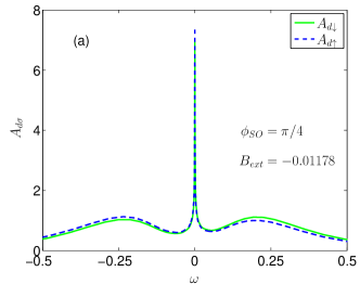
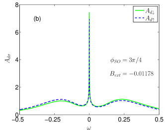
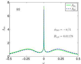
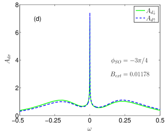
Figure 3: Compensation effect. The spin-orbit strengths are (a) $\phi_{SO}=\pi/4$, (b) $\phi_{SO}=3\pi/4$, and (c) $\phi_{SO}=-\pi/4$, and (d) $\phi_{SO}=-3\pi/4$. Parameters are $D=1$, $\varepsilon_{d}=-0.25$, $U=0.5$, $V_{1}=0.1414$, $\xi=1$, and $\phi_{AB}=\pi/4$.

In Fig. 2, we show for both spin up and spin down the spectral weights of the dot as a function of the Rashba spin-orbit interaction $\phi_{SO}$ for $\phi_{AB}=\pi/4$. Without spin-orbit interactions [Fig. 2(a)], both spectral weights coincide and do not split. However, for $\phi_{SO}=\pi/4$ [Fig. 2(b)] the weights split and the Kondo resonances near the Fermi level become suppressed.ver09 Moreover, the spectral weights move to the particle (hole) sector for spin up (down). Such a shift results from the polarization of the dot occupation.

The split Kondo peaks can be compensated by applying an external magnetic field. Figure 3 shows the recovery of the Kondo resonance at the Fermi level for various values of $\phi_{SO}$. We observe that the compensating fields for $\phi_{SO}=\pi/4(3\pi/4)$ and $-\pi/4(-3\pi/4)$ have opposite signs. Therefore, the effective field is invariant under simultaneous reversal of both the AB flux and the Rashba interaction. This fact is understood in the noninteracting case from Eq. (8). Hence, it is crucial to investigate in detail the precise form of the compensating field in the presence of interactions. This goal can be accomplished only via a scaling analysis, which we perform in the next section.

IV Scaling Analysis

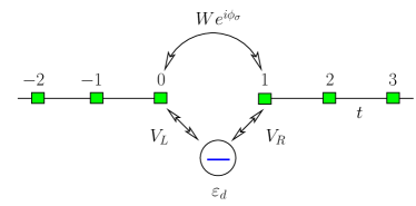
Figure 4: AB ring with spin-orbit interaction of the Rashba type and coupled to semi-infinite discrete leads.

IV.1 Tight-Binding Model and Lead Polarization

The scaling analysis is greatly simplified if we consider a tight-binding model of the system. We discretize the leads and consider the system shown in Fig. 4. The model Hamiltonian is given by

$${\cal{H}}={\cal{H}}_{D}+{\cal{H}}_{C}+{\cal{H}}_{T}\,,$$ (17)

where

$${\cal{H}}_{D} =\sum_{\sigma}\varepsilon_{d\sigma}d_{\sigma}^{\dagger}d_{\sigma}+Un_{d\uparrow}n_{d\downarrow}\,,$$ (18a)

$${\cal{H}}_{C} =\sum_{n\neq 0}\sum_{\sigma}\left(-tc_{n+1\sigma}^{\dagger}c_{n\sigma}+h.c.\right)$$

$$+\sum_{\sigma}\left(We^{i\phi_{\sigma}}c_{0,\sigma}^{\dagger}c_{1,\sigma}+h.c.\right)\,,$$ (18b)

$${\cal{H}}_{T} =\sum_{\sigma}\left(V_{L}d_{\sigma}^{\dagger}c_{0,\sigma}+V_{R}d_{\sigma}^{\dagger}c_{1,\sigma}+h.c.\right)\,.$$ (18c)

The only difference with our starting Hamiltonian Eq. (1) is the distinct representation of the leads but this does not change the underlying physics.

The Hamiltonian Eq. (17) has been considered in Ref. yos08, for the case without spin-orbit interactions. It is shown that an AB ring with an embedded quantum dot threaded by $\phi_{AB}$ can be mapped onto an equivalent Anderson model in which the density of states in the transformed lead has a term proportional to $\varepsilon_{k\sigma}\cos(\phi_{AB})$ in addition to a constant.yos08 Following their approach, we first diagonalize the lead Hamiltonian ${\cal{H}}_{C}$. Using this diagonalized basis and neglecting the decoupled mode, we find that Eq. (17) becomes,

$${\cal{H}}={\cal{H}}_{D}+\sum_{k,\sigma}\varepsilon_{k\sigma}c_{sk\sigma}^{\dagger}c_{sk\sigma}+\sum_{\sigma}V\left[d_{\sigma}^{\dagger}c_{sk\sigma}+h.c.\right]\,,$$ (19)

where the effective density of states in the lead reads

$$\rho_{\sigma}(\varepsilon_{k\sigma})=\widetilde{\rho}_{0}\left(1+\sqrt{\alpha{\cal{T}}_{b}}\cos(\phi_{\sigma})\frac{\varepsilon_{k\sigma}}{D_{0}}\right)\,,$$ (20)

with $V=\sqrt{V_{L}^{2}+V_{R}^{2}}$, $x=(V_{2}/t)^{2}$ (which amounts to $\xi$ in the continuum model of leads, see Sec. II), $\widetilde{\rho}_{0}=1/\pi t(1+x)$, $\alpha=4V_{L}^{2}V_{R}^{2}/(V_{L}^{2}+V_{R}^{2})^{2}$, ${\cal{T}}_{b}=4x/(1+x)^{2}$, and $D_{0}=2t$. Remarkably, from Eq. (20) we observe that the density of states for the reduced lead becomes spin-dependent. Therefore, we expect a spin-dependent coupling between the lead and the dot which will give rise to an effective magnetic field in the dot. This situation is also seen in simple models of ferromagnetic leads attached to Kondo impurities,martinek ; choi ; krawiec but the difference is that while in the latter case the term yielding a spin polarization is constant in energy,martinek ; choi ; krawiec in our case the density of states contains a term linear in $\varepsilon_{k\sigma}$.

To gain further insight into the spin polarized tunnel coupling arisen from Eq. (20), it is sufficient to consider the spin-dependent occupation of the reduced lead at zero temperature,

$$n_{\sigma}=\int_{-D_{0}}^{0}d\varepsilon~{}\rho_{\sigma}(\varepsilon)\,.$$ (21)

Defining the effective spin polarization as

$$P=\frac{n_{\uparrow}-n_{\downarrow}}{n_{\uparrow}+n_{\downarrow}}\,,$$ (22)

we insert Eq. (20) in Eq. (21) and obtain,

$$P=\frac{\sqrt{\alpha{\cal{T}}_{b}}\sin(\phi_{AB})\sin(\phi_{SO})}{2-\sqrt{\alpha{\cal{T}}_{b}}\cos(\phi_{AB})\cos(\phi_{SO})}\,.$$ (23)

We observe that the effective lead polarization $P$ is zero for $\phi_{AB}=n\pi$ or $\phi_{SO}=n\pi$ with $n$ integer and depends on the coupling asymmetry $\alpha$ and the background transmission ${\cal{T}}_{b}$. Moreover, it is worth noting that the fully polarized case ($|P|=1$) can never be achieved since $|P_{\rm max}|=\sqrt{\alpha T_{b}}/2\leq 0.5$.

We now calculate the compensating field in the tight-binding representation with $U=0$. As we know from Sec. II, the effective field arises from the real part of the tunneling self-energy which now reads,

$$\operatorname{Re}\Sigma_{0\sigma}=V^{2}\int^{\prime}d\varepsilon_{k\sigma}\,\frac{\rho(\varepsilon_{k\sigma})}{\omega-\varepsilon_{k\sigma}}\,,$$ (24)

where the prime at the integral means the Cauchy’s principal value. The compensating field occurs at external fields such that $\varepsilon_{d\uparrow}-\varepsilon_{d\downarrow}+\operatorname{Re}(\Sigma_{0\uparrow}-\Sigma_{0\downarrow})=0$ Using Eqs. (20) and (24), we find

$$g\mu_{B}B_{\rm c}=-\widetilde{\Gamma}_{t}\sqrt{\alpha{\cal{T}}_{b}}\sin\phi_{AB}\sin\phi_{\rm SO}\,,$$ (25)

with $\widetilde{\Gamma}_{t}=2\widetilde{\rho}_{0}V^{2}$. This results agrees with the compensating field obtained in the continuum model of Sec. II, see Eq. (8), up to a factor $1/(1+x)$ (or $1/(1+\xi)$). Although the prefactors are different, the functional dependence is the same.

IV.2 Compensating Field

To calculate the effective field for $U\neq 0$, we consider the case when the dot levels lie within the conduction band. Then, scattering processes on a scale $D$ can involve real charge fluctuations of the dot. Taking into account this effect and employing second-order perturbation theory in $V$, we continuously reduce the bandwidth $D$ by a positive infinitesimal $\delta D$. As a consequence, the dot energy levels in the dot are renormalizedHal78 as

$$\varepsilon_{0}^{\prime} =\varepsilon_{0}-\sum_{\sigma}\frac{\rho_{\sigma}(-D)\delta DV^{2}}{\varepsilon_{d\sigma}+D}\,,$$ (26a)

$$\varepsilon_{1\sigma}^{\prime} =\varepsilon_{1\sigma}-\delta DV^{2}\left[\frac{\rho_{\bar{\sigma}}(-D)}{\varepsilon_{d\bar{\sigma}}+U+D}+\frac{\rho_{\sigma}(+D)}{D-\varepsilon_{d\sigma}}\right]\,,$$ (26b)

$$\varepsilon_{2}^{\prime} =\varepsilon_{2}-\sum_{\sigma}\frac{\rho_{\sigma}(+D)\delta DV^{2}}{D-\varepsilon_{d\sigma}-U}\,,$$ (26c)

where $\varepsilon_{0}$ denotes the energy of the empty state, $\varepsilon_{1\sigma}$ the energy of a singly occupied state with spin $\sigma$, and $\varepsilon_{2}$ the energy of the doubly occupied state. Since $\varepsilon_{d\sigma}=\varepsilon_{1\sigma}-\varepsilon_{0}$ by definition, for $U\to\infty$ Eqs. (26) yield the scaling equation for the single-particle energy,

$$\frac{d\varepsilon_{d\sigma}}{d\ln D}=-\frac{\widetilde{\Gamma}_{t}}{2}\left[1-\sqrt{\alpha{\cal{T}}_{b}}\left(2\cos(\phi_{\sigma})+\cos(\phi_{\bar{\sigma}})\right)\frac{D}{D_{0}}\right]\,.$$ (27)

By integrating out the band from $D_{0}$ to $D$, we then obtain the renormalized energy level

$$\widetilde{\varepsilon}_{d\sigma}=\varepsilon_{d\sigma}\\ +\frac{\widetilde{\Gamma}_{t}}{2}\left[\ln\frac{D_{0}}{D}-\sqrt{\alpha{\cal{T}}_{b}}\left(2\cos(\phi_{\sigma})+\cos(\phi_{\bar{\sigma}})\right)\left(1-\frac{D}{D_{0}}\right)\right]\,.$$ (28)

From Eq. (28), we find that the total level splitting $\Delta_{Z}\equiv\widetilde{\varepsilon}_{d\uparrow}-\widetilde{\varepsilon}_{d\downarrow}$ is given by

$$\Delta_{Z}=(\varepsilon_{d\uparrow}-\varepsilon_{d\downarrow})+\widetilde{\Gamma}_{t}\sqrt{\alpha{\cal{T}}_{b}}\sin(\phi_{AB})\sin(\phi_{SO})\left(1-\frac{D}{D_{0}}\right)\,.$$ (29)

from which the effective magnetic field results,

$$g\mu_{B}B_{\rm eff}=\frac{\widetilde{\Gamma}_{t}}{2}\sqrt{\alpha{\cal{T}}_{b}}\sin(\phi_{AB})\sin(\phi_{SO})\left(1-\frac{D}{D_{0}}\right)\,.$$ (30)

Since the scaling terminates at $D=\widetilde{D}$ roughly given by $\widetilde{D}\approx|\widetilde{\varepsilon}_{d}|$, using Eq. (29) the compensating field $B_{c}=-B_{\rm eff}$ is given by

$$g\mu_{B}B_{c}=-\frac{\widetilde{\Gamma}_{t}}{2}\sqrt{\alpha{\cal{T}}_{b}}\sin(\phi_{AB})\sin(\phi_{SO})\left(1+\frac{\widetilde{\varepsilon}_{d}}{D_{0}}\right)\,,$$ (31)

where $\widetilde{\varepsilon}_{d}$ can be found from,

$$\widetilde{\varepsilon}_{d}=\varepsilon_{d}+\frac{\widetilde{\Gamma}_{t}}{2}\ln\frac{D_{0}}{|\widetilde{\varepsilon}_{d}|}-\frac{3\widetilde{\Gamma}_{t}}{2}\sqrt{\alpha{\cal{T}}_{b}}\cos(\phi_{AB})\cos(\phi_{SO})\,.$$ (32)

In the case $|\widetilde{\varepsilon}_{d}|\ll D_{0}$, Eq. (31) predicts that the effective field is half the value for the noninteracting case. As a consequence, strong interactions reduce the external field needed to compensate $B_{\rm eff}$ [see Eq. (25)]. Notably, the functional dependence of $B_{c}$ on $\phi_{AB}$ and $\phi_{SO}$ remains the same.

On the other hand, for the special point $2\varepsilon_{d}+U=0$, the effective level evolves as,

$$\frac{d\varepsilon_{d\sigma}}{d\ln D}=\widetilde{\Gamma}_{t}\sqrt{\alpha{\cal{T}}_{b}}\cos(\phi_{\sigma})\frac{D}{D_{0}}\,,$$ (33)

so that for the compensating field we have,

$$g\mu_{B}B_{c}\approx-\widetilde{\Gamma}_{t}\sqrt{\alpha{\cal{T}}_{b}}\sin(\phi_{AB})\sin(\phi_{SO})\,.$$ (34)

In this case, at $B=B_{c}$ the renormalized energy level reads

$$\widetilde{\varepsilon}_{d}=\varepsilon_{d}-\widetilde{\Gamma}_{t}\sqrt{\alpha{\cal{T}}_{b}}\cos(\phi_{AB})\cos(\phi_{SO})\,.$$ (35)

Equation (34) agrees, except for the prefactor, with the mean-field result obtained earlier, see Eq. (11).

IV.3 Kondo Temperature

The charge fluctuation is quenched at $D<\widetilde{D}$ and only spin fluctuations thus plays a role at lower energies. In order to describe these fluctuations, we perform a Schrieffer-Wolff transformation and obtain the Kondo Hamiltonian given by,

$${\cal{H}}_{K}=\sum_{k,k^{\prime}}\left[J_{+}S_{+}c_{sk^{\prime}\downarrow}^{\dagger}c_{sk\uparrow}+J_{-}S_{-}c_{sk^{\prime}\uparrow}^{\dagger}c_{sk\downarrow}\right.\\ \left.+J_{z\uparrow}S_{z}c_{sk^{\prime}\uparrow}^{\dagger}c_{sk\uparrow}-J_{z\downarrow}S_{z}c_{sk^{\prime}\downarrow}^{\dagger}c_{sk\downarrow}\right]+K\sum_{k,k^{\prime}}\sum_{\sigma}c_{sk^{\prime}\sigma}^{\dagger}c_{sk\sigma}\,,$$ (36)

where

$$J_{\pm,z\sigma} =\frac{V^{2}}{|\widetilde{\varepsilon}_{d}|}+\frac{V^{2}}{U-|\widetilde{\varepsilon}_{d}|}\,,$$ (37a)

$$K =\frac{1}{2}\left(\frac{V^{2}}{|\widetilde{\varepsilon}_{d}|}-\frac{V^{2}}{U-|\widetilde{\varepsilon}_{d}|}\right)\,,$$ (37b)

with renormalized single-particle energy $\widetilde{\varepsilon}_{d}$ and bandwidth $\widetilde{D}$.

Using Poor Man’s scaling,anderson70 the scaling equations for the coupling constants can be then written as

$$\frac{dJ_{z\sigma}}{d\ln D} =-2\widetilde{\rho}_{0}J_{\pm}^{2}\,,$$ (38a)

$$\frac{dJ_{\pm}}{d\ln D} =-\widetilde{\rho}_{0}J_{\pm}\left(J_{z\uparrow}+J_{z\downarrow}\right)\,,$$ (38b)

where we have kept only up to zeroth-order terms in $D/D_{0}$. Since Eqs. (38) break down at $T_{K}$, we obtain

$$k_{B}T_{K}\approx\widetilde{D}\exp\left[-\frac{1}{2\widetilde{\rho}_{0}J}\right]\,.$$ (39)

Here, we assume that the spin splitting has been completely compensated by an external magnetic field, thus employing the renormalized single-particle energy at the compensating field given by Eq. (32). For $U\to\infty$, the Kondo temperature can then be expressed as a function of $\phi_{AB}$ and $\phi_{SO}$:

$$k_{B}T_{K}\approx T_{K}\left(\pi/2\right)\exp\left[-\frac{3}{2}\sqrt{\alpha{\cal{T}}_{b}}\cos(\phi_{AB})\cos(\phi_{SO})\right]\,,$$ (40)

where $T_{K}(\pi/2)$ denotes the Kondo temperature at $\phi_{AB}=\pi/2$ and $\phi_{SO}=\pi/2$. Note that the Kondo temperature is also a sinusoidal function of $\phi_{AB}$ and $\phi_{SO}$. On the other hand, for the case $\varepsilon_{d}=-U/2$ we have

$$k_{B}T_{K}\approx T_{K}(\pi/2)\exp\left[-\frac{\widetilde{\Gamma}_{t}}{2\varepsilon_{d}}\left(\sqrt{\alpha{\cal{T}}_{b}}\cos(\phi_{AB})\cos(\phi_{SO})\right)^{2}\right]\,.$$ (41)

In this case, the flux dependence is much weaker than that of the infinite $U$ case described by Eq. (40).

V Effective Field

The qualitative discussion in Sec. IV.B. demonstrates the existence of an effective field acting on the dot. To gain deeper insight into the properties of the compensating field and investigate its functional dependence on temperature and the gate voltage, we now derive an effective Hamiltonian ${\cal{H}}_{\rm eff}$ using perturbation theory. Physically, the split Kondo peak can be understood in terms of the dot valence instability (virtual charge fluctuation) and spin-dependent density of states. To deal with this instability, we perform a Schrieffer–Wolff-like transformation of the Hamiltonian given by Eq. (19). Then,

$${\cal{H}}_{\rm eff}=\sum_{k,k^{\prime}}\left[\frac{V^{2}}{\varepsilon_{d\uparrow}-\varepsilon_{k^{\prime}\uparrow}}c_{sk\uparrow}c_{sk^{\prime}\uparrow}^{\dagger}-\frac{V^{2}}{\varepsilon_{d\downarrow}-\varepsilon_{k^{\prime}\downarrow}}c_{sk\downarrow}c_{sk^{\prime}\downarrow}^{\dagger}\right.\\ \left.+\frac{V^{2}}{U+\varepsilon_{d\uparrow}-\varepsilon_{k^{\prime}\uparrow}}c_{sk^{\prime}\uparrow}^{\dagger}c_{sk\uparrow}-\frac{V^{2}}{U+\varepsilon_{d\downarrow}-\varepsilon_{k^{\prime}\downarrow}}c_{sk^{\prime}\downarrow}^{\dagger}c_{sk\downarrow}\right]S_{z}\\ +[\cdots]\,,$$ (42)

where $[\cdots]$ includes spin-flip $S_{\pm}$ and potential scatterings. At this point, unlike the usual Schrieffer–Wolff transformation, we employ a mean-field approximation for the lead electrons Kon04

$$\langle c_{sk\sigma}c_{sk^{\prime}\sigma^{\prime}}^{\dagger}\rangle =\left[1-f(\varepsilon_{k\sigma})\right]\delta_{k,k^{\prime}}\delta_{\sigma,\sigma^{\prime}}\,,$$ (43a)

$$\langle c_{sk^{\prime}\sigma^{\prime}}^{\dagger}c_{sk\sigma}\rangle =f(\varepsilon_{k\sigma})\delta_{k,k^{\prime}}\delta_{\sigma,\sigma^{\prime}}\,.$$ (43b)

Then, the spin-flip scattering terms vanish and we obtain,

$${\cal{H}}_{\rm eff}=-V^{2}\int^{\prime}d\omega~{}\left[\rho_{\uparrow}(\omega)\frac{1-f(\omega)}{\omega-\varepsilon_{d\uparrow}}-\rho_{\downarrow}(\omega)\frac{1-f(\omega)}{\omega-\varepsilon_{d\downarrow}}\right.\\ \left.+\rho_{\uparrow}(\omega)\frac{f(\omega)}{\omega-U-\varepsilon_{d\uparrow}}-\rho_{\downarrow}(\omega)\frac{f(\omega)}{\omega-U-\varepsilon_{d\downarrow}}\right]S_{z}\\ +[\text{Potential scattering}]\,.$$ (44)

Since the density of states is spin-dependent in our case, the quantity in the square bracket is nonzero.

The effective Hamiltonian of Eq. (44) can be expressed as

$${\cal{H}}_{\rm eff}=2g\mu_{B}B_{\rm eff}S_{z}=g\mu_{B}B_{\rm eff}\sigma_{z}\,,$$ (45)

from which it follows that

$$g\mu_{B}B_{\rm eff}=-\frac{\widetilde{\Gamma}_{t}}{4}\int^{\prime}d\omega~{}\left\{\right.\\ \left(1+\sqrt{\alpha{\cal{T}}_{b}}\cos(\phi_{\uparrow})\frac{\omega}{D_{0}}\right)\left[\frac{1-f(\omega)}{\omega-\varepsilon_{d\uparrow}}+\frac{f(\omega)}{\omega-U-\varepsilon_{d\uparrow}}\right]\\ \left.-\left(1+\sqrt{\alpha{\cal{T}}_{b}}\cos(\phi_{\downarrow})\frac{\omega}{D_{0}}\right)\left[\frac{1-f(\omega)}{\omega-\varepsilon_{d\downarrow}}+\frac{f(\omega)}{\omega-U-\varepsilon_{d\downarrow}}\right]\right\}\,.$$ (46)

This is the explicit formula of the effective field and is a central result of our work.

For $B_{\rm ext}=0$ ($\varepsilon_{d\uparrow}=\varepsilon_{d\downarrow}$), Eq. (46) can be written as

$$g\mu_{B}B_{\rm eff}=\widetilde{\Gamma}_{t}\sqrt{\alpha{\cal{T}}_{b}}\sin(\phi_{AB})\sin(\phi_{SO})\\ \times\left\{1-\frac{\varepsilon_{d}}{2D_{0}}\widetilde{\Psi}(\varepsilon_{d})+\frac{(U+\varepsilon_{d})}{2D_{0}}\widetilde{\Psi}(U+\varepsilon_{d})\right\}\,,$$ (47)

where

$$\widetilde{\Psi}(\varepsilon)=\ln\frac{2\pi}{\beta D_{0}}+\operatorname{Re}\left[\Psi\left(\frac{1}{2}-i\beta\frac{(\varepsilon-E_{F})}{2\pi}\right)\right]\,.$$ (48)

For low values of $\sqrt{\alpha\mathcal{T}_{b}}$, the effective field is proportional to the lead polarization $P$ [cf. Eq. (23)], $B_{\rm eff}\propto\widetilde{\Gamma}P$, in analogy with a quantum dot coupled to ferromagnetic case.martinek The crucial difference is that in our case, $B_{\rm eff}$ is nonvanishing for noninteracting electrons. Setting $U=0$ in Eq. (47) we recover the expression found above. Therefore, the effective magnetic field is not only generated via exchange interaction between the dot electrons and the leads but it also contains a contribution from the spin-orbit interaction and the magnetic flux when their associated phases are nonzero at the same time.

As shown in the previous sections, the effective field $B_{\rm eff}$ can be compensated by applying an external magnetic field $B_{c}$ such that $B_{c}=-B_{\rm eff}$,note_self

$$g\mu_{B}B_{c}=-\widetilde{\Gamma}_{t}\sqrt{\alpha{\cal{T}}_{b}}\sin(\phi_{AB})\sin(\phi_{SO})\\ \times\left\{1-\frac{\varepsilon_{d}}{2D_{0}}\widetilde{\Psi}(\varepsilon_{d})+\frac{(U+\varepsilon_{d})}{2D_{0}}\widetilde{\Psi}(U+\varepsilon_{d})\right\}\,,$$ (49)

which generalizes our previous expressions [Eq. (31) and Eq. (34)] and is valid for nonzero temperature and interacting electrons. Importantly, the precise dependence on $\phi_{AB}$ and $\phi_{SO}$ remains in terms of periodic functions.

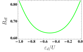
Figure 5: Effective field $B_{\rm eff}$ as a function of $\varepsilon_{d}/U$ with $U/D_{0}=1/2$ at $T=0$. Here, the exchange field $B_{\rm eff}$ has been scaled by $\widetilde{\Gamma}_{t}\sqrt{\alpha{\cal{T}}_{b}}\sin(\phi_{AB})\sin(\phi_{SO})$. Refer to Eq. (47).

In Fig. 5 we show the effective field as a function of the position of the quantum dot level, which can be tuned using a gate voltage. The important result to bear in mind is that $B_{\rm eff}$ is nonzero at the special point $2|\varepsilon_{d}|+U=0$, due to the lack of particle-hole symmetry in our system. This is in stark contrast with the case of ferromagnetic leads. In that case, only the spin fluctuations prevail at the particle-hole symmetric point so that the exchange field coming from charge fluctuations is zero. choi

VI Conclusions

To summarize, we have investigated the splitting that occurs in the density of states of a quantum dot inserted in a mesoscopic interferometer in the presence of spin-orbit interactions and magnetic flux. In the Kondo regime, the resonance at the Fermi energy becomes split at nonzero values of both the Aharonov-Bohm and the Rashba phases. The splitting is due to an effective field whose main properties can be more clearly derived from the instructive mapping to a Hamiltonian that describes a quantum dot coupled to a transformed lead with spin-dependent density of states. As a consequence, the coupling between the dot and the lead depends on the spin orientation and an effective Zeeman splitting emerges.

For interacting electrons, a study of charge fluctuations within a scaling procedure reveals an effective magnetic field that increases with the charging energy. Importantly, the correction becomes of the same order as the noninteracting value for $U\to\infty$.

The splitting can be compensated with an external magnetic field. We have calculated the compensating field for both interacting and noninteracting electrons. In both cases we obtain an expression which shows that the compensating field is a periodic function of the Aharonov-Bohm and the spin-orbit phases. We have also emphasized the breaking of particle-hole symmetry in our system, which implies a nonzero value of the effective field regardless of the applied gate voltage.

References

(1)
A. Yacoby, M. Heiblum, D. Mahalu, and H. Shtrikman,
Phys. Rev. Lett. 74, 4047 (1995).
(2)
A. Levy Yeyati and M. Büttiker,
Phys. Rev. B 52, R14360 (1995).
(3)
G. Hackenbroich and H.A. Weidenmüller,
Phys. Rev. Lett. 76, 110 (1996).
(4)
C. Bruder, R. Fazio and H. Schoeller,
Phys. Rev. Lett. 76, 114 (1996).
(5)
R. Schuster, E. Buks, M. Heiblum, D. Mahalu,
V. Umansky and H. Shtrikman, Nature 385, 417 (1997).
(6)
Y. Ji, M. Heiblum, D. Sprinzak, D. Mahalu, and H. Shtrikman,
Science 290, 779 (2000).
(7)
M. Sigrist, A. Fuhrer, T. Ihn, K. Ensslin, S.E. Ulloa,
W. Wegscheider, and M. Bichler,
Phys. Rev. Lett. 93, 066802 (2004).
(8)
K. Kobayashi, H. Aikawa, S. Katsumoto, and Y. Iye,
Phys. Rev. Lett. 88, 256806 (2002).
(9)
A. C. Hewson, The Kondo Problem to Heavy Fermions (Cambridge University Press, Cambridge, 1993).
(10)
D. Goldhaber-Gordon, H. Shtrkman, D. Mahalu, D. Abusch-Magder, U. Meirav,
M. A. Kastner, Nature 391, 156 (1998); S. M. Cronenwett, T. H. Oosterkamp, and L. P. Kouwenhoven, Science 281, 540 (1998);
J. Schmid, J. Weis, K. Eberl, and K. von Klitzing, Physica B 256, 182 (1998).
(11)
W. Hofstetter, J. König, and H. Schoeller,
Phys. Rev. Lett. 87, 156803 (2001).
(12)
B.R. Bulka and P. Stefański,
Phys. Rev. Lett. 86, 5128 (2001).
(13)
For a recent review, see, e.g, J. Fabian, A. Matos-Abiague, C. Ertler, P. Stano, and I. Zutic,
Acta Physica Slovaca 57, 565 (2007).
(14) E. I. Rashba,
Fiz. Tverd, Tela (Leningrad) 2, 1224 (1960). [Sov. Phys. Solid State 2, 1109 (1960)]
(15)
A. F. Morpurgo, J. P. Heida, T. M. Klapwijk, B. J. van Wees, and G. Borghs,
Phys. Rev. Lett. 80, 1050 (1998).
(16)
J. B. Yau, E. P. De Poortere, and M. Shayegan,
Phys. Rev. Lett. 88, 146801 (2002).
(17)
M. J. Yang, C. H. Yang, and Y. B. Lyanda-Geller,
Europhys. Lett. 66, 826 (2004).
(18)
B. Grbić, R. Leturcq, T. Ihn, K. Ensslin, D. Reuter, and A. D. Wieck,
Phys. Rev. Lett. 99, 176803 (2007).
(19)
Q.F. Sun, J. Wang, and H. Guo, Phys. Rev. B 71, 165310 (2005);
Q.-f.Sung and X.C. Xie, Phys. Rev. B 73, 235301 (2006).
(20)
R. López, D. Sánchez, and Ll. Serra, Phys. Rev. B 76, 035307 (2007).
(21)
M. Crisan, D. Sánchez, R. López, Ll. Serra, and I. Grosu,
Phys. Rev. B 79, 125319 (2009).
(22)
R.J. Heary, J.E. Han, and L. Zhu, Phys. Rev. B 77, 115132 (2008).
(23)
E. Vernek, N. Sandler, and S. E. Ulloa,
Phys. Rev. B 80, 041302(R) (2009).
(24)
J. Martinek, Y. Utsumi, H. Imamura, J. Barnaś, S. Maekawa, J. König, and G. Schön,
Phys. Rev. Lett. 91, 127203 (2003);
J. Martinek, M. Sindel, L. Borda, J. Barnaś, J. König, G. Schön, and J. von Delft,
Phys. Rev. Lett. 91, 247202 (2003).
(25)
R. López and D. Sánchez,
Phys. Rev. Lett. 90, 116602 (2003);
M.-S. Choi, D. Sánchez, and R. López,
Phys. Rev. Lett. 92, 056601 (2004).
(26)
M. Krawiec, J. Phys.: Condens. Matter 19, 346234 (2007).
(27)
We have neglected the Zeeman interaction due to the
applied magnetic flux since in experimentally available
mesoscopic interferometers the applied fields are usually
quite small (of the order of mT).morpurgo ; grbic
(28)
P. W. Anderson, Phys. Rev. 124, 41 (1961).
(29)
B. Horvatić, D. Sokcević, and V. Zlatić,
Phys. Rev. B 36, 675 (1987).
(30)
K. G. Wilson, Rev. Mod. Phys. 47, 773 (1975).
(31)
H. R. Krishna-murthy, J. W. Wilkins, and K. G. Wilson, Phys. Rev. B 21, 1003 (1980).
(32) W. Hofstetter, Phys. Rev. Lett. 85, 1508.
(33) R. Peters, T. Pruschke, and F. B. Anders, Phys. Rev. B 74, 245114 (2006);
A. Weichselbaum and J. von Delft, Phys. Rev. Lett. 99, 076402 (2007).
(34)
R. Yoshii and M. Eto,
J. Phys. Soc. Jap. 77, 123714 (2008).
(35)
F. D. M. Haldane, Phys. Rev. B. 40, 416 (1978).
(36)
P. W. Anderson, Phys. Rev. 3, 2436 (1970).
(37)
J. König, J. Martinek, J. Barnaś, and G. Schön, in CFN Lectures on Functional Nanostructures,
Eds. K. Busch et al., Lecture Notes in Physics 658, Springer, pp. 145-164 (2005).
(38)
We emphasize, however, that
depends on , see the denominators in Eq. (46).
As a consequence, the condition must be solved self-consistently.
Nevertheless, for the problem we consider here we have checked that including
self-consistency merely introduces unimportant corrections to the value
predicted by Eq. (49).