The Dynamic ECME Algorithm

Abstract

The ECME algorithm has proven to be an effective way of accelerating the EM algorithm for many problems. Recognising the limitation of using prefixed acceleration subspaces in ECME, we propose a new Dynamic ECME (DECME) algorithm which allows the acceleration subspaces to be chosen dynamically. Our investigation of the classical Successive Overrelaxation (SOR) method, which can be considered as a special case of DECME, leads to an efficient, simple, stable, and widely applicable DECME implementation, called DECME_v1. The fast convergence of DECME_v1 is established by the theoretical result that, in a small neighbourhood of the maximum likelihood estimate (MLE), DECME_v1 is equivalent to a conjugate direction method. Numerical results show that DECME_v1 and its two variants often converge faster than EM by a factor of one hundred in terms of number of iterations and a factor of thirty in terms of CPU time when EM is very slow.

1 Introduction

After its booming popularity of 30 years since the publication of Dempster et al. (1977), the EM algorithm is still expanding its application scope in various areas. At the same time, to overcome the slow convergence of EM, quite a few extensions of EM have been developed in such a way that they run faster than EM while maintaining its widely recognised simplicity and stability. We refer to Varadhan and Roland (2008) for a recent nice review of various methods for accelerating EM. In the present paper, we start by exploring the convergence of the ECME algorithm (Liu and Rubin, 1994), which has proved to be a simple and effective method to accelerate its parent EM algorithm (see, e.g., Sammel and Ryan, 1996; Kowalski et al., 1997; Pinheiro et al., 2001), to name a few.

ECME is a simple extension of the ECM algorithm (Meng and Rubin, 1993) which itself is an extension of EM. These three algorithms are summarised as follows. Let $Y_{obs}$ be the observed data. Denote by $L(\theta|Y_{obs}),\ \ \theta\in\Theta\subset\mathcal{R}^{p}$, the observed log-likelihood function of $\theta$. The problem is to find the MLE $\hat{\theta}$ that maximises $L(\theta|Y_{obs})$. Let $Y=(Y_{obs},\ Y_{mis})$ represent the complete data with $Y_{obs}$ augmented by the missing data $Y_{mis}$. As an iterative algorithm, the $t$th iteration of EM consists of the E-step, which computes $Q(\theta|Y_{obs},\theta_{t-1})$, the expected complete-data log-likelihood function given the observed data and the current estimate $\theta_{t-1}$ of $\theta$, and the M-step, which finds $\theta=\theta_{t}$ to maximise $Q(\theta|Y_{obs},\theta_{t-1})$.

The ECM algorithm replaces the M-step with a sequence of simpler constrained or conditional maximisation (CM) steps, indexed by $s=1,\cdots,S$, each of which fixes some function of $\theta$, $h_{s}(\theta)$. The ECME algorithm further partitions the $S$ CM-steps into two groups $\mathscr{S}_{Q}$ and $\mathscr{S}_{L}$ with $\mathscr{S}_{Q}\cup\mathscr{S}_{L}=\{1,\cdots,S\}$. While the CM-steps indexed by $s\in\mathscr{S}_{Q}$ (refereed to as the $MQ$-steps) remain the same with ECM, the CM-steps indexed by $s\in\mathscr{S}_{L}$ (refereed to as the $ML$-steps) maximise $L(\theta|Y_{obs})$ in the subspace induced by $h_{s}(\theta)$. A more general framework that includes ECM and ECME as special cases is developed in Meng and van Dyk (1997). However, most of the practical algorithms developed under this umbrella belong to the scope of a simple case, i.e., the parameter constraints are formed by creating a partition, $\mathscr{P}$, of $\theta$ as $(\theta_{1},\ \cdots,\ \theta_{S})$ with associated dimensions $(d_{1},\ \cdots,\ d_{S})$. Mathematically we have $h_{s}(\theta)=(\theta_{1},\ \cdots,\ \theta_{s-1},\ \theta_{s+1},\cdots,\ \theta_{S})$ for $s=1,\cdots,S$.

The advantage of ECME over EM in terms of efficiency depends on the relationship between the slowest converging directions of EM and the acceleration subspaces of ECME, i.e., the subspaces for the $ML$-steps. For example, when the former is effectively embedded within the latter, ECME achieves its superior gain of efficiency over its parent EM. In practise, we usually have no information about the convergence of EM before obtaining the MLE and cannot select the prefixed acceleration subspaces of ECME accordingly. Hence small or minor efficiency gain by ECME is expected in some situations. This is illustrated by the two examples in Section 2 and motivates the idea of dynamically constructing subspaces for applying the $ML$-step. This idea is formulated as the generic DECME algorithm. It includes SOR as a special case. SOR was first developed as an accelerator for a class of iterative solvers of linear systems in 1950’s (Frankel, 1950; Young, 1954). The same idea has been frequently explored in the context of EM (Salakhutdinov and Roweis, 2003; Hesterberg, 2005, among many others although sometimes under different names). However, as shown later, SOR suffers from what is known as the zigzagging problem. Hence it is often inefficient.

Motivated by the zigzagging phenomenon observed on SOR, we propose an efficient DECME implementation, called DECME_v1. It is shown that, under some common assumptions, DECME_v1 is equivalent to a conjugate direction method, which has been proposed in several different contexts, e.g., solving linear systems (Concus et al., 1976) and nonorthogonal analysis of variance (Golub and Nash, 1982). Jamshidian and Jennrich (1993) propose to use the conjugate direction method to accelerate EM. They call the resulting method AEM and demonstrate its dramatically improved efficiency. However, AEM is not as popular as one would expect it to be. This is perhaps due to its demands for extra efforts for coding the gradient vector of $L(\theta|Y_{obs})$, which is problem specific and can be expensive to evaluate.

Compared to AEM, DECME_v1 is simpler to implement because it does not require computing the gradient of $L(\theta|Y_{obs})$. It does require function evaluations, which are typically coded with EM implementation for debugging and monitoring convergence. As SOR, the only extra requirement for implementing DECME_v1 is a simple line search scheme. Such a line search scheme can be used for almost all EM algorithms for different models. To reduce the number of function evaluations, two variants of DECME_v1, called DECME_v2 and DECME_v3, are also considered. Numerical results show that all the three new DECME implementations obtain dramatic efficiency improvement over EM, ECME, and SOR in terms of both number of iterations and CPU time.

The remaining of the paper is arranged as follows. Section 2 provides a pair of motivating ECME examples. Section 3 defines the generic DECME algorithm, discusses the convergence of SOR, and proposes the three efficient novel implementations of DECME. Section 4 presents several numerical examples to compare the performance of different methods. Section 5 concludes with a few remarks.

2 Two Motivating ECME Examples

Following Dempster et al. (1977), in a small neighbourhood of $\hat{\theta}$, we have approximately

$$\hat{\theta}-\theta_{t}=DM^{EM}(\hat{\theta}-\theta_{t-1}),$$ (1)

where the $p\times p$ matrix $DM^{EM}$ is known as the missing information fraction and determines the convergence rate of EM. More specifically, each eigenvalue of $DM^{EM}$ determines the convergence rate of EM along the direction of its corresponding eigenvector (see review in Appendix B).

It is shown in Liu and Rubin (1994) that ECME also has a linear convergence rate determined by the $p\times p$ matrix $DM^{ECME}$ that plays the same role for ECME as $DM^{EM}$ does for EM. Obviously, ECME will be faster than EM if the largest eigenvalue of $DM^{ECME}$ is smaller than that of $DM^{EM}$. With the following two examples we illustrate that it is the choice of the acceleration subspaces by ECME that determines the relative magnitude of the dominating eigenvalues of $DM^{EM}$ and $DM^{ECME}$, and hence the relative efficiency of EM and ECME. All the numerical examples in this paper are implemented in R (R Development Core Team, 2008).

2.1 A Linear Mixed-effects Model Example

Consider the rat population growth data in Gelfand et al. (1990, Tables 3, 4). Sixty young rats were assigned to a control group and a treatment group with $n=30$ rats in each. The weight of each rat was measured at ages $x=8,\ 15,\ 22,\ 29$ and $36$ days. We denote by $y_{i}^{g}$ the weights of the $i$th rat in group $g$ with $g=c$ for the control group and $g=t$ for the treatment group. The following linear mixed-effects model (Laird and Ware, 1982) is considered in Liu (1998):

$$y_{i}^{g}|\theta\sim N(X\beta_{g}+Xb_{i}^{g},\ \sigma_{g}^{2}I_{5}),\ \ b_{i}^{g}\sim N(0,\Psi),$$ (2)

for $i=1,\cdots,n$ and $g=c$ and $t$, where $X$ is the $5\times 2$ design matrix with a vector of ones as its first column and the vector of the five age-points as its second column, $\beta_{g}=(\beta_{g,1},\beta_{g,2})^{\prime}$ contains the fixed effects, $b_{i}^{g}=(b_{i,1}^{(g)},b_{i,2}^{(g)})^{\prime}$ contains the random effects, $\Psi>0$ is the $2\times 2$ covariance matrix of the random effects, and $\theta$ is the vector of the parameters, that is, $\theta=(\beta_{c,1},\beta_{c,2},\beta_{t,1},\beta_{t,2},\Psi_{1,1},\Psi_{1,2},\Psi_{2,2},\sigma_{c}^{2},\sigma_{t}^{2})^{\prime}$. Let $\beta=(\beta_{c,1},\beta_{c,2},\beta_{t,1},\beta_{t,2})^{\prime}$ and $\sigma^{2}=(\sigma_{c}^{2},\sigma_{t}^{2})^{\prime}$. The starting point for running EM and ECME is chosen to be $\beta=(0,0,0,0)^{\prime},\ \sigma^{2}=(1,1)^{\prime}$, and $\Psi=I_{2}$. The stopping criterion used here is given in Section 4.1.

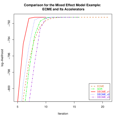
Figure 2: Comparison for the Linear Mixed-effects Model Example in Section 2.1 and Section 4.2. Displayed are increases in $L(\theta|Y_{obs})$, cont’d

For this example, ECME converges dramatically faster than EM, as shown in Figures 1 and 2 and Tables 5 and 6. Specifically, EM takes $5,968$ iterations and $518.9$ seconds to converge. With the same setting, ECME (version 1 in Liu and Rubin (1994) with $\theta_{\mathscr{P}_{Q}}=(\Psi_{11},\Psi_{12},\Psi_{22},\sigma^{2^{\prime}})^{\prime}$ and $\theta_{\mathscr{P}_{L}}=\beta$) uses only 20 iterations and $1.8$ seconds. The gain of ECME over EM is explained clearly by the relation between the slow converging directions of EM and the partition of the parameter space for ECME. From Table 1, the two largest eigenvalues of $DM^{EM}$ are $0.9860$ and $0.9746$, which are close to 1 and make EM converge very slow. From Table 2, it is clear that the first four “worst” directions of EM fall entirely in the subspace determined by the fixed effect $\beta$. Since $\theta_{\mathscr{S}_{L}}=\beta$ for ECME, the slow convergence of EM induced by the four slowest directions is diminished by implementing the $ML$-step along the subspace of $\beta$. This is clear from the row ECME in Table 1, where we see the four largest eigenvalues of $DM^{EM}$ become 0 in $DM^{ECME}$ while the five small eigenvalues of $DM^{EM}$ remain the same for $DM^{ECME}$.

2.2 A Factor Analysis Model Example

Consider the confirmatory factor analysis model example in Jöreskog (1969), Rubin and Thayer (1982), and Liu and Rubin (1998). The data is provided in Liu and Rubin (1998) and the model is as follows. Let $Y$ be the observable nine-dimensional variable on an unobservable variable $Z$ consisting of four factors. For $n$ independent observations of $Y$, we have

$$Y_{i}|(Z_{i},\beta,\sigma^{2})\sim N(Z_{i}\beta,\mathsf{diag}(\sigma_{1}^{2},\cdots,\sigma_{9}^{2}))$$ (3)

where $\beta$ is the $4\times 9$ factor-loading matrix, $\sigma^{2}=(\sigma_{1}^{2},\cdots,\sigma_{9}^{2})^{\prime}$ is called the vector of uniquenesses, and given $(\beta,\sigma^{2})$, $Z_{1},\cdots,Z_{n}$ are independently and identically distributed with $Z_{i}\sim N(0,I_{4}),i=1,\cdots,n$. In the model, there are zero factor loadings on both factor $4$ for variables 1-4 and on factor 3 for variables 5-9. Let $\beta_{j\cdot},\ j=1,\cdots,4$ be the four rows of $\beta$, then the vector of the $36$ free parameters is $\theta=(\beta_{1\cdot},\beta_{2\cdot},\beta_{3,1-4},\beta_{4,5-9},\sigma^{2})^{\prime}$. Liu and Rubin (1998) provided detailed comparison between EM and ECME. Figure 1 of Liu and Rubin (1998) shows that the gain of ECME over EM is impressive, but not as significant as ECME for the previous linear mixed-effects model example in Section 2.1.

The slow convergence of EM for this example is easy to explain from Table 3 which shows that $DM^{EM}$ has multiple eigenvalues close to 1. From Table 4, the eigenvector corresponding to the dominant eigenvalue of $DM^{EM}$ falls entirely in the subspace spanned by $\beta_{1}$ and $\beta_{2}$. This clearly adds difficulty to the ECME version suggested by Liu and Rubin (1998) where $\theta_{\mathscr{S}_{Q}}=(\beta_{1\cdot},\beta_{2\cdot},\beta_{3,1-4},\beta_{4,5-9})^{\prime}$ and $\theta_{\mathscr{S}_{L}}=\sigma^{2}$. For this version of ECME, the eigenvalues of $DM^{ECME}$ are given in row ECME-1 of Table 3, where we see that the dominant eigenvalue of $DM^{EM}$ remains unchanged for $DM^{ECME}$. To eliminate the effect of the slowest direction of EM, we can try another version of ECME by letting $\theta_{\mathscr{S}_{Q}}=\sigma^{2}$ and $\theta_{\mathscr{S}_{L}}=(\beta_{1\cdot},\beta_{2\cdot},\beta_{3,1-4},\beta_{4,5-9})^{\prime}$. The eigenvalues of $DM^{ECME}$ for this version are given in row ECME-2 of Table 3. Although the second version of ECME is more efficient than the first version, it is difficult in general to eliminate all the large eigenvalues in $DM^{EM}$ by accelerating EM in a fixed subspace. For example, the eigenvector corresponding to the second largest eigenvalue of $DM^{EM}$ shown in Table 4 is not in the subspace spanned by any subset of the parameters.

3 The DECME Algorithm

3.1 The Generic DECME Algorithm

As shown in last section, the efficiency gain of ECME over its parent EM based on static choices of the acceleration subspaces may be limited since the slowest converging directions of EM depend on both the data and model. It is thus expected to have a great potential to construct the acceleration subspaces dynamically based on, for example, the information from past iterations. This idea is formulated as the following generic DECME algorithm. At the $t^{th}$ iteration of DECME, the algorithm proceeds as follows.

• The Generic DECME Algorithm: the $t^{th}$ iteration
  Input: $\tilde{\theta}_{t-1}$
  E-step: Same as the E-step of the original EM algorithm;
  M-step: Run the following two steps:

  • CM-step: Compute $\theta_{t}=\mathsf{argmax}_{\theta}Q(\theta|\tilde{\theta}_{t-1})$ as in the original EM algorithm;

  • Dynamic CM-step: Compute $\tilde{\theta}_{t}=\mathsf{argmax}_{\theta\in\mathscr{V}_{t}}L(\theta|Y_{obs})$, where $\mathscr{V}_{t}$ is a low-dimensional subspace with $\theta_{t}\in\mathscr{V}_{t}$.

As noted in Meng and van Dyk (1997), the $ML$-steps in ECME should be carried out after the $MQ$-steps to ensure convergence. Under this condition, ECME with only a single $ML$-step is obviously a special case of DECME. In case multiple $ML$-steps are performed in ECME, a slightly relaxed version of the Dynamic CM-step, i.e., simply computing $\tilde{\theta}_{t}$ such that $L(\tilde{\theta}_{t}|Y_{obs})\geq L(\theta_{t}|Y_{obs})$, will still make DECME a generalisation of ECME. In either case, the monotone increase of the likelihood function in DECME is guaranteed by that of the nested EM algorithm (Dempster et al., 1977; Wu, 1983), which ensures the stability of DECME. The convergence rate of DECME relies on the structure of the specific implementation, i.e., how $\mathscr{V}_{t}$ is constructed. Furthermore, the well-known method of SOR can be viewed as a special case of DECME. As shown in Section 3.2, SOR suffers from what is known as the zigzagging problem and is, thereby, often inefficient. Section 3.3 proposes three efficient alternatives.

3.2 The SOR method: an Inefficient Special Case of DECME

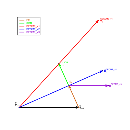
Figure 4: Illustration for One Iteration of the DECME Implementations.

Let $\{\theta_{t}-\tilde{\theta}_{t-1}\}$ represent the linear subspace spanned by $\theta_{t}-\tilde{\theta}_{t-1}$. SOR can be obtained by specifying $\mathscr{V}_{t}=\theta_{t}+\{\theta_{t}-\tilde{\theta}_{t-1}\}$ in the Dynamic CM-step of DECME, i.e., $\tilde{\theta}_{t}=\theta_{t}+\alpha_{t}d_{t}$, $d_{t}=\theta_{t}-\tilde{\theta}_{t-1}$, and $\alpha_{t}=\mathsf{argmax}_{\alpha}L(\theta_{t}+\alpha d_{t}|Y_{obs})$. The so-called relaxation factor $\alpha_{t}$ can be obtained by a line search. See Figure 4 for an illustration of the SOR iteration.

The reason that SOR may be used to accelerate EM is clear from the following theorem which implies that, in a small neighbourhood of the MLE, a point with larger likelihood value can always be found by enlarging the step size of EM:

Theorem 3.1

In a small neighbourhood of $\hat{\theta}$, the relaxation factor $\alpha_{t}$ of SOR is always positive.

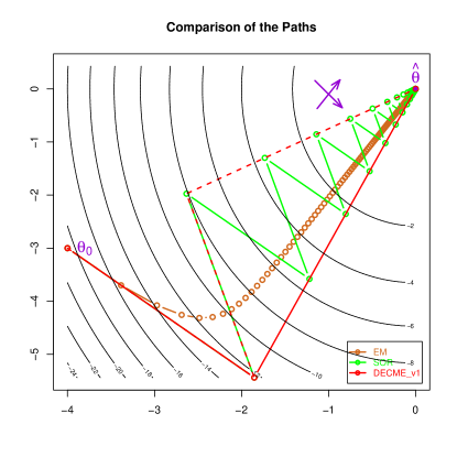
Figure 3: Comparison of the Paths of EM, SOR, and DECME_v1 for a Two-dimensional Example. The eigenvalues of $DM^{EM}$ are $0.9684$ and $0.6232$; the darkviolet cross on the upright corner shows the directions of the two eigenvectors of $DM^{EM}$; The red dashed lines represent the true path of DECME_v1 in its second iteration.

The proof is given in Appendix B and the conservative movement of EM is illustrated in Figure 3 for a two-dimensional simulated example. For simplicity, it has also been proposed to choose $\alpha_{t}$ as a fixed positive number (e.g., Lange, 1995). We call this version with fixed $\alpha_{t}$ the SORF method. Let $\lambda_{1}$ and $\lambda_{p}$ be the largest and smallest eigenvalues of $I_{com}^{-1}I_{obs}$ (see Appendix B for detailed discussion). It is well known that SORF achieves its optimal convergence rate $(\lambda_{1}-\lambda_{p})/(\lambda_{1}+\lambda_{p})$ if $\alpha_{t}=2/(\lambda_{1}+\lambda_{p})-1$ for any $t$ (see, e.g., Salakhutdinov and Roweis, 2003). In the past, the theoretical argument for SOR has been mainly based on this fact, which is obviously insufficient. The following theorem provides new angles for understanding the convergence of SOR.

Theorem 3.2

For a two-dimensional problem (i.e., $p=2$) and in a small neighbourhood of $\hat{\theta}$, the following results hold for SOR:

• $\alpha_{t}=\alpha_{t-2}$;

• SOR converges at least as fast as the optimal SORF, and the optimal SORF converges faster than EM; and

• SOR oscillates around the slowest converging direction of EM; The SOR estimates from the odd-numbered iterations lie on the same line and so do those from the even-numbered iterations; Furthermore, the two lines intersect at the MLE $\hat{\theta}$.

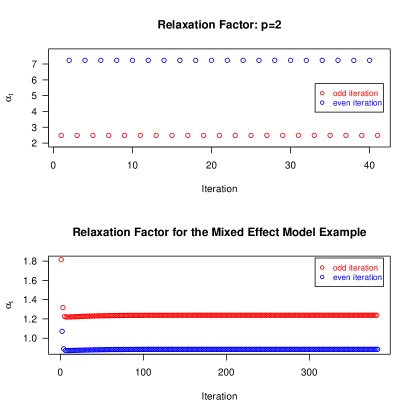
Figure 5: Relaxation Factor $\alpha_{t}$ Generated from SOR. The top panel plots the sequence of $\alpha_{t}$ for the two-dimensional example used to generate Figure 3, and the bottom panel plots the sequence of $\alpha_{t}$ from the simulated nine-dimensional example in Section 3.2 by using information from the linear mixed-effects model example in Section 2.1 and Section 4.2 .

The proof is provided in Appendix C. The zigzagging phenomena of SOR revealed by conclusion 3 is illustrated in Figure 3. For the case of $p>2$, it is interesting to see that the relaxation factors $\alpha_{t}$ generated from SOR also have a similar oscillating pattern as that for $p=2$ (conclusion 1). This is illustrated in Figure 5. The top panel of Figure 5 shows the relaxation factors for the two-dimensional example used to generate Figure 3 and the lower panel shows those for a nine-dimensional simulated example. The nine-dimensional example is generated by simulating the behaviour of EM in a small neighbourhood of the MLE for the linear mixed-effects model example in Section 2.1 and Section 4.2.

3.3 DECME_v1 and its Variants: Three Efficient DECME Implementations

3.3.1 The Basic Version: DECME_v1

The zigzagging problem has long been considered to be one of the major disadvantages for optimisation algorithms since the effective movement towards the MLE is usually small even if the step size is large. Figure 3 suggests a line search along the line connecting the zigzag points, as shown by one of the red dashed lines. For two-dimensional quadratic functions, this suggested procedure shown in Figure 3 converges immediately. Although this only represents a very rare case in practise, it motivated us to consider efficient DECME implementations.

One way to proceed is to repeat the procedure shown by the red dashed lines in Figure 3, i.e., each cycle of the new algorithm includes two iterations of SOR and a line search along the line connecting the initial point of the current cycle and the end point of the second SOR iteration. Numerical experiments show that this procedure is not very effective.

Another way to proceed is what we call DECME_v1. DECME_v1 retains the procedure shown by the red dashed lines in Figure 3 as its first two iterations and is formally defined as follows. At the first iteration of DECME_v1, $\tilde{\theta}_{1}$ is obtained by running one iteration of SOR from the starting point $\tilde{\theta}_{0}$. At the $t^{th}$ iteration of DECME_v1, one iteration of SOR is first conducted to obtain $\tilde{\theta}^{SOR}_{t}$, followed by a line search along the line connecting $\tilde{\theta}_{t-2}$ and $\tilde{\theta}^{SOR}_{t}$ to obtain $\tilde{\theta}_{t}$. The process is continued for $p$ iterations and restarted with a standard SOR iteration. The reason for restarting becomes clear from Theorem 3.3 below, which shows that DECME_v1 is equivalent to a conjugate direction method.

Formally, DECME_v1 is described in the framework of the generic DECME algorithm by implementing the Dynamic CM-step with two line searches as follows (except for the iterations where the algorithm is restarted):

• Dynamic CM-step of DECME_v1: the $t^{th}$ iteration

  • Substep 1: Calculate $\tilde{\theta}^{SOR}_{t}=\theta_{t}+\alpha_{t}^{(1)}d_{t}^{(1)}$, where $d_{t}^{(1)}=\theta_{t}-\tilde{\theta}_{t-1}$, and $\alpha_{t}^{(1)}=\mathsf{argmax}_{\alpha}L(\theta_{t}+\alpha d_{t}^{(1)}|Y_{obs})$;

  • Substep 2: Calculate $\tilde{\theta}_{t}=\tilde{\theta}^{SOR}_{t}+\ \alpha_{t}^{(2)}d_{t}^{(2)}$, where $d_{t}^{(2)}=\tilde{\theta}^{SOR}_{t}-\tilde{\theta}_{t-2}$, and $\alpha_{t}^{(2)}=\mathsf{argmax}_{\alpha}L(\tilde{\theta}^{SOR}_{t}+\alpha d_{t}^{(2)}|Y_{obs})$.

An illustration of the DECME_v1 iteration is given in Figure 4. We note that $\tilde{\theta}_{t}$ is actually the point that maximises $L(\theta|Y_{obs})$ over the two-dimensional subspace $\mathscr{V}_{t}=\tilde{\theta}_{t-1}+\{\tilde{\theta}_{t-1}-\tilde{\theta}_{t-2},\ \theta_{t}-\tilde{\theta}_{t-1}\}$ under certain conditions. This can be seen from the proof, given in Appendix D, of the following theorem,which demonstrates the efficiency of DECME_v1.

Theorem 3.3

In a small neighbourhood of the MLE, DECME_v1 with exact line search is equivalent to the conjugate direction method AEM.

Theorem 3.3 implies that DECME_v1 is about as efficient as AEM near the MLE in terms of the number of iterations. As noted in Section 1, DECME_v1 is much easier to implement and can be made automatic for almost all EM algorithms, which typically have coded likelihood evaluation routines for debugging code and monitoring convergence. A line search method is needed for DECME_v1, but can be implemented once for all; whereas evaluation of the gradient vector of $L(\theta|Y_{\rm obs})$ required for AEM is problem specific and thus demands substantially more programming efforts. Note also that gradient evaluation can be expensive. For example, for comparing different methods in the optimisation literature, it is often to count one evaluation of the gradient vector as $p$ function evaluations, where $p$ stands for the dimensionality of the parameter space.

The idea behind DECME_v1 is very similar to the parallel tangent (PARTAN) method for accelerating the steepest descent method (Shah et al., 1964). PARTAN can be viewed as a particular implementation of the conjugate gradient method (Fletcher and Reeves, 1964), developed based on the method in Hestenes and Stiefel (1952) for solving linear systems. It is also worth noting that PARTAN has certain advantage over the conjugate gradient method as discussed in Luenberger (2003, p. 257). For example, the convergence of PARTAN is more reliable than the conjugate gradient method when inexact line search is used as is often the case in practise.

3.3.2 DECME_v2 and DECME_v3

DECME_v1 requires two line search steps in one iteration. DECME_v2 and DECME_v3, the two variants of DECME_v1 that require a single line search in each iteration, are obtained by specifying a one-dimensional acceleration subspace in the dynamic CM-step as $\mathscr{V}_{t}=\theta_{t}+\{\theta_{t}-\tilde{\theta}_{t-2}\}$ and $\mathscr{V}_{t}=\theta_{t}+\{\tilde{\theta}_{t-1}-\tilde{\theta}_{t-2}\}$, respectively. This is depicted in Figure 4.

There is no much difference among the three newly proposed methods and SOR in terms of programming since their main building blocks, the EM iteration and a line search scheme, are the same. However, SOR can hardly compete with the new methods for all the examples we have observed. Among the three new implementations, DECME_v1 usually uses the smallest number of iterations to converge while it obviously takes more time to run one DECME_v1 iteration. Hence when the cost of running a line search, determined mainly by the cost of computing the log-likelihood, is low relative to the cost of running one EM iteration, DECME_v2 and DECME_v3 may be more efficient than DECME_v1 in terms of CPU time. These points are shown by the examples in next section.

4 Numerical Examples

In this section we use four sets of numerical examples to compare the convergence speed of EM, SOR, DECME_v1, DECME_v2, and DECME_v3 in terms of both number of iterations and CPU time.

4.1 The Setting for the Numerical Experiments

The line search scheme for all the examples is implemented by making use of the optimize function in R. The detailed discussion about the configuration of the function and how to achieve line search for constrained problems with line search routines designed for unconstrained problems is given in Appendix E.

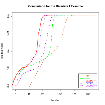
Figure 7: Comparison for the Bivariate $t$ Example in Section 4.4. Displayed are increases in $L(\theta|Y_{obs})$.

For the three examples in Section 4.2 (Section 2.1), 4.3 (Section 2.2), and 4.4, we first run EM with very stringent stopping criterions to obtain the maximum log-likelihood $l_{max}$ for each example. Then we run each of the five (nine for the example in Section 4.2) different algorithms from the same starting point and terminate them when $L(\theta|Y_{obs})$ is not less than $l_{max}-10^{-6}$. The results for these three examples, including number of iterations and CPU time, are summarised in Table 5 and 6. The increases in $L(\theta|Y_{obs})$ against the number of iteration for each of the three examples are shown in Figures 1, 2, 6 and 7. The setting and the results for the simulation study in Section 4.5 are slightly different.

4.2 The Linear Mixed-effects Model Example

The mixed-effects model example of Section 2.1 is used to illustrate the performance of DECME when applied to accelerate both EM and ECME. The increases of $L(\theta|Y_{obs})$ are shown in Figure 1 and 2. For this example, while EM needs $5,968$ iterations and SOR needs $918$ iterations to converge, all three new implementations of DECME needs no more than 170 iterations with only 104 iterations for DECME_v1. In terms of CPU time all three new methods converge about 30 times faster than EM. It is also interesting to see that the new methods works very well for accelerating ECME (especially DECME_v1 further reduces the number of iterations from 20 to 9) even when ECME already converges much faster than EM.

4.3 The Factor Analysis Model Example

The factor analysis example of Section 2.2 and the same starting point used in Liu and Rubin (1998) are used here. The increases of $L(\theta|Y_{obs})$ are shown in Figure 6. For this example, while all three new implementations of DECME converges much faster than EM and SOR, DECME_v1 uses only less than 1% of the number of iterations of EM (55 to 6,672) and is about 30 times faster than EM in terms of CPU time (1.2 seconds vs. 33.4 seconds). It is also interesting to see that all three new methods pass the flat period shown in Figure 6 much more quickly than both EM and SOR. As discussed in Liu and Rubin (1998), the long flat period of EM and SOR before convergence makes it difficult to assess the convergence. Clearly, this does not appear to be a problem for the three new methods.

4.4 A Bivariate $t$ Example

Let $t_{p}(\mu,\Psi,\nu)$ represent a multivariate $t$ distribution with $\mu$, $\Psi$, and $\nu$ as the mean, the covariance matrix, and the degree of freedom, respectively. Finding the MLE of the parameters $(\mu,\Psi,\nu)$ is a well known interesting application of the EM-type algorithms.

Here we use the bivariate $t$ distribution example in Liu and Rubin (1994), where the data is adapted from Table 1 of Cohen et al. (1993). Figure 7 shows the increases of $L(\theta|Y_{obs})$ for each algorithm starting from the same point $(\mu,\Psi,\nu)=((0,0)^{\prime},\mathsf{diag}(1,1),1)$. For this example, EM converges relatively fast with 293 iterations and 1.4 seconds. But we still see the advantage of the new implementations of DECME over EM and SOR: DECME_v1 uses only 32 iterations and 0.9 second to converge. Also note that SOR uses 1.5 seconds to converge, which is slightly more than that of EM.

4.5 Gaussian Mixture Examples

The EM algorithm is wildly acknowledged as a powerful method for fitting the mixture models, which are popular in many different areas such as machine learning and pattern recognition (e.g., Jordan and Jacobs, 1994; McLachlan and Krishnan, 1997; McLachlan and Peel, 2000; Bishop, 2006). While the slow convergence of EM has been frequently reported for fitting mixture models, a few extensions have been proposed for specifically accelerating this EM application (Liu and Sun, 1997; Dasgupta and Schulman, 2000; Celeux et al., 2001; Pilla and Lindsay, 2001, among others). Here we show that DECME, as an off-the-shelf accelerator, can be easily applied to achieve dramatically faster convergence than EM.

A class of mixtures of two univariate normal densities is used to illustrate the relation between the efficiency of EM and the separation of the component populations in the mixture in Redner and Walker (1984). Specifically, the mixture has the form of

$$\begin{array}[]{rcl}p(x|\pi_{1},\pi_{2},\mu_{1},\mu_{2},\sigma_{1}^{2},\sigma_{2}^{2})&=&\pi_{1}p_{1}(x|\mu_{1},\sigma_{1}^{2})+\pi_{2}p_{2}(x|\mu_{2},\sigma_{2}^{2}),\\ p_{i}(x|\mu_{i},\sigma_{i}^{2})&=&\frac{1}{\sqrt{2\pi\sigma_{i}}}e^{-(x-\mu_{i})^{2}/2\sigma_{i}^{2}},\ i=1,2.\end{array}$$ (4)

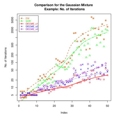
Figure 8: Comparison for the Gaussian Mixture Example in Section 4.5. Displayed are number of iterations; the smoothed curves are generated by robust local regression (Cleveland, 1979).

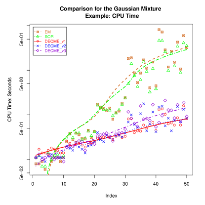
Figure 9: Comparison for the Gaussian Mixture Example in Section 4.5. Displayed are CPU time; the smoothed curves are generated by robust local regression.

Let $\pi_{1}=0.3,\ \pi_{2}=0.7,\ \sigma_{1}^{2}=\sigma_{2}^{2}=1$, and $\mu_{1}=-\mu_{2}$, then ten random samples of $1,000$ observations were generated from each case of $\mu_{1}-\mu_{2}=6,\ 4,\ 3,\ 2$ and $1.5$. We ran EM, SOR, DECME_v1, DECME_v2, and DECME_v3 from the same starting point $\pi_{1}^{(0)}=\pi_{2}^{(0)}=0.5,\ \sigma_{i}^{2^{(0)}}=0.5,\ \mu_{i}^{(0)}=1.5\mu_{i}$. The algorithms are terminated when $||\theta_{t+1}-\theta_{t}||_{1}\ <\ 10^{-5}$, where $||\cdot||_{1}$ represents the $l_{1}$ norm. The results for number of iterations and CPU time are shown in Figure 8 and Figure 9, respectively.

We see that SOR typically uses about half of the number of iterations of EM while the two have very similar performance in terms of CPU time. When EM converges very slowly, the three new implementations of DECME can be dramatically faster than EM with a factor 100 or more in terms of number of iterations and a factor of 50 or more in terms of CPU time. When EM converges very fast, from Figure 9, we see some overlapping among several methods in terms of CPU time for the first group of ten simulations, although all the accelerators still outperform EM in terms of number of iterations. In practise, fast convergence like this is somewhat rare for EM. Notice that all the methods take less than one second to converge. Hence, this phenomenon of overlapping should not be used to dismiss the advantage of the accelerators. Nevertheless, this may serve as empirical evidence to support the idea of accelerating EM only after a few EM iterations have been conducted as suggested in Jamshidian and Jennrich (1993).

5 Discussion

The limitation of using fixed acceleration subspaces in ECME led to the idea of dynamically constructing the subspaces for the supplementary $ML$-steps. We formulated this idea as the generic DECME algorithm, which provides a simple framework for developing stable and efficient acceleration methods of EM. The zigzagging problem of SOR, a special case of DECME, motivated the development of the three new DECME implementations, i.e., DECME_v1-v3. The stability of DECME is guaranteed by the nested EM iteration. The equivalence of DECME_v1 to AEM, a conjugate direction method, provides theoretical justification for the fast convergence of the new methods, which is also supported by the numerical results. Moreover, the simplicity of the new methods makes them more attractive than AEM.

In optimisation literature, it is popular to analyse the convergence of optimisation algorithms near the optimum with the assumption of an ideal exact line search. However, exact line search is not a realistic choice in practise (see the discussion in Appendix E). Hence, the relative performance of DECME_v1 and AEM, in both efficiency and stability, could be very different, especially when the starting point is far from the MLE. Note also that many works have been done to expedite the line search for SOR, e.g., Salakhutdinov and Roweis (2003) and Hesterberg (2005). It will be interesting to see how the similar techniques perform for DECME for we have shown that the newly proposed acceleration directions work much better than that used by SOR.

Our main focus in the current paper has been on accelerating EM. However, it is noteworthy that the proof of Theorem 3.3 only depends on the linear convergence rate of the underlying algorithm being accelerated rather than its specific structure. Hence an immediate point to make is that the new methods should also work for other EM-type algorithms of linear convergence rate or more broadly for the MM algorithm (Hunter and Lange, 2004). We leave this problem open for future investigation.

Appendix

Appendix A The Linear Convergence Rate of EM: a Quick Review

This section reviews some well known convergence properties of EM to establish necessary notations. These results are mainly adapted from Dempster et al. (1977) and Meng and Rubin (1994).

In a small neighbourhood of the MLE, the observed log-likelihood $L(\theta|Y_{obs})$ may be assumed to be a quadratic function:

$$L(\theta|Y_{obs})=-\frac{1}{2}(\theta-\hat{\theta})^{\prime}I_{obs}(\theta-\hat{\theta}).$$ (5)

Under this assumption, Dempster et al. (1977) proved that EM has a linear convergence rate determined by $DM^{EM}$, i.e., equation (1). We mentioned previously that $DM^{EM}$ is called the missing information fraction. It is named after the following identity:

$$DM^{EM}=I_{p}-I_{com}^{-1}I_{obs}=I_{com}^{-1}I_{mis},$$ (6)

where $I_{p}$ represents the identity matrix of order $p$, $I_{obs}$ and $I_{com}$ are the negative Hessian matrices of $L(\theta|Y_{obs})$ and $Q(\theta|Y_{obs},\hat{\theta})$ at the MLE, and $I_{mis}=I_{com}-I_{obs}$. The matrices $I_{obs}$, $I_{mis}$ and $I_{com}$ are usually called observed-data, missing-data, and complete-data information matrices. We assume that these matrices are positive definite in this paper.

Since $I_{com}$ is positive definite, there exists a positive definite matrix, denoted by $I_{com}^{1/2}$, such that $I_{com}=I_{com}^{1/2}I_{com}^{1/2}$. Further denote by $I_{com}^{-1/2}$ the inverse of $I_{com}^{1/2}$. Then $I_{com}^{-1}I_{obs}$ is similar to $I_{com}^{1/2}\times I_{com}^{-1}I_{obs}\times I_{com}^{-1/2}=I_{com}^{-1/2}I_{obs}I_{com}^{-1/2}$ and, thereby, $I_{com}^{-1}I_{obs}$ and $I_{com}^{-1/2}I_{obs}I_{com}^{-1/2}$ have the same eigenvalues. Since $I_{com}^{-1/2}I_{obs}I_{com}^{-1/2}$ is symmetric, there exists an orthogonal matrix $T$ such that

$$I_{com}^{-1/2}I_{obs}I_{com}^{-1/2}=T\Lambda T^{{}^{\prime}},$$ (7)

where $\Lambda=\mathsf{diag}(\lambda_{1},\cdots,\lambda_{p})$, and $\lambda_{i},\ i=1,\cdots,p$, are the eigenvalues of $I_{com}^{-1}I_{obs}$. Therefore,

$$I_{com}^{-1}I_{obs}=I_{com}^{-1/2}T\Lambda T^{{}^{\prime}}I_{com}^{1/2}.$$ (8)

Let $P=I_{com}^{-1/2}T$, then we have $I_{com}^{-1}I_{obs}=P\Lambda P^{-1}$. Furthermore, the columns of $P$ and the rows of $P^{-1}$ are eigenvectors of $I_{com}^{-1}I_{obs}$ and $I_{obs}I_{com}^{-1}$, respectively. Define $\eta=P^{-1}(\hat{\theta}-\theta)$, then from equation (1) we have $\eta_{t}=(I_{p}-\Lambda)\eta_{t-1}$, or equivalently

$$\eta_{t,i}=(1-\lambda_{i})\eta_{t-1,i},\ i=1,\cdots,p.$$ (9)

Equation (9) implies that EM converges independently along the $p$ eigenvector directions of $I_{com}^{-1}I_{obs}$ (or equivalently $DM^{EM}$) with the rates determined by the corresponding eigenvalues. For simplicity of the later discussion, we assume $1>\lambda_{1}>\lambda_{2}>\cdots>\lambda_{p}>0$ and $\eta_{0,i}\neq 0,\ i=1,\cdots,p$.

Appendix B The Conservative Step Size of EM: Proof of Theorem 3.1

From equation (5) and the definition of SOR in Section 3.2, it is easy to show that

$$\alpha_{t}=\frac{(\theta_{t}-\tilde{\theta}_{t-1})^{\prime}I_{obs}({\hat{\theta}}-\theta_{t})}{(\theta_{t}-\tilde{\theta}_{t-1})^{\prime}I_{obs}(\theta_{t}-\tilde{\theta}_{t-1})}.$$ (10)

Then making use of the fact that $\theta_{t}=\theta_{t-1}+I_{com}^{-1}I_{obs}(\hat{\theta}-\theta_{t-1})$ (followed from equations 1 and 6) leads to

$$\alpha_{t}=\frac{({\hat{\theta}}-\tilde{\theta}_{t-1})^{\prime}I_{obs}I_{com}^{-1}I_{obs}({\hat{\theta}}-\tilde{\theta}_{t-1})}{({\hat{\theta}}-\tilde{\theta}_{t-1})^{\prime}I_{obs}I_{com}^{-1}I_{obs}I_{com}^{-1}I_{obs}({\hat{\theta}}-\tilde{\theta}_{t-1})}-1.$$ (11)

By definition of $\eta$, we have ${\hat{\theta}}-\tilde{\theta}_{t-1}=I_{com}^{-1/2}T\tilde{\eta}_{t-1}$. Making use of equation (7) and the fact that $T$ is an orthogonal matrix yields

$$\alpha_{t}=\frac{\tilde{\eta}_{t-1}^{\prime}\Lambda^{2}\tilde{\eta}_{t-1}}{\tilde{\eta}_{t-1}^{\prime}\Lambda^{3}\tilde{\eta}_{t-1}}-1.$$ (12)

Since $\Lambda$ is diagonal and all its diagonal elements are between $0$ and $1$, it follows immediately that $\alpha_{t}>0$. $\Box$

Appendix C The Convergence of SOR: Proof of Theorem 3.2

Similar to equation (1) and (9) for EM, we have the following results for SOR:

$$\hat{\theta}-\tilde{\theta}_{t}=[I_{p}-(1+\alpha_{t})I_{com}^{-1}I_{obs}](\hat{\theta}-\tilde{\theta}_{t-1}),$$ (13)

and

$$\tilde{\eta}_{t,i}=[1-(1+\alpha_{t})\lambda_{i}]\tilde{\eta}_{t-1,i}\ ,\ \ i=1,\cdots,p.$$ (14)

For $p=2$, from equation (12), we have

$$\alpha_{t}=\frac{\lambda_{1}^{2}\tilde{\eta}_{t-1,1}^{2}+\lambda_{2}^{2}\tilde{\eta}_{t-1,2}^{2}}{\lambda_{1}^{3}\tilde{\eta}_{t-1,1}^{2}+\lambda_{2}^{3}\tilde{\eta}_{t-1,2}^{2}}-1,$$ (15)

and then,

$$1-(1+\alpha_{t})\lambda_{1}=\frac{\lambda_{2}^{2}(\lambda_{2}-\lambda_{1})\tilde{\eta}_{t-1,2}^{2}}{\lambda_{1}^{3}\tilde{\eta}_{t-1,1}^{2}+\lambda_{2}^{3}\tilde{\eta}_{t-1,2}^{2}},\ 1-(1+\alpha_{t})\lambda_{2}=\frac{\lambda_{1}^{2}(\lambda_{1}-\lambda_{2})\tilde{\eta}_{t-1,1}^{2}}{\lambda_{1}^{3}\tilde{\eta}_{t-1,1}^{2}+\lambda_{2}^{3}\tilde{\eta}_{t-1,2}^{2}}.$$ (16)

From equation (14) and equation (16), we have

$$\frac{\tilde{\eta}_{t,1}}{\tilde{\eta}_{t,2}}=-\frac{\lambda_{2}^{2}}{\lambda_{1}^{2}}\frac{\tilde{\eta}_{t-1,2}}{\tilde{\eta}_{t-1,1}}.$$ (17)

It follows that $\tilde{\eta}_{t,1}/\tilde{\eta}_{t,2}=\eta_{t-2,1}/\tilde{\eta}_{t-2,2}.$ Furthermore, from equation (15), we have

$$\alpha_{t}=\frac{\lambda_{1}^{2}(\tilde{\eta}_{t-1,1}/\tilde{\eta}_{t-1,2})^{2}+\lambda_{2}^{2}}{\lambda_{1}^{3}(\tilde{\eta}_{t-1,1}/\tilde{\eta}_{t-1,2})^{2}+\lambda_{2}^{3}}-1,$$ (18)

and immediately $\alpha_{t}=\alpha_{t-2}$, which proves conclusion 1.

Now define a trivial algorithm, called SOR2, where each iteration of SOR2 includes two iterations of SOR. From equation (13), we have

$$\hat{\theta}-\tilde{\theta}_{t+1}=[I_{2}-(1+\alpha_{t})I_{com}^{-1}I_{obs}][I_{2}-(1+\alpha_{t-1})I_{com}^{-1}I_{obs}](\hat{\theta}-\tilde{\theta}_{t-1}).$$ (19)

By conclusion 1, $[I_{p}-(1+\alpha_{t})I_{com}^{-1}I_{obs}][I_{p}-(1+\alpha_{t-1})I_{com}^{-1}I_{obs}]$ is a constant matrix and denote it by $DM^{SOR2}$, which obviously determines the convergence rate of SOR2. By using equation (8), we have $DM^{SOR2}=I_{com}^{-1/2}T[I_{p}-(1+\alpha_{t})\Lambda][I_{p}-(1+\alpha_{t-1})\Lambda]T^{\prime}I_{com}^{1/2}$. Moreover, with equation (17) and (18), it is easy to show that

$$[1-(1+\alpha_{t})\lambda_{j}][1-(1+\alpha_{t-1})\lambda_{j}]=\frac{(\lambda_{2}-\lambda_{1})^{2}}{\lambda_{1}^{2}+\lambda_{2}^{2}+\lambda_{1}\lambda_{2}\left(\frac{\lambda_{1}^{2}}{\lambda_{2}^{2}}\frac{\tilde{\eta}_{t-1,1}^{2}}{\tilde{\eta}_{t-1,2}^{2}}+\frac{\lambda_{2}^{2}}{\lambda_{1}^{2}}\frac{\tilde{\eta}_{t-1,2}^{2}}{\tilde{\eta}_{t-1,1}^{2}}\right)},\ j=1,2.$$ (20)

It follows that $DM^{SOR2}=[1-(1+\alpha_{t})\lambda_{1}][1-(1+\alpha_{t-1})\lambda_{1}]I_{2}$, which means SOR2 converges with the same rate $[1-(1+\alpha_{t})\lambda_{1}][1-(1+\alpha_{t-1})\lambda_{1}]$ along any direction. From equation (20), it is easy to see that

$$[1-(1+\alpha_{t})\lambda_{1}][1-(1+\alpha_{t-1})\lambda_{1}]\leq\frac{(\lambda_{1}-\lambda_{2})^{2}}{(\lambda_{1}+\lambda_{2})^{2}}=(1-\frac{2\lambda_{2}}{\lambda_{1}+\lambda_{2}})^{2}<(1-\lambda_{2})^{2}.$$

Note that $(\lambda_{1}-\lambda_{2})/(\lambda_{1}+\lambda_{2})$ is the optimal convergence rate of SORF and that $1-\lambda_{2}$ is the convergence rate of EM. Hence conclusion 2 follows.

Since $\lambda_{1}>\lambda_{2}$, equation (16) implies that $1-(1+\alpha_{t})\lambda_{1}<0$ and $1-(1+\alpha_{t})\lambda_{2}>0$. So from equation (14), we have $\tilde{\eta}_{t,1}\tilde{\eta}_{t-1,1}<0$ and $\tilde{\eta}_{t,2}\tilde{\eta}_{t-1,2}>0$. This proves the first statement in conclusion 3. Note that $\tilde{\theta}_{t+1}-\tilde{\theta}_{t}=(I-DM^{SOR2})(\hat{\theta}-\tilde{\theta}_{t-1})\propto\hat{\theta}-\tilde{\theta}_{t-1}$. Hence $\tilde{\theta}_{t+1}-\tilde{\theta}_{t-1}$ is parallel to $\hat{\theta}-\tilde{\theta}_{t-1}$, which concludes the second statement in conclusion 3. $\Box$

Appendix D The Convergence of DECME_v1: Proof of Theorem 3.3

We prove this by induction. This version of proof is similar to the proof of the PARTAN theorem in Luenberger (2003, pp. 255-256). However, the difference between a generalised gradient direction and the gradient direction should be taken into account.

It is certainly true for $t=1$ since the first iteration is a line search along the EM direction for both DECME_v1 and AEM.

Now suppose that $\tilde{\theta}_{0},\tilde{\theta}_{1},\cdots,\tilde{\theta}_{t-1}$ have been generated by AEM and $\tilde{\theta}_{t}$ is determined by DECME_v1. We want to show that $\tilde{\theta}_{t}$ is the same point as that generated by another iteration of AEM. For this to be true $\tilde{\theta}_{t}$ must be the point that maximises $L(\theta|Y_{obs})$ over the two-dimensional plane $\tilde{\theta}_{t-1}+\{\tilde{\theta}_{t-1}-\tilde{\theta}_{t-2},\theta_{t}-\tilde{\theta}_{t-1}\}$. Since we assume that $L(\theta|Y_{obs})$ is a quadratic function with a positive definite Hessian matrix, $L(\theta|Y_{obs})$ is strictly convex and we only need to prove $\tilde{g}_{t}$ (gradient of $L(\theta|Y_{obs})$ at $\tilde{\theta}_{t}$) is orthogonal to $\tilde{\theta}_{t-1}-\tilde{\theta}_{t-2}$ and $\theta_{t}-\tilde{\theta}_{t-1}$, or equivalently $\tilde{\theta}^{SOR}_{t}-\tilde{\theta}_{t-2}$ and $\theta_{t}-\tilde{\theta}_{t-1}$. Since $\tilde{\theta}_{t}$ maximises $L(\theta|Y_{obs})$ along $\tilde{\theta}^{SOR}_{t}-\tilde{\theta}_{t-2}$, $\tilde{g}_{t}$ is orthogonal to $\tilde{\theta}^{SOR}_{t}-\tilde{\theta}_{t-2}$. Similarly, $\tilde{g}^{SOR}_{t}$ is orthogonal to $\theta_{t}-\tilde{\theta}_{t-1}$. Furthermore, we have $\tilde{g}^{\prime}_{t-2}(\theta_{t}-\tilde{\theta}_{t-1})=(\hat{\theta}-\tilde{\theta}_{t-2})^{\prime}I_{obs}I_{com}^{-1}I_{obs}(\hat{\theta}-\tilde{\theta}_{t-1})=(\theta_{t-1}-\tilde{\theta}_{t-2})^{\prime}\tilde{g}_{t-1}=0$, where the last identity is true due to the Expanding Subspace Theorem (Luenberger, 2003, p. 241) for the conjugate direction methods. Then $\tilde{g}^{\prime}_{t}(\theta^{SOR}_{t}-\tilde{\theta}_{t-1})=(\hat{\theta}-\tilde{\theta}_{t})^{\prime}I_{obs}(\theta^{SOR}_{t}-\tilde{\theta}_{t-1})=[\hat{\theta}-\tilde{\theta}_{t-2}-(1+\alpha_{t}^{(2)})(\tilde{\theta}^{SOR}_{t}-\tilde{\theta}_{t-2})]^{\prime}I_{obs}(\theta^{SOR}_{t}-\tilde{\theta}_{t-1})=[-\alpha_{t}^{(2)}(\hat{\theta}-\tilde{\theta}_{t-2})I_{obs}+(1+\alpha_{t}^{(2)})(\hat{\theta}-\tilde{\theta}^{SOR}_{t})^{\prime}I_{obs}]^{\prime}(\theta^{SOR}_{t}-\tilde{\theta}_{t-1})=[-\alpha_{t}^{(2)}\tilde{g}_{t-2}+(1+\alpha_{t}^{(2)})\tilde{g}^{SOR}_{t}]^{\prime}(\theta^{SOR}_{t}-\tilde{\theta}_{t-1})=0$. It follows that $\tilde{g}_{t}$ is orthogonal to $\theta^{SOR}_{t}-\tilde{\theta}_{t-1}$. $\Box$

Appendix E Implementation of Line Search

In practise, it is neither computationally feasible nor necessary to conduct exact line search. In fact we can often achieve higher efficiency by sacrificing accuracy in the line search routine, although the number of iterations may increase. There are various criterions for terminating the line search routine for a desirable trade-off (Luenberger, 2003, pp. 211-214) and different approaches have been proposed for efficient implementation of those criterions (Moré and Thuente, 1994). Furthermore, some transformations to transform constrained problems into unconstrained problems can be useful, as discussed in Salakhutdinov and Roweis (2003).

Here we take a different approach to implement the line search by taking the advantage of the fact that sometimes it is easy to figure out the feasible region of a constrained problem along a single line. After the feasible region is computed, many commonly used line search routines available in standard software can be easily applied. In our case the line search is conducted with the optimize function in R by passing the computed interval to the optimize function through its option interval =. Note that the interval computed in this way is usually very wide and some other information may be used to narrow it down for higher efficiency. For example, we can start the line search by forcing $\alpha>0$ for SOR. Furthermore, we control the accuracy of the line search by setting $tol=0.01$ in the optimize function. This choice is somehow arbitrary. One advantage is that the line search is forced to be more accurate when the algorithm approaches the MLE since the magnitude of the differences between consecutive estimates usually becomes smaller with the progress of the algorithm.

For the constraints involved in the examples, we summarise the methods to obtain the feasible region as follows. Denote the current estimation by $\theta$ and the search direction by $d$. Our goal is to find the feasible region of $\alpha$ (an interval including 0 for the examples used in this paper) for a univariate function $f(\theta+\alpha d)$. If there are several sets of constraints for one model, we can determine the feasible region induced by each of them and then take their intersection. Without loss of generality, we assume in the following that $d$ is the counterpart of the discussed parameters in the vector representing the search direction.

• The degree of freedom $\nu$ in the $t$ distribution. It is easy to compute the boundary for $\alpha$ such that $\nu+\alpha d>0$.

• The mixing coefficients, $\pi_{i},\ i=1,\cdots,K$, in the mixture model. There are two types of constraints here, i.e., $\sum_{i=1}^{K}\pi_{i}=1$ and $\pi_{i}\geq 0$. By using the first constraint, we only need to consider the first $K-1$ coefficients with constraints $\sum_{i=1}^{K-1}\pi_{i}\leq 1$ and $\pi_{i}\geq 0,\ i=1,\cdots,K-1$. Then we only need to find the intersection of the solutions for the inequalities $\sum_{i=1}^{K-1}\pi_{i}+\alpha\sum_{i=1}^{K-1}d_{i}\leq 1$ and $\pi_{i}+\alpha d_{i}\geq 0,\ i=1,\cdots,K-1$.

• The variance components in the linear mixed-effects model and the mixture model and the uniquenesses in the factor analysis model. This can be handled in the same way as that for the degree of freedom in the $t$ distribution.

• The covariance matrices in the linear mixed-effects model and the $t$ distribution. For the current paper, only two-dimensional covariance matrices are involved. A two-dimensional matrix $\Psi$ is positive definite if and only if $\Psi_{1,1}>0$ and $\det(\Psi)>0$. Hence we only need to guarantee $\Psi_{1,1}+\alpha d_{1,1}>0$ and $\det(\Psi+\alpha D)>0$ (assume $D$ is the matrix generated from the vector $d$ in the same way as $\Psi$ is generated from $\theta$). For other covariance matrices of fairly small size, similar method could be used. When the dimension of the covariance matrix is high, it is a common practise to enforce certain structure on the matrix. For example, in spatial statistics, the covariance matrices are usually assumed to be generated from various covariance functions with very few parameters (Zhang, 2002; Zhu et al., 2005; Zhang, 2007) and the feasible region of $\alpha$ can be easily obtained.

Table 1: Eigenvalues of $DM^{EM}$ and $DM^{ECME}$ for the Linear Mixed-effects Model Example in Section 2.1

Algorithm		Eigenvalues of the missing information fraction
EM		0.9860 0.9746 0.7888 0.6706 0.5176 0.3874 0.3260 0.2710 0.0364
ECME		0.5176 0.3874 0.3260 0.2710 0.0364 0.0000 0.0000 0.0000 0.0000

Table 2: The Four Largest Eigenvalues and the Corresponding Eigenvectors of $DM^{EM}$ for the Linear Mixed-effects Model Example in Section 2.1

Eigenvalue		Corresponding eigenvector
0.9860		(0.0000 0.0000 -0.0413 -0.9991 0.0000 0.0000 0.0000 0.0000 0.0000)
0.9746		(0.0413 0.9991 0.0000 0.0000 0.0000 0.0000 0.0000 0.0000 0.0000)
0.7888		(0.0000 0.0000 -0.0433 0.9991 0.0000 0.0000 0.0000 0.0000 0.0000)
0.6706		(-0.0433 0.9991 0.0000 0.0000 0.0000 0.0000 0.0000 0.0000 0.0000)

Table 3: The Ten Leading Eigenvalues of $DM^{EM}$ and $DM^{ECME}$ for the Factor Analysis Model Example in Section 2.2

Algorithm		Ten leading eigenvalues of the missing information fraction
EM		1-2E-12 0.9992 0.9651 0.9492 0.9318 0.8972 0.8699 0.8232 0.8197 0.7876
ECME-1		1-2E-12 0.9979 0.9509 0.9292 0.9124 0.8725 0.8480 0.8031 0.7877 0.7539
ECME-2		0.9987 0.8715 0.7321 0.6673 0.5184 0.4770 0.4496 0.3727 0.3369 0.0000

Table 4: The Two Largest Eigenvalues and the Corresponding Eigenvectors of $DM^{EM}$ for the Factor Analysis Model Example in Section 2.2

Eigenvalue		Corresponding eigenvector
1-2E-12		0.0812 0.0934 -0.4897 -0.1335 0.0684 0.0748 0.0363 -0.0864 -0.0949
		0.0996 0.1288 0.7171 0.1962 0.1085 0.1138 0.0954 0.2099 0.2047
		0.0000 0.0000 0.0000 0.0000 0.0000 0.0000 0.0000 0.0000 0.0000
		0.0000 0.0000 0.0000 0.0000 0.0000 0.0000 0.0000 0.0000 0.0000
0.9992		0.0046 0.0057 -0.0047 -0.0005 -0.0047 -0.0034 -0.0038 -0.0013 0.0005
		-0.0062 -0.0071 -0.0092 -0.0064 0.0053 0.0060 0.0045 0.0049 0.0034
		0.0267 0.0441 -0.2871 0.0013 -0.0103 -0.0177 -0.0106 -0.0139 -0.0144
		-0.0028 0.0079 -0.9557 0.0111 0.0013 0.0040 -0.0011 -0.0028 0.0006

Table 5: Comparison of Convergence for the Three Examples in Section 4.2, 4.3, and 4.4

		Number of iterations
Example		EM		ECME		SOR		DECME_v1		DECME_v2		DECME_v3
Mixed effect: EM		5,968		$\diagup$		918		104		133		166
Mixed effect: ECME		$\diagup$		20		15		9		13		15
Factor analysis		6,672		$\diagup$		1,698		55		91		150
Bivariate $t$		293		$\diagup$		96		32		48		63

Table 6: Comparison of Convergence for the Three Examples in Section 4.2, 4.3, and 4.4, cont’d

		CPU time (s)
Example		EM		ECME		SOR		DECME_v1		DECME_v2		DECME_v3
Mixed effect: EM		518.9		$\diagup$		110.9		15.7		15.6		19.3
Mixed effect: ECME		$\diagup$		1.8		1.8		1.3		1.6		1.8
Factor analysis		33.4		$\diagup$		21.3		1.2		1.3		2.0
Bivariate $t$		1.4		$\diagup$		1.5		0.9		0.9		1.1

Figure 1: Comparison for the Linear Mixed-effects Model Example in Section 2.1 and Section 4.2. Displayed are increases in $L(\theta|Y_{obs})$.

Figure 6: Comparison for the Factor Analysis Model Example in Section 2.2 and 4.3. Displayed are increases in $L(\theta|Y_{obs})$.

References

- Bishop (2006) Bishop, C. M. (2006). Pattern recognition and machine learning. Information Science and Statistics. New York: Springer.
- Celeux et al. (2001) Celeux, G., S. Chrétien, F. Forbes, and A. Mkhadri (2001). A component-wise EM algorithm for mixtures. J. Comput. Graph. Statist. 10(4), 697–712.
- Cleveland (1979) Cleveland, W. S. (1979). Robust locally weighted regression and smoothing scatterplots. Journal of the American Statistical Association 74, 829–836.
- Cohen et al. (1993) Cohen, M., S. R. Dalal, and J. W. Tukey (1993). Robust, smoothly heterogeneous variance regression. Journal of the Royal Statistical Society, Series C: Applied Statistics 42, 339–353.
- Concus et al. (1976) Concus, P., G. H. Golub, and D. P. O’Leary (1976). A generalized conjugate gradient method for the numerical solution of elliptic partial differential equations. In Sparse matrix computations (Proc. Sympos., Argonne Nat. Lab., Lemont, Ill., 1975), pp. 309–332. New York: Academic Press.
- Dasgupta and Schulman (2000) Dasgupta, S. and L. J. Schulman (2000). A two-round variant of em for gaussian mixtures. In UAI ’00: Proceedings of the 16th Conference on Uncertainty in Artificial Intelligence, San Francisco, CA, USA, pp. 152–159. Morgan Kaufmann Publishers Inc.
- Dempster et al. (1977) Dempster, A. P., N. M. Laird, and D. B. Rubin (1977). Maximum likelihood from incomplete data via the EM algorithm. Journal of the Royal Statistical Society, Series B: Methodological 39, 1–22.
- Fletcher and Reeves (1964) Fletcher, R. and C. M. Reeves (1964). Function minimization by conjugate gradients. Comput. J. 7, 149–154.
- Frankel (1950) Frankel, S. (1950). Convergence rates of iterative treatments of partial differential equations. Mathematical Tables and Other Aids to Computation 4(30), 65–75.
- Gelfand et al. (1990) Gelfand, A. E., S. E. Hills, A. Racine-Poon, and A. F. M. Smith (1990). Illustration of Bayesian inference in normal data models using Gibbs sampling. Journal of the American Statistical Association 85, 972–985.
- Golub and Nash (1982) Golub, G. H. and S. G. Nash (1982). Nonorthogonal analysis of variance using a generalized conjugate-gradient algorithm. J. Amer. Statist. Assoc. 77(377), 109–116.
- Hestenes and Stiefel (1952) Hestenes, M. R. and E. Stiefel (1952). Methods of conjugate gradients for solving linear systems. J. Research Nat. Bur. Standards 49, 409–436 (1953).
- Hesterberg (2005) Hesterberg, T. (2005). Staggered Aitken acceleration for EM. In ASA Proceedings of the Joint Statistical Meetings, pp. 2101–2110. American Statistical Association.
- Hunter and Lange (2004) Hunter, D. and K. Lange (2004). A Tutorial on MM Algorithms. The American Statistician 58(1), 30–38.
- Jamshidian and Jennrich (1993) Jamshidian, M. and R. I. Jennrich (1993). Conjugate gradient acceleration of the em algorithm. Journal of the American Statistical Association 88(421), 221–228.
- Jordan and Jacobs (1994) Jordan, M. I. and R. A. Jacobs (1994). Hierarchical mixtures of experts and the em algorithm. Neural Computation 6, 181–214.
- Jöreskog (1969) Jöreskog, K. (1969, June). A general approach to confirmatory maximum likelihood factor analysis. Psychometrika 34(2), 183–202.
- Kowalski et al. (1997) Kowalski, J., X. Tu, R. Day, and J. Mendoza-Blanco (1997). On the rate of convergence of the ECME algorithm for multiple regression models with t-distributed errors. Biometrika 84(2), 269.
- Laird and Ware (1982) Laird, N. M. and J. H. Ware (1982). Random-effects models for longitudinal data. Biometrics 38, 963–974.
- Lange (1995) Lange, K. (1995). A gradient algorithm locally equivalent to the EM algorithm. J. Roy. Statist. Soc. Ser. B 57(2), 425–437.
- Liu (1998) Liu, C. (1998). Information matrix computation from conditional information via normal approximation. Biometrika 85, 973–979.
- Liu and Rubin (1994) Liu, C. and D. B. Rubin (1994). The ECME algorithm: A simple extension of EM and ECM with faster monotone convergence. Biometrika 81, 633–648.
- Liu and Rubin (1998) Liu, C. and D. B. Rubin (1998). Maximum likelihood estimation of factor analysis using the ECME algorithm with complete and incomplete data. Statist. Sinica 8(3), 729–747.
- Liu and Sun (1997) Liu, C. and D. X. Sun (1997). Acceleration of EM algorithm for mixture models using ECME. In ASA Proceedings of the Statistical Computing Section, pp. 109–114. American Statistical Association.
- Luenberger (2003) Luenberger, D. (2003). Linear and Nonlinear Programming (2nd ed.). Springer.
- McLachlan and Peel (2000) McLachlan, G. and D. Peel (2000). Finite mixture models. Wiley Series in Probability and Statistics: Applied Probability and Statistics. Wiley-Interscience, New York.
- McLachlan and Krishnan (1997) McLachlan, G. J. and T. Krishnan (1997). The EM algorithm and extensions. Wiley Series in Probability and Statistics: Applied Probability and Statistics. New York: John Wiley & Sons Inc. A Wiley-Interscience Publication.
- Meng and Rubin (1993) Meng, X. and D. B. Rubin (1993). Maximum likelihood estimation via the ECM algorithm: A general framework. Biometrika 80, 267–278.
- Meng and Rubin (1994) Meng, X. and D. B. Rubin (1994). On the global and componentwise rates of convergence of the EM algorithm (STMA V36 1300). Linear Algebra and its Applications 199, 413–425.
- Meng and van Dyk (1997) Meng, X. and D. van Dyk (1997). The EM algorithm – An old folk-song sung to a fast new tune (Disc: P541-567). Journal of the Royal Statistical Society, Series B: Methodological 59, 511–540.
- Moré and Thuente (1994) Moré, J. J. and D. J. Thuente (1994). Line search algorithms with guaranteed sufficient decrease. ACM Trans. Math. Software 20(3), 286–307.
- Pilla and Lindsay (2001) Pilla, R. S. and B. G. Lindsay (2001). Alternative EM methods for nonparametric finite mixture models. Biometrika 88(2), 535–550.
- Pinheiro et al. (2001) Pinheiro, J. C., C. Liu, and Y. Wu (2001). Efficient algorithms for robust estimation in linear mixed-effects models using the multivariate t distribution. Journal of Computational and Graphical Statistics 10(2), 249–276.
- R Development Core Team (2008) R Development Core Team (2008). R: A Language and Environment for Statistical Computing. Vienna, Austria: R Foundation for Statistical Computing. ISBN 3-900051-07-0.
- Redner and Walker (1984) Redner, R. A. and H. F. Walker (1984). Mixture densities, maximum likelihood and the EM algorithm. SIAM Review 26, 195–202.
- Rubin and Thayer (1982) Rubin, D. B. and D. T. Thayer (1982). EM algorithms for ML factor analysis. Psychometrika 47, 69–76.
- Salakhutdinov and Roweis (2003) Salakhutdinov, R. and S. Roweis (2003). Adaptive overrelaxed bound optimization methods. In In Proceedings of International Conference on Machine Learning, ICML. International Conference on Machine Learning, ICML, pp. 664–671.
- Sammel and Ryan (1996) Sammel, M. and L. Ryan (1996). Latent variable models with fixed effects. Biometrics 52(2), 650–663.
- Shah et al. (1964) Shah, B. V., R. J. Buehler, and O. Kempthorne (1964). Some algorithms for minimizing a function of several variables. J. Soc. Indust. Appl. Math. 12, 74–92.
- Varadhan and Roland (2008) Varadhan, R. and C. Roland (2008). Simple and globally convergent methods for accelerating the convergence of any EM algorithm. Scand. J. Statist. 35(2), 335–353.
- Wu (1983) Wu, C. F. J. (1983). On the convergence properties of the EM algorithm. The Annals of Statistics 11, 95–103.
- Young (1954) Young, D. (1954). Iterative methods for solving partial difference equations of elliptic type. Transactions of the American Mathematical Society 76(1), 92–111.
- Zhang (2002) Zhang, H. (2002). On estimation and prediction for spatial generalized linear mixed models. Biometrics 58(1), 129–136.
- Zhang (2007) Zhang, H. (2007). Maximum-likelihood estimation for multivariate spatial linear coregionalization models. EnvironMetrics 18(2), 125–139.
- Zhu et al. (2005) Zhu, J., J. C. Eickhoff, and P. Yan (2005). Generalized linear latent variable models for repeated measures of spatially correlated multivariate data. Biometrics 61(3), 674–683.