Aharonov-Bohm Effect and High-Velocity Estimates of Solutions to the Schrödinger Equation

To Mario Castagnino on the occasion of his 75th birthday.

Abstract

The Aharonov-Bohm effect is a fundamental issue in physics that has been extensively studied in the literature and is discussed in most of the textbooks in quantum mechanics. The issues at stake are what are the fundamental electromagnetic quantities in quantum physics, if magnetic fields can act at a distance on charged particles and if the magnetic potentials have a real physical significance. The Aharonov-Bohm effect is a very controversial issue. From the experimental side the issues were settled by the remarkable experiments of Tonomura et al. [Observation of Aharonov-Bohm effect by electron holography, Phys. Rev. Lett. 48 (1982) 1443-1446 , Evidence for Aharonov-Bohm effect with magnetic field completely shielded from electron wave, Phys. Rev. Lett. 56 (1986) 792-795] with toroidal magnets that gave a strong experimental evidence of the physical existence of the Aharonov-Bohm effect, and by the recent experiment of Caprez et al. [“Macroscopic test of the Aharonov-Bohm effect,” Phys. Rev. Lett. 99 (2007) 210401] that shows that the results of the Tonomura et al. experiments can not be explained by the action of a force. Aharonov and Bohm [Significance of electromagnetic potentials in the quantum theory, Phys. Rev. 115 (1959) 485-491 ] proposed an Ansatz for the solution to the Schrödinger equation in simply connected regions of space where there are no electromagnetic fields. It consists of multiplying the free evolution by the Dirac magnetic factor. The Aharonov-Bohm Ansatz predicts the results of the experiments of Tonomura et al. and of Caprez et al.. Recently in [M. Ballesteros, R. Weder, The Aharonov-Bohm effect and Tonomura et al. experiments: Rigorous results, J. Math. Phys. 50 (2009) 122108] we gave the first rigorous proof that the Aharonov-Bohm Ansatz is a good approximation to the exact solution for toroidal magnets under the conditions of the experiments of Tonomura et al.. We provided a rigorous, simple, quantitative, error bound for the difference in norm between the exact solution and the Aharonov-Bohm Ansatz. In this paper we prove that these results do not depend on the particular geometry of the magnets and on the velocities of the incoming electrons used on the experiments, and on the gaussian shape of the wave packets used to obtain our quantitative error bound. We consider a general class of magnets that are a finite union of handle bodies. Each handle body is diffeomorphic to a torus or a ball, and some of them can be patched though the boundary. We formulate the Aharonov-bohm Ansatz that is appropriate to this general case and we prove that the exact solution to the Schrödinger equation is given by the Aharonov-Bohm Ansatz up to an error bound in norm that is uniform in time and that decays as a constant divided by $v^{\rho},0<\rho<1$, with $v$ the velocity. The results of Tonomura et al., of Caprez et al., our previous results and the results of this paper give a firm experimental and theoretical basis to the existence of the Aharonov-Bohm effect and to its quantum nature. Namely, that magnetic fields act at a distance on charged particles, and that this action at a distance is carried by the circulation of the magnetic potential what gives a real physical significance to magnetic potential.

1 Introduction

In classical physics the dynamics of a charged particle in the presence of a magnetic field is completely described by Newton’s equation with the Lorentz force, $F=q\mathbf{v}\times B$, where $B$ is the magnetic field, $q$ is the charge of the particle and $\mathbf{v}$ its velocity. Newton’s equation implies that in classical physics the magnetic field acts locally. If a particle propagates in a region were the magnetic field is zero the Lorentz force is zero and the trajectory of the particle is a straight line. The dynamics of a classical particle is not affected by magnetic fields that are located in regions of space that are not accessible to the particle. The action at a distance of magnetic fields on charged particles is not possible in classical electrodynamics. Furthermore, the relevant physical quantity is the magnetic field. The magnetic potentials have no physical meaning, they are just a convenient mathematical tool.

In quantum physics this changes in a dramatic way. Quantum mechanics is a Hamiltonian theory were the dynamics of a charged particle in the presence of a magnetic field is governed by the equation of Schrödinger that can not be formulated directly in terms of the magnetic field, it requires the introduction of a magnetic potential. This makes the action at a distance of magnetic fields possible, since in a region of space with non-trivial topology, like the exterior of a torus, the magnetic potential has to be different from zero if there is a magnetic flux inside the torus, even if the magnetic field is identically zero outside. The reason is quite simple: if the magnetic potential is zero outside the torus it follows from Stoke’s theorem that the magnetic flux inside has to be zero. Aharonov and Bohm observed [3] that this implies that in quantum physics the magnetic flux inside the torus can act at a distance in a charged particle outside the torus, on spite of the fact that the magnetic field is identically zero along the trajectory of the particle and, furthermore, that the action of the magnetic field is carried over by the magnetic potential, what gives a real physical significance to the magnetic potentials.

The possibility that magnetic fields can act at a distance on charged particles and that the magnetic potentials can have a physical significance is such a strong departure from the physical intuition coming from classical physics that it is no wonder that the Aharonov-Bohm effect was, and still is, a very controversial issue. In fact, the experimental verification of the Aharonov-Bohm effect constitutes a test of the validity of the theory of quantum mechanics itself. For a review of the literature up to 1989 see [19] and [21]. In particular, in [21] there is a detailed discussion of the large controversy -involving over three hundred papers- concerning the existence of the Aharonov-Bohm effect. For a recent update of this controversy see [27, 30].

In their seminal paper Aharonov and Bohm [3] proposed an experiment to verify their theoretical prediction. They suggested to use a thin straight solenoid. They supposed that the magnetic field was confined to the solenoid. They suggested to send a coherent electron wave packet towards the solenoid and to split it in two parts, each one going trough one side of the solenoid, and to bring both parts together behind the solenoid in order to create an interference pattern due to the difference in phase in the wave function of each part, produced by the magnetic field inside the solenoid. In fact, the existence of this interference pattern was first predicted by Franz [12].

There is a very large literature for the case of a solenoid both theoretical and experimental. The theoretical analysis is reduced to a two dimensional problem after making the assumption that the solenoid is infinite. Of course, it is experimentally impossible to have an infinite solenoid. It has to be finite, and the magnetic field has to leak outside. The leakage of the magnetic field was a highly controversial point. Actually, if we assume that the magnetic field outside the finite solenoid can be neglected there is no Aharonov-Bohm effect at all because, if this is true, the exterior of the finite solenoid is a simply connected region of space without magnetic field where the magnetic potential can be gauged away to zero. In order to circumvent this issue it was suggested to use a toroidal magnet, since it can contain a magnetic field inside without a leak. The experiments with toroidal magnets where carried over by Tonomura et al. [20, 28, 29]. In these remarkable experiments they split a coherent electron wave packet into two parts. One traveled inside the hole of the magnet and the other outside the magnet. They bought both parts together behind the magnet and they measured the phase shift produced by the magnetic flux enclosed in the magnet, giving a strong evidence of the existence of the Aharonov-Bohm effect. The Tonomura et al. experiments [20, 28, 29] are widely considered as the only convincing experimental evidence of the existence of the Aharonov-Bohm effect.

After the fundamental experiments of Tonomura et al. [20, 28, 29] the existence of the Aharonov-Bohm effect was largely accepted and the controversy shifted into the interpretation of the results of the Tonomura et al. experiments. It was claimed that the outcome of the experiments could be explained by the action of some force acting on the electron that travels through the hole of the magnet. See, for example, [6, 15] and the references quoted there. Such a force would accelerate the electron and it would produce a time delay. In a recent crucial experiment Caprez et al. [8] found that the time delay is zero, thus experimentally excluding the explanation of the results of the Tonomura et al. experiments by the action of a force.

Aharonov and Bohm [3] proposed an Ansatz for the solution to the Schrödinger equation in simply connected regions of space where there are no electromagnetic fields. The Aharonov-Bohm Ansatz consists of multiplying the free evolution by the Dirac magnetic factor [10] (see Definition 4.2 in Section 4). The Aharonov-Bohm Ansatz predicts the interference fringes observed by Tonomura et al. [20, 28, 29] and it also predicts the absence of acceleration observed in the Caprez et al. [8] experiments because in the Aharonov-Bohm Ansatz the electron is not accelerated since it propagates following the free evolution, with the wave function multiplied by a phase. As the experimental issues have already been settled by Tonomura et al. [20, 28, 29] and by Caprez et al. [8], the whole controversy can now be summarized in a single mathematical question: is the Aharonov-Bohm Ansatz a good approximation to the exact solution to the Schrödinger equation for toroidal magnets and under the conditions of the experiments of Tonomura et al. Of course, there have been numerous attempts to give an answer to this question. Several Ansätze have been provided for the solution to the Schrödinger equation and for the scattering matrix, without giving error bound estimates for the difference, respectively, between the exact solution and the exact scattering matrix, and the Ansätze. Most of these works are qualitative, although some of them give numerical values for their Ansätze. Methods like, Fraunhöfer diffraction, first-order Born and high-energy approximations, Feynman path integrals and the Kirchhoff method in optics were used to propose the Ansätze. For a review of the literature up to 1989 see [19] and [21] and for a recent update see [4], [5]. The lack of any definite rigorous result on the validity of the Aharonov-Bohm Ansatz is perhaps the reason why this controversy lasted for so many years.

It is only very recently that this situation has changed. In our paper [5] we gave the first rigorous proof that the Ansatz of Aharonov-Bohm is a good approximation to the exact solution of the Schrödinger equation. We provided, for the first time, a rigorous quantitative mathematical analysis of the Aharonov-Bohm effect with toroidal magnets under the conditions of the experiments of Tonomura et al. [20, 28, 29]. We assumed that the incoming free electron is represented by a gaussian wave packet, what from the physical point of view is a reasonable assumption. We provided a rigorous, simple, quantitative, error bound for the difference in norm between the exact solution and the approximate solution given by the Aharonov-Bohm Ansatz. Our error bound is uniform in time. We also proved that on the gaussian asymptotic state the scattering operator is given by a constant phase shift, up to a quantitative error bound, that we provided. Actually, the error bound is the same in the cases of the exact solution and the scattering operator.

As mentioned above, the results of [5] were proven under the experimental conditions of Tonomura et al., in particular for the magnets and for the velocities of the incoming electrons considered in [20, 28, 29]. This was necessary to obtain rigorous quantitative results that can be compared with the experiments. This raises the question if the experimental results of [20, 28, 29] and the rigorous mathematical results of [5] depend or not on the particular geometry of the magnets, on the velocities of the incoming electrons used in the experiments, and on the gaussian shape of the wave packets.

In this paper we give a general answer to this question. We assume that the magnet $K$ is a compact submanifold of ${\mathbb{R}}^{3}$. Moreover, $K=\cup_{j=1}^{L}K_{j}$ where $K_{j},1\leq j\leq L$ are the connected components of $K$. We suppose that the $K_{j}$ are handlebodies. For a precise definition of handle bodies see [4]. In intuitive terms, $K$ is the union of a finite number of bodies diffeomorphic to tori or to balls. Some of them can be patched through the boundary. See Figure 1.

For the Aharonov-Bohm Ansatz to be valid it is necessary that, to a good approximation, the electron does not interact with the magnet $K$, because if the electron hits $K$ it will be reflected and the solution can not be the free evolution modified with a phase. This is true no matter how big the velocity is. Actually, in the case of the infinite solenoid with non-zero cross section this can be seen in the explicit solution [26]. We dealt with this issue in [5] requiring that the variance of the gaussian state be small in order that the interaction with the magnet was small. In this paper we consider a general class of incoming asymptotic states with the property that under the free classical evolution they do not hit $K$. The intuition is that for high velocity the exact quantum mechanical evolution is close to the free quantum mechanical evolution and that as the free quantum mechanical evolution is concentrated on the classical trajectories, we can expect that, in the leading order for high velocity, we do not see the influence of $K$ and that only the influence of the magnetic flux inside $K$ shows up in the form of a phase, as predicted by the Aharonov-Bohm Ansatz.

In our general case $K$ has several holes and the parts of the wave packet that travel through different holes adquire different phases. For this reason we decompose our electron wave packet into the parts that travel through the different holes of $K$ and we formulate the Aharonov-Bohm Ansatz for each one of then. We prove that the exact solution to the Schrödinger equation is given by the Aharonov-Bohm Ansatz up to an error bound in norm that is uniform in time and that decays as a constant divided by $v^{\rho},0<\rho<1$, with $v$ the velocity. In our bound the direction of the velocity is kept fixed as it absolute value goes to infinite. The results of this paper complement the results of our previous paper [4] where we proved that for the same class of incoming high-velocity asymptotic states the scattering operator is given by multiplication by a constant phase shift, as predicted by the Aharonov-Bohm Ansatz.

Our results here, that are obtained with the help of results from [4], prove in a qualitative way that the Ansatz of Aharonov-Bohm is a good approximation to the exact solution of the Schrödinger equation for high velocity for a very general class of magnets $K$ and of incoming asymptotic states, proving that the experimental results of Tonomura et al. [20, 28, 29] and of Caprez et al. [8] and the rigorous mathematical results of [5] hold in general and that they do not depend on the particular geometry of the magnets, on the velocities of the incoming electrons used in the experiments, and on the gaussian shape of the wave packets.

Summing up, the experiments of Tonomura et al. [20, 28, 29] give a strong evidence of the existence of the interference fringes predicted by Franz [12] and by Aharonov and Bohm [3]. The experiment of Caprez et al. [8] verifies that the interference fringes are not due to a force acting on the electron, and the results [4], [5] and on this paper rigorously prove that quantum mechanics theoretically predicts the observations of these experiments in a extremely precise quantitative way under the experimental conditions in [5] and in a qualitative way for general magnets and incoming asymptotic states on [4] and on this paper. These results give a firm experimental and theoretical basis to the existence of the Aharonov-Bohm effect [3] and to its quantum nature. Namely, that magnetic fields act at a distance on charged particles, even if they are identically zero in the space accessible to the particles, and that this action at a distance is carried by the circulation of the magnetic potential, what gives magnetic potentials a real physical significance.

The results of this paper, as well as the ones of [4], [5], and of [18], [33] where the Aharonov-Bohm effect in the case of solenoids contained inside infinite cylinders with arbitrary cross section was rigorously studied, are proven using the method introduced in [11] to estimate the high-velocity limit of solutions to the Schrödinger equation and of the scattering operator.

The paper is organized as follows. In Section 2 we state preliminary results that we need. In Section 3 we obtain estimates in norm for the leading order at high velocity of the exact solution to the Schrödinger equation in the case where besides the magnetic flux inside $K$ there are a magnetic field and an electric potential outside $K$. Our estimates are uniform in time. These results are of independent interest and they go beyond the Aharonov-Bohm effect. The main results of this section are Theorems 3.9 and 3.10 and Section 3.2 where the physical interpretation of our estimates is given. In Section 4 we consider the Aharonov-Bohm effect and we prove our estimates that show that the Aharonov-Bohm Ansatz is a good approximation to the exact solution to the Schrödinger equation. The main results are Theorems 4.12, 4.13 and 4.14. In the Appendix we prove a result that we need, namely the triviality of the first group of singular homology of the sets where electrons that travel through different holes are located.

Let us mention some related rigorous results on the Aharonov-Bohm effect. For further references see [4] [5], and [33]. In [16], a semi-classical analysis of the Aharonov-Bohm effect in bound-states in two dimensions is given. The papers [24], [25], [34], and [35] study the scattering matrix for potentials of Aharonov-Bohm type in the whole space.

Finally some words about our notations and definitions. We denote by $C$ any finite positive constant whose value is not specified. For any $x\in{\mathbb{R}}^{3},x\neq 0$, we denote, $\hat{x}:=x/|x|$. for any $\mathbf{v}\in{\mathbb{R}}^{3}$ we designate, $v:=|\mathbf{v}|$. By $B_{R}(x)$ we denote the open ball of center $x$ and radius $R$. $B_{R}(0)$ is denoted by $B_{R}$. For any set $O$ we denote by $F(x\in O)$ the operator of multiplication by the characteristic function of $O$. By $\|\cdot\|$ we denote the norm in $L^{2}(\Lambda)$ where, $\Lambda:={\mathbb{R}}^{3}\setminus K$. The norm of $L^{2}({\mathbb{R}}^{3})$ is denoted by $\|\cdot\|_{\displaystyle L^{2}({\mathbb{R}}^{3})}$. For any open set, $O$, we denote by $\mathcal{H}_{s}(O),\,s=1,2,\cdots$ the Sobolev spaces [1] and by $\mathcal{H}_{s,0}(O)$ the closure of $C^{\infty}_{0}(O)$ in the norm of $\mathcal{H}_{s}(O)$. By $\mathcal{B}(O)$ we designate the Banach space of all bounded operators on $L^{2}(O)$.

We use notions of homology and cohomology as defined, for example, in [7], [9], [13], [14], and [32]. In particular, for a set $O\subset{\mathbb{R}}^{3}$ we denote by $H_{1}(O;{\mathbb{R}})$ the first group of singular homology with coefficients in ${\mathbb{R}}$, [7] page 47, and by $H^{1}_{deR}(O)$ the first de Rham cohomology class of $O$ [32].

We define the Fourier transform as a unitary operator on $L^{2}({\mathbb{R}}^{3})$ as follows,

$$\hat{\phi}(p):=F\phi(p):=\frac{1}{(2\pi)^{3/2}}\int_{{\mathbb{R}}^{3}}e^{-ip\cdot x}\phi(x)\,dx.$$

We define functions of the operator $\mathbf{p}:=-i\nabla$ by Fourier transform,

$$f(\mathbf{p})\phi:=F^{\ast}f(p)F\phi,\,D(f(\mathbf{p})):=\{\phi\in L^{2}({\mathbb{R}}^{3}):f(p)\,\hat{\phi}(p)\in L^{2}({\mathbb{R}}^{3})\},$$

for every measurable function $f$.

2 Preliminary Results

We study the propagation of a non-relativistic particle -an electron for example- outside a bounded magnet, $K$, in three dimensions, i.e. the electron propagates in the exterior domain $\Lambda:={\mathbb{R}}^{3}\setminus K$. We asssume that inside $K$ there is a magnetic field that produces a magnetic flux. We suppose, furthermore, that in $\Lambda$ there are an electric potential $V$ and a magnetic field $B$. This is a more general situation than the one of the Aharonov-Bohm effect.

2.1 The Magnet $K$

We assume that the magnet $K$ is a compact submanifold of ${\mathbb{R}}^{3}$. Moreover, $K=\cup_{j=1}^{L}K_{j}$ where $K_{j},1\leq j\leq L$ are the connected components of $K$. We suppose that the $K_{j}$ are handle bodies. For a precise definition of handlebodies see [4] were we study in detail the homology and the cohomology of $K$ and $\Lambda$. In intuitive terms, $K$ is the union of a finite number of bodies diffeomorphic to tori or to balls. Some of them can be patched through the boundary. See Figure 1.

2.2 The Magnetic Field and the Electric Potential

In the following assumptions we summarize the conditions on the magnetic field and the electric potential that we use (see [4]). We denote by $\Delta$ the self-adjoint realization of the Laplacian in $L^{2}({\mathbb{R}}^{3})$ with domain $\mathcal{H}_{2}({\mathbb{R}}^{3})$. Below we assume that $V$ is $\Delta$- bounded with relative bound zero. By this we mean that the extension of $V$ to ${\mathbb{R}}^{3}$ by zero is $\Delta-$ bounded with relative bound zero. Using a extension operator from $\mathcal{H}_{2}(\Lambda)$ to $H_{2}({\mathbb{R}}^{3})$ [31] we prove that this is equivalent to require that $V$ is bounded from $\mathcal{H}_{2}(\Lambda)$ into $L^{2}(\Lambda)$ with relative bound zero. We denote by $\|\cdot\|_{\displaystyle\mathcal{B}({\mathbb{R}}^{3})}$ the operator norm in $L^{2}({\mathbb{R}}^{3})$.

ASSUMPTION 2.1.

We assume that the magnetic field, $B$, is a real-valued, bounded $2-$ form in $\overline{\Lambda}$, that is continuous in a neighborhood of $\partial K$, and furthermore,

1. $B\,\hbox{\rm is closed}:dB|_{\Lambda}\equiv\,\hbox{\rm div}B=0$.

2. There are no magnetic monopoles in $K$:

   $$\int_{\partial K_{j}}B=0,\,j\in\{1,2,\cdots,L\}.$$ (2.1)

3. $$\left|B(x)\right|\leq C(1+|x|)^{-\mu},\,\hbox{\rm for some}\,\,\mu>2.$$ (2.2)

4. $d*B|_{\Lambda}\equiv\hbox{\rm curl}\,B$ is bounded and,

   $$|\hbox{\rm curl}\,B|\leq C(1+|x|)^{-\mu}.$$ (2.3)

5. The electric potential, $V$, is a real-valued function, it is $\Delta-$bounded, with relative bound zero and

   $$\left\|F(|x|\geq r)V(-\Delta+I)^{-1}\right\|_{\displaystyle\mathcal{B}({\mathbb{R}}^{3})}\leq C(1+r)^{-\alpha},\,\hbox{\rm for some}\,\alpha>1.$$ (2.4)

Condition (2.1) means that the total contribution of magnetic monopoles inside each component $K_{j}$ of the magnet is $0$. In a formal way we can use Stokes theorem to conclude that

$$\int_{\partial K_{j}}B=0\Longleftrightarrow\int_{K_{j}}\,\hbox{\rm div}\,B=0,j\in\{1,2,\cdots,L\}.$$

As $\hbox{\rm div}\,B$ is the density of magnetic charge, $\int_{\partial K_{j}}B$ is the total magnetic charge inside $K_{j}$, and our condition (2.1) means that the total magnetic charge inside $K_{j}$ is zero. This condition in fulfilled if there is no magnetic monopole inside $K_{j},j\in\{1,2,\cdots,L\}$.

Furthermore, condition (2.4) is equivalent to the following assumption [23]

$$\left\|V(-\Delta+I)^{-1}F(|x|\geq r)\right\|_{\displaystyle\mathcal{B}({\mathbb{R}}^{3})}\leq C(1+r)^{-\alpha},\,\hbox{\rm for some}\,\alpha>1.$$ (2.5)

Condition (2.4) has a clear intuitive meaning, it is a condition on the decay of $V$ at infinity. However, in the proofs below we use the equivalent statement (2.5).

2.3 The Magnetic Potentials

Let $\{\hat{\gamma}_{j}\}_{j=1}^{m}$ be the closed curves defined in equation (2.6) of [4] (see Figure 1). We prove in Corollary 2.4 of [4] that the equivalence classes of these curves are a basis of the first singular homology group of $\Lambda$. We introduce below a function that gives the magnetic flux across surfaces that have $\{\hat{\gamma}_{j}\}_{j=1}^{m}$ as their boundaries.

DEFINITION 2.2.

The flux, $\Phi$, is a function $\Phi:\{\hat{\gamma}_{j}\}_{j=1}^{m}\rightarrow{\mathbb{R}}$.

We now define a class of magnetic potentials with a given flux modulo $2\pi$.

DEFINITION 2.3.

Let $B$ be a closed $2-$ form that satisfies Assumption 2.1. We denote by $\mathcal{A}_{\Phi,2\pi}(B)$ the set of all continuous $1-$ forms, $A$, in $\overline{\Lambda}$ that satisfy.

1. $$|A(x)|\leq C\frac{1}{1+|x|},$$ (2.6)

   $$\left|A(x)\cdot\hat{x}\right|\leq C(1+|x|)^{-\beta_{l}},\quad\beta_{l}>1,\,\hbox{\rm where}\,\hat{x}:=x/|x|.$$ (2.7)

2. $$\int_{\hat{\gamma_{j}}}\,\mathbf{A}=\Phi(\hat{\gamma_{j}})+2\pi n_{j}(A),n_{j}(A)\in{\mathbb{Z}},\,j\in\{1,2,\cdots,m\}.$$ (2.8)

3. $$dA|_{\Lambda}\equiv\,\,\hbox{ \rm curl}\,\,A=B|_{\Lambda}.$$ (2.9)

Furthermore, we say that two potentials, $A,\tilde{A}\in\mathcal{A}_{\Phi,2\pi}(B)$ have the same fluxes if

$$\int_{\hat{\gamma_{j}}}\,A=\int_{\hat{\gamma_{j}}}\,\tilde{A},\,j\in\{1,2,\cdots,m\}.$$ (2.10)

Moreover, we say that $A\in\mathcal{A}_{\Phi,2\pi}(B)$ is short range if

$$|A(x)|\leq C\frac{1}{(1+|x|)^{\beta}},\quad\beta>1.$$ (2.11)

We denote by $\mathcal{A}_{\Phi,2\pi,\hbox{\rm SR}}(B)$ the set of all potentials in $\mathcal{A}_{\Phi,2\pi}(B)$ that are short range.

The definition of the flux $\Phi$ depends on the particular choice of the curves $\{\hat{\gamma}_{j}\}_{j=1}^{m}$. However, the class $\mathcal{A}_{\Phi,2\pi}(B)$ is independent of this particular choice. In fact it can be equivalently defined taking any other basis of the first singular homology group in $\Lambda$. See [4]. By Stoke’s theorem the circulation $\int_{\hat{\gamma}_{j}}A$ of a potential $A\in\mathcal{A}_{\Phi,2\pi}(B)$ represents the flux of the magnetic field $B$ in any surface whose boundary is $\hat{\gamma}_{j},j=1,2,\cdots,m$. As the magnetic field is a priori known outside the magnet, it is natural to specify the magnetic potentials fixing fluxes of the magnetic field in surfaces inside the magnet taking the circulation of $A$ in closed curves in the boundary of $K$. We prove in [4] that this gives the same class of potentials. We find, however, that it is technically more convenient to work with closed curves in $\Lambda$ that define a basis of the first singular homology group. Note that in [4] we use the same symbol to denote a larger class of magnetic potentials where (2.7) is only required to hold $L^{1}$ sense. Here we assume that it holds in pointwise sense to obtain precise error bounds.

In theorem 3.7 of [4] we construct the Coulomb potential, $A_{C}$, that belongs to $\mathcal{A}_{\Phi,2\pi,\hbox{\rm SR}}(B)$ with $n_{j}(A)=0,\,j\in\{1,2,\cdots,m\}$. For this purpose condition (2.1) is essential.

In Lemma 3.8 of [4] we prove that for any $A,\tilde{A}\in\mathcal{A}_{\Phi,2\pi}(B)$ with the same fluxes there is a gauge transformation between them. Namely, that there is there is a $C^{1}\,0-$ form $\lambda$ in $\overline{\Lambda}$ such that,

$$\tilde{A}-A=d\lambda.$$ (2.12)

Moreover, we can take $\lambda(x):=\int_{C(x_{0},x)}(\tilde{A}-A)$ where $x_{0}$ is any fixed point in $\Lambda$ and $C(x_{0},x)$ is any curve from $x_{0}$ to $x$. Furthermore, $\lambda_{\infty}(x):=\lim_{r\rightarrow\infty}\lambda(rx)$ exists and it is continuous in $\mathbb{R}^{3}\setminus\{0\}$ and homogeneous of order zero, i.e. $\lambda_{\infty}(rx)=\lambda_{\infty}(x),r>0,x\in{\mathbb{R}}^{3}\setminus\{0\}$. Moreover,

$$\begin{array}[]{c}|\lambda_{\infty}(x)-\lambda(x)|\leq\int_{|x|}^{\infty}\,b(|x|),\hbox{\rm for some}\,\,b(r)\in L^{1}(0,\infty),\\ \\ \hbox{\rm and}\,\,|\lambda_{\infty}(x+y)-\lambda_{\infty}(x)|\leq C|y|,\forall x:|x|=1,\,{\rm and}\,\forall y:|y|<1/2.\end{array}$$ (2.13)

2.4 The Hamiltonian

Let us denote $\mathbf{p}:=-i\nabla$. The Schrödinger equation for an electron in $\Lambda$ with electric potential $\mathbf{V}$ and magnetic field $\mathbf{B}$ is given by

$$i\hbar\frac{\partial}{\partial t}\phi=\frac{1}{2M}({\mathbf{P}}-\frac{q}{c}\mathbf{A})^{2}+q\,\mathbf{V},$$ (2.14)

where $\hbar$ is Planck’s constant, ${\mathbf{P}}:=\hbar\mathbf{p}$ is the momentum operator, $c$ is the speed of light, $M$ and $q$ are, respectively, the mass and the charge of the electron and $\mathbf{A}$ a magnetic potential with $\hbox{\rm curl}\mathbf{A}=\mathbf{B}$. To simplify the notation we multiply both sides of (2.13) by $\frac{1}{\hbar}$ and we write Schrödinger’s equation as follows

$$i\frac{\partial}{\partial t}\phi=\frac{1}{2m}(\mathbf{p}-A)^{2}\phi+V\phi,$$ (2.15)

with $m:=M/\hbar,A=\frac{q}{\hbar c}\mathbf{A}$ and $V:=\frac{q}{\hbar}\mathbf{V}$. Note that since we write Schrödinger’s equation in this form our Hamiltonian below is the physical Hamiltonian divided by $\hbar$. We fix the flux modulo $2\pi$ by taking $A\in\mathcal{A}_{\Phi,2\pi}$ where $B:=\frac{q}{\hbar c}{\mathbf{B}}$. Note that this corresponds to fixing the circulations of $\mathbf{A}$ modulo $\frac{\hbar c}{q}2\pi$, or equivalently, to fixing the fluxes of the magnetic field $\mathbf{B}$ modulo $\frac{\hbar c}{q}2\pi$.

We define the quadratic form,

$$h_{0}(\phi,\psi):=\frac{1}{2m}(\mathbf{p}\phi,\mathbf{p}\psi),\,D(h_{0}):=\mathcal{H}_{1,0}(\Lambda).$$ (2.16)

The associated positive operator in $L^{2}(\Lambda)$ [17], [22] is $\frac{-1}{2m}\Delta_{D}$ where $\Delta_{D}$ is the Laplacian with Dirichlet boundary condition on $\partial\Lambda$. Note that the functions in $\mathcal{H}_{s,0}(O)$ vanish in trace sense in the boundary of $O$. We define $H(0,0):=\frac{-1}{2m}\Delta_{D}$. By elliptic regularity [2], $D(H(0,0))=\mathcal{H}_{2}(\Lambda)\cap\mathcal{H}_{1,0}(\Lambda)$.

For any $A\in\mathcal{A}_{\Phi,2\pi}(B)$ we define,

$$\begin{array}[]{c}h_{A}(\phi,\psi):=\frac{1}{2m}\left((\mathbf{p}-A)\phi,(\mathbf{p}-A)\psi\right)=h_{0}(\phi,\psi)+\frac{1}{2m}(-(\mathbf{p}\phi,A\psi)-(A\phi,\mathbf{p}\psi))+\frac{1}{2m}(A\phi,A\psi),\\ D(h_{A})=\mathcal{H}_{1,0}(\Lambda).\end{array}$$ (2.17)

As the quadratic form $-\frac{1}{2m}((\mathbf{p}\phi,A\psi)+(A\phi,\mathbf{p}\psi))+\frac{1}{2m}(A\phi,A\psi)$ is $h_{0}-$ bounded with relative bound zero, $h_{A}$ is closed and positive. We denote by $H(A,0)$ the associated positive self-adjoint operator [17], [22]. $H(A,0)$ is the Hamiltonian with magnetic potential $A$. As the electric potential $V$ is $h_{0}-$ bounded with relative bound zero it follows [17], [22] that the quadratic form,

$$h_{A,V}(\phi,\psi):=h_{A}(\phi,\psi)+(V\phi,\psi),\,D(h_{A,V})=\mathcal{H}_{1,0}(\Lambda),$$ (2.18)

is closed and bounded from below. The associated operator, $H(A,V)$, is self-adjoint and bounded from below. $H(A,V)$ is the Hamiltonian with magnetic potential $A$ and electric potential $V$.

Suppose that $\,\hbox{\rm div}\,A$ is bounded. In this case the operator $\frac{1}{2m}(-2A\cdot\mathbf{p}-(\mathbf{p}\cdot A)+A^{2})$ is $H(0,0)$ bounded with relative bound zero and we have that $H(0,0)-\frac{1}{2m}(2A\cdot\mathbf{p}+(\mathbf{p}\cdot A))+\frac{1}{2m}A^{2}$ is self-adjoint on the domain of $H(0,0)$ and since also $V$ is $H(0,0)$ bounded with relative bound zero we have that,

$$H(A,V)=H(0,0)-\frac{1}{2m}(2A\cdot\mathbf{p}+(\mathbf{p}\cdot A))+\frac{1}{2m}A^{2}+V,\,D(H(A,V))=\mathcal{H}_{2}(\Lambda)\cap\mathcal{H}_{1,0}(\Lambda).$$ (2.19)

We define the Hamiltonian $H(A,V)$ in $L^{2}(\Lambda)$ with Dirichlet boundary condition at $\partial\Lambda$, i.e. $\psi=0$ for $x\in\partial\Lambda$. This is the standard boundary condition that corresponds to an impenetrable magnet $K$. It implies that the probability that the electron is at the boundary of the magnet is zero. Note that the Dirichlet boundary condition is invariant under gauge transformations. In the case of the impenetrable magnet the existence of the Aharonov-Bohm effect is more striking, because in this situation there is zero interaction of the electron with the magnetic field inside the magnet. Note, however, that once a magnetic potential is chosen the particular self-adjoint boundary condition taken at $\partial\Lambda$ does not play an essential role in our calculations. Furthermore, our results hold also for a penetrable magnet where the interacting Schrödinger equation is defined in all space. Actually, this later case is slightly simpler because we do not need to work with two Hilbert spaces, $L^{2}({\mathbb{R}}^{3})$ for the free evolution, and $L^{2}(\Lambda)$ for the interacting evolution, what simplifies the proofs. We prove in Theorem 4.1 of [4] that if $A,\tilde{A}\in\mathcal{A}_{\Phi,2\pi}(B)$ the Hamiltonians $H(A,V)$ and $H(\tilde{A},V)$ are unitarily equivalent and we give explicitly the unitary operator that relates them.

2.5 The Wave and Scattering Operators

Let $J$ be the identification operator from $L^{2}({\mathbb{R}}^{3})$ onto $L^{2}(\Lambda)$ given by multiplication by the characteristic function of $\Lambda$. The wave operators are defined as follows,

$$W_{\pm}(A,V):=\hbox{\rm s-}\lim_{t\rightarrow\pm\infty}e^{itH(A,V)}\,J\,e^{-itH_{0}},$$ (2.20)

provided that the strong limits exist. We prove in [4] that if Assumption 2.1 holds the wave operators exist and are partially isometric for every $A\in\mathcal{A}_{\Phi,2\pi}(B)$ and that $J$ can be replaced by the operator of multiplication by any function $\chi\in C^{\infty}({\mathbb{R}}^{3})$ that satisfies $\chi(x)=0$ in a neighborhood of $K$ and $\chi(x)=1$ for $x\in{\mathbb{R}}^{3}\setminus B_{R}$ where $K\subset B_{R}$. Furthermore, the wave operators satisfy the intertwining relations,

$$e^{itH(A,V)}\,W_{\pm}(A,V)=W_{\pm}(A,V)\,e^{itH_{0}}.$$ (2.21)

Moreover, if $A,\tilde{A}\in\mathcal{A}_{\Phi,2\pi}(B)$ and they have the same fluxes (for the case where the fluxes are not equal see [4])

$$W_{\pm}(\tilde{A},V)=e^{i\lambda(x)}\,W_{\pm}(A,V)\,e^{-i\lambda_{\infty}(\pm\mathbf{p})}.$$ (2.22)

The scattering operator is defined as

$$S(A,V):=W_{+}^{\ast}(A,V)\,W_{-}(A,V).$$ (2.23)

If $A,\tilde{A}\in\mathcal{A}_{\Phi,2\pi}(B)$ [4],

$$S(\tilde{A},V)=e^{i\lambda_{\infty}(\mathbf{p})}\,S(A,V)\,e^{-i\lambda_{\infty}(-\mathbf{p})},\,\tilde{A},A\in\mathcal{A}_{\Phi,2\pi}(B).$$ (2.24)

If $A,\tilde{A}\in\mathcal{A}_{\Phi,2\pi,\hbox{\rm SR}}(B)$ (or more generally if $A-\tilde{A}$ satisfies (2.11)) $\lambda_{\infty}$ is constant and by (2.24) $S(\tilde{A},V)=S(A,V)$. That is to say, the scattering operator is uniquely defined by $K,B,V$ and the flux $\Phi$ modulo $2\pi$, if we restrict the potentials to be of short range.

3 Uniform Estimates

We first prepare some results that we need.

In Theorem 3.2 of [4] we proved that $B$ has an extension to a closed 2-form in ${\mathbb{R}}^{3}$. Below we use the same symbol, $B$, for this closed extension. Furthermore, in Theorem 3.7 of [4] we constructed the Coulomb potential, $A_{C}\in\mathcal{A}_{\Phi,2\pi,\hbox{\rm SR}}(B)$, that actually has the fluxes (2.8) with $n_{j}(A)=0,\,j\in\{1,2,\cdots,m\}$. In fact, $A_{C}$ extends to a continuous 1-form in ${\mathbb{R}}^{3}$, that we denote by the same symbol, $A_{C}$, such that $\,\hbox{\rm div}\,A_{C}$ is infinitely differentiable and with support contained in $K$. See the proof of Lemma 5.6 of [4]. For any potential $A\in\mathcal{A}_{\Phi,2\pi}(B)$ we can construct a Coulomb potential $A_{C}$ with the same fluxes as $A$. As mentioned above (see (2.12)), by Lemma 3.8 of [4] there is a $C^{1}\,0-$ form $\lambda$ such that

$$A=A_{C}+d\lambda.$$ (3.1)

Note that $\lambda$ has an extension to a $C^{1}\,0-$ form in ${\mathbb{R}}^{3}$ ( Theorem 4.22, p.311 [31] ) that we denote by the same symbol, $\lambda$. Then, equation (3.1) defines an extension of $A$ to a continuous one form in ${\mathbb{R}}^{3}$ that we denote by the same symbol, $A$. Furthermore, the gauge transformation formula (2.12) holds for the extensions of $\tilde{A},A$ and $\lambda$ to ${\mathbb{R}}^{3}$.

We define for $\mathbf{v}\in{\mathbb{R}}^{3}\setminus 0$,

$$\eta(x,t):=\int_{0}^{t}(\hat{\mathbf{v}}\times B)(x+\tau\hat{\mathbf{v}})d\tau,$$ (3.2)

$$L_{A,\hat{\mathbf{v}}}(t):=\int_{0}^{t}\,\hat{\mathbf{v}}\cdot A(x+\tau\hat{\mathbf{v}})d\tau,-\infty\leq t\leq\infty,$$ (3.3)

$$b(x,t):=A(x+t\hat{\mathbf{v}})+\int_{0}^{t}(\hat{\mathbf{v}}\times B)(x+\tau\hat{\mathbf{v}})d\tau.$$ (3.4)

For ${\mathbf{f}}:{\mathbb{R}}^{3}\times{\mathbb{R}}\rightarrow{\mathbb{R}}^{3}$ with $\mathbf{f}_{t}(x):={\mathbf{f}}(x,t)\in L^{1}_{\hbox{\rm loc}}({\mathbb{R}}^{3},{\mathbb{R}}^{3})$ we define,

$$\Xi_{\mathbf{f}}(x,t):=\frac{1}{2m}\chi(x)\left[-\mathbf{p}\cdot\mathbf{f}(x,t)-\mathbf{f}(x,t)\cdot\mathbf{p}+(\mathbf{f}(x,t))^{2}\right],$$ (3.5)

where $\chi\in C^{\infty}({\mathbb{R}}^{3})$ satisfies $\chi(x)=0$ for $x$ in a neighborhood of $K$, $\chi(x)=1,x\in\{x:|x|\geq R\}$ with $R$ such that $K\subset B_{R}$.

It follows by Fourier transform that under translation in configuration or momentum space generated, respectively, by $\mathbf{p}$ and $x$ we obtain

$$e^{i\mathbf{p}\cdot\mathbf{v}t}\,f(x)\,e^{-i\mathbf{p}\cdot\mathbf{v}t}=f(x+\mathbf{v}t),$$ (3.6)

$$e^{-im\mathbf{v}\cdot x}\,f(\mathbf{p})\,e^{im\mathbf{v}\cdot x}=f(\mathbf{p}+m\mathbf{v}),$$ (3.7)

and, in particular,

$$e^{-im\mathbf{v}\cdot x}\,e^{-itH_{0}}\,e^{im\mathbf{v}\cdot x}=e^{-imv^{2}t/2}\,e^{-i\mathbf{p}\cdot\mathbf{v}t}\,e^{-itH_{0}}.$$ (3.8)

We define [33],

$$H_{1}:=\frac{1}{v}e^{-im\mathbf{v}\cdot x}\,H_{0}\,e^{im\mathbf{v}\cdot x},\,\,H_{2}:=\frac{1}{v}\,e^{-im\mathbf{v}\cdot x}H(A,V)\,e^{im\mathbf{v}\cdot x}.$$ (3.9)

We need the following lemma from [33].

LEMMA 3.1.

For any $f\in C^{\infty}_{0}(B_{\eta})$ and for any $j=1,2,\cdots$ there is a constant $C_{j}$ such that

$$\left\|F\left(|x-z|>\frac{|z|}{4}\right)e^{-i\frac{z}{v}H_{0}}\,f\left(\displaystyle\frac{\mathbf{p}-m\mathbf{v}}{\sqrt{v}}\right)\,F\left(|x|\leq|z|/8\right)\right\|_{{\mathcal{B}}({\mathbb{R}}^{3})}\leq C_{j}(1+|z|)^{-j},$$ (3.10)

for $v:=|\mathbf{v}|>(8\eta/m)^{2}$.

Proof: Corollary 2.2 of [33] with $Q=0$. Note that the proof in three dimensions is the same as the one in two dimensions given in [33].

LEMMA 3.2.

Let $g\in C^{\infty}_{0}({\mathbb{R}}^{3})$ satisfy, $g(p)=1,|p|<m/16$ and $g(p)=0,|p|\geq m/8$. Suppose that $V$ satisfies (2.4) or, equivalently, (2.5). Then, for any compact set $D\subset{\mathbb{R}}^{3}$ there is a constant $C$ such that

$$\|Ve^{-izH_{1}}g\left(\displaystyle\frac{\mathbf{p}}{\sqrt{v}}\right)\phi\|_{L^{2}({\mathbb{R}}^{3})}\leq C(1+|z|)^{-\alpha}\,\|\phi\|_{\mathcal{H}_{2}({\mathbb{R}}^{3})},$$ (3.11)

for all $v>1,z\in{\mathbb{R}}$ and all $\phi\in\mathcal{H}_{2}({\mathbb{R}}^{3})$ with support in $D$. Furthermore, if $V\in L^{\infty}({\mathbb{R}}^{3})$ and for some $z\in{\mathbb{R}}$,

$$\left\|V(x)F(|x-z\hat{\mathbf{v}}|\leq|z/4|)\right\|_{\mathcal{B}({\mathbb{R}}^{3})}\leq C(1+|z|)^{-\alpha},\quad\forall x\in{\mathbb{R}}^{3},$$ (3.12)

then, there is a constant $C_{1}$ such that

$$\|Ve^{-izH_{1}}g\left(\displaystyle\frac{\mathbf{p}}{\sqrt{v}}\right)\phi\|_{L^{2}({\mathbb{R}}^{3})}\leq C_{1}(1+|z|)^{-\alpha}\,\|\phi\|_{L^{2}({\mathbb{R}}^{3})},$$ (3.13)

for all $v>1$ and all $\phi\in L^{2}({\mathbb{R}}^{3})$ with support in $D$. The constant $C_{1}$ depends only on $\|V\|_{L^{\infty}}$ and on $C$.

Proof: By (3.8),

$$\begin{array}[]{l}\left\|Ve^{-izH_{1}}g\left(\displaystyle\frac{\mathbf{p}}{\sqrt{v}}\right)\phi\right\|_{L^{2}({\mathbb{R}}^{3})}\leq\left\|V(-\Delta+1)^{-1}F(|x-z\hat{\mathbf{v}}|>|z|/4)\,e^{-i\frac{z}{v}H_{0}}g\left(\displaystyle\frac{\mathbf{p}-m\mathbf{v}}{\sqrt{v}}\right)\,F(|x|\leq|z|/8)\right\|_{\mathcal{B}({\mathbb{R}}^{3})}\\ \\ \|\phi\|_{{\mathcal{H}}_{2}({\mathbb{R}}^{3})}+\left\|V(-\Delta+1)^{-1}F(|x-z\hat{\mathbf{v}}|\leq|z|/4)\right\|_{\mathcal{B}({\mathbb{R}}^{3})}\,\|\phi\|_{{\mathcal{H}}_{2}({\mathbb{R}}^{3})}+\|F(|x|>|z|/8)(-\Delta+1)\phi\|_{L^{2}({\mathbb{R}}^{3})}.\end{array}$$ (3.14)

Equation (3.11) follows from (2.5, 3.10, 3.14) and using that as $\phi$ has compact support in $D$,

$$\|F(|x|>|z|/8)(-\Delta+1)\phi\|_{L^{2}({\mathbb{R}}^{3})}\leq C_{l}(1+|z|)^{-l}\|(1+|x|)^{l}(\Delta+1)\phi\|_{L^{2}({\mathbb{R}}^{3})}\leq C_{l}\,(1+|z|)^{-l}\,\|\phi\|_{\mathcal{H}_{2}({\mathbb{R}}^{3})}.$$

Equation (3.12) is proven in the same way, but as the regularization $(-\Delta+1)^{-1}$ is not needed we obtain the norm of $\phi$ in $L^{2}({\mathbb{R}}^{3})$.

$\Box$

With $g$ as in Lemma 3.2 we denote,

$$\tilde{\phi}:=g(\mathbf{p}/\sqrt{v})\,\phi,\quad v>0.$$ (3.15)

By Fourier transform we prove that,

$$\left\|\tilde{\phi}-\phi\right\|_{L^{2}({\mathbb{R}}^{3})}\leq\frac{C}{1+v}\,\|\phi\|_{\mathcal{H}_{2}({\mathbb{R}}^{3})}.$$ (3.16)

3.1 High-Velocity Solutions to the Schrödinger Equation

At the time of emission, i.e., as $t\rightarrow-\infty$, electron wave packet is far away $K$ and it does not interact with it, therefore, it can be parametrised with kinematical variables and it can be assumed that it follows the free evolution,

$$i\frac{\partial}{\partial t}\phi(x,t)=H_{0}\phi(x,t),x\in{\mathbb{R}}^{3},t\in{\mathbb{R}}.$$ (3.17)

where $H_{0}$ is the free Hamiltonian.

$$H_{0}:=\frac{1}{2m}{\mathbf{p}}^{2}.$$ (3.18)

We represent the emitted electron wave packet by the free evolution of an asymptotic state with velocity $\mathbf{v}$,

$$\varphi_{\mathbf{v}}:=e^{im\mathbf{v}\cdot x}\,\varphi_{0},\quad\varphi_{0}\in L^{2}({\mathbb{R}}^{3}).$$ (3.19)

Recall that in the momentum representation $e^{im\mathbf{v}\cdot x}$ is a translation operator by the vector $m\mathbf{v}$, what implies that the asymptotic state (3.19) is centered at the classical momentum $m\mathbf{v}$ in the momentum representation,

$$\hat{\varphi}_{\mathbf{v}}(p)=\hat{\varphi}_{0}(p-m\mathbf{v}).$$

Then, the electron wave packet is represented at the time of emission by the following incoming wave packet that is a solution to the free Schrödinger equation (3.17)

$$\psi_{\mathbf{v},0}:=e^{-itH_{0}}\,\varphi_{\mathbf{v}}.$$ (3.20)

The (exact) electron wave packet, $\psi_{\mathbf{v}}(x,t)$, satisfies the interacting Schrödinger equation (2.15) for all times and as $t\rightarrow-\infty$ it has to approach the incoming wave packet, i.e.,

$$\lim_{t\rightarrow-\infty}\left\|\psi_{\mathbf{v}}-J\psi_{\mathbf{v},0}\right\|=0.$$

Hence, we have to solve the interacting Schrödinger equation (2.15) with initial conditions at minus infinity. This is accomplished with wave operator $W_{-}$. In fact, we have that,

$$\psi_{\mathbf{v}}=e^{-itH(A,V)}\,W_{-}(A,V)\,\varphi_{\mathbf{v}},$$ (3.21)

because, as $e^{-itH(A,V)}$ is unitary,

$$\lim_{t\rightarrow-\infty}\left\|e^{-itH(A,V)}\,W_{-}\,\varphi_{\mathbf{v}}-J\,e^{-itH_{0}}\varphi_{\mathbf{v}}\right\|=0.$$

Moreover,

$$\lim_{t\rightarrow\infty}\left\|e^{-itH(A,V)}\,W_{-}\,\varphi_{\mathbf{v}}-J\,e^{-itH_{0}}\varphi_{\mathbf{v},+}\right\|=0,\quad\mathrm{where}\,\varphi_{\mathbf{v},+}:=W_{+}^{\ast}W_{-}\,\varphi_{\mathbf{v}}.$$ (3.22)

This means that -as to be expected- for large positive times, when the exact electron wave packet is far away from $K$, it behaves as the outgoing solution to the free Schrödinger equation (3.17)

$$e^{-itH_{0}}\varphi_{\mathbf{v},+},$$ (3.23)

where the Cauchy data at $t=0$ of the incoming and the outgoing wave packets (3.19, 3.23) are related by the scattering operator,

$$\varphi_{\mathbf{v},+}=S(A,V)\,\varphi_{\mathbf{v}}.$$

In order to see the Aharonov-Bohm effect we need to separate the effect of $K$ as a rigid body from that of the magnetic flux inside $K$. For this purpose we need asymptotic states that have negligible interaction with $K$ for all times. This is possible if the velocity is high enough, as we explain below.

For any $\mathbf{v}\neq 0$ we denote,

$$\Lambda_{\hat{\mathbf{v}}}:=\{x\in\Lambda:x+\tau\hat{\mathbf{v}}\in\Lambda,\,\forall\tau\in{\mathbb{R}}\}.$$ (3.24)

Let us consider asymptotic states (3.19) where $\varphi_{0}$ has compact support contained in $\Lambda_{\hat{\mathbf{v}}}$. For the discussion below it is better to parametrise the free evolution of $\varphi_{\mathbf{v}}$ by the distance $z=vt$ rather than by the time $t$. At distance $z$ the state is given by,

$$e^{-i\frac{z}{v}H_{0}}\,\varphi_{\mathbf{v}}=e^{im\mathbf{v}\cdot x}\,e^{-i\frac{mzv}{2}}\,e^{-i\frac{z}{v}H_{0}}\,e^{-i\mathbf{p}\cdot z\hat{\mathbf{v}}}\varphi_{0},$$ (3.25)

where we used (3.8). Note that $e^{-i\mathbf{p}\cdot z\hat{\mathbf{v}}}$ is a translation in straight lines along the classical free evolution,

$$\left(e^{-i\mathbf{p}\cdot z\hat{\mathbf{v}}}\varphi_{0}\right)(x)=\varphi_{0}(x-z\hat{\mathbf{v}}).$$ (3.26)

The term $e^{-i\frac{z}{v}H_{0}}$ gives raise to the quantum-mechanical spreading of the wave packet. For high velocities this term is one order of magnitude smaller than the classical translation, and if we neglect it we get that,

$$(e^{-i\frac{z}{v}H_{0}}\,\varphi_{\mathbf{v}})(x)\approx e^{i\frac{mzv}{2}}\,\varphi_{\mathbf{v}}(x-z\hat{\mathbf{v}}),\,\,\hbox{\rm for large}\,\,v.$$ (3.27)

We see that, in this approximation, for high velocities our asymptotic state evolves along the classical trajectory, modulo the global phase factor $e^{i\frac{mzv}{2}}$ that plays no role. The key issue is that the support of our incoming wave packet remains in $\Lambda_{\mathbf{v}}$ for all distances, or for all times, and in consequence it has no interaction with $K$. We can expect that for high velocities the exact solution, $\psi_{\mathbf{v}}$ (3.21), to the interacting Schrödinger equation (2.15) is close to the incoming wave packet $\psi_{\mathbf{v},0}$ and that, in consequence, it also has negligible interaction with $K$, provided, of course, that the support of $\varphi_{0}$ is contained in $\Lambda_{\mathbf{v}}$. Below we give a rigorous ground for this heuristic picture proving that in the leading order $\psi_{\mathbf{v}}$ is not influenced by $K$ and that it only contains information on the potential $A$.

We define,

$$W_{\pm,\mathbf{v}}(A,V):=e^{-im\mathbf{v}\cdot x}\,W_{\pm}(A,V)\,e^{im\mathbf{v}\cdot x}=\hbox{\rm s-}\lim_{z\rightarrow\pm\infty}e^{izH_{2}(A,V)}\,J\,e^{-izH_{1}}.$$ (3.28)

LEMMA 3.3.

Let $\Lambda_{0}$ be a compact subset of $\Lambda_{\hat{\mathbf{v}}},\mathbf{v}\in{\mathbb{R}}^{3}\setminus 0$. Then, for all $A\in\mathcal{A}_{\Phi,2\pi}(B)$ and all $\chi\in C^{\infty}({\mathbb{R}}^{3})$ that satisfies $\chi(x)=0$ for $x$ in a neighborhood of $K$, $\chi(x)=1,\,\hbox{\rm for}\,x\in\{x:x=y+\tau\hat{\mathbf{v}},y\in\Lambda_{0},\tau\in{\mathbb{R}}\}\cup\{x:|x|\geq R\}$ with $R$ such that $K\subset B_{R}$, there is a constant $C$ such that,

$$\left\|e^{-i\frac{z}{v}\,H(A,V)}\,W_{\pm}(A,V)\,\varphi_{\mathbf{v}}-\chi e^{-iL_{A,\hat{\mathbf{v}}}(\pm\infty)}\,e^{-i\frac{z}{v}\,H_{0}}\varphi_{\mathbf{v}}\right\|\leq\frac{C}{v}\,(1+(1\mp\hbox{\rm sign}(z))|z|)\,\|\varphi\|_{{\mathcal{H}}_{2}({\mathbb{R}}^{3})},$$ (3.29)

for all $z\in{\mathbb{R}}$ and all $\varphi\in{\mathcal{H}}_{2}({\mathbb{R}}^{3})$ with support contained in $\Lambda_{0}$.

Proof: By (3.16) it is enough to prove the lemma for $\tilde{\varphi}$. We first give the proof for a potential $A\in\mathcal{A}_{\Phi,2\pi}(B)$ that satisfies

$$|A(x)|+|\hbox{\rm div}A(x)|\leq C(1+|x|)^{-\beta_{1}},\quad\beta_{1}>1,$$ (3.30)

for example, for the Coulomb potential.

By the intertwining relations (2.21)

$$\begin{array}[]{c}e^{-i\frac{z}{v}\,H(A,V)}\,W_{\pm}(A,V)\,\tilde{\varphi}_{\mathbf{v}}-\chi e^{-iL_{A,\hat{\mathbf{v}}}(\pm\infty)}\,e^{-i\frac{z}{v}\,H_{0}}\tilde{\varphi}_{\mathbf{v}}=\\ \\ e^{im\mathbf{v}\cdot x}\hbox{\rm s-}\,\lim_{t\rightarrow\pm\infty}\left[e^{itH_{2}}\chi(x)e^{-itH_{1}}-\chi(x)e^{-iL_{A,\hat{\mathbf{v}}}(t)}\right]\,e^{-izH_{1}}\tilde{\varphi}.\end{array}$$ (3.31)

Denote,

$$\begin{array}[]{c}P(t,\tau,z):=e^{i(\tau-z)H_{2}}i\left[H_{2}e^{-iL_{A,\hat{\mathbf{v}}}(t-(\tau-z))}\chi(x)-\right.\\ \\ \left.e^{-iL_{A,\hat{\mathbf{v}}}(t-(\tau-z))}\chi(x)\left(H_{1}-\hat{\mathbf{v}}\cdot A(x+(t-(\tau-z))\hat{\mathbf{v}})\right)\right]e^{-i\tau H_{1}}\tilde{\varphi}.\end{array}$$ (3.32)

Then, by Duhamel’s formula - see equation (5.26) of [4] and [33]-

$$\left[e^{itH_{2}}\chi(x)e^{-itH_{1}}-\chi(x)e^{-iL_{A,\hat{\mathbf{v}}}\left(t\right)}\right]\tilde{\varphi}=\int_{z}^{t+z}\,d\tau\,P(t,\tau,z).$$ (3.33)

We have that (see equations (5.29-5.32) of [4] and [33]),

$$P(t,\tau,z)=T_{1}+T_{2}+T_{3},$$ (3.34)

where

$$T_{1}:=\frac{1}{v}e^{i(\tau-z)H_{2}}ie^{-iL_{A,\hat{\mathbf{v}}}(x,t-(\tau-z))}\,\left(\Xi_{b}(x,t-(\tau-z))+\chi V(x)\right)e^{-i\tau H_{1}}\tilde{\varphi},$$ (3.35)

$$\begin{array}[]{c}T_{2}:=\frac{1}{2mv}e^{i(\tau-z)H_{2}}ie^{-iL_{A,\hat{\mathbf{v}}}(x,t-(\tau-z))}\left\{-(\Delta\chi)+2(\mathbf{p}\chi)\cdot\mathbf{p}-2b(x,t-(\tau-z))\cdot(\mathbf{p}\chi)\right\}e^{-i\tau H_{1}}\tilde{\varphi},\end{array}$$ (3.36)

$$T_{3}:=e^{i(\tau-z)H_{2}}ie^{-iL_{A,\hat{\mathbf{v}}}(x,t-(\tau-z))}\left[(\mathbf{p}\chi)\cdot\hat{\mathbf{v}}\right]e^{-i\tau H_{1}}\tilde{\varphi}.$$ (3.37)

Note that,

$$\begin{array}[]{c}\left|\eta(x,t-(\tau-z))\,F(|x-\tau\hat{\mathbf{v}}|\leq|\tau/4|)\right|\leq C(1+|\tau|)^{-\mu+1},\\ \\ \hbox{if}\,\,t+z\geq 0\,\hbox{\rm and}\,\tau\in[0,t+z]\,\hbox{or if}\,\,t+z\leq 0\,\hbox{\rm and}\,\tau\in[t+z,0].\end{array}$$ (3.38)

Furthermore, since $\nabla\cdot(\hat{\mathbf{v}}\times B)=-\hat{\mathbf{v}}\cdot\hbox{\rm curl}\,B$,

$$\begin{array}[]{c}\left|\mathbf{p}\cdot\eta(x,t-(\tau-z))F(|x-\tau\hat{\mathbf{v}}|\leq|\tau/4|)\right|\leq C(1+\tau)^{-\mu+1},\\ \\ \hbox{if}\,t+z\geq 0\,\hbox{\rm and}\,\tau\in[0,t+z]\,\hbox{or if }\,t+z\leq 0\,\hbox{\rm and}\,\tau\in[t+z,0].\end{array}$$ (3.39)

We give the proof for $W_{+}(A,V)$. The case of $W_{-}(A,V)$ follows in the same way. Since we have to take the limit $t\rightarrow\infty$ in (3.31), we can assume that $t>2|z|$. Let us estimate

$$\|\int_{z}^{t+z}\,T_{1}d\tau\|.$$

We consider first the terms in $\Xi_{b}$ that do not contain $A$. for example the term,

$$I_{1}:=\frac{-1}{mv}\int_{z}^{t+z}\,d\tau\,e^{i(\tau-z)H_{2}}ie^{-iL_{A,\hat{\mathbf{v}}}(x,t-(\tau-z))}\,\chi(x)\,\eta(x,t-(z-\tau))\cdot\mathbf{p}e^{-i\tau H_{1}}\tilde{\varphi}.$$

We have that,

$$\begin{array}[]{c}\|I_{1}\|\leq\frac{1}{mv}\,\int_{z}^{0}\,d\tau\,\|\eta(x,t-(z-\tau))\cdot\mathbf{p}e^{-i\tau H_{1}}\tilde{\varphi}\|+\\ \\ \frac{1}{mv}\,\int_{0}^{t+z}\,d\tau\,\|\eta(x,t-(z-\tau))\cdot\mathbf{p}e^{-i\tau H_{1}}\tilde{\varphi}\|\leq\frac{C}{v}(1+(1-\hbox{\rm sign}(z))|z|)\,\|\tilde{\varphi}\|_{\mathcal{H}^{1}({\mathbb{R}}^{3})},\end{array}$$

where we used (3.13) and (3.38). Let us now estimate a term in $\Xi_{b}$ that contains $A$. for example,

$$I_{2}:=\frac{-1}{mv}\int_{z}^{t+z}\,d\tau\,e^{i(\tau-z)H_{2}}ie^{-iL_{A,\hat{\mathbf{v}}}(x+t-(\tau-z))}\,\chi(x)\,A(x+(t-(z-\tau))\hat{\mathbf{v}})\cdot\mathbf{p}e^{-i\tau H_{1}}\tilde{\varphi}.$$

Since, $z\leq\tau\leq t+z$ and $t\geq 2|z|$ we have that $|\tau|\leq t+z$. Then, for $|x-\tau\hat{\mathbf{v}}|\leq|\tau|/4$ we have that, $|x+(t-(\tau-z))\hat{\mathbf{v}})|\geq|t+z|-|\tau|/4\geq 3|\tau|/4$. Then by (3.13, 3.30)

$$\|I_{2}\|\leq\frac{C}{v}\|\tilde{\varphi}\|_{\mathcal{H}^{1}({\mathbb{R}}^{3})}.$$

The remaining terms in $T_{1}$ are estimated in the same way, using (3.11) in the term containing $\chi V$. in this way we prove that,

$$\|\int_{z}^{t+z}T_{1}\|\leq\frac{C}{v}(1+(1-\hbox{\rm sign}(z))|z|)\,\|\tilde{\varphi}\|_{\mathcal{H}^{2}({\mathbb{R}}^{3})}.$$ (3.40)

In the same way we prove that,

$$\|\int_{z}^{t+z}T_{2}\|\leq\frac{C}{v}\|\tilde{\varphi}\|_{\mathcal{H}^{1}({\mathbb{R}}^{3})}.$$ (3.41)

Moreover, by equation (5.37) of [4] (see also the proof of Lemma 2.4 of [33]),

$$\|\int_{z}^{t+z}\,T_{3}(\tau)\|\leq\frac{C}{v}\|\phi\|_{\mathcal{H}_{2}({\mathbb{R}}^{3})}.$$ (3.42)

Note that it is in the proof of (3.42) that the condition $\chi(x)=1,\,\hbox{\rm for}\,x\in\{x:x=y+\tau\hat{\mathbf{v}},y\in\Lambda_{0},\tau\in{\mathbb{R}}\}$ is used. Equation (3.29) follows from (3.34-3.37) and (3.40-3.42).

Let us now consider the case of $A\in\mathcal{A}_{\Phi,2\pi}(B)$. We take $\tilde{A}\in\mathcal{A}_{\Phi,2\pi}(B)$ that satisfies (3.30) and has the same fluxes as $A$. Let $\lambda$ be as in (2.12). We give the proof for $W_{+}(A,V)$. The case of $W_{-}(A,V)$ is similar. By the gauge transformation formula (2.22),

$$\begin{array}[]{c}\left\|e^{-i\frac{z}{v}\,H(A,V)}\,W_{+}(A,V)\,\varphi_{\mathbf{v}}-\chi e^{-iL_{A,\hat{\mathbf{v}}}(\infty)}\,e^{-i\frac{z}{v}\,H_{0}}\varphi_{\mathbf{v}}\right\|=\\ \\ \left\|e^{-i\lambda(x)}e^{-i\frac{z}{v}\,H(\tilde{A},V)}\,W_{+}(\tilde{A},V)\,e^{i\lambda_{\infty}(\mathbf{p})}\,\varphi_{\mathbf{v}}-\chi e^{-iL_{\tilde{A},\hat{\mathbf{v}}}(\infty)}\,e^{i\lambda_{\infty}(\hat{\mathbf{v}})}\,e^{-i\lambda(x)}\,e^{-i\frac{z}{v}\,H_{0}}\varphi_{\mathbf{v}}\right\|\leq\\ \\ \frac{C}{v}\,(1+(1-\hbox{\rm sign}(z))|z|)\,\|\varphi\|_{{\mathcal{H}}_{2}({\mathbb{R}}^{3})}+C\left\|\left(e^{i\lambda_{\infty}(\mathbf{p})}-e^{i\lambda_{\infty}(\hat{\mathbf{v}})}\right)\varphi_{\mathbf{v}}\right\|_{L^{2}({\mathbb{R}}^{3})}.\end{array}$$ (3.43)

But, by (2.13), (3.7) and since $\lambda_{\infty}$ is homogenous of degree zero,

$$\left\|\left(e^{i\lambda_{\infty}(\mathbf{p})}-e^{i\lambda_{\infty}(\hat{\mathbf{v}})}\right)\varphi_{\mathbf{v}}\right\|_{L^{2}({\mathbb{R}}^{3})}\leq\frac{C}{v}\,_{\mathcal{H}_{1}({\mathbb{R}}^{3})}.$$ (3.44)

Equation (3.29) follows from (3.43, 3.44).

LEMMA 3.4.

Suppose that $A\in\mathcal{A}_{\Phi,2\pi}(B)$. Then, there is a constant $C$ such that,

$$\left\|\left(e^{-iL_{A,\hat{\mathbf{v}}}(\pm\infty)}-1\right)\,e^{-i\frac{z}{v}H_{0}}\varphi_{\mathbf{v}}\right\|_{L^{2}({\mathbb{R}}^{3})}\leq C\left((1+|z|)^{-\beta_{l}+1}+\frac{1}{v}\right)\,\|\varphi\|_{\mathcal{H}_{2}({\mathbb{R}}^{3})},\quad\hbox{for}\,\pm z>0,$$ (3.45)

and all $\varphi\in\mathcal{H}_{2}({\mathbb{R}}^{3})$.

Proof: By (3.16) it is enough to prove the lemma for $\tilde{\varphi}$. We give the proof in the $+$ case. The $-$ case follows in the same way. By (3.7, 3.9) we have that,

$$\left\|\left(e^{-iL_{A,\hat{\mathbf{v}}}(\infty)}-1\right)\,e^{-i\frac{z}{v}H_{0}}\tilde{\varphi}_{\mathbf{v}}\right\|_{L^{2}({\mathbb{R}}^{3})}\leq\left\|\left(\int_{0}^{\infty}(A\cdot\hat{\mathbf{v}})(x+\tau\hat{\mathbf{v}})\,d\tau\right)\,e^{-izH_{1}}\tilde{\varphi}\right\|_{L^{2}({\mathbb{R}}^{3})}.$$ (3.46)

Furthermore, denoting $x=x_{\parallel}\hat{\mathbf{v}}+x_{\perp}$, where $x_{\parallel}$ is the component of $x$ parallel to $\hat{\mathbf{v}}$ and $x_{\perp}$ is the component of $x$ perpendicular to $\hat{\mathbf{v}}$, it follows from (3.6) that,

$$\begin{array}[]{l}\left\|F(|x-z\hat{\mathbf{v}}|<|z|/4)\left(\int_{0}^{\infty}(A\cdot\hat{\mathbf{v}})(x+\tau\hat{\mathbf{v}})\,d\tau\right)\right\|_{{\mathcal{B}}({\mathbb{R}}^{3})}=\left\|F(|x-z\hat{\mathbf{v}}|<|z|/4)e^{i\mathbf{p}\cdot x_{\perp}}\left(\int_{x_{\parallel}}^{\infty}(A\cdot\hat{\mathbf{v}})(\tau\hat{\mathbf{v}})\,d\tau\right)\,e^{-i\mathbf{p}\cdot x_{\perp}}\right\|_{{\mathcal{B}}({\mathbb{R}}^{3})}\\ \\ =\left\|F(|x_{\parallel}-z|<|z|/4)\left(\int_{x_{\parallel}}^{\infty}(A\cdot\hat{\mathbf{v}})(\tau\hat{\mathbf{v}})\,d\tau\right)\right\|_{{\mathcal{B}}({\mathbb{R}}^{3})}\leq\int_{3z/4}^{\infty}\,\left|(A\cdot\hat{\mathbf{v}})(\tau\hat{\mathbf{v}})\right|\,d\tau\leq C\,(1+z)^{-\beta_{l}+1}.\end{array}$$ (3.47)

The lemma follows from (3.46, 3.47) and Lemma 3.2.

LEMMA 3.5.

Let $\Lambda_{0}$ be a compact subset of $\Lambda_{\hat{\mathbf{v}}},\mathbf{v}\in{\mathbb{R}}^{3}\setminus 0$. Then, for all $A\in\mathcal{A}_{\Phi,2\pi}(B)$ , there is a constant $C$ such that,

$$\left\|e^{-i\frac{z}{v}\,H(A,V)}\,W_{\pm}(A,V)\,\varphi_{\mathbf{v}}-e^{-i\frac{z}{v}\,H_{0}}\varphi_{\mathbf{v}}\right\|\leq C\left(\frac{1}{v}+(1+|z|)^{-\beta_{l}+1}\right)\|\varphi\|_{{\mathcal{H}}_{2}({\mathbb{R}}^{3})},\quad\hbox{for}\,\pm z>0,$$ (3.48)

and all $\varphi\in{\mathcal{H}}_{2}({\mathbb{R}}^{3})$ with support contained in $\Lambda_{0}$.

Proof: The Lemma follows from Lemmata 3.3, 3.4, (3.16) and since by Lemma 3.2

$$\left\|(1-\chi)e^{-i\frac{z}{v}H_{0}}\tilde{\varphi}_{\mathbf{v}}\right\|\leq C_{l}(1+|z|)^{-l}\,\|\tilde{\varphi}\|_{L^{2}({\mathbb{R}}^{3})},\quad l=1,2,\cdots.$$ (3.49)

LEMMA 3.6.

Let $\Lambda_{0}$ be a compact subset of $\Lambda_{\hat{\mathbf{v}}},\mathbf{v}\in{\mathbb{R}}^{3}\setminus 0$. Then, for all $A\in\mathcal{A}_{\Phi,2\pi}(B)$ with   $\hbox{\rm div}A\in L^{2}\left(\overline{\Lambda}\right)$  there is a constant $C$ such that,

$$\left\|e^{-i\frac{z}{v}\,H(A,V)}\,W_{-}(A,V)\,\varphi_{\mathbf{v}}-e^{-i\frac{z}{v}\,H_{0}}\,e^{i\int_{-\infty}^{\infty}A\cdot\hat{\mathbf{v}}(x+\tau\hat{\mathbf{v}})\,d\tau}\,\varphi_{\mathbf{v}}\right\|\leq C\left(\frac{1}{v}+(1+z)^{-\beta_{l}+1}\right)\|\varphi\|_{{\mathcal{H}}_{2}({\mathbb{R}}^{3})},\quad\hbox{for}\,z\geq 0,$$ (3.50)

and all $\varphi\in{\mathcal{H}}_{2}({\mathbb{R}}^{3})$ with support contained in $\Lambda_{0}$.

Proof: First note that

$$\int_{-\infty}^{\infty}A\cdot\hat{\mathbf{v}}(x+\tau\hat{\mathbf{v}})\,d\tau=L_{A,\hat{\mathbf{v}}}(\infty)-L_{A,\hat{\mathbf{v}}}(-\infty).$$

By equations (5.19) and (5.42) of [4],

$$\left\|W_{-}(A,V)\,\varphi_{\mathbf{v}}-W_{+}(A,V)\,e^{iL_{A,\hat{\mathbf{v}}}(\infty)-iL_{A,\hat{\mathbf{v}}}(-\infty)}\,\varphi_{\mathbf{v}}\right\|\leq\frac{C}{v}\,\left\|\varphi_{\mathbf{v}}\right\|_{{\mathcal{H}}_{2}({\mathbb{R}}^{3})}.$$ (3.51)

Then,

$$\begin{array}[]{l}\left\|e^{-i\frac{z}{v}\,H(A,V)}\,W_{-}(A,V)\,\varphi_{\mathbf{v}}-e^{-i\frac{z}{v}\,H_{0}}\,e^{i\int_{-\infty}^{\infty}A\cdot\hat{\mathbf{v}}(x+\tau\hat{\mathbf{v}})\,d\tau}\,\varphi_{\mathbf{v}}\right\|\leq C\frac{1}{v}\|\varphi\|_{{\mathcal{H}}_{2}({\mathbb{R}}^{3})}+\\ \\ \left\|e^{-i\frac{z}{v}\,H(A,V)}\,W_{+}(A,V)\,e^{iL_{A,\hat{\mathbf{v}}}(\infty)-iL_{A,\hat{\mathbf{v}}}(-\infty)}\,\varphi_{\mathbf{v}}-e^{-i\frac{z}{v}\,H_{0}}\,e^{iL_{A,\hat{\mathbf{v}}}(\infty)-iL_{A,\hat{\mathbf{v}}}(-\infty)}\,\varphi_{\mathbf{v}}\right\|\leq C\frac{1}{v}\|\varphi\|_{{\mathcal{H}}_{2}({\mathbb{R}}^{3})}+\\ \\ C\left(\frac{1}{v}+(1+z)^{-\beta_{l}+1}\right)\|\varphi\|_{{\mathcal{H}}_{2}({\mathbb{R}}^{3})},\quad\hbox{for}\,z>0,\end{array}$$ (3.52)

were we used Lemma 3.5 and equation (5.42) of [4].

LEMMA 3.7.

For all $A\in\mathcal{A}_{\Phi,2\pi}(B)$ with   $\hbox{\rm div}A\in L^{2}\left(\overline{\Lambda}\right)$there is a constant $C$ such that, $\forall z\in{\mathbb{R}}$,

$$\left\|e^{i\int_{-\infty}^{\infty}A\cdot\hat{\mathbf{v}}(x+\tau\hat{\mathbf{v}})\,d\tau}\,e^{-i\frac{z}{v}\,H_{0}}\varphi_{\mathbf{v}}-e^{-i\frac{z}{v}\,H_{0}}\,e^{i\int_{-\infty}^{\infty}A\cdot\hat{\mathbf{v}}(x+\tau\hat{\mathbf{v}})\,d\tau}\,\varphi_{\mathbf{v}}\right\|\leq C\frac{|z|}{v}\|\varphi\|_{\mathcal{H}_{2}({\mathbb{R}}^{3})},$$ (3.53)

for all $\varphi\in\mathcal{H}_{2}({\mathbb{R}}^{3})$.

Proof: By (3.9)

$$\begin{array}[]{l}N:=\left\|e^{i\int_{-\infty}^{\infty}A\cdot\hat{\mathbf{v}}(x+\tau\hat{\mathbf{v}})\,d\tau}\,e^{-i\frac{z}{v}\,H_{0}}\varphi_{\mathbf{v}}-e^{-i\frac{z}{v}\,H_{0}}\,e^{i\int_{-\infty}^{\infty}A\cdot\hat{\mathbf{v}}(x+\tau\hat{\mathbf{v}})\,d\tau}\,\varphi_{\mathbf{v}}\right\|=\\ \\ \left\|e^{i\int_{-\infty}^{\infty}A\cdot\hat{\mathbf{v}}(x+\tau\hat{\mathbf{v}})\,d\tau}\,e^{-iz\,H_{1}}\varphi-e^{-iz\,H_{1}}\,e^{i\int_{-\infty}^{\infty}A\cdot\hat{\mathbf{v}}(x+\tau\hat{\mathbf{v}})\,d\tau}\,\varphi\right\|.\end{array}$$ (3.54)

Moreover by (3.8),

$$\left\|e^{i\int_{-\infty}^{\infty}A\cdot\hat{\mathbf{v}}(x+\tau\hat{\mathbf{v}})\,d\tau}\,\left(e^{-iz\,H_{1}}-e^{-i(z\mathbf{p}\cdot\hat{\mathbf{v}}+mvz/2)}\right)\varphi\right\|\leq\left\|\frac{z}{v}\,H_{0}\varphi\right\|\leq C\frac{|z|}{v}\,\|\varphi\|_{\mathcal{H}_{2}({\mathbb{R}}^{3})}.$$ (3.55)

Furthermore, by (3.6)

$$e^{i\int_{-\infty}^{\infty}A\cdot\hat{\mathbf{v}}(x+\tau\hat{\mathbf{v}})\,d\tau}\,e^{-i(z\mathbf{p}\cdot\hat{\mathbf{v}}+mvz/2)}\varphi=e^{-i(z\mathbf{p}\cdot\hat{\mathbf{v}}+mvz/2)}\,e^{i\int_{-\infty}^{\infty}A\cdot\hat{\mathbf{v}}(x+\tau\hat{\mathbf{v}})\,d\tau}\,\varphi.$$ (3.56)

Then by (3.54, 3.55, 3.56),

$$\begin{array}[]{l}N\leq\left\|e^{-i(z\mathbf{p}\cdot\hat{\mathbf{v}}+mvz/2)}\,e^{i\int_{-\infty}^{\infty}A\cdot\hat{\mathbf{v}}(x+\tau\hat{\mathbf{v}})\,d\tau}\,\varphi-e^{-iz\,H_{1}}\,e^{i\int_{-\infty}^{\infty}A\cdot\hat{\mathbf{v}}(x+\tau\hat{\mathbf{v}})\,d\tau}\,\varphi\right\|+C\frac{|z|}{v}\,\|\varphi\|_{\mathcal{H}_{2}({\mathbb{R}}^{3})}\leq\\ \\ C\frac{|z|}{v}\,\|\varphi\|_{\mathcal{H}_{2}({\mathbb{R}}^{3})}+\left\|\left(e^{-iz\,H_{1}}-e^{-i(z\mathbf{p}\cdot\hat{\mathbf{v}}+mvz/2)}\right)e^{i\int_{-\infty}^{\infty}A\cdot\hat{\mathbf{v}}(x+\tau\hat{\mathbf{v}})\,d\tau}\ \varphi\right\|\leq C\frac{|z|}{v}\,\|\varphi\|_{\mathcal{H}_{2}({\mathbb{R}}^{3})},\end{array}$$ (3.57)

where we used equation (5.42) of [4].

LEMMA 3.8.

Let $\Lambda_{0}$ be a compact subset of $\Lambda_{\hat{\mathbf{v}}},\mathbf{v}\in{\mathbb{R}}^{3}\setminus 0$. Then, for all $A\in\mathcal{A}_{\Phi,2\pi}(B)$ with   $\hbox{\rm div}A\in L^{2}\left(\overline{\Lambda}\right)$there is a constant $C$ such that $\forall\,z\geq Z\geq 0,$

$$\left\|e^{-i\frac{z}{v}\,H(A,V)}\,W_{-}(A,V)\,\varphi_{\mathbf{v}}-e^{-i\frac{z-Z}{v}\,H_{0}}\,e^{-iL_{A,\hat{\mathbf{v}}}(-\infty)}\,e^{-i\frac{Z}{v}\,H_{0}}\,\varphi_{\mathbf{v}}\right\|\leq C\left(\frac{1}{v}+(1+Z)^{-\beta_{l}+1}+\frac{Z}{v}\right)\|\varphi\|_{{\mathcal{H}}_{2}({\mathbb{R}}^{3})},$$ (3.58)

and all $\varphi\in{\mathcal{H}}_{2}({\mathbb{R}}^{3})$ with support contained in $\Lambda_{0}$.

Proof: The lemma follows from Lemmata 3.4, 3.6 and 3.7 and equation (5.42) of [4].

$\Box$

We summarize the results that we have obtained in the following theorem.

THEOREM 3.9.

Let $\Lambda_{0}$ be a compact subset of $\Lambda_{\hat{\mathbf{v}}},\mathbf{v}\in{\mathbb{R}}^{3}\setminus 0$. Then, for all $A\in\mathcal{A}_{\Phi,2\pi}(B)$ there is a constant $C$ such that the following estimates hold for all $\varphi\in{\mathcal{H}}_{2}({\mathbb{R}}^{3})$ with support contained in $\Lambda_{0}$.

1. For all $Z\geq 0$ and all $z\leq Z$,

   $$\left\|e^{-i\frac{z}{v}\,H(A,V)}\,W_{-}(A,V)\,\varphi_{\mathbf{v}}-e^{-iL_{A,\hat{\mathbf{v}}}(-\infty)}\,e^{-i\frac{z}{v}\,H_{0}}\varphi_{\mathbf{v}}\right\|\leq\frac{C}{v}\,(1+Z)\,\|\varphi\|_{{\mathcal{H}}_{2}({\mathbb{R}}^{3})}.$$ (3.59)

   If furthermore,   $\hbox{\rm div}A\in L^{2}\left(\overline{\Lambda}\right)$,

2. For all $Z\geq 0$ and all $z\geq Z$,

   $$\begin{array}[]{l}\left\|e^{-i\frac{z}{v}\,H(A,V)}\,W_{-}(A,V)\,\varphi_{\mathbf{v}}-e^{-i\frac{z-Z}{v}\,H_{0}}\,e^{-iL_{A,\hat{\mathbf{v}}}(-\infty)}\,e^{-i\frac{Z}{v}\,H_{0}}\,\varphi_{\mathbf{v}}\right\|\\ \\ \leq C\left(\frac{1}{v}+(1+Z)^{-\beta_{l}+1}+\frac{Z}{v}\right)\|\varphi\|_{{\mathcal{H}}_{2}({\mathbb{R}}^{3})}.\end{array}$$ (3.60)

3. For all $z\geq 0$,

   $$\left\|e^{-i\frac{z}{v}\,H(A,V)}\,W_{-}(A,V)\,\varphi_{\mathbf{v}}-e^{-i\frac{z}{v}\,H_{0}}\,e^{i\int_{-\infty}^{\infty}A\cdot\hat{\mathbf{v}}(x+\tau\hat{\mathbf{v}})\,d\tau}\,\varphi_{\mathbf{v}}\right\|\leq C\left(\frac{1}{v}+(1+z)^{-\beta_{l}+1}\right)\|\varphi\|_{{\mathcal{H}}_{2}({\mathbb{R}}^{3})}.$$ (3.61)

Proof: The theorem follows from equation (3.49) and Lemmata 3.3, 3.6 and 3.8.

THEOREM 3.10.

Let $\Lambda_{0}$ be a compact subset of $\Lambda_{\hat{\mathbf{v}}},\mathbf{v}\in{\mathbb{R}}^{3}\setminus 0$. Then, for all $A\in\mathcal{A}_{\Phi,2\pi}(B)$ there is a constant $C$ such that the following estimates hold for all $\varphi\in{\mathcal{H}}_{2}({\mathbb{R}}^{3})$ with support contained in $\Lambda_{0}$.

1. For all $z\leq v^{1/\beta_{l}}$,

   $$\left\|e^{-i\frac{z}{v}\,H(A,V)}\,W_{-}(A,V)\,\varphi_{\mathbf{v}}-e^{-iL_{A,\hat{\mathbf{v}}}(-\infty)}\,e^{-i\frac{z}{v}\,H_{0}}\varphi_{\mathbf{v}}\right\|\leq\frac{C}{v^{1-1/\beta_{l}}}\,\|\varphi\|_{{\mathcal{H}}_{2}({\mathbb{R}}^{3})}.$$ (3.62)

   If furthermore,   $\hbox{\rm div}A\in L^{2}\left(\overline{\Lambda}\right)$,

2. For all $z\geq v^{1/\beta_{l}}$,

   $$\begin{array}[]{l}\left\|e^{-i\frac{z}{v}\,H(A,V)}\,W_{-}(A,V)\,\varphi_{\mathbf{v}}-e^{-i\frac{z-v^{1/\beta_{l}}}{v}\,H_{0}}\,e^{-iL_{A,\hat{\mathbf{v}}}(-\infty)}\,e^{-i\frac{v^{1/\beta_{l}}}{v}\,H_{0}}\,\varphi_{\mathbf{v}}\right\|\\ \\ \leq\frac{C}{v^{1-1/\beta_{l}}}\,\|\varphi\|_{{\mathcal{H}}_{2}({\mathbb{R}}^{3})}.\end{array}$$ (3.63)

3. For all $z\geq v^{1/\beta_{l}}$,

   $$\left\|e^{-i\frac{z}{v}\,H(A,V)}\,W_{-}(A,V)\,\varphi_{\mathbf{v}}-e^{-i\frac{z}{v}\,H_{0}}\,e^{i\int_{-\infty}^{\infty}A\cdot\hat{\mathbf{v}}(x+\tau\hat{\mathbf{v}})\,d\tau}\,\varphi_{\mathbf{v}}\right\|\leq\frac{C}{v^{1-1/\beta_{l}}}\,\|\varphi\|_{{\mathcal{H}}_{2}({\mathbb{R}}^{3})}.$$ (3.64)

Proof: In Theorem 3.9 we take $Z=v^{\rho},0<\rho<1$. The error terms are of the form, $1/v,1/v^{\rho(\beta_{l}-1)}$ and $1/v^{1-\rho}$. As for $v\geq 1$ the error $1/v$ is smaller than $1/v^{1-\rho}$ we only have to consider $1/v^{\rho(\beta_{l}-1)}$ and $1/v^{1-\rho}$. Looking to these errors as a function of $\rho$ we see that the point where the smallest exponent is bigger is the point of intersection of the lines $1-\rho$ and $\rho(\beta_{l}-1)$, i.e., $1-\rho=\rho(\beta_{l}-1)$. Hence we take, $\rho=1/\beta_{l}$. The theorem follows from Theorem 3.9.

3.2 Physical Interpretation

In Theorems 3.9 and 3.10 we give the leading order for high-velocity of the solution to the Schrödinger equation. In equation (3.59) we give the leading order when the electron is incoming and interacting. We see that as the solution propagates towards the magnet, and it crosses it, it picks up a phase. In equations (3.60, 3.61) we give two different expressions for the leading order when the electron is outgoing, i.e. after it leaves the magnet. The distance $Z$ separates the incoming and interacting region from the outgoing one. In equation (3.60) we see that the leading order for the outgoing electron at distance $z$ consists of the incoming and interacting leading order taken as the initial data at distance $Z$ followed by the free evolution during distance $z-Z$. Finally, in equation (3.61) we give another representation of the leading order of the outgoing electron. Recall that the Cauchy data of the outgoing solution is given $S\varphi_{\mathbf{v}}$, with $S$ the scattering operator. Furthermore (see Theorem 5.7 of [4]), up to an error of order $1/v$, $S\varphi_{\mathbf{v}}=e^{i\int_{-\infty}^{\infty}A\cdot\hat{\mathbf{v}}(x+\tau\hat{\mathbf{v}})\,d\tau}\,\varphi_{\mathbf{v}}$. Then, equation (3.61) expresses the leading order when the electron is outgoing as the free evolution applied to the Cauchy data of the outgoing solution. Note that scattering theory and Theorem 5.7 of [4] tell us that, up to an error of order $1/v$, the interacting solution tends to $e^{-i\frac{z}{v}H_{0}}\,e^{i\int_{-\infty}^{\infty}A\cdot\hat{\mathbf{v}}(x+\tau\hat{\mathbf{v}})\,d\tau}\,\varphi_{\mathbf{v}}$ at $t\rightarrow\infty$. Equation (3.61) is more precise. It actually gives us an estimate of the error bound for large distances.

Note that the leading orders for the outgoing electron given in equations (3.60, 3.61) are close to each other for high velocity. It follows from Lemmata 3.4 and 3.7 that for $z\in{\mathbb{R}},Z\geq 0$,

$$\begin{array}[]{l}\left\|e^{-i\frac{z-Z}{v}\,H_{0}}\,e^{-iL_{A,\hat{\mathbf{v}}}(-\infty)}\,e^{-i\frac{Z}{v}\,H_{0}}\,\varphi_{\mathbf{v}}-e^{-i\frac{z}{v}\,H_{0}}\,e^{i\int_{-\infty}^{\infty}A\cdot\hat{\mathbf{v}}(x+\tau\hat{\mathbf{v}})\,d\tau}\,\varphi_{\mathbf{v}}\right\|\\ \\ \leq C\left(\frac{1}{v}+(1+Z)^{-\beta_{l}+1}+\frac{Z}{v}\right)\|\varphi\|_{{\mathcal{H}}_{2}({\mathbb{R}}^{3})}.\end{array}$$ (3.65)

In equations (3.62, 3.63, 3.64) we optimize the error bounds taking the transition distance as $Z=v^{1/\beta_{l}}$ and we obtain high-velocity estimates that are uniform, respectively, for $z\leq v^{1/\beta_{l}}$, and $z\geq v^{1/\beta_{l}}$. Furthermore, taking $Z=v^{1/\beta_{l}}$ in (3.65) we obtain

$$\begin{array}[]{l}\left\|e^{\displaystyle-i\frac{z-v^{1/\beta_{l}}}{v}\,H_{0}}\,e^{-iL_{A,\hat{\mathbf{v}}}(-\infty)}\,e^{\displaystyle-i\frac{v^{1/\beta_{l}}}{v}\,H_{0}}\,\varphi_{\mathbf{v}}-e^{-i\frac{z}{v}\,H_{0}}\,e^{i\int_{-\infty}^{\infty}A\cdot\hat{\mathbf{v}}(x+\tau\hat{\mathbf{v}})\,d\tau}\,\varphi_{\mathbf{v}}\right\|\\ \\ \leq\frac{C}{v^{1-1/\beta_{l}}}\,\|\varphi\|_{{\mathcal{H}}_{2}({\mathbb{R}}^{3})},\quad z\in{\mathbb{R}}.\end{array}$$ (3.66)

In the transition region around $Z$ the different expressions that we have obtained for the leading order are close to each other, as we show in the next sub-subsection.

3.2.1 The Transition Region

We estimate the difference between the leading orders in Theorems 3.9 and 3.10 in the transition region $z\in[Z/L,ZL],Z,L>1$.

It follows from Lemmata 3.4, 3.7 and from equation ( 5.42) of [4] that for $z\in[Z/L,ZL]$,

$$\left\|e^{-iL_{A,\hat{\mathbf{v}}}(-\infty)}\,e^{-i\frac{z}{v}\,H_{0}}\varphi_{\mathbf{v}}-e^{-i\frac{z}{v}\,H_{0}}\,e^{i\int_{-\infty}^{\infty}A\cdot\hat{\mathbf{v}}(x+\tau\hat{\mathbf{v}})\,d\tau}\,\varphi_{\mathbf{v}}\right\|\leq C\left((1+Z/L)^{-\beta_{l}+1}+\frac{1+ZL}{v}\right)\,\|\varphi\|_{\mathcal{H}_{2}({\mathbb{R}}^{3})}.$$ (3.67)

In the same way we prove that that for $z\in[Z/L,ZL],v>1$,

$$\left\|e^{-iL_{A,\hat{\mathbf{v}}}(-\infty)}\,e^{-i\frac{z}{v}\,H_{0}}\varphi_{\mathbf{v}}-e^{-i\frac{z-Z}{v}\,H_{0}}\,e^{-iL_{A,\hat{\mathbf{v}}}(-\infty)}\,e^{-i\frac{Z}{v}\,H_{0}}\,\varphi_{\mathbf{v}}\right\|\leq C\left((1+Z/L)^{-\beta_{l}+1}+\frac{1+ZL}{v}\right)\,\|\varphi\|_{\mathcal{H}_{2}({\mathbb{R}}^{3})}.$$ (3.68)

Taking as in Theorem 3.10, $Z=v^{1/\beta_{l}}$, we obtain that for $z\in[\frac{v^{1/\beta_{l}}}{L},Lv^{1/\beta_{l}}]$,

$$\begin{array}[]{l}\left\|e^{-iL_{A,\hat{\mathbf{v}}}(-\infty)}\,e^{-i\frac{z}{v}\,H_{0}}\varphi_{\mathbf{v}}-e^{-i\frac{z}{v}\,H_{0}}\,e^{i\int_{-\infty}^{\infty}A\cdot\hat{\mathbf{v}}(x+\tau\hat{\mathbf{v}})\,d\tau}\,\varphi_{\mathbf{v}}\right\|\\ \\ \leq C\left(L^{\beta_{l}-1}+1+L\right)\,\frac{1}{v^{1-1/\beta_{l}}}\,\|\varphi\|_{\mathcal{H}_{2}({\mathbb{R}}^{3})},\end{array}$$ (3.69)

$$\begin{array}[]{l}\left\|e^{-iL_{A,\hat{\mathbf{v}}}(-\infty)}\,e^{-i\frac{z}{v}\,H_{0}}\varphi_{\mathbf{v}}-e^{-i\frac{z-Z}{v}\,H_{0}}\,e^{-iL_{A,\hat{\mathbf{v}}}(-\infty)}\,e^{-i\frac{Z}{v}\,H_{0}}\,\varphi_{\mathbf{v}}\right\|\\ \\ \leq C\left(L^{\beta_{l}-1}+1+L\right)\,\frac{1}{v^{1-1/\beta_{l}}}\,\|\varphi\|_{\mathcal{H}_{2}({\mathbb{R}}^{3})}.\end{array}$$ (3.70)

3.3 Final Formulae

Summing up, we have proven in Theorems 3.9 and 3.10 that the leading order for high velocity of the exact solution to the Schrödinger equation, $\psi_{\mathbf{v}}=e^{-itH(A,V)}\,W_{-}(A,V)\,\varphi_{\mathbf{v}}$, that behaves as, $\psi_{\mathbf{v},0}:=e^{-itH_{0}}\,\varphi_{\mathbf{v}}$, when $t\rightarrow-\infty$, is given by the following approximate solution to the Schrödinger equation,

$$\psi_{\mathbf{v},App}(x,z):=\left\{\begin{array}[]{l}e^{-iL_{A,\hat{\mathbf{v}}}(-\infty)}\,e^{-i\frac{z}{v}\,H_{0}}\varphi_{\mathbf{v}},\quad z=vt\leq Z\geq 0,\\ \\ e^{-i\frac{z-Z}{v}\,H_{0}}\,e^{-iL_{A,\hat{\mathbf{v}}}(-\infty)}\,e^{-i\frac{Z}{v}\,H_{0}}\,\varphi_{\mathbf{v}},\quad z=vt\geq Z,\end{array}\right.$$ (3.71)

and, equivalently, by the approximate solution,

$$\phi_{\mathbf{v},App}(x,z):=\left\{\begin{array}[]{l}e^{-iL_{A,\hat{\mathbf{v}}}(-\infty)}\,e^{-i\frac{z}{v}\,H_{0}}\varphi_{\mathbf{v}},\quad z=vt\leq Z\geq 0,\\ \\ e^{-i\frac{z}{v}\,H_{0}}\,e^{i\int_{-\infty}^{\infty}A\cdot\hat{\mathbf{v}}(x+\tau\hat{\mathbf{v}})\,d\tau}\,\varphi_{\mathbf{v}},\quad z=vt\geq Z.\end{array}\right.$$ (3.72)

4 The Aharonov-Bohm Effect

We will consider now the case where the magnetic field, $B$, outside $K$ is zero but with a non-trivial magnetic flux, $\Phi$, inside $K$. For the moment we also suppose that the electric potential, $V$, outside $K$ is zero, but this actually is not essential as the electric potential gives rise to a lower order effect for high velocity. This situation corresponds to the Aharonov-Bohm effect [3] and in particular to the experiments of Tonomura et al. [20], [28], [29] with toroidal magnets that are widely considered as the only convincing experimental verification of the Aharonov-Bohm effect.

The physical interpretation of the results of the Tonomura et al. experiments is based on the validity of the Ansatz of Aharonov-Bohm [3] that is an approximate solution to the Schrödinger equation. Aharonov-Bohm propose a solution to the Schrödinger equation when, to a good aproximation, the electron stays in a simply connected region region of space, $\mathcal{C}$ (more precisely in a region with trivial first group of singular homology), where the electromagnetic field is zero. Aharonov-Bohm point out that in this region the magnetic potential is the gradient of a scalar function, $\lambda(x)$, and that the solution can be found by means of a change of gauge from the free evolution. The chosen scalar function depends on the simply connected region and it is only defined there. We now state the Aharonov-Bohm Ansatz in a precise way.

DEFINITION 4.1.

Aharonov-Bohm Ansatz with Initial Condition at Time Zero
Let $A$ be a magnetic potential with curl $A=0$, defined in a region $\mathcal{C}$ that is simply connected, or more precisely with trivial first group of singular homology . Let $A=\nabla\lambda(x)$, for some scalar function $\lambda$. Let $\phi$ be the initial data at time zero of a solution to the Schrödinger equation that stays in $\mathcal{C}$ for all times, to a good approximation. Then, the change of gauge formula ([3], page 487),

$$e^{-itH(A)}\phi\approx\phi_{AB}(x,t):=e^{i\lambda(x)}e^{-itH_{0}}e^{-i\lambda(x)}\phi$$ (4.1)

holds.

$\Box$

To be more precise, in (4.1) we denote by $\lambda(x)$ an extension of $\lambda(x)$ to a function defined in ${\mathbb{R}}^{3}$. Note that if the initial state at $t=0$ is taken as $e^{-i\lambda(x)}\,\phi$ the Aharonov-Bohm Ansatz is the multiplication of the free solution by the Dirac magnetic factor $e^{i\lambda(x)}$ [10].

Equation (4.1) is formulated when the initial conditions are taken at time zero. We now find the appropriate Aharonov-Bohm Ansatz for the high-velocity solution

$$\psi_{\mathbf{v}}=e^{-itH(A,V)}\,W_{-}(A,V)\,\varphi_{\mathbf{v}},$$ (4.2)

that satisfies the initial condition at time $-\infty$

$$\lim_{t\rightarrow-\infty}\left\|\psi_{\mathbf{v}}-J\,\psi_{\mathbf{v},0}\right\|=0,$$ (4.3)

where $\psi_{\mathbf{v},0}$ is the free incoming wave packet that represents the electron at the time of emission,

$$\psi_{\mathbf{v},0}:=e^{-itH_{0}}\,\varphi_{\mathbf{v}}.$$ (4.4)

We have to find the initial state at time zero in (4.1) in order that the initial condition at time $-\infty$ is satisfied. We take,

$$\phi=e^{i\lambda(x)}\,e^{-i\lambda_{\infty}(-\mathbf{p})}\,\varphi_{\mathbf{v}},$$

where, $\lambda_{\infty}(x):=\lim_{r\rightarrow\infty}\,\lambda(rx)$. We have that,

$$e^{i\lambda(x)}e^{-itH_{0}}e^{-i\lambda(x)}\phi=e^{-itH_{0}}e^{i\lambda(x+(\mathbf{p}/m)t)}\,e^{-i\lambda_{\infty}(-\mathbf{p})}\,\varphi_{\mathbf{v}}.$$

But as $\lambda_{\infty}$ is homogeneous of order zero

$$\hbox{\rm s}-\lim_{t\rightarrow-\infty}\,e^{i\lambda_{\infty}(x+\mathbf{p}t)}=e^{i\lambda_{\infty}(-\mathbf{p})}.$$

Then,

$$\lim_{t\rightarrow-\infty}\,\left\|e^{i\lambda(x)}\,e^{-itH_{0}}e^{-i\lambda(x)}\,\phi-e^{-itH_{0}}\,\varphi_{\mathbf{v}}\right\|=0.$$

Furthermore, for the high-velocity state $\varphi_{\mathbf{v}}$ and large $v$ we have that,

$$e^{-i\lambda_{\infty}(-\mathbf{p})}\varphi_{\mathbf{v}}\approx e^{-i\lambda_{\infty}(-\hat{\mathbf{v}})}\varphi_{\mathbf{v}}.$$ (4.5)

For this statement see the proof of Theorem 5.7 of [4]. It follows that the Aharonov-Bohm Ansatz for $\psi_{\mathbf{v}}$ is given by,

$$\psi_{\mathbf{v}}(x,t)\approx e^{i\lambda(x)}e^{-itH_{0}}e^{-i\lambda_{\infty}(-\hat{\mathbf{v}})}\varphi_{\mathbf{v}}.$$

We prove below that without loss of generality we can assume that the potential $A$ has compact support in $B_{R}$ and $\lambda_{\infty}(-\hat{\mathbf{v}})=0$. In this case the Aharonov-Bohm Ansatz for high-velocity solutions with initial data at time $-\infty$ is given by the following definition.

DEFINITION 4.2.

Aharonov-Bohm Ansatz with Initial condition at Time Minus Infinite
Let $A$ be a magnetic potential with curl $A=0$, defined in a region $\mathcal{C}$ with trivial first group of singular homology. Let $A=\nabla\lambda(x)$ for some scalar function $\lambda$ with $\lambda_{\infty}(-\hat{\mathbf{v}})=0$ for some unit vector $\hat{\mathbf{v}}$. Let $\psi_{\mathbf{v}}(x,t):=e^{-i\frac{t}{\hbar}H(A)}W_{-}(A,V)\,\varphi_{\mathbf{v}}$ be the solution to the Schrödinger equation that behaves like $\psi_{\mathbf{v},0}:=e^{-itH_{0}}\varphi_{\mathbf{v}}$ when time goes to minus infinite. We suppose that $\psi_{\mathbf{v}}$ is approximately localized for all times in $\mathcal{C}$. Then, the following change of gauge formula holds,

$$\psi_{\mathbf{v}}\approx\psi_{AB,\mathbf{v}}(x,t):=e^{i\lambda(x)}e^{-itH_{0}}\varphi_{\mathbf{v}}.$$ (4.6)

$\Box$

Observe that, again, the Aharonov-Bohm Ansatz is the multiplication of the free solution by the Dirac magnetic factor $e^{i\lambda(x)}$ [10].

Note that for the validity of the Aharonov-Bohm Ansatz it is necessary that the electron stays in the simply connected region $\mathcal{C}$ (disjoint from the magnet) and that it is not directed towards the magnet $K$ (it does not hit it). In fact, if the electron hits $K$ it will be reflected no matter how big the velocity is, and then, it will not follows the free evolution multiplied by a phase, as is the case in the Aharonov-Bohm Ansatz. This can be seen, for example, in the case of a solenoid contained inside an infinite cylinder, that has explicit solution [26]. See for example equation (4.22) of [26] that gives the phase shifts in the case with Dirichlet boundary condition, that shows that the scattering from the cylinder is always present and that it appears in the leading order together with the contribution of the magnetic flux inside the cylinder. In fact, the magnet $K$ amounts to an infinite electric potential. Observe, however, that, as we prove below, a finite potential $V$ that satisfies (2.4) produces a lower order term and, hence, it does not affect the validity of the Aharonov-Bohm Ansatz for high velocity.

Recall that the set $\Lambda_{\hat{\mathbf{v}}}$ (3.24) corresponds to trajectories that do not hit the magnet under the classical free evolution. Since for high velocities the electron follows the quantum free evolution and as the quantum free evolution is concentrated along the classical trajectories, it is natural to require that when the electron is inside $B_{R}$ it is actually in $\Lambda_{\hat{\mathbf{v}}}\cap B_{R}$, in such a way that as it crosses the region where the magnet is located it does so through the holes of $K$ that are in $\Lambda_{\hat{\mathbf{v}}}$ or that it crosses outside of the holes of $K$. In general, $\Lambda_{\hat{\mathbf{v}}}$ crosses several holes of $K$ and if two electrons cross different holes of $K$ there can be no simply connected region that contains both of them for all times.

In order to make the idea above precise we have first to decompose $\Lambda_{\hat{\mathbf{v}}}$ on its components that cross the same holes of $K$. This was accomplished in [4] as follows.

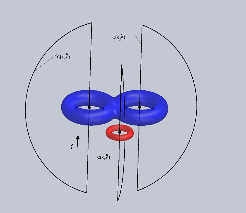
Figure 2: The curves $c(x,\hat{\mathbf{v}})$.

Suppose that $L(x,\hat{\mathbf{v}})\subset\Lambda$, and $L(x,\hat{\mathbf{v}})\cap B_{R}\neq\emptyset$. we denote by $c(x,\hat{\mathbf{v}})$ the curve consisting of the segment $L(x,\hat{\mathbf{v}})\cap\overline{B_{R}}$ and an arc on $\partial\overline{B_{R}}$ that connects the points $L(x,\hat{\mathbf{v}})\cap\partial\overline{B_{R}}$. We orient $c(x,\hat{\mathbf{v}})$ in such a way that the segment of straight line has the orientation of $\hat{\mathbf{v}}$. See Figure 2.

DEFINITION 4.3.

A line $L(x,\hat{\mathbf{v}})\subset\Lambda$ goes through holes of $K$ if $L(x,\hat{\mathbf{v}})\cap B_{R}\neq\emptyset$ and $[c(x,\hat{\mathbf{v}})]_{H_{1}(\Lambda;{\mathbb{R}})}\neq 0$. Otherwise we say that $L(x,\hat{\mathbf{v}})$ does not go through holes of $K$.

Note that this characterization of lines that go or do not go through holes of $K$ is independent of the $R$ that was used in the definition. This follows from the homotopic invariance of homology. See Theorem 11.2, page 59 of [13].

In an intuitive sense $[c(x,\hat{\mathbf{v}})]_{H_{1}(\Lambda;{\mathbb{R}})}=0$ means that $c(x,\hat{\mathbf{v}})$ is the boundary of a surface (actually of a chain) that is contained in $\Lambda$ and then it can not go through holes of $K$. Obviously, as $K\subset B_{R}$, if $L(x,\hat{\mathbf{v}})\cap B_{R}=\emptyset$ the line $L(x,\hat{\mathbf{v}})$ can not go through holes of $K$.

DEFINITION 4.4.

Two lines $L(x,\hat{\mathbf{v}}),L(y,\hat{\mathbf{w}})\subset\Lambda$ that go through holes of $K$ go through the same holes if $[c(x,\hat{\mathbf{v}})]_{H_{1}(\Lambda;{\mathbb{R}})}=\pm[c(y,\hat{\mathbf{w}})]_{H_{1}(\Lambda;{\mathbb{R}})}$. Furthermore, we say that the lines go through the holes in the same direction if $[c(x,\hat{\mathbf{v}})]_{H_{1}(\Lambda;{\mathbb{R}})}=[c(y,\hat{\mathbf{w}})]_{H_{1}(\Lambda;{\mathbb{R}})}$.

REMARK 4.5.

If $(x,\hat{\mathbf{v}})\in\Lambda\times{\mathbb{S}}^{2}$, there are neighborhoods $B_{x}\subset{\mathbb{R}}^{3},B_{\hat{\mathbf{v}}}\subset{\mathbb{S}}^{2}$ such that $(x,\hat{\mathbf{v}})\in B_{x}\times B_{\hat{\mathbf{v}}}$ and if $(y,\hat{\mathbf{w}})\in B_{x}\times B_{\hat{\mathbf{v}}}$ then, the following is true: if $L(x,\hat{\mathbf{v}})$ does not go true holes of $K$, then, also $L(y,\hat{\mathbf{w}})$ does not go through holes of $K$. If $L(x,\hat{\mathbf{v}})$ goes through holes of $K$, then, $L(y,\hat{\mathbf{w}})$ goes through the same holes and in the same direction. This follows from the homotopic invariance of homology, Theorem 11.2, page 59 of [13].

DEFINITION 4.6.

For any $\hat{\mathbf{v}}\in{\mathbb{S}}^{2}$ we denote by $\Lambda_{\hat{\mathbf{v}},\hbox{\rm out}}$ the set of points $x\in\Lambda_{\hat{\mathbf{v}}}$ such that $L(x,\hat{\mathbf{v}})$ does not go through holes of $K$. We call this set the region without holes of $\Lambda_{\hat{\mathbf{v}}}$. The holes of $\Lambda_{\hat{\mathbf{v}}}$ is the set $\Lambda_{\hat{\mathbf{v}},\hbox{\rm in}}:=\Lambda_{\hat{\mathbf{v}}}\setminus\Lambda_{\hat{\mathbf{v}},\hbox{\rm out}}$.

$\Box$

We define the following equivalence relation on $\Lambda_{\hat{\mathbf{v}},\hbox{\rm in}}$. We say that $xR_{\hat{\mathbf{v}}}y$ if and only if $L(x,\hat{\mathbf{v}})$ and $L(y,\hat{\mathbf{v}})$ go through the same holes and in the same direction. By $[x]$ we designate the classes of equivalence under $R_{\hat{\mathbf{v}}}$. We denote by $\left\{\Lambda_{\hat{\mathbf{v}},h}\right\}_{h\in\mathcal{I}}$ the partition of $\Lambda_{\hat{\mathbf{v}},\hbox{\rm in}}$ given by this equivalence relation. It is defined as follows.

$$\mathcal{I}:=\{[x]\}_{x\in\Lambda_{\hat{\mathbf{v}},\hbox{\rm in}}}.$$

Given $h\in\mathcal{I}$ there is $x\in\Lambda_{\hat{\mathbf{v}},\hbox{\rm in}}$ such that $h=[x]$. We denote,

$$\Lambda_{\hat{\mathbf{v}},h}:=\{y\in\Lambda_{\hat{\mathbf{v}},\hbox{\rm in}}:yR_{\hat{\mathbf{v}}}x\}.$$

Then,

$$\Lambda_{\hat{\mathbf{v}},\hbox{\rm in}}=\cup_{h\in\mathcal{I}}\Lambda_{\hat{\mathbf{v}},h},\,\,\,\,\Lambda_{\hat{\mathbf{v}},h_{1}}\cap\Lambda_{\hat{\mathbf{v}},h_{2}}=\emptyset,\,h_{1}\neq h_{2}.$$

We call $\Lambda_{\hat{\mathbf{v}},h}$ the subset of $\Lambda_{\hat{\mathbf{v}}}$ that goes through the holes $h$ of $K$ in the direction of $\hat{\mathbf{v}}$. Note that

$$\{\Lambda_{\hat{\mathbf{v}},h}\}_{h\in\mathcal{I}}\cup\{\Lambda_{\hat{\mathbf{v}},\hbox{\rm out}}\}$$ (4.7)

is an disjoint open cover of $\Lambda_{\hat{\mathbf{v}}}$.

We visualize the dynamics of the electrons that travel through the holes of $K$ in $\Lambda_{\hat{\mathbf{v}},h}$ as follows. For large negative times the incoming electron wave packet is in $\Lambda$, far away from $K$. As time increases the electron travels towards $K$ and it reaches the region where $K$ is located, let us say that it is inside $B_{R}$. As these times the electron has to be in $\Lambda_{\hat{\mathbf{v}},h}$ in order cross $B_{R}$ through the holes of $K$ in $\Lambda_{\hat{\mathbf{v}},h}$. After crossing the holes it travels again away from $K$ towards spatial infinity in $\Lambda$. This means that the classical trajectories have to be in the following domain,

$$\mathcal{C}_{h}:=\left[\Lambda\setminus\left(\overline{B_{R}}\cup P_{\hat{\mathbf{v}}}\right)\right]\cup\left(\overline{B_{R}}\cap\Lambda_{\hat{\mathbf{v}},h}\right),$$ (4.8)

where $P_{\hat{\mathbf{v}}}$ is the plane orthogonal to $\hat{\mathbf{v}}$ that passes through zero,

$$P_{\hat{\mathbf{v}}}:=\left\{x\in{\mathbb{R}}^{3}:x\cdot\hat{\mathbf{v}}=0\right\}.$$ (4.9)

Note that we take away from $\mathcal{C}_{h}$ the part of $P_{\hat{\mathbf{v}}}$ that does not intersects $\Lambda_{\mathbf{v},h}$ in order that the only way that the electron in $\mathcal{C}_{h}$ can classically cross the plane $P_{\hat{\mathbf{v}}}$ is through $\Lambda_{\hat{\mathbf{v}},h}$.

In a similar way, the classical trajectories of the electrons that do not cross any hole of $K$ have to be on the set

$$\mathcal{C}_{\rm out}:=\left(\Lambda\setminus\overline{B_{R}}\right)\cup\left(\overline{B_{R}}\cap\Lambda_{\hat{\mathbf{v}},\rm out}\right).$$ (4.10)

In Corollary 5.9 in the appendix we prove that that the first group of singular homology with coefficients in ${\mathbb{R}}$ of $\mathcal{C}_{h},H_{1}(\mathcal{C}_{h};{\mathbb{R}}),h\in\mathcal{I}$, and of $\mathcal{C}_{\rm out},H_{1}(\mathcal{C}_{\rm out};{\mathbb{R}})$ are trivial. We actually prove that the first de Rham cohomology class of $\mathcal{C}_{h}$ and of $\mathcal{C}_{\rm out}$ are trivial by explicitly constructing a function $\lambda$ such that $A=\nabla\lambda$ for any magnetic potential $A$ with ${\rm curl}\,A=0$, or in differential geometric language by constructively proving that any closed one form is exact. Then, the triviality of the the first group of singular homology with coefficients in ${\mathbb{R}}$ of $\mathcal{C}_{h}$ and of $\mathcal{C}_{\rm out}$ follows from de Rham’s theorem (Theorem 4.17 page 154 of [32]).

Let $x_{0}$ be a fixed point with $x_{0}\cdot\hat{\mathbf{v}}<-R$. We define,

$$\lambda_{h}(x):=\int_{C^{h}}\,A,\quad h\in\mathcal{I},\,\hbox{\rm where $C^{h}$ is any differentiable path from $x_{0}$ to $x$ in $\mathcal{C}_{h}$},$$ (4.11)

and,

$$\lambda_{\rm out}(x):=\int_{C^{{\rm out}}}\,A,\quad\hbox{\rm where $C^{\rm out}$ is any differentiable path from $x_{0}$ to $x$ in $\mathcal{C}_{\rm out}$}.$$ (4.12)

Since $H_{1}(\mathcal{C}_{h};{\mathbb{R}}),h\in\mathcal{I}$ and $H_{1}(\mathcal{C}_{\rm out};{\mathbb{R}})$ are trivial, $\lambda_{h},h\in\mathcal{I}$ and $\lambda_{\rm out}$ do not depend in the particular curve form $x_{0}$ to $x$ that we take, respectively, in $\mathcal{C}_{h},h\in\mathcal{I}$ and $\mathcal{C}_{\rm out}$. Furthermore, they are differentiable and $\nabla\lambda_{h}(x)=A(x),x\in\mathcal{C}_{h},h\in\mathcal{I}$ and $\nabla\lambda_{\rm out}(x)=A(x),x\in\mathcal{C}_{\rm out}$.

Before we prove the validity of the Aharonov-Bohm Ansatz we prepare some simple results on the free evolution that we need. Below we denote by $\widetilde{O}$ the complement of any set $O\subset{\mathbb{R}}^{3}$.

LEMMA 4.7.

We denote,

$$C_{-,h}:=\{x\in\Lambda\setminus\overline{B_{R}}:x\cdot\hat{\mathbf{v}}<0\}\cup\Lambda_{\hat{\mathbf{v}},h},h\in\mathcal{I},\quad C_{-,\rm out}:=\{x\in\Lambda\setminus\overline{B_{R}}:x\cdot\hat{\mathbf{v}}<0\}\cup\Lambda_{\hat{\mathbf{v}},\rm out}.$$ (4.13)

Then, for any $l=0,1,\cdots$ and any compact set $\Lambda_{0}\subset\Lambda_{\hat{\mathbf{v}},h},h\in\mathcal{I}$ there is a constant $C_{l}$ such that $\forall Z\geq 0,\forall z\in(-\infty,Z]$, and for all $\varphi\in\mathcal{H}_{2}({\mathbb{R}}^{3})$ with support in $\Lambda_{0}$,

$$\left\|\chi_{\displaystyle\widetilde{C_{-,h}}}\,e^{-i\frac{z}{v}H_{0}}\,\varphi_{\mathbf{v}}\right\|_{L^{2}({\mathbb{R}}^{3})}\leq C_{l}\,\left((1+Z)^{-l}+\frac{1+Z}{v}\right)\|\varphi\|_{\mathcal{H}_{2}({\mathbb{R}}^{3})}.$$ (4.14)

Furthermore, for any $l=0,1,\cdots$ and any compact set $\Lambda_{0}\subset\Lambda_{\hat{\mathbf{v}},\rm out}$ there is a constant $C_{l}$ such that $\forall Z\geq 0,\forall z\in(-\infty,Z]$, and for all $\varphi\in\mathcal{H}_{2}({\mathbb{R}}^{3})$ with support in $\Lambda_{0}$,

$$\left\|\chi_{\displaystyle\widetilde{C_{-,\rm out}}}\,e^{-i\frac{z}{v}H_{0}}\,\varphi_{\mathbf{v}}\right\|_{L^{2}({\mathbb{R}}^{3})}\leq C_{l}\,\left((1+Z)^{-l}+\frac{1+Z}{v}\right)\|\varphi\|_{\mathcal{H}_{2}({\mathbb{R}}^{3})}.$$ (4.15)

Proof: We give the proof of (4.14). Equation (4.15) follows in the same way.

1. Suppose that $z\leq\,{\rm min}\,(-\frac{4}{3}R,-Z)$. By (3.16) it is enough to prove (4.14) for $\tilde{\varphi}$. The estimate follows from (3.9) and Lemma 3.2 observing that $\chi_{\displaystyle\widetilde{C_{-,h}}}(x)=\chi_{\displaystyle\widetilde{C_{-,h}}}(x)F(|x-z\hat{\mathbf{v}}|>|z|/4)$.

2. Suppose that $z\in[-Z,Z]$. Since, $\chi_{\displaystyle\widetilde{C_{-,h}}}\,e^{\displaystyle-iz\mathbf{p}\cdot\hat{\mathbf{v}}}\,\varphi=0$, it follows from (3.8) that,

   $$\begin{array}[]{l}\left\|\chi_{\displaystyle\widetilde{C_{-,h}}}\,e^{-i\frac{z}{v}H_{0}}\,\varphi_{\mathbf{v}}\right\|_{L^{2}({\mathbb{R}}^{3})}=\left\|\chi_{\displaystyle\widetilde{C_{-,h}}}\,\left[e^{-izH_{1}}-e^{\displaystyle-iz\mathbf{p}\cdot\hat{\mathbf{v}}}e^{\displaystyle-izmv/2}\right]\,\varphi\right\|_{L^{2}({\mathbb{R}}^{3})}\leq\\ \\ C\frac{Z}{v}\,\|\varphi\|_{\mathcal{H}_{2}({\mathbb{R}}^{3})}.\end{array}$$ (4.16)

3. If $Z\leq\frac{4}{3}R$ it remains to consider $z\in[-\frac{4}{3}R,-Z]$. In this case we just say that,

   $$\left\|\chi_{\displaystyle\widetilde{C_{-,h}}}\,e^{-i\frac{z}{v}H_{0}}\,\varphi_{\mathbf{v}}\right\|_{L^{2}({\mathbb{R}}^{3})}\leq\|\varphi\|_{L^{2}({\mathbb{R}}^{3})}\leq C_{l}(1+Z)^{-l}\,\|\varphi\|_{L^{2}({\mathbb{R}}^{3})}.$$ (4.17)

LEMMA 4.8.

We denote,

$$C_{+}^{0}:=\{x\in\Lambda\setminus\overline{B_{R}}:x\cdot\hat{\mathbf{v}}>0\}.$$ (4.18)

Then, for any $l=0,1,\cdots$ there is a constant $C_{l}$ such that $\forall Z\geq 0,\forall z\geq Z$, and for all $\varphi\in\mathcal{H}_{2}({\mathbb{R}}^{3})$,

$$\left\|\chi_{\displaystyle\widetilde{C_{+}^{0}}}\,e^{-i\frac{z}{v}H_{0}}\,\varphi_{\mathbf{v}}\right\|_{L^{2}({\mathbb{R}}^{3})}\leq C_{l}\,\left((1+Z)^{-l}+\frac{1}{v}\right)\|\varphi\|_{\mathcal{H}_{2}({\mathbb{R}}^{3})}.$$ (4.19)

Proof: If $Z\geq\,\frac{4}{3}R$ we prove (4.19) as in item 1 of the proof of Lemma 4.7 observing that $\chi_{\displaystyle\widetilde{C_{+}}}(x)=\chi_{\displaystyle\widetilde{C_{+}}}(x)F(|x-z\hat{\mathbf{v}}|>|z|/4)$. If $Z\leq\frac{4}{3}R$ it remains to consider $z\in[Z,\frac{4}{3}R]$ but in this case (4.19) follows as in item 3 of the proof of Lemma 4.7.

COROLLARY 4.9.

For any $l=0,1,\cdots$ and any compact set $\Lambda_{0}\subset\Lambda_{\hat{\mathbf{v}},h},h\in\mathcal{I}$ there is a constant $C_{l}$ such that $\forall Z\geq 0,\forall z\in{\mathbb{R}}$, and for all $\varphi\in\mathcal{H}_{2}({\mathbb{R}}^{3})$ with support in $\Lambda_{0}$,

$$\left\|\chi_{\displaystyle\widetilde{\mathcal{C}_{h}}}\,e^{-i\frac{z}{v}H_{0}}\,\varphi_{\mathbf{v}}\right\|_{L^{2}({\mathbb{R}}^{3})}\leq C_{l}\,\left((1+Z)^{-l}+\frac{1+Z}{v}\right)\|\varphi\|_{\mathcal{H}_{2}({\mathbb{R}}^{3})}.$$ (4.20)

Furthermore, for any $l=0,1,\cdots$ and any compact set $\Lambda_{0}\subset\Lambda_{\hat{\mathbf{v}},\rm out}$ there is a constant $C_{l}$ such that $\forall Z\geq 0,\forall z\in{\mathbb{R}}$, and for all $\varphi\in\mathcal{H}_{2}({\mathbb{R}}^{3})$ with support in $\Lambda_{0}$,

$$\left\|\chi_{\displaystyle\widetilde{\mathcal{C}_{\rm out}}}\,e^{-i\frac{z}{v}H_{0}}\,\varphi_{\mathbf{v}}\right\|_{L^{2}({\mathbb{R}}^{3})}\leq C_{l}\,\left((1+Z)^{-l}+\frac{1+Z}{v}\right)\|\varphi\|_{\mathcal{H}_{2}({\mathbb{R}}^{3})}.$$ (4.21)

Proof : Note that since

$$\left(\Lambda\setminus\overline{B_{R}}\right)\cap\Lambda_{\hat{\mathbf{v}},h}\subset\left[\Lambda\setminus\left(\overline{B_{R}}\cup P_{\hat{\mathbf{v}}}\right)\right],\quad h\in\mathcal{I},$$

we have that,

$$C_{-,h}\subset\mathcal{C}_{h},h\in\mathcal{I}.$$

Moreover,

$$C_{-,\rm out}\subset\mathcal{C}_{\rm out},$$

and,

$$C_{+}^{0}\subset\mathcal{C}_{h}\,\cap\,\mathcal{C}_{\rm out}.$$

Hence, the corollary follows from Lemma 4.7 when $z\leq Z$ and from Lemma 4.8 when $z\geq Z$.

DEFINITION 4.10.

We designate by $\mathcal{A}_{\Phi,2\pi}(0)$ the set of all potentials $A\in\mathcal{A}_{\Phi,2\pi}(B)$ that satisfy,

$${\rm curl}\,A=B=0.$$

REMARK 4.11.

For any $A\in\mathcal{A}_{\Phi,2\pi}(0)\cap C^{l}(\overline{\Lambda},{\mathbb{R}}^{3}),l=1,2,\cdots$ there is a $\tilde{A}\in\mathcal{A}_{\Phi,2\pi}(0)\cap C^{l}(\overline{\Lambda},{\mathbb{R}}^{3})$ with the same flux as $A$ and with support$\tilde{A}\subset B_{R}$. To prove this statement we take any $x_{0}\in\Lambda\setminus B_{R}$ and let $\varepsilon>0$ be so small that $K\subset B_{R-\varepsilon}$. We define,

$$\overline{\lambda}(x):=\int_{C(x_{o},x)}A,\quad{\rm for}\,x\in\Lambda\setminus B_{R-\varepsilon},$$

where $C(x_{0},x)$ is any differentiable path from $x_{0}$ to $x$ contained in $\Lambda\setminus B_{R-\varepsilon}$. Then, $\overline{\lambda}\in C^{l}(\overline{\Lambda}\setminus B_{R-\varepsilon})$. We denote by $\lambda$ any extension of $\overline{\lambda}$ to ${\mathbb{R}}^{3}$ such that $\lambda\in C^{l}({\mathbb{R}}^{3})$ [31]. We define,

$$\tilde{A}(x):=A(x)-\nabla\lambda(x),\quad x\in\overline{\Lambda}.$$

Then, $\tilde{A}\in\mathcal{A}_{\Phi,2\pi}(0)\cap C^{l}(\overline{\Lambda},{\mathbb{R}}^{3}),l=1,2,\cdots$, the flux of $\tilde{A}$ is the same as the one of $A$ and support$\tilde{A}\subset B_{R}$. Note that if $B=0$ the Coulomb potential $A_{C}\in C^{\infty}(\overline{\Lambda},{\mathbb{R}}^{3})$ (see Theorem 3.7 of [4]). Doing the gauge transformation above we see that for every $l=1,2,\cdots$ there is a potential in $\mathcal{A}_{\Phi,2\pi}(0)\cap C^{l}(\overline{\Lambda},{\mathbb{R}}^{3})$ with compact support in $B_{R}$.

By Remark 4.11 we can use the freedom of taking a gauge transformation to assume that $A\in\mathcal{A}_{\Phi,2\pi}(0)\cap C^{1}(\overline{\Lambda},{\mathbb{R}}^{3})$ and that support$A\subset B_{R}$, what we do from now on.

THEOREM 4.12.

For any $l=0,1,\cdots$ and any compact set $\Lambda_{0}\subset\Lambda_{\hat{\mathbf{v}},h},h\in\mathcal{I}$ there is a constant $C_{l}$ such that $\forall Z\geq 0,\forall z\in{\mathbb{R}}$, and for all $\varphi\in\mathcal{H}_{2}({\mathbb{R}}^{3})$ with support in $\Lambda_{0}$,

$$\left\|e^{\displaystyle-i\frac{z}{v}H(A,V)}\,W_{-}(A,V)\,\varphi_{\mathbf{v}}-e^{i\lambda_{h}}\,\chi_{\displaystyle\mathcal{C}_{h}}\,e^{-i\frac{z}{v}H_{0}}\,\varphi_{\mathbf{v}}\right\|_{L^{2}({\mathbb{R}}^{3})}\leq C_{l}\,\left((1+Z)^{-l}+\frac{1+Z}{v}\right)\|\varphi\|_{\mathcal{H}_{2}({\mathbb{R}}^{3})}.$$ (4.22)

Furthermore, for any $l=0,1,\cdots$ and any compact set $\Lambda_{0}\subset\Lambda_{\hat{\mathbf{v}},\rm out}$ there is a constant $C_{l}$ such that $\forall Z\geq 0,\forall z\in{\mathbb{R}}$, and for all $\varphi\in\mathcal{H}_{2}({\mathbb{R}}^{3})$ with support in $\Lambda_{0}$,

$$\left\|e^{\displaystyle-i\frac{z}{v}H(A,V)}\,W_{-}(A,V)\,\varphi_{\mathbf{v}}-e^{i\lambda_{\rm out}}\,\chi_{\displaystyle\mathcal{C}_{\rm out}}\,e^{-i\frac{z}{v}H_{0}}\,\varphi_{\mathbf{v}}\right\|_{L^{2}({\mathbb{R}}^{3})}\leq C_{l}\,\left((1+Z)^{-l}+\frac{1+Z}{v}\right)\|\varphi\|_{\mathcal{H}_{2}({\mathbb{R}}^{3})}.$$ (4.23)

Proof: We first consider the case $z\leq Z$. In this case the theorem follows from Lemmata 4.7, 4.8, Corollary 4.9, and (3.59) observing that that since support $A\subset B_{R}$ ,

$$-L_{A,\hat{\mathbf{v}}}(-\infty)=\lambda_{h}(x),\quad x\in C_{-,h},h\in\mathcal{I},\quad-L_{A,\hat{\mathbf{v}}}(-\infty)=\lambda_{\rm out}(x),\quad x\in C_{-,\rm out}.$$

For $z\geq Z$ we use (3.61), Lemma 4.8 and Corollary 4.9. For this purpose note that,

$$\int_{-\infty}^{\infty}\,A(x+\tau\hat{\mathbf{v}})\cdot\hat{\mathbf{v}}\,d\tau=\int_{c(x,\hat{\mathbf{v}})}\,A,\quad\,{\rm for}\,x\in\Lambda_{\hat{\mathbf{v}},h},h\in\mathcal{I},\int_{-\infty}^{\infty}\,A(x+\tau\hat{\mathbf{v}})\cdot\hat{\mathbf{v}}\,d\tau=0,\,{\rm for}\,x\in\Lambda_{\rm out}.$$

Moreover, recall that (see Definition 7.10 of [4])

$$F_{h}:=\int_{c(x,\hat{\mathbf{v}})}\,A,\quad x\in\Lambda_{\hat{\mathbf{v}},h},h\in\mathcal{I},$$

and that $F_{h}$ is constant for all $x\in\Lambda_{\hat{\mathbf{v}},h}$. $F_{h}$ is the magnetic flux over any surface (or a chain) in ${\mathbb{R}}^{3}$ whose boundary is $c(x,\hat{\mathbf{v}})$. In other words, it is the flux associated to the holes of $K$ in $\Lambda_{\hat{\mathbf{v}},h}$ . Furthermore, we have that,

$$F_{h}=\lambda_{h}(x),\quad x\in C_{+}^{0},$$ (4.24)

what completes the proof for $z\geq Z,h\in\mathcal{I}$. For the case $\Lambda_{\hat{\mathbf{v}},\rm out}$ and $z\geq Z$ we observe that,

$$\lambda_{\rm out}(x)=0,\quad{\rm for}\,x\in C_{+}^{0}.$$ (4.25)

We now state our main results on the validity of the Aharonov-Bohm Ansatz.

THEOREM 4.13.

For any $1>\delta>0$ and any compact set $\Lambda_{0}\subset\Lambda_{\hat{\mathbf{v}},h},h\in\mathcal{I}$ there is a constant $C_{\delta}$ such that $\forall t\in{\mathbb{R}}$ and for all $\varphi\in\mathcal{H}_{2}({\mathbb{R}}^{3})$ with support in $\Lambda_{0}$,

$$\left\|e^{\displaystyle-itH(A,V)}\,W_{-}(A,V)\,\varphi_{\mathbf{v}}-e^{i\lambda_{h}}\,\chi_{\displaystyle\mathcal{C}_{h}}\,e^{-itH_{0}}\,\varphi_{\mathbf{v}}\right\|_{L^{2}({\mathbb{R}}^{3})}\leq\frac{C_{\delta}}{v^{1-\delta}}\|\varphi\|_{\mathcal{H}_{2}({\mathbb{R}}^{3})}.$$ (4.26)

Furthermore, for any $1>\delta>0$ and any compact set $\Lambda_{0}\subset\Lambda_{\hat{\mathbf{v}},\rm out}$ there is a constant $C_{\delta}$ such that $\forall t\in{\mathbb{R}}$ and for all $\varphi\in\mathcal{H}_{2}({\mathbb{R}}^{3})$ with support in $\Lambda_{0}$,

$$\left\|e^{\displaystyle-itH(A,V)}\,W_{-}(A,V)\,\varphi_{\mathbf{v}}-e^{i\lambda_{\rm out}}\chi_{\displaystyle\mathcal{C}_{\rm out}}\,e^{-itH_{0}}\,\varphi_{\mathbf{v}}\right\|_{L^{2}({\mathbb{R}}^{3})}\leq\frac{C_{\delta}}{v^{1-\delta}}\|\varphi\|_{\mathcal{H}_{2}({\mathbb{R}}^{3})}.$$ (4.27)

Proof: we take in Theorem 4.12, $Z=v^{1/(1+l)}$ and $t=z/v$ . Then, for $v>1$, $\frac{1}{v}(1+Z)\leq 2\frac{1}{v^{1-1/(1+l)}}$ and $(1+Z)^{-l}\leq\frac{1}{v^{1-1/(1+l)}}$. The theorem follows taking $\frac{1}{1+l}\leq\delta$.

$\Box$

Let us take any $\varphi_{0}\in\mathcal{H}_{2}({\mathbb{R}}^{3})$ with compact support in $\Lambda_{\hat{\mathbf{v}}}$. Then, since (4.7) is a disjoint open cover of $\Lambda_{\hat{\mathbf{v}}}$

$$\varphi_{0}=\sum_{h\in\mathcal{I}}\,\varphi_{h}+\varphi_{\rm out},$$ (4.28)

where $\varphi_{h},\varphi_{\rm out}\in\mathcal{H}_{2}({\mathbb{R}}^{3}),\varphi_{h}$ has compact support in $\Lambda_{\hat{\mathbf{v}},h},h\in\mathcal{I},$ and $\varphi_{\rm out}$ has compact support in $\Lambda_{\hat{\mathbf{v}},\rm out}$. The sum is finite because $\varphi_{0}$ has compact support. We denote,

$$\varphi_{\mathbf{v}}:=e^{im\mathbf{v}\cdot x}\,\varphi_{0},\,\varphi_{\mathbf{v},h}:=e^{im\mathbf{v}\cdot x}\,\varphi_{h},h\in\mathcal{I},\varphi_{\mathbf{v},\rm out}:=e^{im\mathbf{v}\cdot x}\,\varphi_{\rm out}.$$ (4.29)

We define,

$$\psi_{AB,\mathbf{v},h}:=\chi_{\mathcal{C}_{h}}\,e^{i\lambda_{h}}\,e^{-itH_{0}}\,\varphi_{\mathbf{v},h},h\in\mathcal{I},\quad\psi_{AB,\mathbf{v},\rm out}:=\chi_{\mathcal{C}_{\rm out}}\,e^{i\lambda_{\rm out}}\,e^{-itH_{0}}\,\varphi_{\mathbf{v},\rm out},$$ (4.30)

$$\psi_{AB,\mathbf{v}}:=\sum_{h\in\mathcal{I}}\,\psi_{AB,\mathbf{v},h}+\psi_{AB,\mathbf{v},\rm out}.$$ (4.31)

Equation (4.31) gives the Aharonov-Bohm Ansatz in the domain $\cup_{h\in\mathcal{I}}\mathcal{C}_{h}\cup\mathcal{C}_{\rm out}$ that has non-trivial first group of singular homology as the sum of the Aharonov-Bohm Ansätze in each of the components, $\mathcal{C}_{h},h\in\mathcal{I},\mathcal{C}_{\rm out}$ that have trivial first group of singular homology. As we already mentioned, for the Ansatz of Aharonov-Bohm to be valid, it is necessary that the electron does not hit the magnet. Otherwise, the electron will be reflected and the Ansatz cannot be an approximate solution because it consists of the free evolution multiplied by a phase in configuration space. Hence, the wave function that represents such an electron has to have its support approximately contained for all times in the domain $\cup_{h\in\mathcal{I}}\mathcal{C}_{h}\cup\mathcal{C}_{\rm out}$. In the next theorem we prove that the Ansatz of Aharonov-Bohm is actually valid on the biggest domain where it can be valid, $\cup_{h\in\mathcal{I}}\mathcal{C}_{h}\cup\mathcal{C}_{\rm out}$, and, in this way, we provide an approximate solution for all times for every electron that does not hit the magnet.

THEOREM 4.14.

The Validity of the Aharonov-Bohm Ansatz.

For any $1>\delta>0$ and any compact set $\Lambda_{0}\subset\Lambda_{\hat{\mathbf{v}}}$ there is a constant $C_{\delta}$ such that $\forall t\in{\mathbb{R}}$ and for all $\varphi\in\mathcal{H}_{2}({\mathbb{R}}^{3})$ with support in $\Lambda_{0}$ the solution to the Schrödinger equation $e^{\displaystyle-itH(A,V)}\,W_{-}(A,V)\,\varphi_{\mathbf{v}}$ that behaves as $e^{-itH_{0}}\,\varphi_{\mathbf{v}}$ as $t\rightarrow-\infty$ is given at time $t$ by the Aharonov-Bohm Ansatz, $\psi_{AB,\mathbf{v}}$, up to the following error,

$$\left\|e^{\displaystyle-itH(A,V)}\,W_{-}(A,V)\,\varphi_{\mathbf{v}}-\psi_{AB,\mathbf{v}}\right\|_{L^{2}({\mathbb{R}}^{3})}\leq\frac{C_{\delta}}{v^{1-\delta}}\|\varphi\|_{\mathcal{H}_{2}({\mathbb{R}}^{3})}.$$ (4.32)

Proof: The theorem follows from Theorem 4.13 and equations (4.28 to 4.31).

$\Box$

Note that by (4.24, 4.25) behind the magnet in $C^{0}_{+}$,

$$\psi_{AB,\mathbf{v},h}:=\chi_{\mathcal{C}_{h}}\,e^{iF_{h}}\,e^{-itH_{0}}\,\varphi_{\mathbf{v},h},h\in\mathcal{I},\quad x\in C^{0}_{+},$$ (4.33)

and that,

$$\psi_{AB,\mathbf{v},\rm out}:=\chi_{\mathcal{C}_{\rm out}}\,e^{-itH_{0}}\,\varphi_{\mathbf{v},\rm out},\quad\quad x\in C^{0}_{+}.$$ (4.34)

As mentioned in the introduction the phase shifts $e^{iF_{h}}$ were measured in the experiments of Tonomura et al. [20, 28, 29] and, furthermore, since the Aharonov-Bohm Ansatz is free evolution, up to a phase, the electron is not accelerated, what explains the results of the experiment of Caprez et al. [8]. Hence, Theorem 4.14 rigorously proves that quantum mechanics predicts the results of the experiments of Tonomura et al. and of Caprez et al..

5 Appendix

In this appendix we prove that the first group of singular homology with coefficients in ${\mathbb{R}}$ of $\mathcal{C}_{h}$ and of $\mathcal{C}_{\rm out}$ are trivial. The sets $\mathcal{C}_{h}$ and $\mathcal{C}_{\rm out}$ are defined, respectively, in (4.8) and (4.10). We denote

$$C_{+}:=\{x\in{\mathbb{R}}^{3}\setminus B_{R}:x\cdot\hat{\mathbf{v}}>0\},\quad C_{-}:=\{x\in{\mathbb{R}}^{3}\setminus B_{R}:x\cdot\hat{\mathbf{v}}<0\},$$ (5.1)

and by $C^{0}_{\pm}$ the interior of $C_{\pm}$. Recall that $P_{\hat{\mathbf{v}}}$ is defined in (4.9). Then,

$$\mathcal{C}_{h}=C^{0}_{-}\cup C^{0}_{+}\cup(\overline{B_{R}}\cap\Lambda_{\hat{\mathbf{v}},h}),$$ (5.2)

$$\mathcal{C}_{\rm out}=C^{0}_{-}\cup C^{0}_{+}\cup(\overline{B}_{R}\cap\Lambda_{\hat{\mathbf{v}},\rm out})\cup(P_{\hat{\mathbf{v}}}\setminus\overline{B}_{R}).$$ (5.3)

We first prepare several results that we need. Below we denote by $A$ any continuously differentiable vector field defined, respectively, in $\mathcal{C}_{h},h\in\mathcal{I}$, and in $\mathcal{C}_{\rm out}$, with ${\rm curl}\,A=0$.

Let $x_{0}$ be a fixed point with $x_{0}<-R$. For any $x\in B_{R}$ we denote, respectively by $x_{\rm in},x_{\rm out}$ the intersection of the line $\{x+\tau\hat{\mathbf{v}},\tau\in{\mathbb{R}}\}$ with $\partial B_{R}$ such that $x_{\rm in}\cdot\hat{\mathbf{v}}<0,x_{\rm out}\cdot\hat{\mathbf{v}}>0$. For any $h\in\mathcal{I}$ let $x^{h}$ be a fixed point in $\Lambda_{\hat{\mathbf{v}},h}\cap B_{R}$ and let $x^{\rm out}$ be a fixed point in $\Lambda_{\hat{\mathbf{v}},\rm out}\cap B_{R}$.

REMARK 5.1.

For every $x\in C_{-}$ we denote by $C_{-}^{x}$ any differentiable path in $C_{-}$ that goes from $x_{0}$ to $x$ and we define,

$$\lambda_{-}(x):=\int_{C_{-}^{x}}\,A.$$ (5.4)

Since $C_{-}$ is simply connected the line integral in (5.4) does not depend on the particular curve $C_{-}^{x}$ that we choose. Then, for $x\in C_{-}^{0},\,\lambda_{-}(x)$ is differentiable and $\nabla\lambda_{-}(x)=A(x)$.

REMARK 5.2.

For every $x\in B_{R}\cap\Lambda_{\hat{\mathbf{v}}}$ we denote by $C^{x}_{0}$ the differentiable path consisting of a path $C_{-}^{x_{\rm in}}$ followed by the segment $[x_{\rm in},x]$ and we define for every $x\in B_{R}\cap\Lambda_{\hat{\mathbf{v}}}$,

$$\lambda_{0}(x):=\int_{C^{x}_{0}}\,A.$$ (5.5)

By Remark 5.1 the line integral in (5.5) does not depend on the particular curve $C_{-}^{x_{\rm in}}$ that we choose. Then, for $x\in B_{R}\cap\Lambda_{\hat{\mathbf{v}}}$ , $\lambda_{0}(x)$ is differentiable and $\nabla\lambda_{0}(x)=A(x)$. To prove this statement we observe that for each $x\in B_{R}\cap\Lambda_{\hat{\mathbf{v}}}$ there is $\varepsilon>0$ such that $B_{\varepsilon}(x)\subset B_{R}\cap\Lambda_{\hat{\mathbf{v}}}$. The set $C_{s}:=\{C_{-}\cup(B_{\varepsilon}(x)+{\mathbb{R}}\hat{\mathbf{v}})\}$ is simply connected and, furthermore, $\lambda_{0}(x)=\int_{C}\,A$ where $C$ is any differentiable path contained in $C_{s}$ that goes from $x_{0}$ to $x$.

REMARK 5.3.

For every $x\in C_{+}$ and any $h\in\mathcal{I}$ we denote by $C_{h,+}^{x}$ a differentiable path consisting of any curve $\displaystyle C_{-}^{x^{h}_{\rm in}}$ followed from the segment $[x^{h}_{\rm in},x^{h}_{\rm out}]$ and of a differentiable path $C_{+}^{x^{h}_{\rm out},x}$ in $C_{+}$. The differentiable path $C_{\rm out,+}^{x}$ is defined in the same way, but replacing $x^{h}$ by $x^{\rm out}$. We define,

$$\lambda_{+}^{h}(x):=\int_{C_{h,+}^{x}}\,A,\quad x\in C_{+},h\in\mathcal{I},$$ (5.6)

and

$$\lambda_{+}^{\rm out}(x):=\int_{C_{\rm out,+}^{x}}\,A,\quad x\in C_{+}.$$ (5.7)

Since $C_{\pm}$ are simple connected $\lambda_{+}^{h}$ does not depends of the particular paths $\displaystyle C_{-}^{x^{h}_{\rm in}},C_{+}^{x^{h}_{\rm out},x}$ that we choose and, $\lambda_{+}^{\rm out}$ does not depends of the particular paths $\displaystyle C_{-}^{x^{\rm out}_{\rm in}},C_{+}^{x^{\rm out}_{\rm out},x}$ that we choose . It follows that $\lambda_{+}^{h}$ and $\lambda_{+}^{\rm out}$ are continuously differentiable in $C_{+}^{0}$ and that $\nabla\lambda_{+}^{h}(x)=A(x)$, $\nabla\lambda_{+}^{\rm out}(x)=A(x)$.

REMARK 5.4.

$\lambda_{+}^{h},h\in\mathcal{I}$ does not depend of the particular $x^{h}\in\Lambda_{\hat{\mathbf{v}},h}$ that we choose. To prove this statement let us take any $y\in\Lambda_{\hat{\mathbf{v}},h}\cap B_{R}$ and let the differentiable path $C_{y,+}^{x}$ be defined as $C_{h,+}^{x}$ but with $y$ instead of $x^{h}$. Let $\gamma$ be any differentiable path from $x$ to $x_{0}$ contained in $\Lambda\setminus B_{R}$. Let $C$ be a the closed oriented differentiable path consisting of $C_{h,+}^{x}$, from $x_{0}$ to $x$, followed from $\gamma$. $C_{y}$ is defined in the same way, but with $C_{y,+}^{x}$ instead of $C_{h,+}^{x}$. Let $D$ be an arc on $\partial B_{R}$ from $x_{\rm in}^{h}$ to $x_{\rm out}^{h}$ and let $G$ be a differentiable path consisting of $\displaystyle C_{-}^{x^{h}_{\rm in}}$ followed of $D,C_{+}^{x^{h}_{\rm out},x}$ and $\gamma$. Since ${\mathbb{R}}^{3}\setminus B_{R}$ is simply connected we have that,

$$\int_{G}\,A=0,$$

and then,

$$\int_{C}\,A=\int_{c(x^{h}_{\rm in},\hat{\mathbf{v}})}\,A.$$

We prove in the same way that,

$$\int_{C_{y}}\,A=\int_{c(y_{\rm in},\hat{\mathbf{v}})}\,A.$$

Furthermore, since $x^{h},y\in\Lambda_{\hat{\mathbf{v}},h}$, we have that $[c(x^{h}_{\rm in},\hat{\mathbf{v}})]_{H_{1}(\Lambda;{\mathbb{R}})}=[c(y_{\rm in},\hat{\mathbf{v}})]_{H_{1}(\Lambda;{\mathbb{R}})}$, and then, by Stoke’s theorem,

$$\int_{c(x^{h}_{\rm in},\hat{\mathbf{v}})}\,A=\int_{c(y_{\rm in},\hat{\mathbf{v}})}\,A,$$

what proves that,

$$\int_{C}\,A=\int_{C_{y}}\,A,$$

and then,

$$\lambda_{+}^{h}(x):=\int_{C_{h,+}^{x}}\,A=\int_{C_{y,+}^{x}}\,A.$$

REMARK 5.5.

$\lambda_{+}^{\rm out}$ does not depend of the particular $x^{\rm out}\in\Lambda_{\hat{\mathbf{v}},\rm out}$ that we choose. This is proven as in Remark 5.4 replacing $x^{h}$ by $x^{\rm out}$. Furthermore, as in this case $[c(x^{\rm out}_{\rm in},\hat{\mathbf{v}})]_{H_{1}(\Lambda;{\mathbb{R}})}=0$,

$$\int_{C}\,A=0,$$

and then,

$$\lambda_{+}^{\rm out}(x)=\int_{\gamma}\,A,$$ (5.8)

where $\gamma$ is any differentiable path from $x_{0}$ to $x$ contained in $\Lambda\setminus B_{R}$.

DEFINITION 5.6.

For all $h\in\mathcal{I}$ we define $\lambda^{h}:\mathcal{C}_{h}\rightarrow{\mathbb{R}}$ as follows,

$$\lambda^{h}(x):=\left\{\begin{array}[]{l}\lambda_{-}(x),\quad\hbox{\rm if}\,\,x\in C_{-},\\ \\ \lambda_{0}(x),\quad\hbox{\rm if}\,\,x\in\Lambda_{\hat{\mathbf{v}},h}\cap B_{R},\\ \\ \lambda_{+}^{h}(x),\quad\hbox{\rm if}\,\,x\in C_{+}.\end{array}\right.$$ (5.9)

Furthermore, we define $\lambda^{\rm out}:\mathcal{C}_{\rm out}\rightarrow{\mathbb{R}}$ as,

$$\lambda^{\rm out}(x):=\left\{\begin{array}[]{l}\lambda_{-}(x),\quad\hbox{\rm if}\,\,x\in C_{-},\\ \\ \lambda_{0}(x),\quad\hbox{\rm if}\,\,x\in\Lambda_{\hat{\mathbf{v}},\rm out}\cap B_{R},\\ \\ \lambda_{+}^{\rm out}(x),\quad\hbox{\rm if}\,x\in C_{+},\\ \\ \int_{\gamma}\,A,\hbox{\rm if \, $x\in P_{\hat{\mathbf{v}}}\setminus B_{R}$, where $\gamma$ is any differentiable path from $x_{0}$ to $x$ contained in $\Lambda\setminus B_{R}$ }.\end{array}\right.$$ (5.10)

LEMMA 5.7.

The functions $\lambda^{h},h\in\mathcal{I}$ and $\lambda^{\rm out}$ are continuously differentiable and $\nabla\lambda^{h}(x)=A(x),x\in\mathcal{C}_{h},h\in\mathcal{I}$ and $\nabla\lambda^{\rm out}(x)=A(x),x\in\mathcal{C}^{\rm out}$.

Proof: We first consider $\lambda^{h},h\in\mathcal{I}$. By Remarks 5.1, 5.2 and 5.3 $\lambda^{h}(x)$ is continuously differentiable and $\nabla\lambda^{h}(x)=A(x)$ for $x\in C_{-}^{0}\cup C_{+}^{0}\cup\Lambda_{\hat{\mathbf{v}},h}\cap B_{R}$. If follows from (5.2) that it only remains to prove the result for $x\in\Lambda_{\hat{\mathbf{v}},h}\cap\partial B_{R}$. Let $\varepsilon>0$ be such that, $B_{\varepsilon}(x)\subset\Lambda_{\hat{\mathbf{v}},h}$ (see Remark 4.5). The set

$$C_{p,h}:=\{C_{-}^{0}\cup(B_{\varepsilon}(x)+{\mathbb{R}}\hat{\mathbf{v}})\cup C_{+}^{0}\}$$

is simply connected and by Remark 5.4

$$\lambda^{h}(y)=\int_{C}\,A,\quad y\in C_{p,h},$$

where $C$ is any differentiable path from $x_{0}$ to y that is contained in $C_{p,h}$. It follows that $\lambda^{h}(x)$ is differentiable for $x\in\Lambda_{\hat{\mathbf{v}},h}\cap\partial B_{R}$ and that $\nabla\lambda^{h}(x)=A(x)$.

Let us now consider $\lambda^{\rm out}$. By Remarks 5.1, 5.2 and 5.3 the lemma holds for $x\in C_{-}^{0}\cup C_{+}^{0}\cup\left(\Lambda_{\hat{\mathbf{v}},\rm out}\cap B_{R}\right)$. Furthermore, by the definition of $\lambda^{\rm out}$ and (5.8) it also holds for $x\in P_{\hat{\mathbf{v}}}\setminus\overline{B_{R}}$. By (5.3) it only remains to consider the case of $x\in\partial B_{R}\cap\Lambda_{\hat{\mathbf{v}},\rm out}$. Take $\varepsilon>0$ such that $K\subset B_{R-\varepsilon}$. Then, since ${\mathbb{R}}^{3}\setminus\overline{B_{R-\varepsilon}}$ is a simply connected set where ${\rm curl}A=0$ we have that for $x\in\mathcal{C}_{\rm out}\setminus\overline{B_{R-\varepsilon}}$

$$\lambda^{\rm out}(x)=\int_{\gamma}\,A,$$

where $\gamma$ is any differentiable path from $x_{0}$ to $x$ contained in ${\mathbb{R}}^{3}\setminus\overline{B_{R-\varepsilon}}$. This implies that $\lambda^{\rm out}(x)$ is continuously differentiable with $\nabla\lambda^{\rm out}(x)=A(x)$ for $x\in\mathcal{C}^{\rm out}\setminus\overline{B_{R-\varepsilon}}$ and in particular for $x\in\partial B_{R}\cap\Lambda_{\hat{\mathbf{v}}.\rm out}$.

LEMMA 5.8.

The first de Rham cohomogoly groups $H^{1}_{deR}(\mathcal{C}_{h}),h\in\mathcal{I}$, and $H^{1}_{deR}(\mathcal{C}_{\rm out})$ are trivial.

Proof: in differential geometric terms Lemma 5.7 means that every closed 1-differential form in $\mathcal{C}_{h},h\in\mathcal{I}$, and in $\mathcal{C}_{\rm out}$ is exact, what proves the lemma.

COROLLARY 5.9.

The first groups of singular homology $H_{1}(\mathcal{C}_{h};{\mathbb{R}}),h\in\mathcal{I}$ and $H_{1}(\mathcal{C}_{\rm out};{\mathbb{R}})$ are trivial.

Proof: The corollary follows from Lemma 5.8 and Rham’s theorem (Theorem 4.17 page 154 of [32]).

Acknowledgement

This research was partially done while M. Ballesteros was at Departamento de Métodos Matemáticos y Numéricos. Instituto de Investigaciones en Matemáticas Aplicadas y en Sistemas. Universidad Nacional Autónoma de México.

Figure 1: The magnet $K=\cup_{j=1}^{L}K_{j}\subset{\mathbb{R}}^{3}$ where $K_{j}$ are handlebodies , for every $j\in\{1,\cdots,L\}$. The exterior domain, $\Lambda:={\mathbb{R}}^{3}\setminus K$.The curves $\gamma_{k},k=1,2,\cdots m$ are a basis of the first singular homology group of $K$ and the curves $\hat{\gamma}_{k},k=1,2,\cdots m$ are a basis of the first singular homology group of $\Lambda$.

References

• [1] R. A. Adams, J. J. F. Fournier, Sobolev Spaces, Amsterdam Academic Press, Oxford, 2003.
• [2] S. Agmon, Lectures on Elliptic Boundary Value Problems, D. Van Nostrand, Princeton, N.J., 1965.
• [3] Y. Aharonov, D. Bohm, Significance of electromagnetic potentials in the quantum theory, Phys. Rev. 115 (1959) 485-491.
• [4] M. Ballesteros, R. Weder, High-velocity estimates for the scattering operator and Aharonov-Bohm effect in three dimensions, Comm. Math. Phys. 285 (2009) 345-398.
• [5] M. Ballesteros, R. Weder, The Aharonov-Bohm effect and Tonomura et al. experiments: Rigorous results, J. Math. Phys. 50 (2009) 122108, 54 pp.
• [6] T. H. Boyer, Darwin-Lagrangian analysis for the interaction of a point charge and a magnet: considerations related to the controversy regarding the Aharonov-Bohm and the Aharonov-Casher phase shifts, J. Phys. A: Math. Gen. 39 (2006) 3455-3477.
• [7] G. E. Bredon, Topology and Geometry, Springer-Verlag, New York, 1993.
• [8] A. Caprez, B. Barwick, H. Batelaan, Macroscopic test of the Aharonov-Bohm effect, Phys. Rev. Lett. 99 (2007) 210401, 4pp.
• [9] G. de Rham, Differentiable Manifolds, Springer-Verlag, Berlin, 1984.
• [10] P. Dirac, Quantized singularities in the electromagnetic field, Proc. R. Soc. A 133 (1931) 60-72.
• [11] V. Enss, R. Weder, The geometrical approach to multidimensional inverse scattering, J. Math. Phys. 36 (1995) 3902-3921.
• [12] W. Franz, Elektroneninterferenzen im Magnetfeld, Verh. D. Phys. Ges. (3) 20 Nr.2 (1939) 65-66; Physikalische Berichte, 21 (1940) 686.
• [13] M. J. Greenberg, J. R. Harper, Algebraic Topology, A First Course , Addison-Wesley, New York, 1981.
• [14] A. Hatcher, Algebraic Topology, Cambridge University Press, Cambridge, 2002.
• [15] G C Hegerfeldt, J T Neumann, The Aharonov–Bohm effect: the role of tunneling and associated forces, J. Phys. A: Math. Theor. 41 (2008) 155305, 11pp.
• [16] B. Helffer, Effet d’Aharonov-Bohm sur un état borné de l’équation de Schrödinger. (French) [The Aharonov-Bohm effect on a bound state of the Schrödinger equation], Comm. Math. Phys. 119 (1988) 315-329.
• [17] T. Kato, Perturbation Theory for Linear Operators, Second Edition, Springer-Verlag, Berlin, 1976.
• [18] F. Nicoleau, An inverse scattering problem with the Aharonov-Bohm effect, J. Math. Phys. 41 (2000) 5223-5237.
• [19] S. Olariu, I. I. Popescu, The quantum effects of electromagnetic fluxes, Rev. Modern. Phys. 57 (1985) 339-436.
• [20] N. Osakabe, T. Matsuda, T. Kawasaki, J. Endo, A. Tonomura, S. Yano, H. Yamada, Experimental confirmation of Aharonov-Bohm effect using a toroidal magnetic field confined by a superconductor, Phys. Rev. A 34 (1986) 815-822.
• [21] M. Peshkin, A. Tonomura, The Aharonov-Bohm Effect, Lecture Notes in Phys. 340, Springer, Berlin, 1989.
• [22] M. Reed, B. Simon, Methods of Modern Mathematical Physics II Fourier Analysis, Self-Adjointness, Academic Press, New York, 1975.
• [23] M. Reed, B. Simon, Methods of Modern Mathematical Physics III Scattering Theory, Academic Press, New York, 1979.
• [24] Ph. Roux, Scattering by a toroidal coil, J. Phys. A: Math. Gen. 36 (2003) 5293-5304.
• [25] Ph. Roux, D. Yafaev, On the mathematical theory of the Aharonov-Bohm effect, J. Phys. A: Math. Gen. 35 (2002) 7481-7492.
• [26] S. N. M. Ruijsenaars, The Aharonov-Bohm effect and scattering theory, Ann. Phys. (New York) 146 (1983) 1-34.
• [27] A. Tonomura, Direct observation of thitherto unobservable quantum phenomena by using electrons, Proc. Natl. Acad. Sci. U.S.A. 102 (2005) 14952-14959.
• [28] A. Tonomura, T. Matsuda, R. Suzuki, A. Fukuhara, N. Osakabe, H. Umezaki, J. Endo, K. Shinagawa, Y. Sugita, H. Fujiwara, Observation of Aharonov-Bohm effect by electron holography, Phys. Rev. Lett. 48 (1982) 1443-1446.
• [29] A. Tonomura, N. Osakabe, T. Matsuda, T. Kawasaki, J. Endo, S. Yano, and H. Yamada, Evidence for Aharonov-Bohm effect with magnetic field completely shielded from electron wave, Phys. Rev. Lett. 56 (1986) 792-795.
• [30] A. Tonomura, F. Nori, Disturbance without the force, Nature 452—20 (2008) 298–299.
• [31] H. Triebel, Interpolation Theory, Function Spaces, Differential Operators, North-Holland, Amsterdan, 1978.
• [32] F. W. Warner, Foundations of Differentiable Manifolds, Springer-Verlag, Berlin, 1983.
• [33] R. Weder, The Aharonov-Bohm effect and time-dependent inverse scattering theory, Inverse Problems 18 (2002) 1041-1056.
• [34] D. R. Yafaev, Scattering matrix for magnetic potentials with Coulomb decay at infinity, Integral Equations Operator Theory 47 (2003) 217-249.
• [35] D. R. Yafaev, Scattering by magnetic fields, St. Petersburg Math. J. 17 (2006) 875-895.
Refer to caption