Statistical Mechanics of Unbound Two Dimensional Self-Gravitating Systems
Abstract
We study, using both theory and molecular dynamics simulations, the relaxation dynamics of a microcanonical two dimensional self-gravitating system. After a sufficiently large time, a gravitational cluster of particles relaxes to the Maxwell-Boltzmann distribution. The time to reach the thermodynamic equilibrium, however, scales with the number of particles. In the thermodynamic limit, at fixed total mass, equilibrium state is never reached and the system becomes trapped in a non-ergodic stationary state. An analytical theory is presented which allows us to quantitatively described this final stationary state, without any adjustable parameters.
I Introduction
Systems interacting through long-range forces behave very differently from those in which particles interact through short-range potentials. For systems with short-range forces, for arbitrary initial condition, the final stationary state corresponds to the thermodynamic equilibrium and can be described equivalently by either microcanonical, canonical, or grand-canonical ensembles. On the other hand, for systems with unscreened long-range interactions, equivalence between ensembles breaks down Gibbs ; Barre2001 . Often these systems are characterized by a negative specific heat Ly67 ; Thir70 ; Ly77 in the microcanonical ensemble and a broken ergodicity Muka2005 ; Rami2008 . In the infinite particle limit, , these systems never reach the thermodynamic equilibrium and become trapped in a stationary out of equilibrium state (SS) Kl54 ; Bouch2005 . Unlike normal thermodynamic equilibrium, the SS does not have Maxwell-Boltzmann velocity distribution. For finite , relaxation to equilibrium proceeds in two steps. First, the system relaxes to a quasi-stationary state (qSS), in which it stays for time , after which it crosses over to the normal thermodynamic equilibrium with the Maxwell-Boltzmann (MB) velocity distribution Kav2007 . In the limit , the life time of qSS diverges, , and the thermodynamic equilibrium is never reached.
Unlike the equilibrium state, which only depends on the global invariants such as the total energy and momentum and is independent of the specifics of the initial particle distribution, the SS explicitly depends on the initial condition. This is the case for self-gravitating systems Pa90 , confined one component plasmas Levinprl ; Rizz09 , geophysical systems Cha05 , vortex dynamics Miller90 ; Cha96 ; Venaille09 , etc Campa09 , for which the SS state often has a peculiar core-halo structure Levinprl . In the thermodynamic limit, none of these systems can be described by the usual equilibrium statistical mechanics, and new methods must be developed.
In this paper we will restrict our attention to self-gravitating systems. Unfortunately, it is very hard to study these systems in 3d Levingrav ; Joyce09 . The reason for this is that the 3d Newton potential is not confining. Some particles can gain enough energy to completely escape from the gravitational cluster, going all the way to infinity. In the thermodynamic limit, one must then consider three distinct populations: particles which will relax to form the central core, particles which will form the halo, and particles which will completely evaporate. Existence of three distinct classes of particles, makes the study of 3d systems particularly difficult. On the other hand, the interaction potential in 2d is logarithmic, so that all the particles remain gravitationally bound. Similar to magnetically confined plasmas the stationary state of a 2d gravitational system should, therefore, have a core-halo structure Levinprl . We thus expect that the insights gained from the study of confined plasmas might prove to be useful to understand the 2d gravitational systems.
II The Model
Our system consists of particles with the total mass in a two dimensional space. At the particles are distributed over the phase space with the initial distribution , and then allowed to relax. Our goal is to calculate the one particle distribution function , once the relaxation process has been completed and the stationary state has been established. For now, we will restrict our attention to the azimuthally symmetric systems.
The mean gravitational potential at at time satisfies the Poisson equation
| (1) |
where , is the particle number density, and is the gravitational constant. It is convenient to define dimensionless variables by scaling lengths, velocities, potential, and energy to (arbitrary length scale), , and , respectively. In 3d space, our system corresponds to infinitely long parallel rods of line density interacting through a pair potential .
III The Thermodynamic Equilibrium: Finite
If the system has a finite number of particles, after sufficiently large time , it will relax to thermodynamics equilibrium with the MB distribution function, given exactly by
| (2) |
where is a normalization constant, is the Lagrange multiplier used to conserve the total energy, and is the potential of mean force Levinrep . For a gravitational system of mass , the correlations between the particles vanish as becomes large, so that . Substituting Eq. (2) in Eq. (1), we obtain the classical Poisson-Boltzmann equation in its adimensional form
| (3) |
The solution of this equation is Ostriker64
| (4) |
For large this potential must grow as
| (5) |
which requires that and . With these values, the distribution function Eq. (2) automatically satisfies the constraint
| (6) |
while the value of is obtained from the conservation of energy
| (7) |
where is the renormalized initial energy, see Appendix A. In this paper we will restrict our attention to initial distributions of the water-bag form,
| (8) |
where is the Heaviside step function and . For simplicity, from now on we will measure all lengths in units of , so that . The renormalized energy, Appendix A, then reduces to
| (9) |
Performing the integral in Eq. (7) with given by Eq. (4), we obtain
| (10) |
This provides a complete solution to the equilibrium thermodynamics of 2d self-gravitating system in a large (but finite) limit. We next compare the analytical solution presented above with the full -body molecular dynamics simulation Levingrav . To do this we calculate the number density of particles between
| (11) |
and the number density of particles with velocity between ,
| (12) |

Fig. 1 shows an excellent agreement between the theory and the simulations. It is important to stress, however, that to reach the MB equilibrium distribution, has required a week of CPU time, (a million dynamical times for particles, see Section VII). Up to the crossover time , the system remained trapped in a quasi-stationary state, with the one particle distribution very different from the equilibrium one. We now turn to the discussion of this non-equilibrium quasi-stationary state.
IV The Thermodynamic Limit
For systems interacting through short-range potentials, the final stationary state corresponds to the thermodynamic equilibrium and is exactly described by the MB distribution. In spite of a popular believe that in the thermodynamic limit for systems with long-range unscreened interactions the mean-field becomes exact, this is not quite true. Or rather, this is true mathematically, but is irrelevant for real physical systems, since when it takes an infinite time for such a system to relax to the thermodynamic equilibrium. What is correct, is that in the thermodynamic limit the dynamical evolution of a system with long-range interactions is governed exactly by the collisionless Boltzmann (Vlasov) equation Br77
| (13) |
where is the one particle distribution function and is the mean force felt by a particle at position . The MB distribution, together with the Poisson equation for the mean-field potential, is a stationary solution of the Vlasov equation. Thus, if we start with this distribution it is guaranteed to be preserved by the Vlasov dynamics. However, unlike for the collisional Boltzmann equation, MB distribution is not a global attractor of the Vlasov dynamics – an arbitrary (non-stationary) initial distribution will not evolve to the MB distribution. Thus, the collisionless relaxation described by the Vlasov equation is much more complex than the collisional relaxation governed by the Boltzmann equation for systems with short-range interactions. The final stationary state of Vlasov dynamics will depends explicitly on the initial particle distribution.
Vlasov equation has an infinite number of conserved quantities, called Casimir invariants. Any local functional of the distribution function is a Casimir invariant of the Vlasov dynamics. In particular, if we discretize the initial distribution function into surface levels with values , the hypervolume of each level will be preserved by the Vlasov flow. The evolution of the distribution function corresponds to the process of filamentation and proceeds ad infinitum from large to small length scale. Thus on a fine-grain scale, the evolution never stops and the stationary state is never reached. However, in practice, there is always a limit to the maximum resolution, and only a coarse-grained distribution function is available in simulations or in experiments. It is this coarse-grained distribution which appears in practice as the stationary state of a collisionless relaxation dynamics.
Numerical solution of the Vlasov equation is a very difficult task. Since 1960’s there has been a tremendous effort to find an alternative way to predict the final stationary state without having to explicitly solve the Vlasov equation Ly67 ; Pa90 ; Ruffo95 ; Marciano09 ; Levinprl ; Levingrav . One of the first statistical approaches was proposed by Lynden-Bell and has become know as the violent relaxation theory . This theory is based on the assumption that there exists an efficient phase space mixing during the dynamical evolution. This assumption is similar to the ergodicity of the Boltzmann-Gibbs statistical mechanics. For systems with short-range interactions, ergodicity — although very difficult to prove explicitly — is almost always found to be satisfied in practice. This, however, is not the case for the efficient mixing hypothesis for systems with long-range interactions. In fact it was found that for most initial conditions, the phase space mixing is very poor. For magnetically confined plasmas, efficient mixing was found to exist only for very special initial conditions, and in general these systems relax to a stationary state very different from the one predicted by the Lynden-Bell theory. Similarly, for 3d gravitational systems, violent relaxation theory was found to work only if the initial distribution satisfied the, so called, virial condition Levingrav ; Joyce09 . Otherwise strong particle-density wave interactions broke the ergodicity and resulted in a core-halo phase separation.
IV.1 Violent relaxation
We first briefly review the violent relaxation theory. The basic assumption of this theory is that during the temporal evolution, the system is able to efficiently explore the whole of phase space. To obtain the stationary (coarse-grained) distribution , the initial distribution is discretized into the levels, and the phase space is divided into macrocells of volume , which are in turn subdivided into microcells, each of volume , for a d-dimensional system. Since Vlasov dynamics is incompressible, , each microcell can contain at most one discretized level . The number density of the level inside a macrocell at — number of microcells occupied by the level divided by — will be denoted by .
Note that by construction, the total number density of all levels in a macrocell is restricted to be
| (14) |
see Fig. 2. Using a standard combinatorial procedure Ly67 ; Levinprl it is then possible to associate a coarse-grained entropy with the distribution of . The entropy is found to be that of a -species lattice gas,
| (15) |
with the Boltzmann constant set to one. If the initial condition is of the water-bag form, Eq. (8) (), the maximization procedure is particularly simple, yielding a Fermi-Dirac distribution,
| (16) |
where is the mean particle energy, and and are the two Lagrange multipliers required by the conservation of the total number of particles and the total energy Eqs. (6) and (7).
V Virial Cases
For a 2d self-gravitating system the virial theorem requires that , in a stationary state Appendix B. If the initial distribution does not satisfy this condition, the system will undergo strong oscillations before relaxing into the final stationary state in which the virial theorem is satisfied. For a water-bag initial distribution the virial condition reduces to the requirement that . For future convenience, we will define the virial number for water-bag distributions to be , so that , when the initial distribution satisfies the virial condition. If , the envelope radius, defined as , will vary with time until a stationary state is achieved. Note that with the above definition, , as it should be. It is possible to show that the temporal evolution of satisfies
| (17) |
where . The derivation of this equation is given in Appendix C. For an initial water-bag distribution, and so that, if the initial distribution satisfies the virial condition, , and the large envelope oscillations are suppressed. As was already noted for magnetically confined plasmas and 3d self-gravitating systems Levinprl ; Levingrav , we expect the violent relaxation theory to work well when the initial distribution satisfies the virial condition and there are no macroscopic envelope oscillations. To check this, we compare the predictions of the theory with the full -particle molecular dynamics simulations. At , particles are distributed over the phase space in accordance with the water-bag distribution (8) which satisfies the virial condition, .

We then numerically solve the Poisson equation (1), with the distribution function given by equation (16) and compare the results with the molecular dynamics simulations. As can be seen from Fig. 3 there is a reasonably good agreement between the theory and the simulations.

However, if the virial condition is not met exactly, one notices a deviation in the tail region of the particle distribution, see inset of Fig. 4. For initial distributions with significantly different from , there is a clear qualitative change in the SS distribution function. In this case the original homogeneous cluster, separates into a high density core region surrounded by a diffuse halo, Fig. 5 — the violent relaxation theory fails completely and a new approach must be developed Levinprl ; Levingrav ; Teles09 .

VI Core-halo Distribution
The failure of the violent relaxation theory is a consequence of the inapplicability of the efficient mixing hypothesis to strongly oscillating gravitational systems, Figs. 4 and 5. Density oscillations excite parametric resonances which favor some particles to gain a lot of energy at the expense of the rest. The resulting particle-wave interactions are a form of non-linear Landau damping which allows some particles to escape from the main cluster to form a diffuse halo. The process of evaporation will continue as long as the oscillations of the core persist. Oscillations will only stop when the core exhaust all of its free energy, and its effective temperature drops to , in Eq. (16). Note that because of the incompressibility restriction imposed by the Vlasov dynamics Eq. (14), the core can not freeze – collapse to the minimum of the potential energy. Instead, the distribution function of the core particles progressively approaches that of a fully degenerate Fermi gas Levingrav ,
| (18) |
where is the effective Fermi energy. The final stationary state of the cluster will then correspond to a cold core surrounded by a high energy diffuse halo,
| (19) |
where is the energy of the one particle resonance. The parameter and the effective Fermi energy are determined using the conservation of particle number and energy. The extent and the location of the parametric resonance can be calculated using the canonical perturbation theory Gluck94 . In Fig. 6 we show the Poincaré section of a test particle moving under the action of an oscillating potential calculated using the envelope equation (17),
| (23) |
with,
| (24) |
where is the modulus of the test particle angular momentum, conserved by the dynamics, and is fixed at its initial value .

The resonant orbit is the outermost curve of the Poincaré plot Fig. 6. The first resonant particles move in an almost simple harmonic motion with energy , where is the intersection of the resonant trajectory with the axis.
Empirically we find that the location of the one particle resonance for values of is very well approximated by a simple expression Wang98
| (25) |
As the relaxation proceeds, the oscillating core becomes progressively colder, while a halo of highly energetic particles is formed. As more and more particles are ejected from the core, their motion becomes chaotic, and a halo distribution becomes smeared out. Similar to what happens for magnetically confined plasmas, we find that the distribution function of a completely relaxed halo is very well approximated by the Heaviside step function . For notational simplicity, from now on, we will drop the over-bar on the distribution function , but it should always be kept in mind that is stationary only within the coarse graining procedure described above.
VII Analytical solution to the core-halo problem
In order to obtain the density and the velocity distribution after the SS state is achieved, we solve the Poisson equation (1)
| (26) |
with the constraints (6) and (7). Since the initial mass distribution has the azimuthal symmetry, the potential must have the form
| (27) |
Substituting this into Poisson equation and noting that we obtain
| (28) | |||||
| (29) | |||||
| (30) |
where and are the Bessel functions of the first type and of order ; is the core radius; and . The integration constants and the value of can be determined using the continuity of the potential and of the gravitational field. The parameter can then be obtained using the conservation of energy. Once are calculated, see Appendix D, we are left with just two equations for and ,
| (33) |
where prime denotes the derivative with respect to and
| (34) |
This completely determines the distribution function of the final stationary state achieved by a self-gravitating system when its initial distribution deviates from the virial condition. In Fig. 7, we compare the predictions of the theory with the molecular dynamics simulations. An excellent agreement is found without any adjustable parameters.

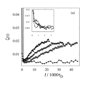
Finally, we explore the life time of a qSS of a self-gravitating system with a finite number of particles. To do this we define the crossover parameter
| (36) |
where is the number density of particles inside shells located between and at each time of simulation and where is the stationary distribution given by Eq. (19). The dynamical time scale is defined as . In Fig. 8a we plot the value of for systems with different number of particles. Fig. 8b shows that if we scale the time with , where , all the curves collapse onto one universal curve, showing the divergence of the crossover time in the thermodynamic limit. It is interesting to note that for a Hamiltonian Mean-Field (HMF) model, was found to diverge with the exponent Yama2004 , while for a virial 3d self-gravitating system the exponent was found to be . Unfortunately, at the moment there is no theory which allows us to predict this exponents a priory.
VIII Conclusions
We have studied the thermodynamics of 2d self-gravitating system in the microcanonical ensemble. It was shown that the gravitational clusters containing finite number of particles relax to the equilibrium state characterized by the MB distribution. Prior to achieving the thermodynamic equilibrium, however, these systems become trapped in a quasi-stationary state, where they stay for time , which diverges as for large . Thus, in the limit at fixed total mass , thermodynamic equilibrium can not be reached in a finite time. A new approach, based of the conservation properties of the Vlasov dynamics and on the theory of parametric resonances, is formulated and allows us to quantitatively predict the one particle distribution function in the non-equilibrium stationary state. Finally, it is curious to consider what will happen to a self-gravitating system in a contact with a thermal bath — the canonical ensemble. In Appendix B, it is shown that for a 2d self-gravitating system a stationary state is possible, if and only if, =1/2, i.e. when the kinetic temperature is . If such system is put into contact with a thermal bath which has there will be a constant heat flux from the reservoir into the system. This heat will be converted into the gravitational potential energy — since the kinetic energy is fixed by the virial condition — making the cluster expand without a limit. Conversely if the bath temperature is , the heat flux will be from the system into the bath. Again, since the system can only exist in a stationary state if , the energy for the heat flux can come only from the gravitational potential. In this case the gravitational cluster will contract without a limit, concentrating all of its mass at the origin. Thus, in the canonical ensemble no thermodynamic equilibrium is possible, unless the reservoir is at exactly . We hope that the present work will also help shed new light on the collisionless relaxation in 3d self-gravitating systems. Unfortunately the 3d problem is significantly more difficult, since besides the core-halo formation, one must also account for the particles evaporating to infinity.
This work was partially supported by the CNPq, INCT-FCx, and by the US-AFOSR under the grant FA9550-09-1-0283.
Appendix A The Total Energy
The gravitational potential energy of a system is
| (37) |
where the integration extends over all space. Unlike in 3d, the gravitational potential of a 2d system diverges at infinity. Therefore, some care must be taken with the limits. Performing the integration by parts we obtain
| (38) |
where is the radius of the bounding sphere. From Eq. (5), , and the total energy is given by
| (39) |
The divergence in the last term is common to all energy calculations in 2d. For example, if at the system is distributed with a water-bag distribution Eq. (8), its energy is
| (40) |
The gravitational self-energy in 2d is always divergent. However, since this divergence is always the same, it can be easily renormalized away. We simply add an infinite constant, , to all gravitational self-energies. The renormalized (finite) energy of a self-gravitating system is then
| (41) | |||
| . |
which for a water-bag distribution Eq. (8) becomes
| (42) |
Appendix B The Virial Theorem
The Hamiltonian of a general self-confined system is given by
where is the momentum of particle , and is the interaction potential. The virial function is defined as
Taking the time derivative, and using Hamilton’s equations we obtain
| (43) | |||||
where,
If is an homogeneous function of order
Euler’s theorem requires that
For a stationary state , and we obtain the usual result , where is the mean kinetic energy.
In two dimensions, is a sum of logarithms and Euler equation does not apply directly. However, we can still derive a 2d virial theorem by writing the inter-particle interaction potential as , which is a logarithm plus an infinite constant. This is a homogeneous function of order p=0, so we can use the Euler theorem to write
| (44) |
Note that since the right hand side of this equation only contains derivative of the potential, this expression is equally valid for and for the logarithmic potential. Substituting Eq. (44) into Eq. (43), we arrive at 2d virial theorem chav2006 .
| (45) |
In the thermodynamic limit, and after rescaling the velocity to put everything into adimensional form, we obtain the result , quoted in Section V.
Appendix C The Envelope Equation
We define the radius of the mass distribution as . Deriving twice with respect to time we obtain
| (46) |
This reduces to
| (47) |
where is the emittance which commonly appears in plasma physics Dav01 . The last term can be simplified using the Poisson equation (1) in its dimensionless form,
| (48) | |||||
which can be obtained directly using Eq. (5),
| (49) |
For a water bag initial distribution (8) we define the envelope radius as , so that for , and rewrites (47) as
| (50) |
This is the envelope equation. If initially, then and the envelope will not oscillate. This is precisely the virial condition.
Appendix D Potential for Core-Halo Distribution
Integrating the core-halo distribution function over velocity, the dimensionless Poisson equation (26) becomes
| (54) |
We define for , for , and for . Changing variables and , we can rewrite (54) as
| (55) |
The solution of the first two of these equations can be written in terms of the Bessel functions of first type and of order ,
| (56) | |||||
| (57) |
The last equation is solved by
| (58) |
where are the integration constants. The regularity of solution at the origin and Eq.(5) require that , and , respectively. The potential reduces to
| (59) | |||||
| (60) | |||||
| (61) |
where we have defined such that . The others requirements to continuity of the potential and its derivative are,
Solving these equations yields the integration constants as a function of and the parameters ,
| (63) | |||||
| (64) | |||||
| (65) |
The remaining equation of continuity of at and the conservation of energy will determine and , see Eq.(33).
References
References
- (1) J. W. Gibbs, Collected Works, Longmans, Green and Co., NY (1928).
- (2) J. Barré and D. Mukamel, and S. Ruffo, Phys. Rev. Lett. 87, 030601 (2001).
- (3) D. Lynden-Bell, Mon. Not. R. Astron. Soc. 136, 101 (1967).
- (4) W. Thirring, Zeitschrift für Physik, 235, Issue 4, pp.339-352 (1970).
- (5) D. Lynden-Bell and R. M. Lynden-Bell,, Mon. Not. R. Astron. Soc. 181, 405 (1977).
- (6) D. Mukamel, and S. Ruffo, and N. Schreiber, Phys. Rev. Lett. 95, 240604 (2005).
- (7) A. Ramírez-Hernández and H. Larralde and F. Leyvraz Phys. Rev. Lett. 100, 120601 (2008).
- (8) M.J. Klein, Phys. Rev. 97, 1446 (1955).
- (9) F. Bouchet and T. Dauxois Phys. Rev. E 72, 045103 (R) (2005).
- (10) Kavita Jain et al J. Stat. Mech. (2007) P11008
- (11) T. Padmanabhan, Physics Reports 188, 285 (1990); P.-H. Chavanis, Int. J. Mod. Phys. B 20, 22, 3113-3198 (2006).
- (12) Y. Levin, R. Pakter, and T. N. Teles, Phys. Rev. Lett. 100, 040604 (2008).
- (13) F. B. Rizzato, R. Pakter, and Y. Levin Phys. Rev. E 80, 021109 (2009).
- (14) P.-H. Chavanis, Physica D 200, 257 (2005).
- (15) J. Miller, Phys. Rev. Lett. 65, 2137â2140, (1990).
- (16) P. H. Chavanis and J. Sommeria, Journal of Fluid Mechanics, 314, pp 267-297.
- (17) A. Venaille and F. Bouchet, Phys. Rev. Lett. 102, 104501 (2009).
- (18) A. Campa, T. Dauxois, and S. Ruffo, Phys. Rep. 480, 57 (2009).
- (19) Y. Levin, R. Pakter, and F.B. Rizzato Phys. Rev. E. 78, 021130 (2008).
- (20) M. Joyce, B. Marcos, F. S. Labini, J. Stat. Mech. Theory and Experiment 2009, P04019 (2009).
- (21) Y. Levin, Rep. Prog. Phys. 65, 1577 (2002).
- (22) J. Ostriker, Astrophys. J. 140, 1056 (1964) ; J.J. Aly, Phys. Rev. E 49, 3771 (1994); J.J. Aly and J. Perez, Phys. Rev. E 60 5185 (1999)
- (23) W. Braun and K. Hepp, Comm. Math. Phys. 56, 101 (1977); A. Antoniazzi, F. Califano, D. Fanelli, and S. Ruffo, Phys. Rev. Lett. 98. 150602 (2007).
- (24) M. Antoni and S. Ruffo, Phys. Rev. E 52, 2361 (1995)
- (25) T. M. Rocha Filho, M. A. Amato, and A. Figueiredo J. Phys. A: Math. Theor. 42 165001 (2009).
- (26) T.N. Teles, R. Pakter, and Y. Levin, Applied Phys. Lett. 95, 173501 (2009).
- (27) R. L. Gluckstern, Phys. Rev. Lett. 73, 1247 (1994).
- (28) T. P. Wangler, K. R. Crandall, R. Ryne, and T. S. Wang, Phys. Rev. ST Accel. Beams 1, 084201 (1998).
- (29) M. Reiser, Theory and Design of Charged Particle Beams, (Wiley-Interscience, 1994); R.C. Davidson and H. Qin, Physics of Intense Charged Particle Beams in High Energy Accelerators (World Scientific, Singapore, 2001).
- (30) P.-H. Chavanis, Phys. Rev. E 73, 066103 (2006).
- (31) Y.Y. Yamaguchi, J.Barré, F.Bouchet, T.Dauxois, and S.Ruffo, Physica A (2004) 337, 36-66.