Realistic model atmosphere and revised abundances
of the coolest Ap star HD 101065

Abstract

Aims. Among the known Ap stars, HD 101065 is probably one of the most interesting objects, demonstrating very rich spectra of rare-earth elements (REE). Strongly peculiar photometric parameters of this star that can not be fully reproduced by any modern theoretical calculations, even those accounting for realistic chemistry of its atmosphere. In this study we investigate a role of missing REE line opacity and construct a self-consistent atmospheric model based on accurate abundance and chemical stratification analysis.

Methods. We employed the LLmodels stellar model atmosphere code together with DDAFit and Synthmag software packages to derive homogeneous and stratified abundances for 52 chemical elements and to construct a self-consistent model of HD 101065 atmosphere. The opacity in REE lines is accounted for in details, by using up-to-date extensive theoretical calculations.

Results. We show that REE elements play a key role in the radiative energy balance in the atmosphere of HD 101065, leading to the strong suppression of the Balmer jump and energy redistribution very different from that of normal stars. Introducing new line lists of REEs allowed us to reproduce, for the first time, spectral energy distribution of HD 101065 and achieve a better agreement between the unusually small observed Strömgren $c_{\rm 1}$ index and the model predictions. Using combined photometric and spectroscopic approaches and based on the iterative procedure of abundance and stratification analysis we find effective temperature of HD 101065 to be $T_{\rm eff}=6400$ K.

1 Introduction

Since its discovery by A. Przybylski in 1961 (Przybylski, 1961) and named later after him, the Przybylski’s star (HD 101065, hereafter PS) remains one of the most intriguing objects among Chemically Peculiar (CP) stars. These objects are usually characterized by abundance anomalies in their atmospheres and by non-uniform horizontal and vertical distributions of chemical elements and/or surface magnetic fields of different intensities.

From many observed characteristics PS is a typical representative of the coolest part of rapidly oscillating A-type (roAp) stars. It pulsates with the typical roAp period, $\approx$12 min (Kurtz & Wegner, 1979), and it was the first roAp star discovered. It possesses a $2.3$ kG surface magnetic field (Cowley et al., 2000) and its low Fe abundance (an order of magnitude below the solar value) follows the trend of Fe abundance versus effective temperature for Ap stars in 6300–14 000 K range (Kochukhov, 2003; Ryabchikova et al., 2004). A. Przybylski was the first to note a low Fe abundance and a strong overabundance of some rare-earth (REE) elements (Przybylski, 1966). These features were confirmed in many subsequent spectroscopic studies of this star (Wegner & Petford, 1974; Cowley et al., 1977; Cowley & Mathys, 1998; Cowley et al., 2000). For instance, in the latter study Cowley et al., (2000) reported an overabundance by up to $4$ dex (compared to the Sun) for elements heavier than Ni and enormously strong lines of the second ions of REEs compared to those of the first ions. This effect which is now commonly known as REE anomaly (Ryabchikova et al., 2001, 2004).

As new data for REE transitions becomes available via laboratory measurements, more lines of REEs are identified and measured in spectra of cool CP stars, thus improving abundance results. Later on it it was discovered that PS is not even a champion in REE overabundances. At least a couple of hotter Ap stars: HD 170973 – Kato, (2003); HD 144897 – Ryabchikova et al., (2006), with accurately derived REE abundances from numerous lines of the first and second ions have similar or even higher REE atmospheric overabundances. But a combination off a low temperature, low iron-peak abundances and large REE overabundances result in the extremely unusual observed spectrum of PS: weak lines of the iron-peak elements are lost in a forest of strong and numerous REE lines. For example, the typical density of only classified spectral features contributing to the theoretical spectra at $5375$ Å is 6–10 lines per Å, and still not enough for proper description of the PS spectrum since every second feature can not be accounted for in the modern spectrum synthesis.

Accurate spectroscopic analysis of PS requires dedicated model atmospheres. Indeed, abnormally strong REE absorption indicates that the atmospheric structure of the star may deviate significantly from that of normal, solar abundance stars. This is clearly seen, for instance, for the Strömgren $c_{\rm 1}$ photometric index that is close to zero, which is very different than for normal stars.

Previous attempt by Piskunov & Kupka, (2001) to account for peculiar absorption in the spectrum of PS and to fit color-indices based on the model atmosphere techniques faced a difficulty of the absence of complete line lists of REE and the impossibility to fit simultaneously photometric and spectroscopic features (like hydrogen lines) with the same model atmosphere. Piskunov & Kupka, (2001) used ATLAS9 (Kurucz, 1992, 1993) atmospheres with opacity distribution functions (ODF) recalculated for individual abundances and artificially enhanced line (but not continuum) opacity of iron to simulate the missing REE opacity. They finally adopted $T_{\rm eff}=6600$ K, $\log g=4.2$ model as a preferable choice for spectroscopic analysis. However, this model failed to explain peculiar photometric parameters of the star. Enhanced metallicity model by Piskunov & Kupka, (2001) lead to the decrease of $c_{\rm 1}$ index but its theoretical magnitude is still too high compared with the observed value. This model was used in extensive abundance study of PS by Cowley et al., (2000).

Another striking evidence of the abnormality of the atmospheric structure of PS is the presence of the so-called core-wing anomaly in the hydrogen Balmer lines (Cowley et al., 2001). This abrupt transition between the Doppler core of the hydrogen lines and their Stark wings has been modeled empirically by Kochukhov et al., (2002) in terms of a temperature increase by 500–1000 K at intermediate atmospheric heights but so far has not been explained theoretically.

Thus, HD 101065 remains an extremely challenging and very intriguing target for the application of advanced model atmosphere analysis and high-resolution spectroscopy. In this paper we present a new attempt to combine both of these approaches and to construct a self-consistent model atmosphere of PS taking into account realistic chemistry of its atmosphere and employing up-to-date theoretical calculations of the spectra of selected REEs.

Starting with a brief description of observations in Sect. 2, we then present methods of analysis in Sect. 3 and describe the new lists of REE lines employed in the model atmosphere calculations. Results of our analysis are presented in Sect. 4 and are followed by general conclusions in Sect. 5. Our paper concludes with a brief discussion in Sect. 6.

2 Observations

In our study we employed several existing spectra of PS: NTT spectrum with the resolving power $R\approx 80\,000$ in the $3950-6630$ Å wavelength region, (Cowley et al., 2000), UVES spectrum in the $3100$–$10\,000$ Å region with the resolving power $R\approx 80\,000$ (Kochukhov et al., 2002; Ryabchikova et al., 2008), and an averaged UVES spectrum from the time-series observations obtained in the 4960–6990 Å spectral region with the resolving power $R\approx 115\,000$ (Kochukhov et al., 2007; Ryabchikova et al., 2007).

Details of the spectroscopic observations and full description of the data reduction are given in the corresponding papers. Direct comparison of the normalized spectra reveals a remarkable agreement between all observations. This allows us to use the equivalent width measurements from Cowley et al., (2000), supplementing them with the measurements in the spectral region $\lambda>6600$ Å using the other two spectra.

3 Methods

3.1 Abundance analysis

The main goal of the present paper is to calculate a model atmosphere of PS accounting for its anomalous chemical composition. In magnetic chemically peculiar star an accurate abundance analysis may be carried out by fitting the magnetic synthetic spectrum to the observed line profiles. This procedure is very time consuming. Therefore, to simplify calculations, we analysed the equivalent widths replacing magnetic effects by a pseudo-microturbulence. It is sufficient for line opacity calculations, although the abundances derived using the common value of microturbulent velocity may be slightly inaccurate (see discussion in Cowley et al., 2000). In present analysis we used the Kurucz, (1993) WIDTH9  code modified by V. Tsymbal (see Ryabchikova et al., 1997).

The VALD database (Piskunov et al., 1995; Kupka et al., 1999) and the DREAM REE line database (Biémont et al., 1999, and references therein), which is made accessible via the VALD extraction procedures, are our main sources for atomic parameters. For the REE, which provide the majority of lines in the PS spectrum, accurate laboratory transition probabilities measured by Wisconsin group are used: Lawler et al., 2001a – La ii; Lawler et al., 2001a – La ii; Lawler et al., (2009) – Ce ii; Den Hartog et al., (2003) – Nd ii; Lawler et al., (2006) – Sm ii; Lawler et al., 2001b – Eu ii; Den Hartog et al., (2006) – Gd ii; Lawler et al., 2001c – Tb ii; Wickliffe et al., (2000) – Dy i/Dy ii; Lawler et al., (2008) – Er ii; Wickliffe & Lawler, (1997) – Tm ii; Lawler et al., (2007) – Hf ii. Among heavier elements Th and U are particularly interesting. For these species we used laboratory and calculated transition probabilities from the following papers: Nilsson et al., 2002a – Th ii; Biémont et al., (2002) – Th iii; Nilsson et al., 2002b – U ii. Transition probabilities for REEs in the second ionization stage were taken from the DREAM database except Pr iii Mashonkina et al., (2009), Nd iii Ryabchikova et al., (2006), Eu iii Wyart et al., (2008), Tb iii and Dy iii (Ryabtsev, private communication).

Extended measurements and theoretical calculations for the REEs, Th and U justify revision of some of the partition functions (PF), which until now mainly came from Kurucz, (1993) ATLAS9 code. Our recalculated PFs are made available online.

We did not take into account the hyperfine structure (hfs) in our abundance analysis because the hfs constants are available only for a small subset of spectral lines.

3.2 Stratification analysis

In the majority of cool Ap stars the atmospheres are not chemically homogeneous. Element stratification built up by atomic diffusion influences the atmospheric structure (Shulyak et al., 2009; Kochukhov et al., 2009; Leblanc et al., 2009). As it follows from Khan & Shulyak, (2007), Fe, Si, and Cr are the elements that have the major effect on the atmospheric $T-P$ structure in the case of homogenous abundances. The cumulative effect of element stratification on the model structure was demostrated by Wade et al., (2003) and later by Monin & LeBlanc, (2007) who used diffusion calculations for $39$ chemical elements simultaneously. Thus, the stratification analysis of PS was performed for four elements: Fe, Ba, Ca, and Si. It was not possible to carry out stratification analysis for Cr and other iron-peak elements due to weakness of their absorption features and heavy blending by REE lines. The lower energy levels of practically all Cr lines used in the abundance determination belong to a narrow energy range, which makes the Cr lines insensitive to abundance gradients. Hence, we restricted stratification analysis to the four elements since they are represented in HD 101065 by a sufficient number of atomic lines, probing different atmospheric layers and enabling line profile fitting.

We applied a step-function approximation of chemical stratification as implemented in DDAFit – an automatic procedure for determination of vertical abundance gradients (Kochukhov, 2007). In this routine, the vertical abundance distribution of an element is described by four parameters: chemical abundance in the upper atmosphere, abundance in deep layers, the position of the abundance jump and its width. All four parameters can be optimized simultaneously with the least-squares fitting procedure.

Most unblended lines in the PS spectrum are located in the red spectral region, where line profiles are also substantially distorted by the Zeeman splitting due to wavelength dependence of the Zeeman effect. DDAFit enables an accurate stratification analysis of such magnetically-splitted lines. In the search for optimal vertical distribution of chemical elements we use magnetic spectrum synthesis with the Synthmag code (Kochukhov, 2007). This software represents an improved version of the program developed by Piskunov, (1999).

A list of the lines used in stratification analysis is given in Table 3 (Online material). To get a better sensitivity of the fitted Ca distribution to the upper atmospheric layers, we used the IR-triplet Ca ii line at $\lambda$ 8498 Å. As shown by Ryabchikova et al., (2008) and Cowley et al., (2009), its core is represented entirely by the absorption of the heavy isotope ⁴⁸Ca. Therefore wavelength of the line of this isotope is given in Table 3.

3.3 Calculation of model atmospheres

To perform the model atmosphere calculations we used the recent version of the LLmodels  (Shulyak et al., 2004) stellar model atmosphere code. The code accounts for the effects of individual and stratified abundances. The stratification of chemical elements is an input parameter and thus does not change during the model atmosphere calculation process. This allows us to explore the changes in the model structure due to stratification that was inferred directly from observations, without modeling poorly understood processes that could be responsible for the observed inhomogeneities.

Note that such an empirical analysis of chemical element stratification is based on the model atmosphere technique and thus the temperature-pressure structure of the model atmosphere itself depends upon the stratification which we want to determine. Therefore, the calculation of the model atmosphere and the stratification (abundances) analysis are linked together and an iterative procedure should be used in this case. It consists of repeated steps of stratification and abundance analysis that provide an input for the calculations of model atmosphere until atmospheric parameters ($T_{\rm eff}$, $\log g$, etc.) converge and theoretical observables (photometric colors, profiles of hydrogen lines, etc.) fit observations. We refer the reader to the recent papers (Shulyak et al., 2009; Kochukhov et al., 2009) for a more detailed description of this technique.

The VALD database (Piskunov et al., 1995; Kupka et al., 1999) was used as a main source of the atomic line data for computation of the line absorption coefficient. The recent VALD compilation contains information on about $66\times 10^{6}$ atomic transitions. Most of them come from the latest theoretical calculations performed by R. Kurucz.

Since a $2.3$ kG surface magnetic field of PS is too weak to affect noticeably the atmospheric structure and energy distribution (see Kochukhov et al., 2005; Khan & Shulyak, 2006, for more details) we adopted a $1$ km s^-1microturbulent velocity to roughly account for the magnetic broadening and to avoid time-consuming model calculations with detailed polarized radiative transfer.

3.4 REE line lists for model atmosphere calculation

The main sources for the REEs transition probabilities data between experimentally known energy levels are VALD  and DREAM  databases, hereafter referred to “VALD data”. These data were supplemented by the transition probabilities for the observed and predicted lines of Pr ii-Pr iii (Mashonkina et al., 2009), Nd ii-Nd iii (Mashonkina et al., 2005; Ryabchikova et al., 2006), Eu iii (Wyart et al., 2008), Tb iii and Dy iii (Ryabtsev, private communication), hereafter referred to as “ISAN data”. For the latter two ions transition probability calculations were based on the extended term analysis.

Table 2 demonstrates a dramatic difference between the number of observed (VALD) and predicted (ISAN) transitions for Pr and Nd, in particular for the lines of the first ions. We are missing more than 90%  of the potential line absorbers. The same situation is expected for lines of the other REEs. Taking this situation into account, we performed calculations for Sm ii – the second-abundant element after Nd in PS. The energy levels of Sm ii were calculated by the Hartree-Fock method implemented in the Cowan, (1981) code. The ground state of Sm ii is the 4f⁶6s configuration. In addition, our calculations include even configurations 4f⁶nd (n=5,6), 4f⁶7s, 4f⁵5d6p, 4f⁵6s6p, and odd configurations 4f⁶np (n=6-8), 4f⁴5d²6p, 4f⁴6s²6p, 4f⁵5d², 4f⁵5d6s. Calculations are based on the wave functions obtained by the fittings the energy levels. As in the case of Pr ii and Nd ii, all Hartree-Fock transition integrals are scaled by a factor 0.85. In total, transition probabilities for more than one million lines were calculated and added to the ISAN list of the REE lines.

The recent studies by Mashonkina et al., (2005, 2009) demonstrated that the line formation of Pr and Nd can strongly deviate from the local thermodynamic equilibrium. For instance, the doubly ionized lines of these elements are unusually strong due to combined effects of stratification of these elements and departures from LTE. However, a precise NLTE analysis is beyond the scope of this paper and currently could not be coupled to a model calculation. Therefore, we followed the approach outlined in Shulyak et al., (2009) where authors used a simplified treatment of the REE NLTE opacity.

Taking into account a systematic difference in abundances derived for the first and second REE ions, it is essential to reduce the oscillator strengths for the singly ionized REE lines by this difference in the model line list while using the abundances derived from second ions as an input for model atmosphere calculations (or vice versa). Obviously, the adopted reduction factors depend upon the assumed abundances of the first and second ions and thus change slightly if the model parameters ($T_{\rm eff}$, $\log g$, etc.) are modified in the course of the iterative procedure of abundance analysis. The logarithmic scaling factors, $\log(N_{\rm II}/N_{\rm III})$, adopted for our final model are (in dex): $-1.6$ (Ce), $-2.4$ (Pr), $-1$ (Nd), $-2.66$ (Tb), $-2.5$ (Dy), and $-1.64$ (Eu). These factors were applied to all lines of the respective ions in the master line list. Then this line list was processed by the line pre-selection procedure in the LLmodels code to select only those lines that contribute non-negligibly to the total line opacity coefficient for a given temperature-pressure distribution. Applying this line scaling procedure allowed us to mimic the line strengths correspond to the NLTE ionization equilibrium abundance for each REE (see Shulyak et al., 2009, for more details).

4 Results

4.1 Adopted atmospheric parameters

We started analysis with a homogeneous abundance model calculated with $T_{\rm eff}=6600$ K, $\log g=4.2$, and individual abundances taken from Cowley et al., (2000). Once the stratification was introduced in the model atmosphere, the fit to the hydrogen H$\alpha$ line and the observed photometric parameters required decreasing of $T_{\rm eff}$ of the star down to approximately $6400$ K. In total, four iterations of the abundance analysis and the model atmosphere calculation were performed to achieve a converged solution. The abundances from the third iteration did not introduce noticeable changes in the atmospheric structure.

The effective temperature obtained in our study is identical to the $T_{\rm eff}$ obtained by Kochukhov et al., (2002), who fitted the H$\alpha$ and H$\beta$ lines using the same UVES spectra. However, Kochukhov et al. relied on less advanced ATLAS9 model atmospheres calculated using ODFs with artificially increased Fe line absorption (Piskunov & Kupka, 2001) and also attempted to empirically adjust the $T$-$\tau$ structure of their model.

Figure 1 illustrates the observed and predicted H$\alpha$ line profiles calculated with different atmospheric models. Unfortunately, it is impossible to infer an accurate value of $\log g$ from the H$\alpha$ profile due to low temperature of the star and resulting poor sensitivity of the hydrogen lines to the pressure stratification. For this reason we kept this parameter fixed during the iterative procedure of abundance analysis (however, see Discussion).

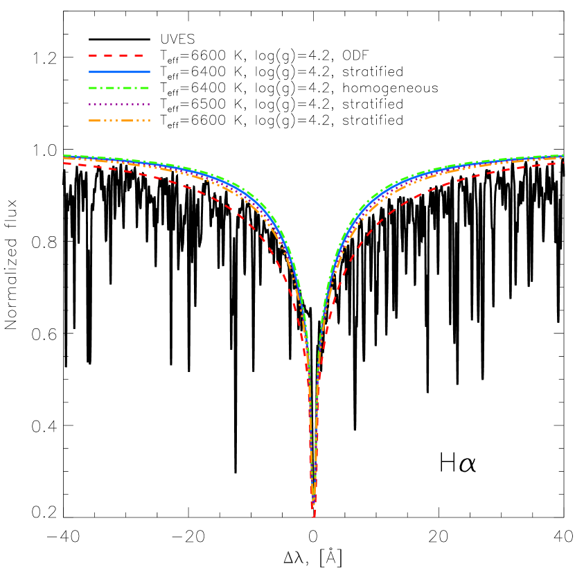
Figure 1: Comparison between the observed and predicted H$\alpha$ line profiles.

4.2 Abundance pattern

Table 4 (Online material) summarizes individual abundances of chemical elements in the atmosphere of PS derived with the final model atmosphere. Note the strong enrichment of REE elements compared to the solar composition. These elements dominate the spectrum of PS, playing a key role in the radiative energy balance (see below).

In Fig. 2 we illustrate abundance pattern of PS relative to the recent compilation of the solar abundances (Grevesse et al., 2007). The elements heavier than Ba exhibit an overabundance by 3 dex and larger. Several REEs show clear ionization anomaly related to stratification of these elements and departures from LTE.

Vertical distribution of Si, Fe, Ba, and Ca is presented in Fig. 3. This figure illustrates the difference between the initial and final stratification as derived at the first and the last iterations respectively. Ba seems to be the only element whose stratification did not change appreciably during iterations. Only the position of the abundance jump changed slightly. Fe shows a change in the abundance in the upper atmosphere by about $\sim$ 1 dex. The position of the abundance jump for Si changed significantly. In contrast, the Ca abundance in the upper atmosphere changes dramatically. These results illustrate the importance of taking into account a feedback of stratification on the model structure.

The effect of introducing stratification on the fit to H$\alpha$ line appears to be not very strong. The maximum difference between the stratified and non-stratified model predictions is at the level of $1$% as seen from Fig. 1. However, the two profiles are still clearly distinguishable. Thus, chemical stratification should be taken into account in accurate modeling of the hydrogen line formation.

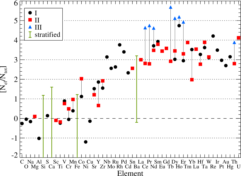
Figure 2: Chemical composition of the atmosphere of HD 101065. Different symbols correspond to ions from I to III. Bars show abundance ranges for stratified elements.

The Fe and Ba abundance distributions agree with those derived previously by either trial-and-error method (Ryabchikova, 2003) or based on the equivalent widths (Yushchenko et al., 2007). Figures 4-7 (Online material) illustrate the resulting fit to line profiles.

Figure 3: Stratification of four elements in the atmosphere of HD 101065 derived at the first and last iteration of the abundance analysis.

3

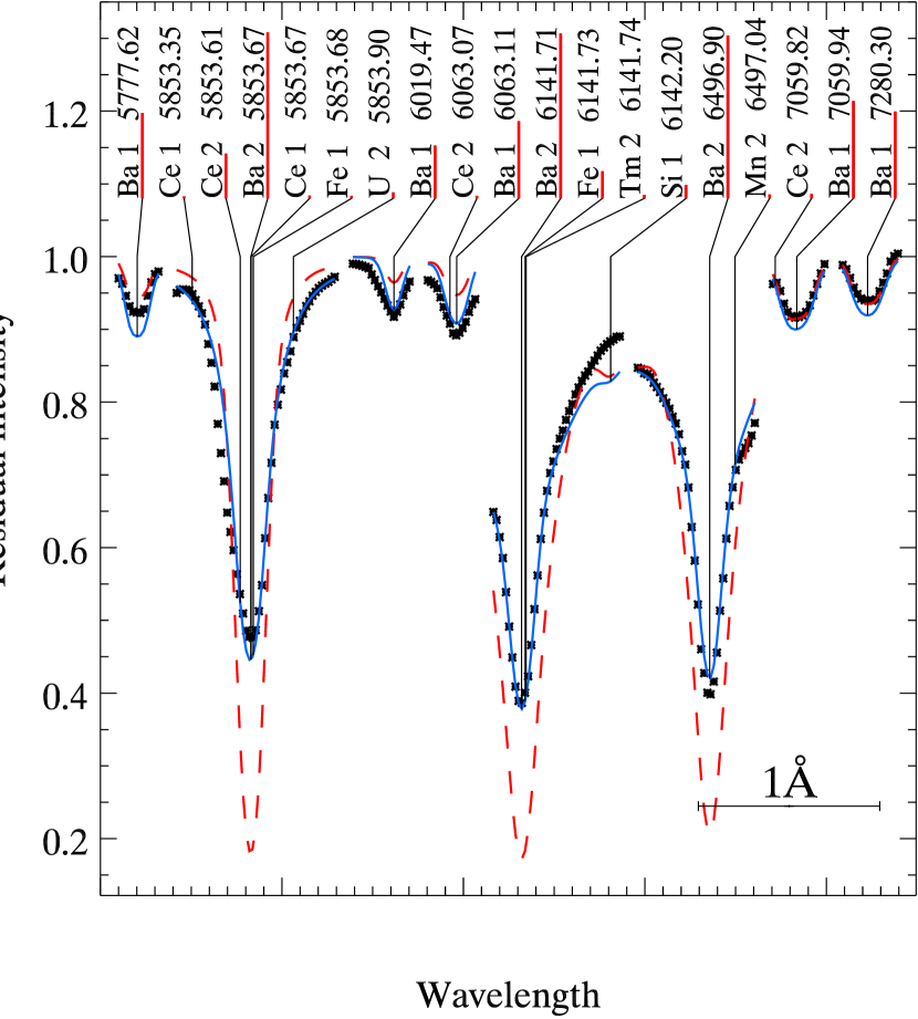
Figure 4: Comparison between the observed and theoretical profiles for the Ba lines. Observations are shown with symbols, thick full line corresponds to the synthetic spectrum calculated with the best-fitting stratified abundance distribution and dashed line shows prediction of the spectrum synthesis with a homogeneous abundance.

4

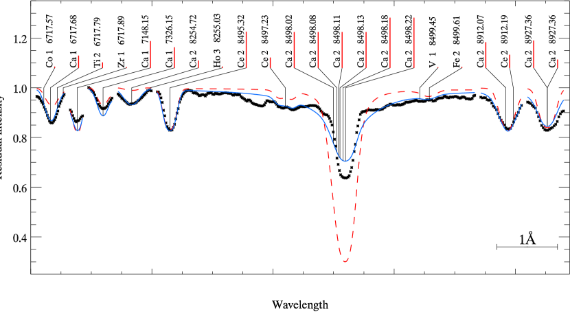
Figure 5: Same as in Fig 4 but for Ca.

5

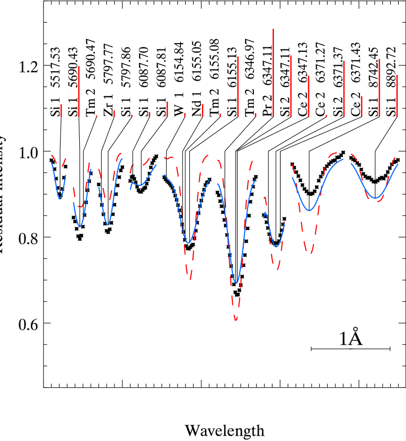
Figure 6: Same as in Fig 4 but for Si.

6

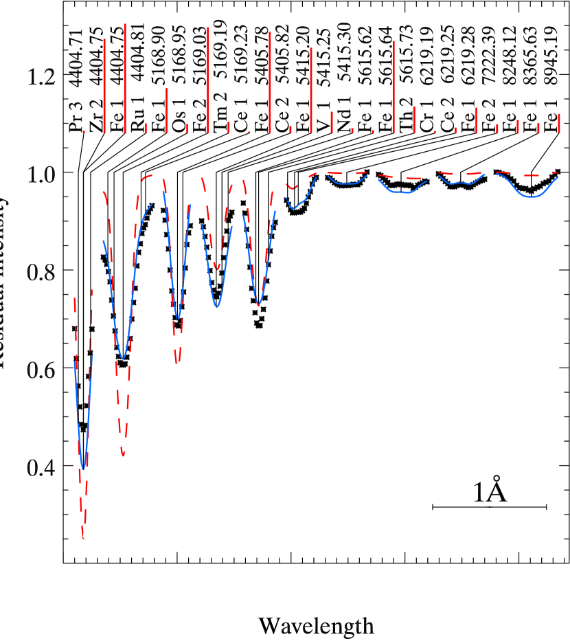
Figure 7: Same as in Fig 4 but for Fe.

4.3 Energy distribution and photometric colors

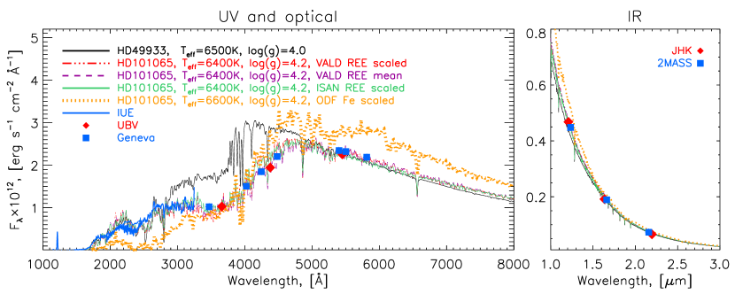
Figure 8: Observed and theoretical energy distribution of HD 101065 calculated using line lists from two datasets: VALD and ISAN. For comparison purpose the theoretical energy distribution of a normal F-type star HD 49933 is also shown. All theoretical calculations are smoothed with $20$Å Gaussian.

Unusual photometric parameters of PS clearly indicate that its energy distribution should differ much from that of normal stars with similar $T_{\rm eff}$. Indeed, a dense forest of REE lines obtained from theoretical computations should have a strong impact on the atmospheric energy balance.

Figure 8 illustrates theoretical energy distributions of HD 101065 and a normal F-type star HD 49933. Both stars have close effective temperatures but very different atmospheric chemistry: HD 49933 has a slight underabundance of iron-peak elements and a nearly solar abundance of REEs as derived by Ryabchikova et al., (2009). Model fluxes were computed with the stratified distribution of Si, Ca, Fe, and Ba as well as with the scaled REE abundances as described above. In addition, ATLAS9 ODF model from Piskunov & Kupka, (2001) calculated with $T_{\rm eff}=6600$ K, $\log g=4.2$ and Fe opacity scaled to simulate an enhanced REE absorption is shown for comparison purpose. To keep the figure representative, here we show only models with final $T_{\rm eff}=6400$ K, $\log g=4.2$ and different assumptions about REE opacity. Energy distributions of models with $T_{\rm eff}=6500$ K and $T_{\rm eff}=6600$ K are displayed in Fig. 9 (Online Material).

8

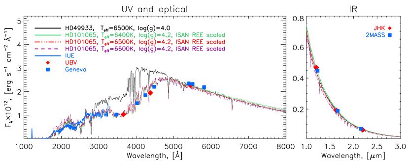
Figure 9: Observed and theoretical energy distribution of HD 101065 calculated with scaled REE opacity from ISAN line list (see text). For comparison purpose the theoretical energy distribution of a normal F-type star HD 49933 is also shown. All theoretical calculations are smoothed with $20$Å Gaussian. Theoretical fluxes were scaled assuming radiuses: $R=1.98R_{\odot}$ for HD 49933 and $T_{\rm eff}=6400$ K models; $R=1.90R_{\odot}$ for $T_{\rm eff}=6500$ K; $R=1.82R_{\odot}$ for $T_{\rm eff}=6600$ K.

The observed energy distribution of PS is constructed combining the large-aperture IUE observations extracted from the INES database and photometric data in the $UBV$ (Wegner, 1976), Geneva, $JHK$ (Catalano et al., 1998) and $2MASS$ (Skrutskie et al., 2006) systems converted to absolute fluxes. The model fluxes are scaled to account for the distance to PS, which is $112\pm 11$ pc according to the revised Hipparcos parallax of $\pi=8.93\pm 0.87$ mas (van Leeuwen, 2007). Theoretical fluxes are further scaled to match the observed Paschen continuum defined by the $UBV$ and Geneva photometry. This scaling factor corresponds to the radius of the star, for which we found $R=1.98\pm 0.03R_{\odot}$. The same scaling is applied to all theoretical fluxes presented in Fig. 8. For models with $T_{\rm eff}=6500$ K and $T_{\rm eff}=6600$ K we find $R=1.90R_{\odot}$ and $R=1.82R_{\odot}$ respectively (see Fig. 9, Online Material).

It is evident that the enormous REE absorption leads to smoothing of the Balmer jump. This is clearly visible for both models computed with the new ISAN REE line list and with the original VALD REE line list. The only difference is that the former one predicts less flux redward of $4100$Å and more flux in the region $3000$Å and $3800$Å (note that the model computed with mean REE abundances should be used with big caution due to ignoring REE anomaly, and we present it in Fig. 8 for illustrative purpose only). Taking into account difficulties in predicting accurately the spectra of REEs, one can conclude that our models computed with the recent improvements of the line REE opacity provide a reasonably good fit to the observed fluxes. They are able to reproduce not only the shape of the observed energy distribution but also the amplitude of the Balmer jump reasonably well, much better than in the previous attempt by ODF-based modeling (Piskunov & Kupka, 2001). However, there are still some discrepancies with observations, i.e. too high fluxes in the 2000–2500 Å region and around 4500 Å. The description of the energy distribution of PS can be probably improved in the future once more complete line lists of REEs will become available. A new well-calibrated observed spectrophotometry in the 3300–10 000 Å region would also be extremely useful for further modeling.

The impact of the peculiar energy distribution on the photometric parameters of HD 101065 is illustrated in Table 1. Observations in the Strömgren system were taken from Hauck & Mermilliod, (1998). Predictions of Piskunov & Kupka, (2001) model calculated with the ODF line opacity representation using abundances from (Cowley et al., 2000) are also given for comparison. We also show theoretical photometric parameters for the models calculated with the mean REE abundances corresponding to the first and second ions, as well as for the models with the scaled REE opacity, and for different $T_{\rm eff}$. All models except the ODF-based one were computed with the chemical stratification illustrated in Fig. 3.

There are few things to note from Table 1. First of all, a strong impact of the REE opacity is clearly seen for the $c_{\rm 1}$ photometric index which reaches an even more negative value than the observed one for the models with the ISAN data and the mean REE abundances. Similarly, the recent version of VALD already provides REE opacity that is enough to bring down $c_{\rm 1}$ index significantly compared to previous calculations and provides a result very close to the observed one. However, mean abundances can not be used for accurate modeling due to significant REE ionization anomaly. Accounting for this via the scaling of REE line opacity decreases the flux redistribution effect and thus the impact on the $c_{\rm 1}$ index. The implementation of the new ISAN data gives a much better fit to observations than using the data from VALD alone, yet this fit is far from being fully satisfactory.

Second, it remains difficult to obtain a good fit simultaneously for all photometric indices. For instance, all models fail to reproduce the $U-B$ value, while $b-y$ is not reproduced by models with the scaled REE opacity unless one decreases $T_{\rm eff}$ to $\approx$ 6200 K. However, lowering $T_{\rm eff}$ is not consistent with the observed H$\alpha$ line. Similar, worse fit is obtained for models with $T_{\rm eff}>6400$ K, which show reduced $b-y$ and increased $c_{\rm 1}$ indicies.

Third, stratification of Fe, Si, Ca, and Ba considered in our study does not play a significant role for the overall energy redistribution and thus photometric colors as seen from the sixth raw of Table 1. Most of the photometric indicators are negligibly affected by the presence of stratification. The $c_{\rm 1}$ index is again an exception since it decreases by $\approx$ 0.03 mag if stratification is introduced. However, this change is still fairly small compared to typical precision of the observed Strömgren photometry.

Finally, a high sensitivity of the photometric parameters to the new ISAN calculations indicates that the general disagreement between models and observations is the subject of future more precise and complete calculations of REE spectra. Using the data for more REE elements than those presented in this investigation can potentially improve the fit to the highly peculiar observed photometric properties of PS. Implementation of the ISAN line lists for only a few REE ions already allowed us to achieve significantly better results compared to previous modeling attempts and clearly showed that the “enigmatic” characteristics of PS likely result from the REE line opacity which was ignored in previous calculations. We can thus suggest that further step in the modeling of the observed properties of PS should be made in the direction of improved theoretical calculations of REE transitions.

Table 1: Observed and predicted colors of HD 101065.

	$b-y$	$m_{\rm 1}$	$c_{\rm 1}$	$B-V$	$U-B$
Observations	$\mathbf{0.442}$	$\mathbf{0.427}$	$\mathbf{-0.013}$	$\mathbf{0.760}$	$\mathbf{0.200}$
t6600g4.2, ODF	$0.387$	$0.582$	$0.298$	$0.767$	$0.571$
t6400g4.2
VALD	$0.440$	$0.439$	$0.029$	$0.745$	$0.268$
REE mean abun.
t6400g4.2
ISAN	$0.456$	$0.587$	$-0.202$	$0.829$	$0.379$
REE mean abun.
t6400g4.2
VALD	$0.394$	$0.420$	$0.312$	$0.681$	$0.368$
REE scaled abun.
t6400g4.2
ISAN	$0.384$	$0.413$	$0.158$	$0.663$	$0.274$
REE scaled abun.
t6500g4.2
ISAN	$0.367$	$0.397$	$0.200$	$0.634$	$0.255$
REE scaled abun.
t6600g4.2
ISAN	$0.350$	$0.391$	$0.229$	$0.607$	$0.240$
REE scaled abun.
t6400g4.2
ISAN, hom.	$0.383$	$0.396$	$0.188$	$0.656$	$0.271$
REE scaled abun.
t6200g4.5
ISAN	$0.417$	$0.444$	$0.024$	$0.719$	$0.261$
REE scaled abun.

All models were computed with stratification of Fe, Si, Ca, and Ba, except those marked as “ODF” and “hom.”

The strong suppression of the Balmer jump and energy redistribution to the infrared is a direct result of the unusually high REE abundances in the stellar atmosphere. Table 2 summarizes some statistics illustrating importance of the REE opacity in the atmosphere of PS. It shows the number of lines of a given ion before and after line preselection procedure performed by the LLmodels code. This procedure selects from the master line list only those lines that noticeably contribute to the line opacity for a given $T$-$P$ structure. Usually the preselection criterion is $\kappa_{\rm line}/\kappa_{\rm cont}>1\%$, where $\kappa_{\rm line}$ and $\kappa_{\rm cont}$ are the line center and continuum opacity coefficients, respectively. It is seen that, for instance, all lines of Pr ii and Nd ii present in the current version of VALD contribute to the opacity in the atmosphere of PS. A larger number of lines is selected from the more complete ISAN line lists.

Table 2: Summary of REE lines in VALD and combined ISAN line lists before and after line preselection procedure.

	Pr ii	Pr iii	Nd ii	Nd iii	Sm ii	Eu iii	Dy iii	Ce ii	Ce iii
Original
VALD	$510$	$19104$	$1285$	$71$	$1346$	$893$	$1313$	$16046$	$2966$
ISAN	$103428$	$---$	$1172579$	$6858$	$1047088$	$23827$	$31121$	$---$	$---$
After preselection with $1$% limit for $T_{\rm eff}=6400$ K, $\log g=4.2$ model, REE scaled abundances
VALD	$510$	$6539$	$1285$	$71$	$1121$	$58$	$1134$	$15908$	$1270$
ISAN	$83167$	$---$	$74413$	$3810$	$58637$	$74$	$21715$	$---$	$---$

As expected from the low magnitude of the $c_{\rm 1}$ index and the energy distribution shown in Fig. 8, a great majority of strong REE lines are concentrated around the Balmer jump. Figure 10 illustrates the line distribution for selected REE ions depending upon their wavelength position and central intensity. We show the number of lines per 50 Å wavelength bin for which the central intensities are greater or equal to a given normalized intensity. The latter ranges from $0$ (fully saturated strong line) to $1$ (continuum level, weak line). One can seen that ions like Ce ii, Pr ii, Nd ii/iii, Sm ii have a large number of strong lines located exactly in the region of Balmer jump and blueward, dramatically contributing to the opacity and radiation field.

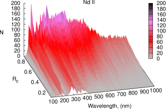
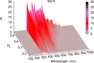
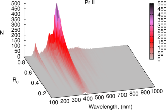
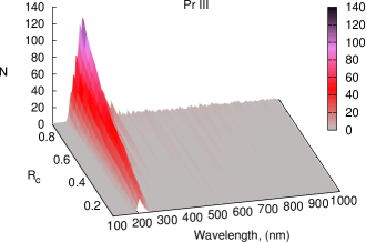
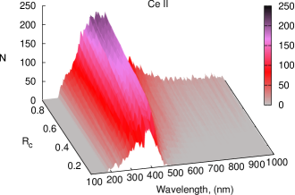
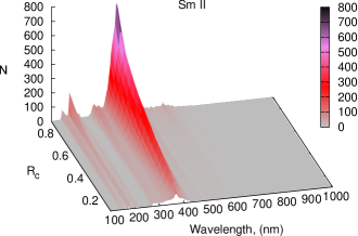
Figure 10: Distribution of lines for several REE ions depending on their position and central depth in the ISAN line lists for the model atmosphere with $T_{\rm eff}=6400$ K, $\log g=4.2$.

5 Conclusions

HD 101065 is known to be one of the most peculiar stars ever found. Its unusual photometric colors and extremely rich spectra of REE elements represent a major challenge for modern stellar atmosphere theory. With the increasing number of the accurately measured and calculated REE transitions and the progress in the model atmosphere techniques it became possible to carry out this quantitatively new analysis of the spectrum of HD 101065 and to re-determine atmospheric parameters of this star.

In this study we investigated the impact of the new theoretically computed spectra of some REE elements on the atmospheric properties of HD 101065 and carried out a detailed spectroscopic analysis of the stratification of Si, Fe, Ba, and Ca in the stellar atmosphere. Theoretical computations of REE transitions have extended already existing line lists of REE lines by a factor of one thousand. Implementing an iterative procedure of the abundance analysis, we re-derived atmospheric parameters of the star in a self-consistent way, accounting for the ionization disequilibrium between the first and second ions of the REEs caused by significant NLTE effects.

The main results of our investigation can be summarized in the following:

• REEs appear to play a key role in the radiative energy balance in the atmosphere of HD 101065, leading to the strong suppression of the Balmer jump and energy redistribution from UV and visual to IR.

• The abnormal photometric color-indices of HD 101065 arise due to a strong absorption in REE lines. We showed that the introduction of the new extensive line lists of REEs allow one to achieve a better agreement between the unusually low magnitude of the Strömgren $c_{\rm 1}$ index observed for this star and the model predictions. We also demonstrated, for the first time, a satisfactory agreement between the observed and computed spectral energy distribution of HD 101065.

• The remaining discrepancy between the observed and calculated photometric parameters indicates that some important opacity sources are still missing in the modeling process. For this reason the future extension of the REE line lists is needed for complete understanding of the observed properties of HD 101065.

• Using theoretical spectrum synthesis we derived stratification profiles for Si, Ca, Fe, and Ba. We found a strong depletion of all these elements in the upper atmosphere of HD 101065. The effect of stratification on the H$\alpha$ line profile appears to be at the level of $1$%, which is however important for accurate calculation of the hydrogen line profiles.

• There is not much influence of the stratification on the considered photometric parameters of HD 101065, except for the Strömregn $c_{\rm 1}$ index, which is modified by stratification by $0.03$ mag.

• Using combined photometric and spectroscopic analysis and based on our novel iterative procedure of the abundance and stratification analysis we find effective temperature of the HD 101065 to be $T_{\rm eff}=6400$ K.

Taking into account the current progress in the atmospheric modeling, understanding of the REE opacity, and detailed spectroscopic analysis we conclude that there is nothing special in HD 101065 compared to other known cool Ap and roAp stars except its relatively low $T_{\rm eff}$ and a high abundance of REEs. Consequently, for this moment HD 101065 appears to be the coolest Ap and roAp star known but otherwise is a typical member of these groups.

6 Discussion

We can compare the global parameters of HD 101065  derived in the present study with the values obtained by an independent pulsation modeling (Mkrtichian et al., 2008). The best model explaining the observed frequency pattern of HD 101065  is characterized by $T_{\rm eff}$ = 6622$\pm$100 K, $\log g$ = 4.06$\pm$0.04, R = $1.90\pm 0.08$ $R_{\odot}$. These parameters agree with ours within $2\sigma$. However, to fit the observed frequencies in the framework of current asterosismic models one needs dipolar magnetic field strength $B_{\rm p}$ = 8.7 kG, which is incompatible with the observed field modulus of $\langle B\rangle$ = 2.3 kG. One of the reasons for this significant discrepancy between the observed and inferred magnetic field is the use of normal $T$-$\tau$ relation in the pulsation modeling. This relation differs significantly from a more realistic one derived in the present paper, as illustrated in Fig. 11 (Note that computing model with solar abundances we did not apply scaling of the REE opacity due to the low abundance of REE elements in solar atmosphere and thus its negligible impact on model structure). As expected from the fit to H$\alpha$ line and photometric parameters presented above, the effect of stratification on model $T-P$ structure is negligible and hardly distinguishable from the homogeneous abundance model (dash-dotted line in Fig. 11). Note that it is still considereably different from the solar abundance model, and is in good agreement with the result of Monin & LeBlanc, (2007).

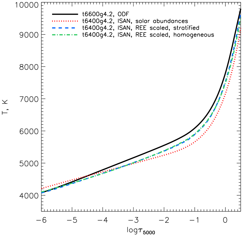
Figure 11: Comparison in atmospheric temperature structure of theoretical models. Thick line –  ODF model from Piskunov & Kupka, (2001), dotted line – homogeneos solar abundances model, dashed line – stratified abundances final model adopted in the present study, dash-dotted line – same as before but assuming homogeneos abundances.

In spite of our new results, illustrating an improved understanding of the physics of the atmosphere of HD 101065, it is still impossible to describe all observed properties of this star with the current state-of-the-art modeling. In this section we would like to discuss physical effects that we ignored in our analysis.

Taking into account a jungle of the REE lines seen in the spectrum of HD 101065 and their importance as an opacity source for the model atmosphere calculation it would be reasonable to search for the possible stratification of rare-earth elements. Considering the case of a hotter roAp star HD 24712, for which the accumulation of REEs in the upper atmosphere plays a critical role, producing a characteristic inverse temperature gradient (see Shulyak et al., 2009, for more details), one would expect the same mechanism to operate in the atmosphere of HD 101065 as well. However, the stratification analysis of REEs is highly complicated due to blending of REE lines with accurately known atomic parameters (that ideally should be used for such an analysis) by other REE lines for that no laboratory measurements exist and thus can not be included in the spectrum synthesis. At the same time, assuming that REEs are distributed similarly in both stars, we do not expect a strong impact of the REE stratification on the energy distribution of HD 101065 simply because it would affect only the optically thin atmospheric layers.

As mentioned above, due to the low $T_{\rm eff}$ of PS, it is impossible to infer the $\log g$ value from the hydrogen lines. Furthermore, such $\log g$ indicator as the $c_{\rm 1}$ photometric index is strongly affected by the REE opacity, which is still far from being completely understood. The ISAN calculations gave us information on several REE ions but the role of other REE species is not known at this moment. On the other hand, as seen from the high resolution spectra of HD 101065, most of the line absorption is due to such ions as Pr ii/iii, Nd ii/iii, and Ce ii/iii that are represented in our calculations by a large number of lines. This suggests that the magnitude of the energy redistribution is well modeled. However, extending our calculations using new line lists for other REE ions will allow to improve the accuracy of theoretical $c_{\rm 1}$ index and constrain the $\log g$ of the star. In principle, increasing $\log g$ up to 4.5 and decreasing $T_{\rm eff}$ down to 6200 K provides a better fit to the observed photometric parameters as demonstrated in the last row of Table 1. Also the fit to the H$\alpha$ line remains reasonable with these parameters. However, the ionization equilibrium for different elements is not as good as with the $T_{\rm eff}=6400$ K, $\log g=4.2$ model. This is why, and taking into account various uncertainties related to the REE opacity, we did not attempt to derive surface gravity in our study. This limitation does not affect any of the results presented in this paper.

Table 3: List of Si, Ca, Fe, and Ba spectral lines used for reconstruction of chemical stratification.

Ion	$\lambda$ (Å)	$E_{\rm i}$ (eV)	$\log(gf)$	$\log\,\gamma_{\rm St}$	Ref.
Si i	5517.533	5.082	-2.49	-4.46	solar
Si i	5690.425	4.930	-1.76	-4.57	NIST
Si i	5797.688	5.614	-2.67	-3.86	K07
Si i	5797.856	4.954	-2.05	-4.32	NIST
Si i	6087.697	5.871	-2.38	approx	K07
Si i	6087.805	5.871	-1.71	approx	solar
Si i	6155.134	5.619	-0.80	-3.70	solar
Si ii	6347.109	8.121	0.297	-5.04	BBCB
Si ii	6371.371	8.121	-0.003	-5.04	BBCB
Si i	8742.446	5.871	-0.510	-4.52	solar
Si i	8892.720	5.984	-0.830	-4.37	solar
Ca i	6717.681	2.709	-0.524	-4.90	SR
Ca i	7148.150	2.709	0.137	-6.01	SR
Ca i	7326.145	2.933	-0.208	-5.16	S
Ca ii	8254.721	7.515	-0.398	-4.60	T
Ca ii	8498.223	1.692	-1.416	-5.70	T
Ca ii	8912.068	7.047	0.637	-5.10	T
Fe i	4404.750	1.557	-0.142	-6.20	MFW
Fe ii	5169.033	2.891	-1.14	-6.59	M
Fe i	5405.775	0.990	-1.844	-6.30	MFW
Fe i	5415.199	4.386	0.642	-4.76	BWL
Fe i	5615.644	3.332	0.050	-5.50	BKK
Fe i	6219.281	2.198	-2.433	-6.20	MFW
Fe ii	7222.394	3.889	-3.36	-6.67	HLGH
Fe i	8248.129	4.371	-0.887	-5.36	K07
Fe i	8365.634	3.251	-2.047	-6.10	BK
Fe i	8945.189	5.033	-0.235	-5.17	K07
Ba i	5777.618	1.676	0.72	approx	MW
Ba ii	5853.668	0.604	-1.00	-6.35	MW
Ba i	6019.465	1.120	-0.10	approx	MW
Ba i	6063.109	1.143	0.21	approx	MW
Ba ii	6141.713	0.704	-0.076	-6.35	MW
Ba ii	6496.897	0.604	-0.377	-6.35	MW
Ba i	7059.938	1.190	0.68	approx	MW
Ba i	7280.297	1.143	0.47	approx	MW

Columns give the ion identification, central wavelength, excitation potential, oscillator strength ($\log(gf)$) and the Stark damping constant ($\log\,\gamma_{\rm St}$) for $T=10\,000$ K. The last column gives reference for the adopted oscillator strength:

NIST – Ralchenko et al. (2009); K07 – Kurucz, (2007); BBCB – Berry et al., (1971); SR – Smith & Raggett, (1981); S – Smith, (1988); T – Theodosiou, (1989); MFW – Martin et al., (1988); BWL – O’Brian et al., (1991); BKK – Bard et al., (1991); HLGH – Hannaford et al., (1982); BK – Bard & Kock, (1994); MW – Miles & Wiese, (1969).

Table 4: Abundances of individual elements.

Ion	$N_{\rm lines}$	$\log(N_{\rm el}/N_{\rm total})$	Error	$\log(N_{\rm el}/N_{\rm total})_{\bigodot}$
C i	$4$	$-3.91$	$\pm 0.20$	$-3.65$
O i	$2$	$-3.42$	$\pm 0.36$	$-3.38$
Na i	$4$	$-6.03$	$\pm 0.22$	$-5.87$
Mg ii	$1$	$-4.41$		$-4.51$
Al i	$1$	$-6.69$		$-5.67$
S i	$1$	$-4.76$		$-4.90$
Sc ii	$6$	$-8.97$	$\pm 0.59$	$-8.87$
Ti i	$6$	$-7.38$	$\pm 0.31$	$-7.14$
Ti ii	$12$	$-7.32$	$\pm 0.30$	$-7.14$
V i	$8$	$-7.15$	$\pm 0.41$	$-8.04$
V ii	$6$	$-7.28$	$\pm 0.32$	$-8.04$
Cr i	$12$	$-6.45$	$\pm 0.34$	$-6.40$
Cr ii	$16$	$-5.91$	$\pm 0.30$	$-6.40$
Mn i	$8$	$-6.26$	$\pm 0.29$	$-6.65$
Mn ii	$3$	$-5.68$	$\pm 0.20$	$-6.65$
Co i	$40$	$-6.00$	$\pm 0.22$	$-7.12$
Co ii	$2$	$-5.09$	$\pm 0.47$	$-7.12$
Ni i	$8$	$-7.01$	$\pm 0.47$	$-5.81$
Cu i	$2$	$-7.97$	$\pm 0.05$	$-7.83$
Sr i	$1$	$-7.60$		$-9.12$
Sr ii	$2$	$-7.91$	$\pm 0.07$	$-9.12$
Y i	$1$	$-7.97$		$-9.83$
Y ii	$8$	$-9.17$	$\pm 0.24$	$-9.83$
Zr i	$5$	$-7.90$	$\pm 0.46$	$-9.45$
Zr ii	$11$	$-7.53$	$\pm 0.21$	$-9.45$
Nb i	$4$	$-7.48$	$\pm 0.25$	$-10.62$
Mo i	$5$	$-7.56$	$\pm 0.29$	$-10.12$
Ru i	$4$	$-7.57$	$\pm 0.34$	$-10.20$
Rh i	$2$	$-7.16$	$\pm 0.61$	$-10.92$
Pd i	$6$	$-6.98$	$\pm 0.23$	$-10.38$
Cd i	$1$	$-7.94$		$-10.27$
Sn ii	$1$	$-7.48$		$-10.04$
La ii	$31$	$-7.91$	$\pm 0.36$	$-10.91$
Ce ii	$118$	$-7.53$	$\pm 0.32$	$-10.34$
Ce iii	$4$	$-5.70$	$\pm 0.24$	$-10.34$
Pr ii	$37$	$-8.54$	$\pm 0.31$	$-11.46$
Pr iii	$26$	$-6.58$	$\pm 0.38$	$-11.46$
Nd i	$4$	$-6.88$	$\pm 0.12$	$-10.59$
Nd ii	$109$	$-7.11$	$\pm 0.34$	$-10.59$
Nd iii	$8$	$-5.97$	$\pm 0.60$	$-10.59$
Sm i	$1$	$-7.11$		$-11.04$
Sm ii	$63$	$-7.25$	$\pm 0.39$	$-11.04$
Eu ii	$7$	$-8.08$	$\pm 0.45$	$-11.52$
Gd ii	$59$	$-7.34$	$\pm 0.33$	$-10.92$
Tb ii	$3$	$-8.84$	$\pm 0.22$	$-11.76$
Tb iii	$10$	$-6.07$	$\pm 0.43$	$-11.76$
Dy i	$1$	$-7.88$		$-10.90$
Dy ii	$29$	$-7.45$	$\pm 0.33$	$-10.90$
Dy iii	$9$	$-5.78$	$\pm 0.33$	$-10.90$
Ho i	$1$	$-6.79$		$-11.53$
Ho iii	$4$	$-6.34$	$\pm 0.11$	$-11.53$
Er i	$1$	$-8.16$		$-11.11$
Er ii	$23$	$-7.81$	$\pm 0.30$	$-11.11$
Er iii	$4$	$-6.18$	$\pm 0.29$	$-11.11$
Tm ii	$18$	$-8.16$	$\pm 0.32$	$-12.04$
Yb i	$1$	$-7.44$		$-10.96$
Yb ii	$9$	$-8.98$	$\pm 0.37$	$-10.96$
Lu ii	$7$	$-8.44$	$\pm 0.30$	$-11.98$
Hf i	$1$	$-7.89$		$-11.16$
Hf ii	$3$	$-8.39$	$\pm 0.30$	$-11.16$
Ta i	$3$	$-8.59$	$\pm 0.49$	$-12.21$
Ta ii	$1$	$-8.32$		$-12.21$
W i	$4$	$-7.83$	$\pm 0.61$	$-10.93$
W ii	$3$	$-7.79$	$\pm 0.35$	$-10.93$
Re i	$2$	$-7.60$	$\pm 0.04$	$-11.81$
Ir i	$2$	$-7.17$	$\pm 0.11$	$-10.66$
Pt i	$2$	$-7.43$	$\pm 0.12$	$-10.40$
Au i	$1$	$-8.33$	$\pm 0.00$	$-11.03$
Hg i	$2$	$-7.76$	$\pm 0.15$	$-10.91$
Th ii	$9$	$-9.18$	$\pm 0.35$	$-11.98$
Th iii	$5$	$-8.09$	$\pm 0.18$	$-11.98$
U ii	$17$	$-8.44$	$\pm 0.15$	$-12.56$

The solar abundances are taken from Grevesse et al., (2007).