Simulation of Flux Emergence from the Convection Zone to the Corona

Abstract

Here, we present numerical simulations of magnetic flux buoyantly rising from a granular convection zone into the low corona. We study the complex interaction of the magnetic field with the turbulent plasma. The model includes the radiative loss terms, non-ideal equations of state, and empirical corona heating. We find that the convection plays a crucial role in shaping the morphology and evolution of the emerging structure. The emergence of magnetic fields can disrupt the convection pattern as the field strength increases, and form an ephemeral region-like structure, while weak magnetic flux emerges and quickly becomes concentrated in the intergranular lanes, i.e. downflow regions. As the flux rises, a coherent shear pattern in the low corona is observed in the simulation. In the photosphere, both magnetic shearing and velocity shearing occur at a very sharp polarity inversion line (PIL). In a case of U-loop magnetic field structure, the field above the surface is highly sheared while below it is relaxed.

1 Introduction

It is widely accepted that magnetic fields play an important role in driving solar and heliospheric activity. Observational evidence such as Hale’s polarity law and Joy’s law of tilts suggests that active region magnetic fields take the form of $\Omega$-shaped loops of magnetic flux anchored to a strong, toroidal layer of flux at the tachocline - the thin interface layer between the radiative interior and the convection zone, where active region magnetic fields are believed to be generated and stored. Over the past decade, theoretical investigations and numerical modeling seem to have validated this simple picture (see e.g., the review by Fan 2009 and references therein). While the physics of flux emergence through the deep interior is well-studied (see e.g. Fan et al. 1993; Caligari et al. 1995; Abbett et al. 2000; Fan 2008), the physics of how these magnetic structures emerge through the upper convection zone, through the visible surface, and into the Sun’s atmosphere is not yet well understood.

One way to make progress is to use magneto-hydrodynamic (MHD) models to study different aspects of the emergence process. Shibata et al. (1989) used a two-dimensional (2-D) MHD simulation to study the rising and expansion of an isolated magnetic loop structure formed via a magnetic buoyancy instability in a two-temperature, layered model atmosphere. Emonet & Moreno-Insertis (1998) and Dorch & Nordlund (1998) used both 2-D and three-dimensional (3-D) MHD models respectively to study the buoyant rise of magnetic flux tubes through a stratified model convection zone. In these studies, a random or twisting component of the magnetic field along the tube was necessary for the structure to remain coherent during its ascent. Abbett & Fisher (2003) used simulations of twisted $\Omega$-loops that had risen coherently through the deep layers of the convection zone to drive a 3-D MHD model of the solar atmosphere. In this study, the forces resulting from the loops rise through the deep interior played an important role in the dynamic evolution of emerging flux in the overlying atmosphere, even though the model corona evolved to a relatively force-free state. Recent 3-D MHD simulations of flux emergence in a computational domain containing both the upper convection zone and corona (Fan, 2001; Magara & Longcope, 2003; Archontis et al., 2004; Manchester et al., 2004) also illustrate the importance of surface forces during the emergence process. In particular, Manchester et al. (2004) found that magnetic tension forces drove shear flows and facilitated the flux tube’s emergence and partial eruption. This shearing process was discovered in Manchester & Low (2000) and first illustrated with time-dependent numerical simulations in Manchester (2001).

While much can be learned from these models, they are limited by their simplified way of describing the complex energetics of the solar atmosphere. For example, with an artificially-imposed thermodynamic stratification or an adiabatic energy equation, the plasma contained in an emerging flux rope will cool dramatically as the flux tube expands, and will unphysically inhibit the tube’s emergence. In light of this, and other limitations inherent to idealized models, it is desirable to include in the models the additional physics necessary to improve the realism of the simulations. Recently, Abbett (2007) implemented a means of approximating optically- thick radiative transfer into a 3-D MHD model whose computational domain contained both the upper convection zone and corona. He used this model to simulate the quiet Sun magnetic field, and studied the physics of small-scale flux emergence and submergence. Cheung et al. (2007, 2008) solved the radiative transfer equation in local thermodynamic equilibrium (LTE) along with the MHD conservation equations, and studied flux emergence in a domain containing the upper convection zone and photosphere. The flux emergence study of Martinez-Sykora et al. (2008, 2009) is particularly notable, as they solve the non-gray, non-LTE radiative transfer equation in their 3-D model, and are able to extend their computational domain into the corona. Interestingly, they found that as the flux tube emerged, chromospheric plasma rose and formed a high-density structure that was supported by the expanding magnetic field.

In each of these studies, it is clear that surface convection driven by radiative cooling dramatically impacts magnetic structures both above and below the visible surface. We therefore set out to improve the treatment of the energy equation in the 3-D MHD model with the Block Adaptive-Tree Solar-wind Roe Upwind Scheme (BATSRUS) developed at the University of Michigan (Powell et al., 1999). In this paper, we describe our improvements to the code, and use this new treatment to study the physics of flux emergence in a combined convection zone-to-corona system. We focus on the effect of turbulent convection has on the emerging structure, and whether the shear flows described in Manchester et al. (2004) continue to be the principle drivers of magnetic flux emergence and energy transfer in a radiatively dominated regime.

The remainder of this paper is organized as follows. The MHD equations and our modifications to the code are discussed in section 2. Step-by-step details of our simulations are given in section 3, including initial setup, and the parameters for each run. In section 3 we also present the results of our simulations and subsequent analysis. Finally, in section 4, we discuss the implications and significance of our results and their relevance to coronal mass ejection (CME) initiation.

2 Numerical methods

2.1 MHD equations

Within BATSRUS, we solve the MHD equations in conservative form using a second order-accurate Roe solver on a block-adaptive Cartesian grid using the seven characteristic waves scheme (Sokolov et al., 2008). With source terms for radiation, coronal heating, and optional damping of vertical flows, the MHD equations take the following form:

$$\frac{\partial\rho}{\partial t}+\nabla\cdot(\rho{\bf u})=0,$$ (1)

$$\frac{\partial(\rho{\bf u})}{\partial t}+\nabla\cdot\left[\rho{\bf u}{\bf u}+\left(p+\frac{{\bf B}{\bf B}}{8\pi}\right)\mathbf{I}-\frac{{\bf B}{\bf B}}{4\pi}\right]=\rho{\bf g}-\frac{\rho u_{z}}{\tau},$$ (2)

$$\frac{\partial E}{\partial t}+\nabla\cdot\left[\left(E+p+\frac{{\bf B}\cdot{\bf B}}{8\pi}\right){\bf u}-\frac{({\bf u}\cdot{\bf B}){\bf B}}{4\pi}\right]=Q_{e},$$ (3)

$$\frac{\partial{\bf B}}{\partial t}=\nabla\times({\bf u}\times{\bf B}),$$ (4)

where $\rho$, ${\bf u}$, $e$, $p$, ${\bf B}$ are the mass density, velocity, total energy density, plasma pressure and magnetic field respectively. g is the gravitational acceleration, which is assumed constant, and $\tau$ represents a time scale over which the optional artificial vertical damping is applied. This term is included in the system, since it often proves useful to suppress fast moving vertical shocks in the upper atmosphere during the relaxation process, significantly speeding up the process (see Section 2.2). $Q_{e}$ includes the additional energy source terms, which can be written as (Abbett, 2007):

$$Q_{e}=Q_{rad}+Q_{cr}+Q_{damp}.$$ (5)

Here, $Q_{rad}$ is the optically thin radiative loss term; $Q_{cr}$ is an empirical coronal heating term, and $Q_{damp}$ is the energy loss due to velocity damping. In the solar corona, high-temperature low-density plasma dominates. Radiative losses in the optically thin limit can be expressed as

$$Q_{rad}=-n_{e}n_{p}\Lambda(T),$$ (6)

where $n_{e}$ and $n_{p}$ are the electron and proton number densities. $\Lambda(T)$ is the total radiative cooling curve, calculated from Version 6.0 of the CHIANTI database (Dere et al., 1997, 2009). We approximate optically-thick surface cooling by artificially extending the cooling curve to lower temperatures. The temperature and density cutoffs are determined by calibrating our resulting stratification against more realistic simulations of magneto-convection, where the radiative transfer equation in LTE is solved in detail (Bercik, 2002).

Although we do not have a complete picture of the heating mechanism in the solar corona yet, Pevtsov et al. (2003) demonstrated an empirical relationship between coronal X-ray luminosity and unsigned magnetic flux measured at the visible surface. This result, coupled with an assumption that the heat in the corona is deposited where the magnetic field is strong, allows us to derive an empirically-based coronal heating function of the form

$$Q_{cr}=\frac{c\phi^{\alpha}|B|}{\int BdV}.$$ (7)

Here, $\phi$ is the unsigned magnetic flux at the photosphere; $B$ is the magnetic field strength; $\int BdV$ represents the magnetic field strength $|B|$ integrated over the region above the model photosphere; and $c$ and $\alpha$ are constants with values of 89.40 and 1.15, respectively, in CGS units (see Abbett 2007). While we realize that heating due to electron thermal conduction along the magnetic field is a crucial contributor to the energy balance of the corona, our focus here is on the dynamic emergence of magnetic flux lower in the atmosphere. We do not attempt to realistically model the thermodynamics of the corona, thus we choose to neglect the effects of thermal conduction in order to allow for a more thorough exploration of parameter space. This is a limitation of our current treatment that will be addressed in future work.

The third energy source term $Q_{damp}$ is related to the vertical damping, which can be switched off when a relaxed state is achieved in the atmosphere. Since we are solving for the total energy equation in the model, the damped energy needs to be taken into account:

$$Q_{damp}=-\frac{\rho u_{z}^{2}}{\tau}.$$ (8)

Near the solar surface, 2/3 of the enthalpy flux is in the form of ionization energy flux, 3 times larger than the thermal energy flux (Stein & Nordlund, 2000). Thus, in order to model solar-like convective turbulence, we must use a non-ideal, tabular equation of state to close the MHD system. For these simulations, we use the OPAL repository (Rogers, 2000) and set the abundance ratios to solar values. Specifically, we set $X=0.75$, $Y=0.23$, and $Z=0.02$, where X, Y, and Z refer to the mass fractions of hydrogen, helium, and other metals respectively.

2.2 Background solar atmosphere

Active region magnetic fields presumably must travel through the convection zone after their formation near the sheared tachocline. It is important to understand the interaction of these fields with convective eddies during their ascent before they reach the photosphere where they are observed (see e.g., the review by Fisher et al. 2000). However, local processes near the surface also contribute to the observed evolution of the magnetic field. For example, the MHD quiet sun simulations by Nordlund et al. (1992) found that most of the generated magnetic field appeared as coherent flux tubes in the vicinity of strong downdrafts. The small-scale convective dynamo in granules can maintain a disordered, locally intense magnetic field, which may contribute to the formation of ephemeral regions (Cattaneo et al., 2003).

To study the effects of convective motion on flux emergence, we need to generate a realistic solar atmosphere with a superadiabatic stratification below the model photosphere. We start our simulation by building up a long rectangular domain with dimensions of $0.75\times 0.75\times 15$ Mm³, initialized with uniform temperature and density. The domain is periodic in the horizontal directions. At the lower vertical boundary, we modify standard symmetric boundary conditions to allow for energy inflow. The top boundary is closed to prevent mass inflows. With these boundary conditions, we allow the initially isothermal model atmosphere to evolve self-consistently in response to gravitational forces and radiative cooling, and relax to a convectively unstable stratification below the surface, coupled to a cold, evacuated upper-atmosphere. The solar-like subsurface stratification is achieved by adjusting the density and temperature cutoffs of the extended cooling curve and the energy input at the base of the model convection zone until the resulting atmosphere matches that of Bercik (2002) and Abbett (2007) as well as possible.

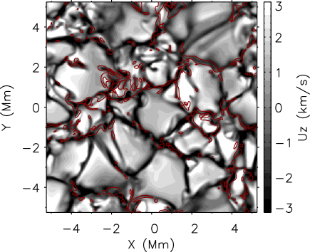
Figure 1: Left: The average vertical density (solid) and temperature (dashed) stratification. The dash-dotted line indicate the height where the density and temperature values ($1\times 10^{-7}$ g/cm³, 5730 K) are comparable with photospheric values.   Right: The vertical velocity structure at the photosphere ($z=$ -2.5 Mm). Red lines show regions with $|B_{z}|$ greater than 3G.

We then use this solution as the initial state of a 3-D simulation with a domain of dimensions of $10\times 10\times 15$ Mm³, which is comparable to the size of an ephemeral region on the sun. Within this superadiabatic background atmosphere, convective motion then can be initiated by breaking the symmetry with a small energy perturbation applied to the subsurface portion of the computational domain. In our simulations, we obtain solar-like convective structures with convective granules of upward velocity, up to 6 km/s, surrounded by narrow intergranular lanes of downward velocity up to 6 km/s, shown by the gray-scale image in the right panel of Figure 1. To build a magneto-convective state, we introduce a horizontal magnetic field, $B_{x}=1$ G, into the region below the surface, while other regions are initially field-free. The magnetic energy is less than $0.001\%$ of the kinetic energy of the turbulent motion, which dominates the dynamics in this case. Over time, the field is stretched and amplified by convective motions, and flux becomes concentrated in intergranular lanes, shown by red lines in the right panel of Figure 1, without noticeable deformation of the granular convection. Since the focus of this paper is not the study of the convective dynamo, we also experiment with stronger initial mean fields to more quickly build up semi-realistic models of magneto-convection.

We then put a $1$ G vertical magnetic field into the domain to heat the corona by activating the empirical coronal heating term $Q_{cr}$, and open the upper boundary to allow waves to travel outward. The vertical variation of the relaxed atmosphere is described in the left panel of Figure 1, which shows average density and temperature plotted as functions of height. At $z=-2.5$ Mm, the density and temperature values ($1\times 10^{-7}$ g/cm³, 5730 K) are comparable with the observed values of the photosphere, and thus, this layer is defined in our simulations as the solar surface.

After the generation of a realistic convective state and overlying atmosphere, we insert a thin, horizontal twisted flux rope into the model’s convection zone. Following Fan (2001) and Manchester et al. (2004), we describe the initial flux rope by

$${\bf B_{0}}=B_{0}e^{-r^{2}/a^{2}}\hat{\boldsymbol{x}}+qrB_{0}e^{-r^{2}/a^{2}}\hat{\boldsymbol{\theta}},$$ (9)

where we set $a=0.3$ Mm. q is the twisting factor defined as the angular rate of field line rotation per unit length in the axial direction. The density is depleted in the central section of the flux rope, which produces an $\Omega$-loop structure by buoyancy using:

$$\rho=\rho_{0}(1-\eta e^{-x^{2}/\lambda^{2}}),$$ (10)

where $\lambda=1.5$ Mm, and the ratio $\eta$ is defined as

$$\eta=\frac{\frac{1}{2}\left[B_{0}e^{-r^{2}/a^{2}}\right]^{2}\left[-1+\frac{1}{2}q^{2}(1-\frac{2r^{2}}{a^{2}})\right]}{p_{0}},$$ (11)

which maintains a force balance.

To make the total energy unchanged, we correct the pressure by:

$$p=p_{0}(1-\eta).$$ (12)

3 Results

Results from our model are presented as follows. In Section 3.1, we describe the steps we took to simulate the rise of a buoyant flux rope, and the structures that developed during the course of its ascent. In Section 3.2 we discuss the shearing motion during the emergence process, and finally in Section 3.3 analyzes a particular case of “U-loop” formation.

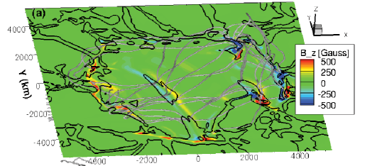
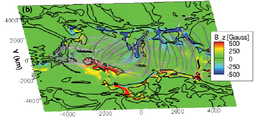
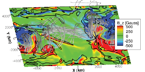
Figure 2: The 3-D structure of magnetic field of Run 1 (a), Run 2 (b) and Run 3 (c) at $t=20$, $20$, $16$ min, respectively. The planes show the $B_{z}$ on photosphere. Black lines outline regions with downflow speed greater than 1km/s. Flux ropes with more twist or strength have less horizontal expansion and more coherence during emergence.

3.1 Emergence of the Flux Rope

In the sections below, we experiment with different twisting and magnetic strength values shown in Table 1 and evaluate their role in affecting the emergence. At the photosphere, the flux rope first emerges as two closely-aligned flux concentrations with opposite polarities. Then these two polarities start to separate from each other since the buoyant section continues to lengthen. Figure 2 shows the 3-D structure of magnetic fields for each run, with the color showing the photospheric $B_{z}$ field, and black lines marking downdrafts with speed greater than 1 km/s. For Run 1, with a weak field $B_{0}=7.0$ kG and low twist $q=1.0$, we observe little coherency in the emerging flux rope, which expands preferentially in the horizontal direction. The horizontal expansion occurs 0.5 Mm above the photosphere, at the temperature minimum. And on the photosphere, convective motion dominates over the rising motion of magnetic flux, as seen in Panel (a) of Figure 2. The twisting factor was increased in Run 2, and a coherent flux rope was observed in the lower corona after emergence, shown in Panel (b). In Run 3, both twisting factor and flux rope strength are increased compared with Run 1. We find that the increase of a non-axial component of the initial magnetic field (Panel (c) of Figure 2) enhances coherency, and prevents the emerged rope from over-expansion in the horizontal direction, as shown in Panel (a). Turbulent plasma flows distort the flux rope during its rise, while a flux rope with strong magnetic field deforms the convective granules after emergence, consistent with Cheung et al. (2007). However, regardless of the deformation, the strong vertical magnetic fields concentrate in the downdrafts after fully emerging above the surface. In the following sections, we will analyze Run 3 in detail.

Table 1: Parameters for runs

runs	q	$B_{0}$ (kG)
1	-1.0	7.0
2	-1.5	7.0
3	-1.5	14.0

3.2 Shearing Motion

Figure 3: The evolution of sheared (solid) and emerged (dashed) energy flux at the photosphere for Run 2 (left) and Run 3 (right). In the right panel, dotted and dash-dotted lines show the evolution of shear and emerged fluxes, respectively, at $z=$ -0.45 Mm.

Photospheric shearing motions have long been observed to be in strong association with solar flares and CMEs (e.g., Meunier & Kosovichev 2003; Yang et al. 2004; Schrijver et al. 2005). Besides the photospheric motion, Athay et al. (1985) found a shearing area in the transition region and upper chromosphere. Helioseismic flow maps (Kosovichev & Duvall, 2006) also indicate the magnetic energy buildup prior to CMEs is driven by the strong shearing flows with speed 1-2 km/s at the depth of 4-6 Mm below the surface.

In our simulations, coherent shearing flows develop below the photosphere and extend into the lower corona in the later phase of emergence. We calculate the components of the Poynting flux associated with horizontal and vertical motions on the photosphere by:

$$E_{shear} = -\int\frac{1}{8\pi}\left(B_{x}u_{x}+B_{y}u_{y}\right)B_{z}dS,$$ (13)

$$E_{emerge} = \int\frac{1}{8\pi}\left(B_{x}^{2}+B_{y}^{2}\right)u_{z}dS.$$ (14)

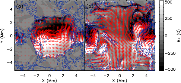
Figure 4: The vertical magnetic field structure on photosphere at times $t=$ 10 (a) and 15 (b) min for Run 3. Blue lines show regions with $|(\nabla\times{\bf u})_{z}|$ greater than 1.5 times of the average value. The horizontal magnetic field is shown by the red arrows. The locations of strong PILs show a good coincidence with regions with higher $|(\nabla\times{\bf u})_{z}|$ values.

The temporal evolution of the energy fluxes is shown in Figure 3. In Runs 2 and 3, the top of the flux rope reaches the photosphere at times $t=9.5$ and $5.5$ min, respectively, shown in Figure 3. When the magnetic field first emerges at the surface, a simultaneous increase in sheared and emerged energy flux occurs, with a greater increase in emerged flux. The emerging motion dominates the energy flux for the first 10 minutes, during which the buoyant part of the flux rope evolves to a fully emerged state. Afterwards, near the surface, the magnetic pressure gradient force is balanced by gravity and gas pressure, which slows down the emergence and decreases the emerged energy flux after the saturation of emergence. The emerged energy flux drops to negative values in the later phase due to the concentration and subduction of the magnetic field in downdrafts. Dotted and dash-dotted lines in right panel of Figure 3 show the shear and emerged energy fluxes, respectively, in lower corona, 2.05 Mm above the photosphere, which has a temporal delay of 6 min but represents a similar trend as the fluxes at the photosphere.

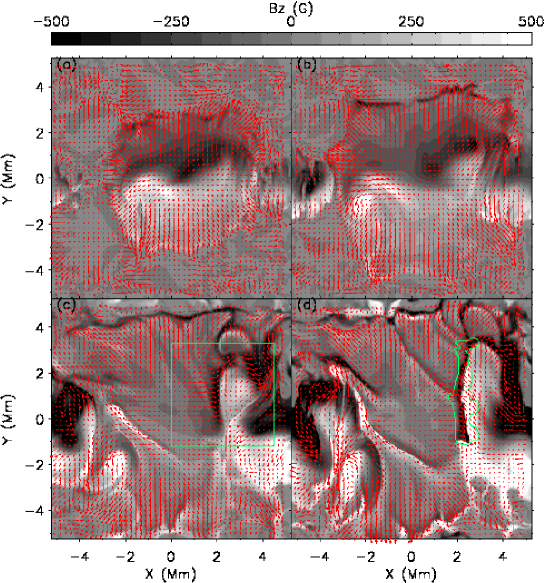
Figure 5: The vertical magnetic field structure on photosphere at times $t=$ 10 (a), 12 (b), 15 (c) and 20 (d) min for Run 3. The red arrows show the horizontal velocity field. In panel (d), the green line outlines the region with velocity shearing illustrated by $|(\nabla\times{\bf u})_{z}|$ greater than the average value. In panel (c), the green box marks the subregion shown in Figure 7 and Figure 9. High velocity shearing occurs along the PILs during the emergence.

When the rising motion succumbs to photospheric downflows, the main energy release into the overlying atmosphere is contributed by the shear flow, which continues long after the flux has emerged through the photosphere. The sheared energy flux increases by a factor of 4 from the initial emerging phase. The energy evolution resembles that shown in Manchester et al. (2004), with the fundamental difference that active convection ultimately subducts magnetic field and reverses the emerging energy flux.

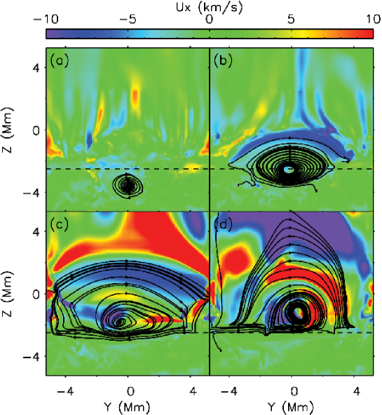
Figure 6: Variation of $u_{x}$ on $X=0$ plane at times $t=$ 5 (a), 10 (b), 15 (c) and 20 (d) min for Run 3. Black lines show the magnetic field lines on Y-Z plane, with arrows indicating the direction. Dashed lines indicate the height of the photosphere. Coherent shearing pattern develops in the lower corona and extends down to the chromosphere when the rope rises.

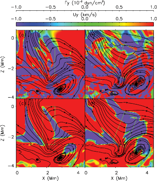
Figure 7: (a) $F_{y}$ structure at time $t=$ 16 min  (b) $F_{y}$ structure at time $t=$ 18 min  (c) $y$ component of velocity perpendicular to magnetic fields at time $t=$ 16 min  (d) $y$ component of velocity perpendicular to magnetic fields at time $t=$ 18 min in region marked by green box in Panel (c) of Figure 5 for Run 3. Black lines show the magnetic field lines on the plane, with arrows indicating the direction. Dashed lines show the height of the photosphere. The field lines form a U-loop structure with a shearing velocity up to $\pm$ 1.5 km/s on each side of the PIL (outlined by the green boxes).

Figure 4 shows the evolution of vertical and horizontal magnetic field structures at the photosphere for Run 3. The horizontal gradients in velocity are illustrated with contour lines of $(\nabla\times{\bf u})_{z}$. At $t=10$ min, Panel (a) of Figure 4 shows a highly sheared magnetic field structure at this initial phase. Panel (a) of Figure 5 shows a horizontal velocity field flowing outward from the center of the granule, at $t=10$ min, when the top of the flux rope reaches the photosphere and the size of the convective granule lying above it increases. After that, the emerging motion is saturated, and the fragmentations and distortions of the magnetic field mainly result from shearing and convective motions. In Panel (b) of Figure 5, the two polarities start to move along the PIL in opposite directions, and form strong PILs shown in Panel (c) and (d). At time $t=15$ min, Panel (b) of Figure 4 shows a good coincidence of the PIL and regions with $(\nabla\times{\bf u})_{z}$ greater than 1.5 times of the average value. This implies a high velocity shearing along the PIL at the photosphere in the later phase of emergence, which is clearly seen in the region outlined by the green box in Panel (d) of Figure 5.

Figure 6 shows the evolution of the horizontal velocity, $u_{x}$, and the magnetic field lines on the $X=0$ plane for Run 3. A coherent shearing pattern with velocity $u_{x}$ up to 20 km/s develops in the lower corona and extends down to the chromosphere and photosphere during the rising of the rope. The shear pattern is similar to Manchester et al. (2004) with notable exceptions of being more highly structured with reduced velocity. We also find that shear flows in the corona persist even when the convective motion washes out any coherent shearing at the photosphere.

3.3 U-loop Structure

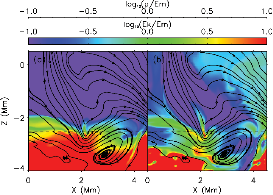
Figure 8: (a) Ratio of thermal pressure to magnetic energy $log_{10}(p/E_{mag})$ at time $t=$ 16 min  (b) ratio of kinetic energy to magnetic energy $log_{10}(E_{k}/E_{mag})$ at time $t=$ 16 min. Black lines show the magnetic field lines on the plane, with arrows indicating the direction. Dashed lines show the height of the photosphere. Kinetic and thermal energy dominate in the domain below the photosphere, while above it magnetic energy dominates.

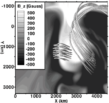
Figure 9: Bottom view of the magnetic field lines in region marked in green box in Panel (c) of Figure 5 for Run 3. Plane shows the $B_{z}$ structure on photosphere. The magnetic field lines run perpendicularly to the PIL, minimizing the energy.

Here, we examine a U-loop - a magnetic feature formed when magnetic flux is pulled down into an intergranular lane, as reported by Tortosa-Andreu & Moreno-Insertis (2009). We evaluate the role of Lorentz force ${\bf F}$ in a subregion outlined in Panel (c) of Figure 5 where the U-loop forms, by examining $F_{y}$ and the $y$ component of velocity perpendicular to the magnetic field $(u_{\perp})_{y}$. This velocity component, $(u_{\perp})_{y}$, excludes siphon flows parallel to the magnetic field and thus illustrates the motion of magnetic field lines. In Figure 7, we show that the field lines on the $X-Z$ plane evolve to a U-loop structure with a shearing velocity $(u_{\perp})_{y}$ up to $\pm$ 1.5 km/s on each side of the PIL (outlined by the green boxes). The upper two panels illustrate the magnitude of the Lorentz force while the bottom panels show the magnitude of $(u_{\perp})_{y}$. The fact that $F_{y}$ and $(u_{\perp})_{y}$ are in the same direction-reversing across the neutral line (outlined by the green boxes) suggests the velocity shearing is due to the Lorentz force. Panels (c) and (d) of Figure 5 show a highly sheared magnetic field and velocity field in this region on the photosphere. However, when viewed from the bottom, as shown in Figure 9 (with 3-D magnetic lines over a gray-scale image of the photospheric $B_{z}$ field in this region), the magnetic field lines are unsheared below the surface, running perpendicularly to the PIL, and minimizing the energy. Figure 8 shows the ratio of the thermal pressure and kinetic energy to the magnetic energy in the region in Figure 7. Below the photosphere, kinetic and thermal energy dominate, while above the photosphere, convective motion stops and gives way to the magnetic energy.

It has been commonly observed that the central regions of $\Omega$-loops become highly sheared as they emerge and unshear as they submerge (Manchester, 2007). We find for the first time that magnetic U-loops will unshear by flows driven by the Lorentz force, as illustrated by the gradient in $B_{y}$. These flows transport energy and axial flux from the convection zone to the corona, where the U-loop is expanding. This simulation further illustrates the dynamic coupling of the convection zone and corona, due to shearing flows driven by Lorentz force, suggested by Manchester (2007). This coupling occurs for two reasons: the transport of axial flux and the requirement that axial field strength be equilibrated along field lines to achieve a state of force balance.

4 Discussion and Conclusions

Observations have shown that CMEs originate from polarity inversion lines on the photosphere, where strong magnetic and velocity shearing occurs. Study of vector magnetograms of active regions (Falconer, 2001; Falconer et al., 2006) found the nonpotentiality of the magnetic fields, i.e. the total free magnetic energy, to be the determinant of the CME productivity. Other observations also indicate that solar eruptive events, e.g. flares, filaments, and prominences, preferentially occur in magnetic structures where the magnetic field runs parallel to the magnetic inversion line, i.e. highly sheared magnetic structures (Foukal, 1971; Leroy, 1989; Canfield et al., 1999; Liu et al., 2005; Su et al., 2007). Deng et al. (2006) observed persistent and long-lived ($>5$ hrs) shear flows in Active Region NOAA 10486 along the neutral line prior to the occurrence of the X10 flare on 2003 October 29, which may be explained by the successive emergence of a much larger and stronger flux rope/system than that in our simulations.

Surface plasma flows have long been recognized to have an important influence on the evolution of coronal magnetic fields. Many simulations, e.g. Mikic et al. (1988) and van der Holst et al. (2007), have been performed with flux ropes and arcades whose footpoints are subjected to surface motions imposed as boundary conditions. For example, Amari et al. (2003) has shown that converging motions toward the magnetic inversion line can drive a catastrophic nonequilibrium transition into eruptions when accompanied by shearing motions along the inversion line. In Antiochos et al. (1999), sheared arcades reconnect with a surrounding flux system, resulting in an eruption, in which the magnetic free energy stored in the closed shear arcade is released. In these coronal models, shear flows are only prescribed as boundary conditions to trigger instabilities and eruptions. Recent numerical simulations (Manchester, 2003; Manchester et al., 2004) have shown shear flows develop self-consistently during the emergence of the flux system (arcade and rope respectively) through a stratified atmosphere. The shearing motions result from the Lorentz force that occurs as the magnetic field expands into the stratified ambient atmosphere. This shearing mechanism explains the following: (1) coincidence of magnetic and velocity inversion lines; (2) the time evolution and magnitude of the shear flows in different layers of the atmosphere; (3) the large scale shear pattern, which is most concentrated at the PIL; (4) transport of flux and energy from the convection zone to the corona; (5) loss of equilibrium when the shear flows are unable to equilibrate the axial flux along magnetic field lines - a process that can explain many observed occurances of CMEs, eruptive filaments, and flares (Manchester, 2003; Manchester et al., 2004; Manchester, 2007, 2008; Archontis & Torok, 2008; MacTaggart & Hood, 2009). However, in these idealized models without the convective motion, shear flows grow rapidly in the absence of competing mechanism. In addition, the use of a purely adiabatic energy equation leads to expanding flux ropes whose plasma cools far too rapidly, thus inhibiting the emergence process.

In light of these problems, we incorporated additional physics into our MHD models, and simulated the buoyant rise of a twisted flux rope as it emerged through a turbulent model convection zone into a model corona. Flux ropes with more twist or greater magnetic strength can rise through the convection zone coherently, while less twisted or weaker flux ropes tend to expand in the horizontal direction, while being distorted by the turbulent motions, as shown by Figure 2. During its emergence, shearing motions at the photosphere develop and extend into the lower corona, with a speed up to 20 km/s, which is comparable with the shearing velocity of 20 km/s reported by Chae et al. (2000) in active region loops. In our simulations, shearing motion couples the emerged flux with the subsurface magnetic fields, and transfers the energy from below the surface into the solar atmosphere. In Run 3, where the twisting factor $q=-1.5$ and magnetic strength $B_{0}=14.0$ G, the total sheared energy can go up to $1.08\times 10^{30}$ ergs in 21 min, about $1\%$ of the average amount released in CMEs. The consistency between our results and previous simulations (Manchester et al., 2004) shows that the physical mechanism of Lorentz force-driven shear flows is very robust during the flux emergence in a domain comparable to ephemeral regions, regardless of the presence of thermodynamic processes such as turbulent convection. Given that active regions are 10 times (with 100 times the area) larger than this simulated flux concentration, our results suggest that shear flows driven by the Lorentz force can readily provide the free magnetic energy for CMEs.

In order to study the triggering mechanism for the explosive activities associated with magnetic field structures, we will extend our domain size to be comparable with the size of active regions and increase the flux rope size. Our model is very useful in the sense that it can be expanded in horizontal and vertical directions using the adaptive grids. The model includes different layers and physical processes in the solar atmosphere and new features can be easily implemented. In future simulations, we need to take into account the background magnetic field and the field-aligned heat conduction, and investigate the effects of surface footpoint motions on reconnection between emerging and ambient field, as reported by Archontis et al. (2004), Galsgaard et al. (2007), Archontis & Torok (2008) and MacTaggart & Hood (2009).

References

- Abbett et al. (2000) Abbett, W. P., Fisher, G. H., & Fan, Y. 2000, ApJ, 540, 548
- Abbett & Fisher (2003) Abbett, W. P., & Fisher, G. H. 2003, ApJ, 582, 475
- Abbett (2007) Abbett, W. P. 2007, ApJ, 665, 1469
- Amari et al. (2003) Amari, T., Luciani, J. F., Aly, J. J., Mikic, Z., & Linker, J. 2003, ApJ, 585, 1073
- Antiochos et al. (1999) Antiochos, S. K., DeVore, C. R., & Klimchuk, J. A. 1999, ApJ, 510, 485
- Archontis et al. (2004) Archontis, V., Moreno-Insertis, F., Galsgaard, K., Hood, A. & O’Shea, E. 2004, A&A, 426, 1047
- Archontis & Torok (2008) Archontis, V., & Torok, T. 2008, A&A, 492, L35
- Athay et al. (1985) Athay, R. G., Jones, H. P., & Zirin, H. 1985, ApJ, 288, 363
- Bercik (2002) Bercik, D. J. 2002, Ph.D. thesis, Michigan State University
- Caligari et al. (1995) Caligari, P., Moreno-Insertis, F., & Schüssler, M. 1995, ApJ, 441, 886
- Canfield et al. (1999) Canfield, R. C., Hudson, H. S., & McKenzie, D. E. 1999, Geophys. Res. Lett., 26, 627
- Cattaneo et al. (2003) Cattaneo, F., Emonet, T., & Weiss, N. 2003, ApJ, 588, 1183
- Chae et al. (2000) Chae, J. C., Wang, H., Qiu, J., Goode, P. R., & Wilhelm, K. 2000, ApJ, 533, 535
- Cheung et al. (2007) Cheung, M. C. M., Schüssler, M., & Moreno-Insertis, F. 2007, A&A, 467, 703
- Cheung et al. (2008) Cheung, M. C. M., Schüssler, M., Tarbell, T. D. & Title, A. M. 2008, ApJ, 687, 1373
- Deng et al. (2006) Deng, N., Xu, Y., Yang, G., Cao, W., Liu, C., Rimmele, T. R., Wang, H., & Denker, C. 2006, ApJ, 644, 1278
- Dere et al. (1997) Dere, K. P., Landi, E., Mason, H. E., Monsignori Fossi, B. C., & Young, P. R. 1997, A&AS, 125, 149
- Dere et al. (2009) Dere, K. P., Landi, E., Young, P. R., Del Zanna, G., Landini, M. & Mason, H. E. 2009, A&A, 498, 915
- Dorch & Nordlund (1998) Dorch, S. B. F., & Nordlund, A. 1998, A&A, 338, 329
- Emonet & Moreno-Insertis (1998) Emonet, T., & Moreno-Insertis, F. 1998, ApJ, 492, 804
- Fan et al. (1993) Fan, Y., Fisher, G. H., & Deluca, E. E. 1993, ApJ, 405, 390
- Fan (2001) Fan, Y. 2001, ApJ, 554, L111
- Fan (2008) Fan, Y. 2008, ApJ, 676, 680
- Fan (2009) Fan, Y. 2009, Living Rev. in Sol. Phys., 6,4
- Falconer (2001) Falconer, D. A. 2001, J. Geophys. Res., 106, 25185
- Falconer et al. (2006) Falconer, D. A., Moore, R. L., & Gary, G. A. 2006, ApJ, 644, 1258
- Fisher et al. (2000) Fisher, G. H., Fan, Y., Longscope, D. W., Linton, M. G. & Pevtsov, A. A. 2000, Sol. Phys., 192, 119
- Foukal (1971) Foukal, P. 1971, Sol. Phys., 19, 59
- Galsgaard et al. (2007) Galsgaard, K., Archontis, V., Moreno-Insertis, F. & Hood, A. W. 2007, ApJ, 666, 516
- Kosovichev & Duvall (2006) Kosovichev, A. G., & Duvall, T. L., 2006, Space Sci. Rev., 124, 1
- Leroy (1989) Leroy, J. L. 1989, in Dynamics and Structure of Quiescent Solar Prominences, ed. E. R. Priest, 150, 77
- Liu et al. (2005) Liu, C., Deng, N., Liu, Y., Falconer, D., Goode, P. R., Denker, C., & Wang, H. 2005, ApJ, 622, 722
- MacTaggart & Hood (2009) MacTaggart, D. & Hood, A. W. 2009, A&A, 508, 445
- Magara & Longcope (2003) Magara, T. & Longcope, D. W. 2003, ApJ, 586, 630
- Manchester & Low (2000) Manchester, IV, W. & Low, B. C. 2000, Phys. Plasmas, 7, 1263
- Manchester (2001) Manchester, IV, W. 2001, ApJ, 547, 503
- Manchester (2003) Manchester, IV, W. 2003, J. Geophys. Res., 108, 1162
- Manchester et al. (2004) Manchester, IV, W., Gombosi, T., DeZeeuw, D. & Fan, Y. 2004, ApJ, 610, 588
- Manchester (2007) Manchester, IV, W. 2007, ApJ, 666, 532
- Manchester (2008) Manchester IV, W. 2008, in Subsurface and Atmospheric Influences on Solar Activity, ASP Conference Proceedings, Eds. R. Howe, R. W. Komm, K. S. Balasubramaniam, & G. J. D. Petrie, 383, 91
- Martinez-Sykora et al. (2008) Martínez-Sykora, J., Hansteen, V., & Carlsson, M. 2008, ApJ, 679, 871
- Martinez-Sykora et al. (2009) Martínez-Sykora, J., Hansteen, V., DePontieu, B., & Carlsson, M. 2009, ApJ, 701, 1569
- Meunier & Kosovichev (2003) Meunier, N., & Kosovichev, A. 2003, A&A, 412, 541
- Mikic et al. (1988) Mikic, Z., Barnes, D. C., & Schnack, D. D. 1988, ApJ, 328, 830
- Nordlund et al. (1992) Nordlund, A., Brandenburg, A., Jennings, R. L., Rieutord, M., Ruokolainen, J., Stein, R. F., & Tuominen, I. 1992, ApJ, 392, 647
- Pevtsov et al. (2003) Pevtsov, A. A., Fisher, G. H., Acton, L. W., Longcope, D. W., Johns-Krull, C. M., Kankelborg, C. C., & Metcalf, T. R. 2003, ApJ, 598, 1387
- Powell et al. (1999) Powell, K. G., Roe, P. L., Linde, T. J., Gombosi, T. I., & DeZeeuw, D. L. 1999, J. Comput. Phys., 154, 284
- Rogers (2000) Rogers, F. J. 2000, Phys Plasmas, 7, 51
- Schrijver et al. (2005) Schrijver, C. J., DeRosa, M. L., Title, A. M., & Metcalf, T. R. 2005, ApJ, 628, 501
- Shibata et al. (1989) Shibata, K., Tajima, T., Steinolfson, R. S., & Matsumoto, R. 1989, ApJ, 345, 584
- Sokolov et al. (2008) Sokolov, I. V., Powell, K. G., Cohen, O., & Gombosi, T. I. 2008, in Numerical Modeling of Space Plasma Flows, ASP Conference Series, Eds. N. V. Pogorelov, E. Audit, & G. P. Zank, 385, 291
- Stein & Nordlund (2000) Stein, R. F. & Nordlund, A. 2000, Sol. Phys., 192, 91
- Su et al. (2007) Su, Y. , Golub, L., Van Ballegooijen, A. A. 2007, ApJ, 655, 606
- Tortosa-Andreu & Moreno-Insertis (2009) Tortosa-Andreu, A., & Moreno-Insertis, F. 2009, A&A, 507, 949
- van der Holst et al. (2007) van der Holst, B., Jacobs, C., & Poedts, S. 2007, ApJ, 671, L77
- Yang et al. (2004) Yang, G., Xu, Y., Cao, W., Wang, H., Denker, C., & Rimmele, T. R., 2004, ApJ, 617, L151