The Deep Water Abundance on Jupiter: New Constraints from Thermochemical Kinetics and Diffusion Modeling

Abstract

We have developed a one-dimensional thermochemical kinetics and diffusion model for Jupiter’s atmosphere that accurately describes the transition from the thermochemical regime in the deep troposphere (where chemical equilibrium is established) to the quenched regime in the upper troposphere (where chemical equilibrium is disrupted). The model is used to calculate chemical abundances of tropospheric constituents and to identify important chemical pathways for CO-CH₄ interconversion in hydrogen-dominated atmospheres. In particular, the observed mole fraction and chemical behavior of CO is used to indirectly constrain the Jovian water inventory. Our model can reproduce the observed tropospheric CO abundance provided that the water mole fraction lies in the range $(0.25-6.0)\times 10^{-3}$ in Jupiter’s deep troposphere, corresponding to an enrichment of 0.3 to 7.3 times the protosolar abundance (assumed to be H₂O/H${}_{2}=9.61\times 10^{-4}$). Our results suggest that Jupiter’s oxygen enrichment is roughly similar to that for carbon, nitrogen, and other heavy elements, and we conclude that formation scenarios that require very large ($>\,$8 times solar) enrichments in water can be ruled out. We also evaluate and refine the simple time-constant arguments currently used to predict the quenched CO abundance on Jupiter, other giant planets, and brown dwarfs.

1 Introduction

The water abundance in Jupiter’s deep atmosphere provides important clues for solar system formation and evolution and reveals conditions in the solar nebula at the time of giant-planet formation (e.g., Lunine et al., 2004). In addition, the planetary water inventory has important implications for the cloud structure, energy balance, thermal structure, and chemistry of the Jovian troposphere. Unfortunately, the deep water abundance is difficult to obtain by remote sensing methods because H₂O is expected to condense near the $\sim$5 bar level in Jupiter’s cold upper troposphere (e.g., see Taylor et al., 2004), and clouds and other opacity sources limit the depth to which infrared and other wavelength radiation can penetrate. The only in-situ measurement of the Jovian water abundance, by the Galileo Probe Mass Spectrometer (GPMS), pertains to a meteorologically anomalous “hot-spot” region characterized by low cloud opacity, low mixing ratios of condensable species, high thermal emission, and a water abundance which increased with depth (e.g., Orton et al., 1996, 1998; Niemann et al., 1998; Ragent et al., 1998; Sromovsky et al., 1998; Wong et al., 2004). Thus, it is unclear whether the probe descended deep enough to sample the well-mixed water abundance below the cloud base, and the Galileo probe value of H₂O/H${}_{2}=4.9\pm 1.6\times 10^{-4}$ at the 19-bar level (Wong et al., 2004) is generally considered to be a lower limit for Jupiter’s O/H inventory (e.g., Roos-Serote et al., 2004; Taylor et al., 2004; Wong et al., 2004; de Pater et al., 2005). For this reason, chemical models must be used to determine the deep water abundance in Jupiter’s atmosphere until further measurements become available, such as microwave observations from the Juno mission or future deep-atmosphere probes (e.g., Bolton et al., 2006; Atreya, 2004).

Several investigators have used clever methods to estimate the deep H₂O abundance of the giant planets by considering the observed tropospheric abundance of CO and other trace constituents and by investigating how H₂O chemistry and atmospheric transport can influence the abundance of these trace species (e.g., Prinn and Barshay, 1977; Fegley and Prinn, 1985, 1988; Lodders and Fegley, 1994, 2002; Bézard et al., 2002; Visscher and Fegley, 2005). However, Prinn and Barshay (1977), and all subsequent modelers who used their kinetic schemes, were limited by a lack of key chemical kinetics data, and some of the initial kinetic assumptions have been shown to be incorrect (Dean and Westmoreland, 1987; Yung et al., 1988; Griffith and Yelle, 1999; Bézard et al., 2002; Cooper and Showman, 2006). In addition, some of the transport time-scale arguments in the earlier works have been shown to have inappropriate assumptions (Smith, 1998; Bézard et al., 2002). These problems offset each other to an extent, such that models using earlier assumptions yield reasonable results (cf. Visscher and Fegley, 2005; Bézard et al., 2002). Fegley and Prinn (1988) found that H₂O/H${}_{2}=(0.46-5.8)\times 10^{-3}$ is consistent with CO kinetics and atmospheric mixing on Jupiter, whereas Bézard et al. (2002) derived H₂O/H${}_{2}=(0.34-15.3)\times 10^{-3}$ using revised kinetic and transport time-scale parameters (Page et al., 1989; Yung et al., 1988; Smith, 1998) and improved CO observations. Further refinement of this estimate was not possible in the Bézard et al. analysis due to uncertainties in reaction kinetics, convective mixing rates, and the back-of-the-envelope time-scale arguments used to derive the H₂O abundance.

Here we attempt to improve the determination of the deep water abundance in Jupiter’s atmosphere by taking advantage of recent updates in thermodynamic parameters and reaction rate coefficients and by using a numerical model to provide a more rigorous quantitative test of the simple kinetic vs. transport time-scale approach. With a numerical model, we implicitly solve the continuity equations for all tropospheric constituents, considering reaction kinetics and atmospheric transport. As a result, our model tracks the transition from the thermochemical regime in the deep troposphere (where chemical equilibrium is established), to a quenched regime in the upper troposphere (where chemical equilibrium is disrupted). In contrast to previous studies, we make no a priori selection of the reaction mechanism, nor of the rate-determining step for the chemical conversion of CO into CH₄. Instead, we input a full suite of chemical kinetic reactions connecting the different relevant tropospheric species, and allow the dominant chemical pathways for the conversion of CO$\rightarrow$CH₄ to be identified from our model results. Furthermore, we make no assumptions about the mixing length scale but instead model atmospheric transport via diffusion for an assumed eddy diffusion coefficient profile. We explore the effects of the tropospheric water abundance on the chemical behavior of CO and other oxidized carbon gases and use the observed CO abundance to indirectly constrain the water inventory in Jupiter’s deep atmosphere.

The paper is organized as follows. We begin with a description of our chemical model and the CO chemical constraint in §2. We present our model results in §3, derive an estimate of Jupiter’s deep water abundance using CO as an observational constraint, identify the dominant chemical pathways involved for CO$\rightarrow$CH₄ conversion in Jupiter’s troposphere, and discuss the chemical behavior of other oxygen-bearing carbon species. In §4 we discuss implications of our results for constraining Jupiter’s total oxygen inventory and planetary formation scenarios, and conclude with a summary in §5.

2 Chemical Model

2.1 Numerical Approach

We use the Caltech/JPL KINETICS code (Allen et al., 1981) to calculate the vertical distribution of atmospheric constituents in Jupiter’s troposphere by solving the coupled one-dimensional continuity equations as a function of time $t$ and altitude $z$ for each species:

$$\frac{\partial n_{i}}{\partial t}+\frac{\partial\Phi_{i}}{\partial z}=P_{i}-L_{i},$$ (1)

where $n_{i}$ is the number density (cm^-3), $\Phi_{i}$ is the vertical flux (molecules cm^-2 s^-1), $P_{i}$ is the chemical production rate (molecules cm^-3 s^-1), and $L_{i}$ is the chemical loss rate (molecules cm^-3 s^-1) of species $i$.

The continuity equations are solved using finite-difference techniques for 144 atmospheric levels, with a vertical resolution of at least twenty altitude levels per scale height. Jupiter’s pressure-temperature profile is taken from Galileo entry probe data (Seiff et al., 1998) from 17 bar to the 22 bar, 427.7 K level (i.e., the maximum depth achieved by the probe before its destruction) and is extended to greater temperatures and pressures along an adiabat using the method described by Fegley and Prinn (1985). A zero flux boundary condition is maintained at the top (17.4 bar, 399 K) and bottom (12,650 bar, 2500 K) of the model, with thermochemical equilibrium being used to define the initial conditions. The relative abundances of the elements are thus defined a priori, and no mass enters or leaves the system. Although our model does not include rock-forming elements which may react with oxygen in Jupiter’s deep atmosphere, we do consider the partial removal of oxygen into rock (see §2.3 below) based upon the approach of Lodders (2004) and Visscher and Fegley (2005) so that our abundance calculations involving oxygen are correct for higher altitudes ($T<2000$ K; cf. Fig. 39 in Fegley and Lodders, 1994). Model calculations are performed until successive iterations differ by no more than 0.1%.

2.2 Eddy Diffusion Coefficient

In the context of our one-dimensional model, transport is assumed to occur by eddy diffusion, characterized by a vertical eddy diffusion coefficient $K_{zz}$. In the absence of a strong magnetic field or rapid rotation, the eddy diffusion coefficient can be estimated from free-convection and mixing-length theories (Stone, 1976; Gierasch and Conrath, 1985), using the scaling relationship

$$K_{zz}\approx wH\approx\left(\frac{Fk_{\textrm{B}}}{\rho mc_{p}}\right)^{1/3}H$$ (2)

where $w$ is the characteristic vertical velocity over which convection operates (cm s^-1), $F$ is Jupiter’s internal heat flux (5.44 W m^-2, Hanel et al., 1981; Pearl and Conrath, 1991), $k_{\textrm{B}}$ is the Boltzmann constant, $\rho$ is the atmospheric mass density (g cm^-3), $m$ is the atmospheric mean molecular mass (g), and $c_{p}$ is the atmospheric specific heat at constant pressure (erg K^-1 g^-1). The characteristic length scale over which mixing operates is assumed to be the atmospheric pressure scale height $H$, given by

$$H=\frac{k_{\textrm{B}}T}{mg}$$ (3)

where $g$ is the gravitational acceleration. Eq. (2) yields $K_{zz}\sim 7\times 10^{8}$ cm² s^-1 throughout much of Jupiter’s deep troposphere.

However, strong magnetic fields or rapid rotation can affect convection and alter $K_{zz}$ (e.g., Flasar and Gierasch, 1977; Stevenson, 1979; Fernando et al., 1991). Rotation reduces $K_{zz}$, whereas magnetic fields can either increase or decrease $K_{zz}$ over the estimates from standard mixing-length theory (Stevenson, 1979). Considering rotation alone, we use the equations developed by Flasar and Gierasch (1977, 1978) to describe small-scale thermally driven convection in a rapidly rotating atmosphere. As outlined by these authors, the characteristic vertical velocity $w$ for turbulent convection under these conditions is

$$w\ \approx \ \left(-\alpha gS\right)^{1/2}\,H^{2}, \quad{\rm for}\ Ro\gg|\sin\lambda|$$ (4)

$$w\ \approx \ \left(\frac{Ro}{\sin\lambda}\right)^{2}\left(-\alpha gS\right)^{1/2}\,H^{2}, \quad{\rm for}\ Ro\ll|\sin\lambda|$$ (5)

where $\alpha$ is the thermal expansion coefficient ($=1/T$ for an ideal gas), $S$ is the static stability $\partial\theta/\partial r$ (K cm^-1), i.e., the radial gradient of the potential temperature $\theta$ (and note that $S<0$ for free convection, as we are assuming here), $\lambda$ is the planetocentric latitude, and $Ro$ is the Rossby number associated with the convective flow:

$$Ro=\frac{(-\alpha gS)^{1/2}}{2\Omega}$$ (6)

where $\Omega$ is the rotational angular velocity (s^-1). Note that Eq. (4), which is valid for near-equatorial latitudes, is the same expression that is derived from mixing-length theory in non-rotating systems (see Eq. (2) above). At non-equatorial latitudes, Eq. (5) is appropriate, although it is convenient to replace $S$ with an expression involving $F$, the internal heat flux — a measured quantity. From mixing-length theory,

$$w\approx\frac{-F}{\rho c_{p}HS}.$$ (7)

After equating Eq. (5) and Eq. (7) and solving for $S$ and $Ro$ in terms of $F$, we find that

$$K_{zz}\approx\left[\frac{{k_{\textrm{B}}}FH^{1/3}}{\rho mc_{p}(4\Omega^{2}\sin^{2}\lambda)^{2/3}}\right]^{3/5}\quad\quad{\rm for}\ Ro\ll|\sin\lambda|$$ (8)

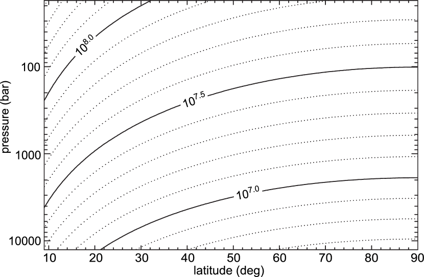
Figure 1: Eddy diffusion coefficient $K_{zz}$ at non-equatorial latitudes as a function of latitude and pressure predicted using the theory of Flasar and Gierasch (1977, 1978) for thermally driven turbulent convection in a rapidly rotating system (see Eq. (8)).

Figure 1 shows the solution to Eq. (8) for non-equatorial latitudes over our model pressure range, although we should note that the condition $Ro\ll|\sin\lambda|$ begins to break down at high altitudes and low latitudes (e.g., $Ro=|\sin\lambda|$ for 20 bar at 3^∘ latitude). Note that these $K_{zz}$ values are smaller than those predicted by standard mixing-length theory in a non-rotating atmosphere (see above); moreover, there is a very strong latitude dependence of $K_{zz}$ at any particular pressure. As noted by Flasar and Gierasch (1977), such meridional variations in $K_{zz}$ could have some interesting consequences, including the production of meridional gradients in temperature and in the mixing ratios of quenched disequilibrium species like CO. However, these gradients may in turn drive meridional fluxes that act to homogenize the temperatures and abundances. It is therefore difficult to determine an appropriate $K_{zz}$ profile to adopt for our models.

The Galileo probe entered the Jovian atmosphere in the Northern Equatorial Belt (NEB) near 6.5^∘ N latitude, and the CO observations of (Bézard et al., 2002) were also centered in the NEB near 9^∘ N latitude. At 9^∘ latitude, Eq. (8) implies $K_{zz}$ $\sim$ 4$\,\times\,10^{7}$ cm² s^-1 at 2400 bar, increasing to 1$\,\times\,10^{8}$ cm² s^-1 at 250 bar and 2.5$\,\times\,10^{8}$ cm² s^-1 at 20 bar. Because of uncertainties in the appropriate values of $K_{zz}$ in Jupiter’s deep troposphere, we adopt an altitude-independent $K_{zz}$ value of $1\times 10^{8}$ cm² s^-1 for our nominal model, but we also explore the effects of a range of altitude-independent $K_{zz}$ values from $4\times 10^{7}$ to $1\times 10^{9}$ cm² s^-1, as well as consider $K_{zz}$ values that vary with altitude using Eq. (8). We assume that this range encompasses all plausible values for $K_{zz}$ near the quench level.

2.3 Atmospheric Composition

Our model includes 108 hydrogen, carbon, nitrogen, oxygen, and phosphorus species that are subject to vertical transport and chemical production and loss. The measured relative abundances of these elements (see Table 1) are used to define our initial conditions. The observed abundances of sulfur (as H₂S) and the noble gases Ar, Kr, and Xe are shown in Table 1 for comparison. Atmospheric mixing ratios for He, CH₄ and NH₃ are taken from GPMS and helium interferometer measurements: He/H${}_{2}=0.1574$ (von Zahn et al., 1998; Niemann et al., 1998), and CH₄/H${}_{2}=2.37\times 10^{-3}$ and NH₃/H${}_{2}=6.64\times 10^{-4}$ (Wong et al., 2004). Our adopted phosphorus elemental abundance is based on a deep phosphine mixing ratio of PH₃/H${}_{2}=8\times 10^{-7}$ derived from Voyager IRIS (Kunde et al., 1982; Lellouch et al., 1989), Galileo NIMS (Irwin et al., 1998), Kuiper Airborne Observatory (Bjoraker et al., 1986) and ground-based (Bézard et al., 2002) 5-$\mu$m observations of Jupiter.

The Galileo entry probe measured a tropospheric water abundance of H₂O/H${}_{2}=4.9\times 10^{-4}$ near the 19-bar level (Wong et al., 2004), which corresponds to a subsolar O/H ratio. As was previously mentioned, it is unclear whether this value is representative of Jupiter’s deep, well-mixed water inventory because the probe entered a meteorologically dry hot-spot region and because the H₂O abundance increased nearly tenfold over the previous measurement at the 11-bar level (see Wong et al., 2004). Subsolar O/H values are also consistent with 5-$\mu$m observations from the Kuiper Airborne Observatory (KAO) (Larson et al., 1975; Bjoraker et al., 1986), the Voyager Infrared Interferometer Spectrometer (IRIS) (Drossart and Encrenaz, 1982; Kunde et al., 1982; Bjoraker et al., 1986; Lellouch et al., 1989), the Galileo Near-Infrared Mapping Spectrometer (NIMS) (Irwin et al., 1998; Roos-Serote et al., 1998), and the Infrared Space Observatory (ISO) (Encrenaz et al., 1996; Roos-Serote et al., 1999, 2004). However, the interpretation of the observations is complicated by several factors: (1) these 5-$\mu$m observations are weighted by thermal emission from the relatively dry and cloud-free hot-spot regions, (2) the observations are most sensitive to an altitude region in which water is expected to condense so that the H₂O mole fraction will be varying strongly with altitude, and (3) the results are highly dependent on assumptions regarding cloud structure and extinction. As is discussed by Roos-Serote et al. (2004), the Galileo NIMS observations are consistent overall with a deep O/H ratio of 1-2 times solar (see the discussion below on the solar ratio) and Roos-Serote et al. (2004) state that “subsolar values of the O/H ratio cannot be reconciled with the analyzed data,” but this conclusion is also model dependent. Due to the difficulties in determining the O/H ratio from remote-sensing observations and due to the ambiguities in interpreting whether the probe data are representative of the whole planet, we treat the oxygen elemental abundance as a free parameter in our model — indeed, the main free parameter that we are ultimately trying to constrain from our model-data comparisons — and we consider a wide range of H₂O/H₂ ratios in order to explore the effect of this parameter on tropospheric chemistry and the CO abundance.

Table 1 also contains the elemental enrichment factors relative to the assumed protosolar abundances. Elemental abundances for the solar nebula (i.e., protosolar abundances) are taken from Lodders et al. (2009). These abundances are slightly different from present-day solar photospheric abundances because of gravitational settling of heavy elements in the Sun (Lodders, 2003) and represent the bulk elemental composition of the Sun and solar nebula. As in previous studies (Lodders, 2004; Visscher and Fegley, 2005), the protosolar H₂O/H₂ ratio is defined by taking the total oxygen abundance ($\Sigma$O/H${}_{2}=1.21\times 10^{-3}$) and subtracting the portion that forms rock (O${}_{\textrm{rock}}$):

$$\textrm{O}_{\textrm{H}_{2}\textrm{O}}=\Sigma\textrm{O}-\textrm{O}_{\textrm{rock}}.$$ (9)

In a gas with a protosolar composition (Lodders et al., 2009), the formation of rock effectively removes $\sim$20% of the total oxygen inventory. Throughout the following, we thus define the water enrichment factor ($E_{\textrm{H}_{2}\textrm{O}}$) as

$$E_{\textrm{H}_{2}\textrm{O}}=(\textrm{H}_{2}\textrm{O}/\textrm{H}_{2})_{\textrm{Jupiter}}/(\textrm{H}_{2}\textrm{O}/\textrm{H}_{2})_{\textrm{solar}},$$ (10)

in which enrichments over “solar” refer to a protosolar abundance of H₂O/H₂ $=9.61\times 10^{-4}$. Using this definition, the Galileo probe measured a water abundance equivalent to 0.51x solar ($E_{\textrm{H}_{2}\textrm{O}}=0.51$) in Jupiter’s troposphere.

The relative abundance of H₂ (which comprises $86\%$ of the atmosphere) is calculated by difference using the observed mole fractions for He, CH₄, NH₃, PH₃, and varying assumptions for the H₂O mole fraction. From the adopted abundances of these major compounds, the initial chemical composition for all 108 species in the model is calculated along Jupiter’s pressure-temperature profile by thermochemical equilibrium. We use the NASA CEA (Chemical Equilibrium with Applications) code (Gordon and McBride, 1994) for our equilibrium calculations, utilizing thermodynamic parameters from the compilations of Gurvich et al. (1989, 1991, 1994); Chase (1998); Burcat and Ruscic (2005) and other literature sources. Figure 2 shows our equilibrium results for carbon chemistry in Jupiter’s atmosphere, which are similar to the results of Fegley and Lodders (1994, see their Fig. 17) with the exception of H₂CO and CH₂: here we use the H₂CO enthalpy of formation from Gurvich et al. (1989, 1991, 1994) instead of Chase (1998) based upon the recommendation of da Silva et al. (2006), and we calculate the mole fraction abundances of ¹CH₂ and ³CH₂ individually using updated thermodynamic parameters from Ruscic et al. (2005). From this initial equilibrium condition, we run the kinetic-transport model to solve the continuity equations (described by Eq. 1) until steady state is achieved.

2.4 Chemical Reactions

Approximately 1800 chemical reactions are included in our model. Photolysis reactions are omitted because the tropospheric pressure levels under consideration ($\geq 17$ bars) are too deep for ultraviolet photons to penetrate. Our reaction list is based upon previous chemical models of giant-planet atmospheres (e.g., Gladstone et al., 1996; Moses et al., 1995a, b, 2000a, 2000b, 2005) and includes numerous rate coefficient updates from combustion chemistry studies over the past two decades (e.g., Baulch et al., 1992, 1994, 2005; Smith et al., 1999; Dean and Bozzelli, 2000; Korobeinichev et al., 2000; Gardiner, 2000; Miller et al., 2005).

All of the reactions in the model are reversed using the principle of microscopic reversibility,

$$K_{eq}=\frac{k_{f}}{k_{r}},$$ (11)

where $K_{eq}$ is the equilibrium constant, $k_{f}$ is the rate coefficient for the forward reaction, and $k_{r}$ is the rate coefficient for the reverse reaction. The thermodynamic parameters for calculating $K_{eq}$ are taken primarily from the compilations of Gurvich et al. (1989, 1991, 1994), Chase (1998), and Burcat and Ruscic (2005). We also adopt updated thermodynamic data for several radical species (notably OH, CH₃, CH₂OH and CH₃O) from Ruscic et al. (2002, 2005). Equation (11) is used to determine $k_{r}$ for every reaction at each of the 144 atmospheric levels using the appropriate temperature-dependent values for $k_{f}$ and $K_{eq}$. The outcome of this procedure is a reaction list which consists of $\sim$900 forward reactions and $\sim$900 complimentary reverse reactions, which can be used to accurately reproduce equilibrium abundances based upon the selected thermodynamic parameters. In other words, in the absence of disequilibrium effects such as photochemistry or atmospheric mixing, and given sufficient time to reach a steady state, our kinetic model results are indistinguishable from those given by Gibbs energy minimization or mass-action, mass-balance thermodynamic-equilibrium calculations.

For three-body (termolecular) reactions, we assume that the forward reaction rate constant $k_{f}$ (cm⁶ s^-1) obeys the expression

$$k_{f}=\left(\frac{k_{0}}{1+\frac{k_{0}[\textrm{M}]}{k_{\infty}}}\right)F_{c}^{\beta},$$ (12)

where $k_{0}$ is the low-pressure three-body limiting value (cm⁶ s^-1), $k_{\infty}$ is the high-pressure limiting value (cm³ s^-1), and $[\textrm{M}]$ is the total atmospheric number density (cm^-3). The exponent $\beta$ in Eq. (12) is given by

$$\beta=\left(\frac{1}{1+\left[\log_{10}\left(\frac{k_{0}[\textrm{M}]}{k_{\infty}}\right)\right]^{2}}\right),$$ (13)

and we assume $F_{c}\approx 0.6$ (DeMore et al., 1992) except where specified in Moses et al. (2005). Termolecular and unimolecular reactions in the model are also reversed using the method described above (Eq. (11)).

2.5 CO Chemical Constraint

Carbon monoxide was first detected on Jupiter by Beer (1975) in the 5-$\mu$m window, with follow-up observations by Beer and Taylor (1978), Larson et al. (1978), and Noll et al. (1988, 1997). High-spectral-resolution observations that resolve the line shapes are needed to determine the origin of the CO, which can have either an internal source (i.e., from rapid mixing from the deep troposphere) or an external source (e.g., from satellite or meteoroidal debris). We are concerned solely with the internal source in this paper. As such, we rely on the observations that have most definitively resolved the CO vertical profile, those of Bézard et al. (2002). From ground-based $\sim$4.7 $\mu$m observations with a very high spectral resolution of 0.045 cm^-1, Bézard et al. (2002) determined that both internal and external sources contribute to CO on Jupiter and concluded that the derived tropospheric mole fraction of $(1.0\pm 0.2)\times 10^{-9}$ represents the contribution from the internal source.

Our basic approach for constraining Jupiter’s water inventory is similar to the method adopted by previous authors (e.g., Fegley and Prinn, 1988; Fegley and Lodders, 1994; Lodders and Fegley, 1994; Bézard et al., 2002; Visscher and Fegley, 2005): the observed abundance and chemical behavior of CO is used to estimate the H₂O abundance in Jupiter’s atmosphere. Deep in the troposphere, CO is produced from water and methane via the net thermochemical reaction

$$\textrm{CH}_{4}+\textrm{H}_{2}\textrm{O}=\textrm{CO}+3\textrm{H}_{2}\quad,$$ (14)

At high pressures and low temperatures, the reactants on the left-hand side of the reaction (CH₄, H₂O) are favored, whereas CO becomes more stable at low pressures and high temperatures. On Jupiter, the temperature factor is more important, and the CO abundance is expected to increase with depth, although methane remains the dominant carbon-bearing gas throughout the atmosphere. The equilibrium constant expression for reaction (14) may be written as

$$K_{\ref{r: CO net thermochemical reaction}}=\frac{[\textrm{CO}][\textrm{H}_{2}]^{3}}{[\textrm{CH}_{4}][\textrm{H}_{2}\textrm{O}]},$$ (15)

where $K_{\ref{r: CO net thermochemical reaction}}$ is the equilibrium constant for reaction (14) and $[i]$ is the concentration (cm^-3) of each species $i$. Rearranging this expression,

$$[\textrm{CO}]=K_{\ref{r: CO net thermochemical reaction}}[\textrm{CH}_{4}][\textrm{H}_{2}\textrm{O}]/[\textrm{H}_{2}]^{3},$$ (16)

shows that [CO]$\,\propto\,$[H₂O] at equilibrium for constant pressure and temperature conditions (e.g., Fegley and Prinn, 1988; Visscher and Fegley, 2005). Thus, if thermochemical equilibrium holds, the abundance of any one of these species in reaction (14) at a given altitude (i.e., at a given pressure and temperature) can be readily calculated from the observed abundances of the other three species at the same altitude in Jupiter’s atmosphere.

However, the observed CO mole fraction of $X_{\textrm{CO}}=(1.0\pm 0.2)\times 10^{-9}$, reported by Bézard et al. (2002) for the 6-bar level in Jupiter’s atmosphere, is many orders of magnitude higher than the CO abundance predicted under thermochemical equilibrium conditions for any plausible assumption about the deep water abundance on Jupiter and provides clear evidence of disequilibrium processes at work in the troposphere (e.g., Prinn and Barshay, 1977; Barshay and Lewis, 1978; Fegley and Prinn, 1985, 1988; Fegley and Lodders, 1994; Bézard et al., 2002). Carbon monoxide is not in equilibrium in Jupiter’s upper troposphere, and therefore Eq. (16) cannot be used to derive Jupiter’s deep water inventory.

Prinn and Barshay (1977) demonstrated that the observed CO abundance likely results from mixing from deeper atmospheric levels where CO is more abundant. As parcels of gas rise in Jupiter’s atmosphere, CO is destroyed by conversion into CH₄ at a rate that falls off dramatically with decreasing temperatures. The observable amount of CO in the upper atmosphere thus depends upon the relative time scales of CO destruction kinetics (characterized by $t_{chem}$) and convective vertical mixing (characterized by $t_{mix}$) (e.g., see Prinn and Barshay, 1977; Fegley and Prinn, 1985). Deep in the troposphere, $t_{chem}<t_{mix}$ and thermochemical equilibrium is achieved because kinetic reactions dominate over atmospheric mixing. At higher, colder altitudes, $t_{chem}>t_{mix}$, and disequilibrium prevails because vertical mixing operates faster than reaction kinetics can attain equilibrium. At some intermediate “quench” level defined by $t_{chem}=t_{mix}$, the CO mole fraction becomes quenched; above this level, the CO abundance remains fixed at the equilibrium mole fraction achieved at the quench level (Prinn and Barshay, 1977). As a result, the observed CO mole fraction in Jupiter’s upper atmosphere still serves as useful chemical probe for conditions in Jupiter’s deep atmosphere (e.g., Fegley and Prinn, 1983; Fegley and Lodders, 1994; Bézard et al., 2002), despite the departure from equilibrium, provided that the kinetics of the CO $\rightarrow$ CH₄ conversion process is accurately known (to define $t_{chem}$) and the rate of atmospheric mixing can be constrained (to define $t_{mix}$).

Although we go beyond the back-of-the-envelope $t_{chem}$-$t_{mix}$ approach with our kinetic-transport model, the underlying principle is the same. We determine the range of water enrichments that are consistent with the observed CO mole fraction for different plausible assumptions of the eddy diffusion coefficient and thereby indirectly constrain Jupiter’s global water inventory.

3 Model Results

3.1 CO Profiles and Their Sensitivity to Model Free Parameters

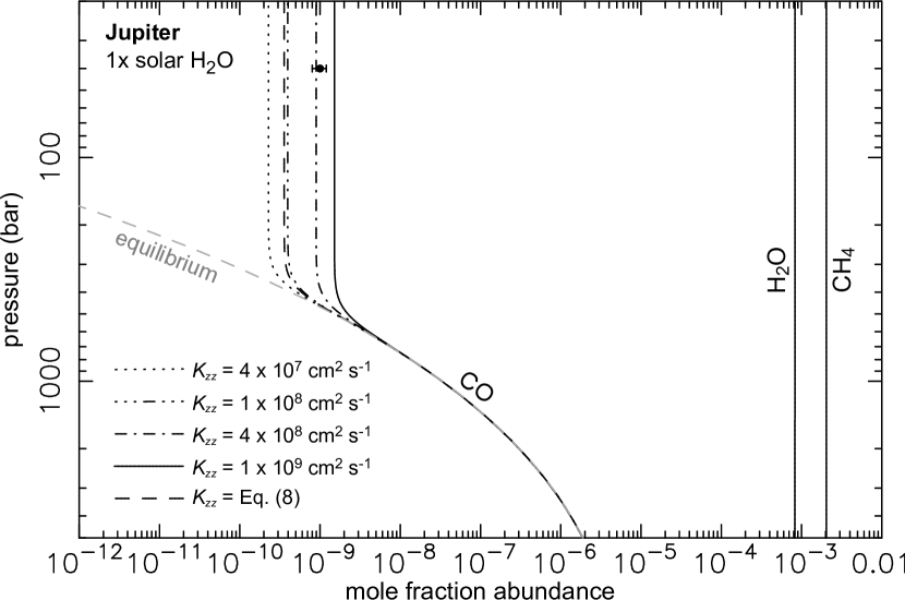
Figure 3: Vertical profiles for the CO, H₂O, and CH₄ mole fractions in Jupiter’s atmosphere for an assumed water enrichment of 1x solar (where we assume the solar value is H₂O/H${}_{2}=9.61\times 10^{-4}$, Lodders (2004); Lodders et al. (2009) and for assumed constant $K_{zz}$ values of $4\times 10^{7}$ (dotted line), $1\times 10^{8}$ (dot-dot-dot-dash line), $4\times 10^{8}$ (dash-dot line), and $1\times 10^{9}$ cm² s^-1 (solid line), as well as a $K_{zz}$ profile determined by Eq. (8) (dashed black line). The dashed gray line represents the CO abundance predicted by chemical equilibrium using the NASA CEA code. The circle with error bars represents the observed tropospheric CO mole fraction reported by Bézard et al. (2002). Note that if the deep water enrichment is 1x solar, as in the models shown here, the CO observations are best reproduced for $K_{zz}$ = $4\times 10^{8}$ cm² s^-1. Note also that water and methane are the dominant oxygen- and carbon-bearing gases, respectively, throughout Jupiter’s deep troposphere.

The CO vertical profiles resulting from our thermochemical kinetics and diffusion model are presented in Fig. 3 for various assumptions about the eddy diffusion coefficient and for a single assumption about the deep water abundance (1x solar). Shown for comparison is the observed CO mole fraction of $X_{\textrm{CO}}=(1.0\pm 0.2)\times 10^{-9}$ reported by Bézard et al. (2002) for the 6-bar level on Jupiter; note that we have assumed that this value remains constant down to at least the few tens of bar region. The dashed gray line in Fig. 3 shows the predicted equilibrium abundance of CO (calculated using the NASA CEA code), which increases with depth. In the deep atmosphere ($P\gtrsim 600$ bars, $T\gtrsim 1100$ K), the modeled CO abundance follows thermochemical equilibrium because the energy barriers for chemical reactions are easily overcome at these higher temperatures. As a result, the characteristic chemical time scale for interconversion between CO and CH₄ is much shorter than the time scale for vertical mixing ($t_{chem}\ll t_{mix}$), and equilibrium is readily achieved. However, as atmospheric parcels are transported to higher, colder altitudes, the chemical kinetic timescale becomes longer (i.e., the reactions become slower) relative to the mixing time scale, and the CO mole fraction can become quenched. In Fig. 3, divergence from the equilibrium profile occurs where vertical convective mixing begins to drive the CO abundance out of equilibrium and toward a constant quenched mole fraction. The transition region between the equilibrium and quenched regimes (where $t_{chem}\approx t_{mix}$) is not abrupt but occurs over a range of altitudes approximately equal to one pressure scale height: for example, at $K_{zz}=1\times 10^{8}$ cm² s^-1, the modeled CO abundance diverges from equilibrium near the $640$-bar level and resumes a constant quenched profile above the $200$-bar level. Our numerical models confirm the analytic prediction of Prinn and Barshay (1977) that the CO mole fraction remains fixed at altitudes above the quench region when the chemical reaction kinetics for CO$\,\rightarrow\,$CH₄ are extremely slow relative to the rate of vertical mixing ($t_{chem}\gg t_{mix}$).

Figure 3 illustrates that the “quenched” upper tropospheric CO mole fraction depends on the strength of convective mixing. For stronger convective mixing (i.e., larger $K_{zz}$), CO is quenched deeper in the atmosphere where the CO mole fraction is larger. Conversely, weaker mixing results in lower quenched CO mole fractions. If the deep water enrichment is 1x solar, Fig. 3 shows that the CO observations are best reproduced for $K_{zz}$ = $4\times 10^{8}$ cm² s^-1, if we assume a constant $K_{zz}$ profile with altitude. If the $K_{zz}$ profile varies with altitude, as with the model represented by a black dashed line in Fig. 3, the results are controlled by the $K_{zz}$ value near the quench level.

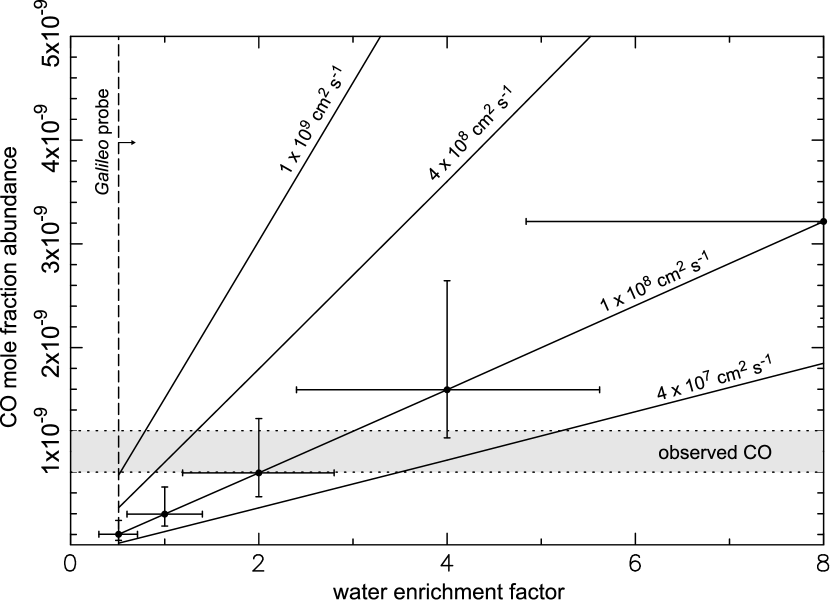
Figure 5: The quenched CO mole fraction derived from our model (solid lines) as a function of the water enrichment ($E_{\textrm{H}_{2}\textrm{O}}$) relative to the solar value of H₂O/H${}_{2}=9.61\times 10^{-4}$ for different values of $K_{zz}$ (as labeled). The dashed vertical line shows the water abundance measured by the Galileo entry probe (Wong et al., 2004). The shaded area indicates the observed CO mole fraction of $(1.0\pm 0.2)\times 10^{-9}$ reported by Bézard et al. (2002) and constrains the range of $K_{zz}$ and $E_{\textrm{H}_{2}\textrm{O}}$ values in Jupiter’s troposphere. The error bars for the $K_{zz}=1\times 10^{8}$ cm² s^-1 solution represent the estimated errors due to uncertainties in the reaction kinetics. Higher $K_{zz}$ values represent quenching and mixing from deeper in the atmosphere where CO is more abundant; higher water enrichments yield higher CO abundances at the quench level.

The quenched CO mole fraction also depends on the assumed deep water abundance. Figure 4 shows vertical abundance profiles for CO in Jupiter’s atmosphere for our assumed nominal $K_{zz}$ value of $1\times 10^{8}$ cm² s^-1 over a range of water enrichments, including the abundance measured by the Galileo entry probe (0.51x solar). The gray lines indicate the equilibrium abundance of carbon monoxide for different water enrichments; divergence from the equilibrium profiles occurs where fast atmospheric mixing and slow reaction kinetics (relative to one another) quench the CO mole fraction. For any single $K_{zz}$ profile, the pressure level at which quenching occurs is roughly independent of the H₂O abundance, over the range of water enrichments considered here. Therefore, for all the models shown in Fig. 4, the quench level occurs at similar pressure and temperature conditions. As discussed above, for otherwise constant conditions (e.g., P, T, K, [CH₄], [H₂]; see Eq. 16), the CO abundance is linearly proportional to the H₂O abundance in Jupiter’s deep atmosphere (see also Fig. 5). The quenched CO mole fraction thus increases as the assumed deep water abundance increases. For the assumption $K_{zz}=1\times 10^{8}$ cm² s^-1, Fig. 4 shows that the CO observations are best reproduced for a global water enrichment between 2-4 times solar.

Table 2 and Fig. 5 summarize the sensitivity of the quenched upper tropospheric CO mole fraction to variations in the two main free parameters of our kinetic/transport model: the atmospheric convective mixing rate (characterized by $K_{zz}$) and the tropospheric water inventory (characterized by $E_{\textrm{H}_{2}\textrm{O}}$). Taking the CO mole fraction as an observational constraint, we can constrain the deep H₂O abundance on Jupiter for a plausible range of eddy $K_{zz}$ values. For example, our model solutions are represented by the solid lines in Fig. 5. The slope of each line is proportional to $K_{zz}$ and hence the vertical convective mixing rate. The observed upper tropospheric CO mole fraction of $(1.0\pm 0.2)\times 10^{-9}$ (Bézard et al., 2002), represented by the shaded area, constrains the range of $K_{zz}$ and $E_{\textrm{H}_{2}\textrm{O}}$ values in our model solutions which are consistent with observations of CO in Jupiter’s troposphere.

For our nominal model with $K_{zz}$ = $1\times 10^{8}$ cm² s^-1, our results show that an H₂O abundance of 2.5 times the solar H₂O/H₂ ratio best reproduces the observed CO abundance. This enrichment corresponds to H₂O/H${}_{2}=2.4\times 10^{-3}$ or $X_{\textrm{H}_{2}\textrm{O}}=2.1\times 10^{-3}$ in Jupiter’s troposphere. If we further consider a range of plausible $K_{zz}$ values from $4\times 10^{7}$ to $1\times 10^{9}$ cm² s^-1 based on the theories described in Section 2.1, we find that H₂O/H₂ ratios between 0.52 and 5.20 times the solar ratio remain consistent with CO observations, including uncertainties in the observations themselves.

The above discussion does not consider the potential errors due to uncertainties in reaction kinetics and thermodynamic parameters. The error bars in Fig. 5 show our attempt to quantify the effect of these uncertainties. As described below (§3.2), the CO $\rightarrow$ CH₄ conversion is largely controlled by one rate-limiting step (reaction R863), for which the rate coefficient was derived using the rate coefficient of the reverse reaction (R862), as reported by Jodkowski et al. (1999) from ab initio calculations. However, no uncertainties were discussed for the calculated rate coefficient $k_{\textrm{\ref{R862}}}$. Based upon a literature search of theory-data comparisons for other reactions, we estimate that $k_{\textrm{\ref{R862}}}$ is uncertain by a factor of $\sim$3, which dominates over uncertainties in the thermodynamic parameters for the calculation of $k_{\textrm{\ref{R863}}}$. Including this estimated factor-of-three uncertainty in the reaction kinetics, our model results give a water enrichment of 0.3 to 7.3 times the solar abundance, corresponding to H₂O/H${}_{2}=(0.29-7.0)\times 10^{-3}$ and $X_{\textrm{H}_{2}\textrm{O}}=(0.25-6.0)\times 10^{-3}$. Thus, the subsolar water abundance (0.51x solar) measured by the Galileo entry probe (Wong et al., 2004) is plausibly consistent with the observed chemical behavior of carbon monoxide if relatively rapid vertical mixing rates (e.g., corresponding to $K_{zz}\sim 1\times 10^{9}$ cm² s^-1) prevail in Jupiter’s troposphere. For comparison, Bézard et al. (2002) derive a water abundance of H₂O/H${}_{2}=(0.34-15.3)\times 10^{-4}$ (0.4 to 15.9 times the solar abundance) using a timescale approach rather than a full kinetic-transport model. Refinement of our estimate for the water enrichment may require updated rate-constant measurements for key reactions in the CO reduction mechanism and improved constraints on the $K_{zz}$ profile in Jupiter’s troposphere.

3.2 Reaction Pathways for CO Destruction

In the present study we did not select the rate-determining step a priori, but rather we input a full reaction list and let the code identify the predominant (fastest) chemical pathway for net CO$\rightarrow$CH₄ conversion based upon the relative rates of all reactions included in the model. As discussed above (§2.4), reaction rate coefficients have been obtained from experimental or theoretical data available in the literature or calculated from the rate coefficient of the reverse reaction at each level in the model via Eq. (11). Empirical rate-constant expressions for the important reactions involving CO reduction in our kinetic scheme are listed in Table 3.

Our model results indicate that carbon monoxide reduction to methane in Jupiter’s atmosphere is dominated by the following series of reactions

$$\textrm{H}+\textrm{CO} \xrightarrow{\textrm{M}}\textrm{HCO}$$ (R742)

$$\textrm{H}_{2}+\textrm{HCO} \rightarrow\textrm{H}_{2}\textrm{CO}+\textrm{H}$$ (R787)

$$\textrm{H}+\textrm{H}_{2}\textrm{CO} \xrightarrow{\textrm{M}}\textrm{CH}_{3}\textrm{O}$$ (R831)

$$\textrm{H}_{2}+\textrm{CH}_{3}\textrm{O} \rightarrow\textrm{CH}_{3}\textrm{OH}+\textrm{H}$$ (R863)

$$\textrm{H}+\textrm{CH}_{3}\textrm{OH} \rightarrow\textrm{CH}_{3}+\textrm{H}_{2}\textrm{O}$$ (R858)

$$\textrm{H}_{2}+\textrm{CH}_{3} \rightarrow\textrm{CH}_{4}+\textrm{H}$$ (R151)

$$\textrm{CO}+3\,\textrm{H}_{2} \rightarrow\textrm{CH}_{4}+\textrm{H}_{2}\textrm{O}$$ (net)

where M refers to any third body (i.e., the reaction is termolecular) and the reaction numbers are the assigned reaction numbers in our kinetic model (see Table 3). This kinetic scheme differs considerably from that proposed by Prinn and Barshay (1977) and adopted by subsequent authors, which assumes that the rate-limiting step for converting CO to CH₄ is the reaction

$$\textrm{H}_{2}+\textrm{H}_{2}\textrm{CO}\rightarrow\textrm{CH}_{3}+\textrm{OH}.$$ (R669)

Prinn and Barshay (1977) calculated a rate constant for R669 using the rate of the reaction CH₃ + OH (Fenimore, 1969; Bowman, 1974), assuming that formaldehyde is a major product. However, a number of experimental and theoretical kinetic investigations over the past three decades demonstrate that the reaction channel forming H₂CO is insignificant in the reaction between methyl and hydroxyl radicals and that the rate estimated by Prinn and Barshay (1977) is incorrect (Bar-Nun and Podolak, 1985; Dean and Westmoreland, 1987; Yung et al., 1988; De Avillez Pereira et al., 1997; Xia et al., 2001; Krasnoperov and Michael, 2004; Baulch et al., 2005; Jasper et al., 2007), as has been noted in other studies of CO quenching kinetics (Yung et al., 1988; Griffith and Yelle, 1999; Bézard et al., 2002; Cooper and Showman, 2006). Updated second-order temperature-dependent rate coefficients for the reverse reaction OH + CH₃ $\rightarrow$ H₂CO + H₂ (R668) are now available from Dean and Westmoreland (1987) and De Avillez Pereira et al. (1997), and show that the rate coefficient for R669 is $\sim$3 orders of magnitude smaller than that estimated by Prinn and Barshay (1977) at quench-level temperatures ($\sim$1000 K) on Jupiter. Furthermore, we note that R669 is included in our model reaction list but that its contribution to CO destruction is insignificant, consistent with kinetics literature (e.g., Fenimore, 1969; Dean and Westmoreland, 1987; De Avillez Pereira et al., 1997; Xia et al., 2001; Krasnoperov and Michael, 2004; Baulch et al., 2005; Jasper et al., 2007), because faster, alternative reaction pathways exist for CO$\rightarrow$CH₄ conversion in Jupiter’s troposphere.

Our reaction scheme (in particular reactions R831 through R151) is similar to that proposed by Yung et al. (1988) and adopted by Griffith and Yelle (1999) for Gliese 229B and Bézard et al. (2002) for Jupiter. However, we find that H₂ + CH₃O $\rightarrow$ CH₃OH + H (reaction R863) is the slowest reaction in this dominant scheme and, as such, is the rate-limiting step, whereas Yung et al. (1988), Griffith and Yelle (1999), and Bézard et al. (2002) assumed H + H₂CO + M $\rightarrow$ CH₃O + M (R831) was the rate-limiting reaction for CO destruction. We also note that the activation energy for R863 at high temperatures ($\sim$90 kJ mol^-1 for 1600 to 3600 K) is similar to that measured by Bar-Nun and Shaviv (1975) and Bar-Nun and Podolak (1985) for CO reduction in high-temperature shocks. However, we are unable to confirm whether CO$\rightarrow$CH₄ conversion in the shock-tube experiments involves the same reaction pathways (R742 through R151) as we find for Jupiter (cf. Yung et al., 1988).

There are no experimental data available for R863, so we have determined its rate from the rate coefficient of the reverse reaction,

$$\textrm{H}+\textrm{CH}_{3}\textrm{OH}\rightarrow\textrm{CH}_{3}\textrm{O}+\textrm{H}_{2},$$ (R862)

as calculated by Jodkowski et al. (1999) using transition-state theory. Adopting $k_{\textrm{\ref{R862}}}$ as $k_{r}$ in equation (11) along with thermodynamic parameters for CH₃OH from Chen et al. (1977), H from Chase (1998), and CH₃O from Ruscic et al. (2005), we calculated the reaction rate coefficient for R863 at each temperature level in our model and determine an empirical fit of the form

$$k_{\textrm{\ref{R863}}}=1.77\times 10^{-22}T^{3.09}e^{(-3055/T)}.$$ (17)

We note that Jodkowski et al. (1999) also calculated $k_{\textrm{\ref{R863}}}$ from the rate coefficient of the reverse reaction, and estimate $k_{\textrm{\ref{R863}}}=2.10\times 10^{-25}T^{4.0}e^{-2470/T}$. However, Jodkowski et al. (1999) use equilibrium constants derived theoretically from molecular parameters, whereas we have taken advantage of the thermodynamic updates provided by Ruscic et al. (2005). Our value for $k_{\textrm{\ref{R863}}}$ therefore differs from that of Jodkowski et al. (1999), but by an amount that is much smaller than our overall factor-of-three estimated uncertainty in $k_{\textrm{\ref{R863}}}$ over the range of temperatures considered in our model. Our results regarding the quench point, and its constraint on the water enrichment, are particularly sensitive to the rate coefficient adopted for R863, and the factor-of-three uncertainty in $k_{\ref{R863}}$ has been included in the overall uncertainties in the deep water abundance we derive for Jupiter (see §3.1 and the error bars in Fig. 5). However, there are several alternative reactions, including R831, which may dominate if this rate is in serious error, in which case we would expect qualitatively similar results for CO quench chemistry in Jupiter’s troposphere (see note added in proof).

3.3 Validity of the Time-scale Approach

Having identified the dominant chemical mechanism for CO $\rightarrow$ CH₄ conversion in the Jovian troposphere, we can now test the validity of the time-scale approach previously used for estimating Jupiter’s deep water inventory (e.g., Prinn and Barshay, 1977; Fegley and Prinn, 1988; Bézard et al., 2002). The chemical lifetime for CO is given by the expression

$$t_{chem}\textrm{(CO)}=\frac{[\textrm{CO}]}{-d[\textrm{CO}]/dt}=\frac{\textrm{[CO]}}{k_{\textrm{\ref{R863}}}[\textrm{H}_{2}][\textrm{CH}_{3}\textrm{O}]},$$ (18)

assuming reaction R863 is the rate-limiting reaction. The vertical mixing time scale is given by

$$t_{mix}=\frac{L^{2}}{K_{zz}}$$ (19)

where $K_{zz}$ is the eddy diffusion coefficient and $L$ is the characteristic length scale over which the mixing operates. The atmospheric pressure scale height is traditionally used for $L$ for these types of calculations. However, Smith (1998) demonstrated theoretically that $L\approx H$ is not appropriate and may lead to over-estimates of the mixing length and the mixing time scale. Using the procedure recommended by Smith (1998), we obtain $L\sim 0.12H$ for CO quenching kinetics on Jupiter.

We have calculated the CO abundance at the quench level (i.e., where $t_{chem}=t_{mix}$) over a range of water enrichments (0.51x to 8x) and $K_{zz}$ values ($4\times 10^{7}$ to $1\times 10^{9}$ cm³ s^-1) for comparison with our kinetic model results. For $K_{zz}=1\times 10^{8}$ cm² s^-1 and $X_{\textrm{CO}}=(1.0\pm 0.2)\times 10^{-9}$ (Bézard et al., 2002), our time-scale approach yields a water enrichment of $2.9\pm 0.6$ times solar, whereas our nominal kinetic-transport model yields $E_{\textrm{H}_{2}\textrm{O}}=2.5\pm 0.5$ (not including uncertainties in $K_{zz}$ and $k_{\textrm{\ref{R863}}}$). Given the overall additional uncertainties in atmospheric mixing rates and reaction kinetics, we conclude that the back-of-the-envelope time-scale approach gives a reasonably accurate estimate of the H₂O abundance on Jupiter, provided that the vertical mixing length scale $L$ advocated by Smith (1998) is used and that the appropriate rate-limiting reaction and rate coefficient are considered. Regarding the latter point, we reemphasize that R863 is the rate-limiting reaction for CO destruction in our model, in contrast to the assumptions of previous investigators.

3.4 Chemistry of Other C–O Gases

Carbon monoxide is not the only species that will undergo quenching in Jupiter’s atmosphere. In principle, any atmospheric constituent subject to vertical transport and reaction chemistry will quench if the characteristic time scale for convective mixing becomes shorter than the characteristic time scale for kinetic destruction. Here we examine the chemical behavior of other oxidized carbon gases in Jupiter’s troposphere. Figure 6 shows the vertical abundance profiles for C–O species for a model in which $K_{zz}=1\times 10^{8}$ cm² s^-1 and $E_{\textrm{H}_{2}\textrm{O}}=1$. The dotted gray lines indicate abundances predicted by thermochemical equilibrium using the NASA CEA code; divergence from equilibrium is evident for CO, CO₂, H₂CO and CH₃O and illustrates where rapid vertical mixing and slow reaction kinetics (relative to one another) drives each species toward a constant quenched mole-fraction profile. Again, CH₄ and H₂O remain the dominant carbon- and oxygen-bearing gases, respectively, throughout Jupiter’s troposphere. The CO abundance begins to diverge from equilibrium near the 640-bar level and assumes a constant quenched profile at altitudes above the 200-bar level.

As pointed out by Prinn and Barshay (1977), reactions among oxidized (CO, CO₂, etc.) or reduced (CH₄,CH₃, etc.) carbon-bearing gases are expected to be much faster than reactions between these two families. As a result, the chemistry of many oxidized carbon gases is strongly tied to the chemical behavior of CO, the most abundant C–O compound in Jupiter’s atmosphere. For example, CO quenching (via the rate-limiting step R863) immediately affects the vertical abundance profile of CO₂. At altitudes above the level where CO begins to quench ($\sim$640 bar), CO₂ remains in equilibrium with CO via the reactions

$$\textrm{OH}+\textrm{CO} \rightarrow\textrm{CO}_{2}+\textrm{H}$$ (R708)

$$\textrm{H}+\textrm{CO}_{2} \rightarrow\textrm{CO}+\textrm{OH}\quad.$$ (R709)

The CO₂ abundance thus slightly increases with altitude until CO$\rightleftarrows$CO₂ conversion (via R708$\rightleftarrows$R709) itself quenches near the 500-bar level, whereupon CO₂ assumes a constant vertical profile to higher altitudes. Our upper-tropospheric result for CO₂ is similar to that of Lellouch et al. (2002), who used a time-scale approach to derive a quenched CO₂ mole fraction abundance of $3\times 10^{-12}$ for a solar O/H ratio in Jupiter’s troposphere.

Although methanol is one of the products of the rate-limiting reaction (R863) in our predominant kinetic scheme for CO$\rightarrow$CH₄ destruction, the vertical abundance profile for CH₃OH shows no dependence upon the chemical behavior of CO. This result can be explained by comparing the most important reactions for CH₃OH production at the 400-bar level (for example) in our nominal model:

$$\textrm{H}_{2}\textrm{O}+\textrm{CH}_{3} \rightarrow\textrm{CH}_{3}\textrm{OH}+\textrm{H} 93.5\%$$ (R859)

$$\textrm{H}_{2}+\textrm{CH}_{2}\textrm{OH} \rightarrow\textrm{CH}_{3}\textrm{OH}+\textrm{H} 6.3\%$$ (R861)

$$\textrm{H}_{2}+\textrm{CH}_{3}\textrm{O} \rightarrow\textrm{CH}_{3}\textrm{OH}+\textrm{H} 0.3\%$$ (R863)

Methanol production from CH₃ and H₂O via R859 far exceeds production via R863, so the chemical behavior of CH₃OH is largely decoupled from the CO$\rightarrow$CH₄ kinetic scheme (i.e., the carbon in CH₃OH comes predominantly from CH₄$\rightarrow$CH₃ rather than CO, and the oxygen comes from H₂O). The CH₃OH abundance follows an equilibrium profile until production via R859 quenches near the 200-bar level, at which point vertical mixing drives CH₃OH toward a constant mole-fraction profile.

The vertical abundance profile for H₂CO is more complex than that for the other C–O gases. At altitudes above the level where CO begins to quench, HCO remains in equilibrium with CO via R742$\rightleftarrows$R743 (see Table 3). In turn, the H₂CO abundance departs from its predicted equilibrium abundance profile and instead remains in approximate equilibrium with CO because formaldehyde production via the reactions (at the 400-bar level):

$$\textrm{H}_{2}+\textrm{HCO} \rightarrow\textrm{H}_{2}\textrm{CO}+\textrm{H} 82.5\%$$ (R787)

$$\textrm{CH}_{3}\textrm{O} \xrightarrow{\textrm{M}}\textrm{H}_{2}\textrm{CO}+\textrm{H} 17.5\%$$ (R830)

is balanced by destruction via the reactions:

$$\textrm{H}_{2}\textrm{CO}+\textrm{H} \rightarrow\textrm{HCO}+\textrm{H}_{2} 81.1\%$$ (R786)

$$\textrm{H}+\textrm{H}_{2}\textrm{CO} \xrightarrow{\textrm{M}}\textrm{CH}_{3}\textrm{O} 18.9\%$$ (R831)

This balance continues until conversion via R830$\rightleftarrows$R831 begins to quench near the 500 bar level and can no longer offset production and loss via HCO (R787$\rightleftarrows$R786), whereupon vertical atmospheric mixing drives H₂CO toward a constant quenched profile near the 100-bar level (a difference in altitude of roughly one pressure scale height). As a result (see Fig. 6), the H₂CO vertical abundance profile shows changes in response to two separate quenching reactions (R863 and R830) in Jupiter’s troposphere.

4 Discussion

4.1 Implications for Jupiter’s Total Oxygen Inventory

Water vapor is the dominant oxygen-bearing gas throughout Jupiter’s atmosphere and is much more abundant than other oxygen-bearing gases (CO, OH, etc.). For this reason, the H₂O abundance in the troposphere is expected to be representative of the majority of Jupiter’s total oxygen inventory. However, some oxygen ($\sim$20%) is removed from the gas phase by oxide formation (rock) in the deep atmosphere (e.g., Fegley and Prinn, 1988; Lodders, 2004; Visscher and Fegley, 2005). This removal must be considered before evaluating the bulk planetary oxygen abundance and, in turn, the heavy-element composition of planetesimals during Jupiter’s formation.

The fraction of oxygen removed by rock depends upon the abundance of all rock-forming elements (Mg, Si, Ca, Al, Na, K, Ti) relative to the total oxygen abundance. Following the method of Visscher and Fegley (2005), and using updated solar abundances from Lodders et al. (2009), the relative abundances of water vapor, total oxygen, and the rock-forming elements can be written as

$$E_{\textrm{H}_{2}\textrm{O}}=1.261E_{\Sigma{\textrm{O}}}-0.261E_{\textrm{rock}}$$ (20)

where $E_{i}$ represents the enrichment (over solar ratios) for each component $i$. This expression serves as a general mass-balance constraint for the relative abundances of water, oxygen, and rock over a range of heavy element enrichments in Jupiter’s interior (Visscher and Fegley, 2005). To derive this expression, it was assumed that all of the rock-forming elements are equally enriched, and $E_{\textrm{rock}}=2.74\pm 0.65$ was adopted based upon the “deep” tropospheric abundance of sulfur (as H₂S; Wong et al., 2004), which behaves as a rock-forming element in meteorites (Lodders, 2004). Using $E_{\textrm{rock}}=2.74\pm 0.65$ in equation (20) along with the Galileo entry probe H₂O abundance of $E_{\textrm{H}_{2}\textrm{O}}=0.51\pm 0.17$ (see Table 1) yields a total oxygen abundance (characterized by $E_{\Sigma\textrm{O}}$) of $0.97\pm 0.40$ times the solar abundance of $\Sigma\textrm{O}/\textrm{H}_{2}=1.212\times 10^{-3}$.

Using our nominal model result of $E_{\textrm{H}_{2}\textrm{O}}=2.5\pm 0.5$, equation (20) yields a total oxygen enrichment of $E_{\Sigma\textrm{O}}=2.5\pm 0.8$. Further considering a 3x uncertainty in reaction kinetics and a range of plausible $K_{zz}$ values from $4\times 10^{7}$ to $1\times 10^{9}$ cm² s^-1, our water constraint (0.3 – 7.3x solar) gives a total oxygen inventory of 0.7 to 6.5 times the solar $\Sigma\textrm{O}/\textrm{H}_{2}$ ratio in Jupiter’s interior. This value represents the bulk oxygen inventory of Jupiter’s interior consistent with CO chemistry, and includes oxygen as water plus oxygen bound in rock.

4.2 Implications for Planetary Formation

All viable giant-planet formation models must consider how heavy elements become entrained in the planet during its formation and evolution. An important constraint for such models is therefore the observed atmospheric abundances of gases such as CH₄, NH₃, H₂S, PH₃, and H₂O, which are taken to represent the planetary elemental inventories of C, N, S, P, and the majority of planetary oxygen, respectively. As illustrated in Fig. 7, observations of Jupiter’s atmosphere show that C, N, S, P, Ar, Kr, and Xe are enhanced relative to solar element-to-hydrogen ratios (Mahaffy et al., 2000; Wong et al., 2004; Lodders, 2004) by factors of 2-4. The enrichment in heavy elements is generally believed to be consistent with the core-accretion model for giant planet formation (Mizuno, 1980), in which a rock or rock-ice core initially forms and continues to grow through the accretion of solid planetesimals until it is massive enough to capture nebular gas (Bodenheimer and Pollack, 1986; Lissauer, 1987; Pollack et al., 1996). In this scenario, the observed heavy element enrichments on Jupiter arise from degassing of the initial core material and the continued accretion of solid planetesimals, which will most likely vaporize before reaching the core (e.g., Pollack et al., 1986). What remains unclear is the source and composition of the planetesimals which provided the enrichment, and several scenarios have been proposed to explain the observed heavy-element abundances.

One distinguishing characteristic of Jovian formation scenarios is the predicted water inventory in Jupiter’s deep atmosphere. For example, trapping of heavy elements by hypothetical solar-composition icy planetesimals (Owen et al., 1999; Atreya et al., 2003; Owen and Encrenaz, 2006) would be expected to give an enrichment in oxygen (as H₂O) around 3$\pm$1 times solar, similar that for the other heavy elements. Trapping of heavy elements in the form of clathrate hydrates near the snow line (e.g. Lunine and Stevenson, 1985; Gautier et al., 2001a; Hersant et al., 2004) would yield higher water abundances, with predicted enrichments ranging from $\sim$6 (Mousis et al., 2009) to $\sim$8 (Alibert et al., 2005) to as high as $\gtrsim$17 (Gautier et al., 2001a, b) or $\sim$19 (Hersant et al., 2004) times the solar H₂O/H₂ ratio of $9.61\times 10^{-4}$. Accretion of carbon-rich planetesimals behind a nebular “tar line” (Lodders, 2004) would give subsolar water abundances similar to that observed by the Galileo probe (0.51x solar).

Our indirect constraint of a deep water abundance 0.3–7.3 times the solar H₂O/H₂ ratio from our kinetic-transport model is plausibly consistent with each of these formation mechanisms but precludes clathrate-hydrate scenarios that would require large ($>\,$8x) water enrichments in Jupiter’s deep atmosphere (e.g., Gautier et al., 2001a, b; Hersant et al., 2004; Alibert et al., 2005).

5 Summary

We have developed a comprehensive thermochemical kinetics and diffusion model for Jupiter which correctly transitions between equilibrium chemistry in the deep troposphere and quenched/disequilibrium chemistry in the upper troposphere. We use this numerical model to compute the vertical abundance profiles for all carbon- and oxygen-bearing atmospheric constituents and to explore the chemical behavior of CO and other oxidized carbon species in Jupiter’s deep atmosphere. We find that carbon monoxide is reduced to CH₄ via a mechanism similar to that proposed by Yung et al. (1988); however, our model indicates that the rate-limiting reaction for CO reduction in Jupiter’s atmosphere is H₂ + CH₃O $\rightarrow$ CH₃OH + H rather than Yung et al.’s proposed reaction H + CH₃O + M $\rightarrow$ CH₃OH + M. We also confirm the original analytic prediction of Prinn and Barshay (1977) that the mole fraction of CO will “quench” and remain constant with altitude when kinetic reaction rates can no longer compete with atmospheric mixing. This quenching occurs at the $\sim$400 bar (1000 K) level in our nominal model. Carbon monoxide is not the only species to quench; virtually all atmospheric constituents will quench at some point where temperatures become low enough to inhibit the kinetics.

Our kinetic-transport model quantitatively confirms the convenient, back-of-the-envelope time-scale approach currently used to explore quenched disequilibrium chemistry on giant planets and brown dwarfs (e.g., Prinn and Barshay, 1977; Lewis and Fegley, 1984; Fegley and Prinn, 1985, 1988; Lodders and Fegley, 1994, 2002; Griffith and Yelle, 1999; Bézard et al., 2002; Visscher and Fegley, 2005). We find that the the time-scale approach is valid for estimating Jupiter’s water inventory, provided that the correct rate-limiting reaction is considered (which we find to be reaction R863, H₂ + CH₃O $\rightarrow$ CH₃OH + H) and provided that the mixing length $L$ is determined via the procedure advocated by Smith (1998).

Using the CO abundance reported by Bézard et al. (2002) as our observational constraint, our model-data comparisons indirectly constrain the Jovian deep water abundance to lie in the range 0.3–7.3 times the solar H₂O/H₂ ratio of $9.61\times 10^{-4}$. Our results suggest that the enrichment for oxygen (as H₂O) is similar, to within uncertainties, as that for carbon, nitrogen, and other heavy elements — giant-planet formation scenarios that require very large ($>\,$8x) enrichments in the water abundance (such as some clathrate-hydrate formation scenarios) are precluded. The subsolar water abundance (0.51x solar) measured by the Galileo entry probe (Wong et al., 2004) remains plausibly consistent with the observed tropospheric abundance of carbon monoxide if relatively rapid vertical mixing (e.g., $K_{zz}\ \gtrsim 1\times 10^{9}$ cm² s^-1) prevails in Jupiter’s deep troposphere.

We will not be able to narrow our estimated range of Jovian deep water enrichments without experimental confirmation of the rate coefficient for the reaction of methoxy with H₂ (CH₃O + H₂ $\rightarrow$ CH₃OH + H) at high pressures, for temperatures near 1000 K, and our results are subject to revision as updated kinetics data become available. Perhaps more importantly, we need a better understanding of appropriate diffusion coefficients that can be used to represent convective processes under tropospheric conditions on Jupiter. The Juno mission may provide microwave data (Janssen et al., 2005; Bolton et al., 2006) that can be used to test our model prediction regarding the Jovian deep water abundance.

We point out that oxygen species are not the only constituents to quench in our model; the quenching of nitrogen species like N₂ and HCN is interesting in its own right and will be the subject of a future investigation. Our kinetics-transport model can easily be applied to other giant planets and brown dwarfs. Of particular interest is (1) constraining the deep water abundance on the other giant planets in our own solar system from current or future tropospheric CO observations (which must be able to constrain the vertical profile to separate the contributions arising from possible internal and external sources), as no current plans to send multiprobe missions to these planets are on schedule for the near future, and (2) predicting the vertical variation of observable species in brown dwarfs and extrasolar giant planets, as these atmospheres are unlikely to be in complete thermochemical equilibrium.

Table 1: Gas Abundances in Jupiter’s Troposphere

Gas $i$	Jupiter $i$/H2	Reference	Protosolar $i$/H2${}^{\textrm{a}}$	Enrichment Factor
H2	$\equiv 1$		$\equiv 1$	$\equiv 1$
He	$0.1574\pm 0.0036$	b, c	0.1938	$0.81\pm 0.02$
CH4	$(2.37\pm 0.57)\times 10^{-3}$	d	$5.55\times 10^{-4}$	$4.27\pm 1.03$
NH3	$(6.64\pm 2.54)\times 10^{-4}$	d	$1.64\times 10^{-4}$	$4.05\pm 1.55$
H2O	$(4.9\pm 1.6)\times 10^{-4}$	d	$9.61\times 10^{-4}$	$0.51\pm 0.17$
PH3	$(0.8\pm 0.5)\times 10^{-6}$	e	$6.41\times 10^{-7}$	$1.25\pm 0.78$
H2S	$(8.9\pm 2.1)\times 10^{-5}$	d	$3.25\times 10^{-5}$	$2.74\pm 0.65$
Ar	$(1.82\pm 0.36)\times 10^{-5}$	f	$7.16\times 10^{-6}$	$2.54\pm 0.50$
Kr	$(9.30\pm 1.70)\times 10^{-9}$	f	$4.31\times 10^{-9}$	$2.16\pm 0.39$
Xe	$(8.90\pm 1.70)\times 10^{-10}$	f	$4.21\times 10^{-10}$	$2.11\pm 0.40$

Note. References: (a) Protosolar abundances from Lodders et al. (2009) (b) Niemann et al. (1998), (c) von Zahn et al. (1998), (d) Wong et al. (2004), (e) 5-$\mu$m spectroscopy, see text (f) Mahaffy et al. (2000).

Table 2: Quenched CO Mole Fraction ($X_{\textrm{CO}}$) for Variations in $K_{zz}$ and $E_{\textrm{H}_{2}\textrm{O}}$

H2O	Eddy Diffusion Coefficient $K_{zz}$ (cm2 s-1)
enrichmenta	$4\times 10^{7}$	$1\times 10^{8}$	$4\times 10^{8}$	$1\times 10^{9}$
0.51x	$1.16\times 10^{-10}$	$2.02\times 10^{-10}$	$4.57\times 10^{-10}$	$7.71\times 10^{-10}$
1x	$2.28\times 10^{-10}$	$3.96\times 10^{-10}$	$8.95\times 10^{-10}$	$1.51\times 10^{-9}$
2x	$4.57\times 10^{-10}$	$7.93\times 10^{-10}$	$1.79\times 10^{-9}$	$3.03\times 10^{-9}$
4x	$9.18\times 10^{-10}$	$1.59\times 10^{-9}$	$3.60\times 10^{-9}$	$6.08\times 10^{-9}$
8x	$1.85\times 10^{-9}$	$3.22\times 10^{-9}$	$7.27\times 10^{-9}$	$1.23\times 10^{-8}$

^aWater enrichment factor ($E_{\textrm{H}_{2}\textrm{O}}$) relative to a solar H₂O/H₂ ratio of $9.61\times 10^{-4}$. The Galileo entry probe measured a deep Jovian water abundance of 0.51x solar (Wong et al., 2004). The observed mole fraction of CO in Jupiter’s atmosphere is $X_{\textrm{CO}}=(1.0\pm 0.2)\times 10^{-9}$ (Bézard et al., 2002).

Table 3: Important Reaction Pathways for CO$\rightleftarrows$CH₄ in Jupiter’s Atmosphere

	Reaction			Rate Constant	Reference
R742	$\textrm{H}+\textrm{CO}$	$\xrightarrow{\textrm{M}}$	HCO	$k_{0}=5.30\times 10^{-34}e^{(-370/T)}$	Baulch et al. (1994)
				$k_{\infty}=1.96\times 10^{-13}e^{(-1366/T})$	Arai et al. (1981)
R743	HCO	$\xrightarrow{\textrm{M}}$	$\textrm{CO}+\textrm{H}$	$k_{0}=4.18\times 10^{-9}T^{-0.36}e^{(-8294/T)}$	reverse of R742
				$k_{\infty}=1.54\times 10^{12}T^{-0.36}e^{(-9290/T})$	reverse of R742
R786	$\textrm{H}+\textrm{H}_{2}\textrm{CO}$	$\rightarrow$	$\textrm{HCO}+\textrm{H}_{2}$	$k_{\textrm{R786}}=9.53\times 10^{-17}T^{1.90}e^{(-1379/T)}$	Irdam et al. (1993)
R787	$\textrm{H}_{2}+\textrm{HCO}$	$\rightarrow$	$\textrm{H}_{2}\textrm{CO}+\textrm{H}$	$k_{\textrm{R787}}=3.92\times 10^{-19}T^{2.23}e^{(-9082/T)}$	reverse of R786
R830	$\textrm{CH}_{3}\textrm{O}$	$\xrightarrow{\textrm{M}}$	$\textrm{H}_{2}\textrm{CO}+\textrm{H}$	$k_{0}=1.40\times 10^{-6}T^{-1.20}e^{(-7800/T)}$	Page et al. (1989)
				$k_{\infty}=1.50\times 10^{11}Te^{(-12880/T)}$	Bézard et al. (2002)
R831	$\textrm{H}+\textrm{H}_{2}\textrm{CO}$	$\xrightarrow{\textrm{M}}$	$\textrm{CH}_{3}\textrm{O}$	$k_{0}=1.28\times 10^{-33}T^{-0.30}e^{(3074/T)}$	reverse of R830
				$k_{\infty}=1.37\times 10^{-16}T^{1.90}e^{(-2006/T)}$	reverse of R830
R862	$\textrm{H}+\textrm{CH}_{3}\textrm{OH}$	$\rightarrow$	$\textrm{CH}_{3}\textrm{O}+\textrm{H}_{2}$	$k_{\textrm{R862}}=1.135\times 10^{-22}T^{3.40}e^{(-3640/T)}$	Jodkowski et al. (1999)
R863	$\textrm{H}_{2}+\textrm{CH}_{3}\textrm{O}$	$\rightarrow$	$\textrm{CH}_{3}\textrm{OH}+\textrm{H}$	$k_{\textrm{R863}}=1.77\times 10^{-22}T^{3.09}e^{(-3055/T)}$	reverse of R862
R858a	$\textrm{H}+\textrm{CH}_{3}\textrm{OH}$	$\rightarrow$	$\textrm{CH}_{3}+\textrm{H}_{2}\textrm{O}$	$k_{\textrm{R858}}=3.321\times 10^{-10}e^{(-2670/T)}$	Hidaka et al. (1989)
R859	$\textrm{H}_{2}\textrm{O}+\textrm{CH}_{3}$	$\rightarrow$	$\textrm{CH}_{3}\textrm{OH}+\textrm{H}$	$k_{\textrm{R859}}=5.83\times 10^{-15}Te^{(-15474/T)}$	reverse of R858
R150	$\textrm{H}+\textrm{CH}_{4}$	$\rightarrow$	$\textrm{CH}_{3}+\textrm{H}_{2}$	$k_{\textrm{R150}}=2.20\times 10^{-20}T^{3.00}e^{(-4045/T)}$	Baulch et al. (1992)
R151	$\textrm{H}_{2}+\textrm{CH}_{3}$	$\rightarrow$	$\textrm{CH}_{4}+\textrm{H}$	$k_{\textrm{R151}}=8.62\times 10^{-24}T^{3.57}e^{(-2995/T)}$	reverse of R150

Note – Reaction numbers in bold refer to steps in the dominant CO$\rightarrow$CH₄ kinetic scheme. Rate constants for bimolecular reactions ($k_{i}$ for reaction $i$) and high-pressure limiting rate constants for termolecular reactions ($k_{\infty}$) are in units of cm³ s^-1. Low-pressure limiting rate constants for termolecular reactions ($k_{0}$) are in units of cm⁶ s^-1. For decomposition reactions (e.g., R743 and R830), $k_{0}$ is in units of cm³ s^-1 and $k_{\infty}$ is in units of s^-1. Note that although the rate coefficients were internally reversed within our code, we provide empirical fits to the reaction rate coefficient expressions (valid for $T=$ 400 to 2500 K) for reverse reactions as an aid to other investigators. ^aSee note added in proof.

Table 4: Model results for variations in $\textrm{H}+\textrm{CH}_{3}\textrm{OH}$ reaction kinetics

$E_{\textrm{H}_{2}\textrm{O}}$	RLS	Rate Coefficients for H + CH3OH Reaction Pathwaysa
		$k_{\textrm{860}}$	$k_{\textrm{862}}$	$k_{\textrm{858}}$
0.4–3.4	R863	$2.249\times 10^{-21}T^{3.2}e^{(-1755/T)}$	$1.135\times 10^{-22}T^{3.4}e^{(-3640/T)}$	$9.41\times 10^{-9}e^{(-12400/T)}$
		Jodkowski et al. (1999)	Jodkowski et al. (1999)	$k_{\textrm{R860}}/k_{\textrm{R858}}=40$ at 1000 K
0.5–4.8	R863	$5.47\times 10^{-15}T^{1.24}e^{(-2260/T)}$	$2.28\times 10^{-16}T^{1.24}e^{(-2260/T)}$	$1.82\times 10^{-8}e^{(-12400/T)}$
		Baulch et al. (2005), assuming $k_{\textrm{R860}}/k_{\textrm{R862}}=24^{b}$		$k_{\textrm{R860}}/k_{\textrm{R858}}=40$ at 1000 K
0.6–5.3	R858	$2.72\times 10^{-17}T^{2}e^{(-2273/T)}$	$6.33\times 10^{-17}T^{2}e^{(-2947/T)}$	$1.70\times 10^{-8}e^{(-12400/T)}$
		Li and Williams (1996), $k_{\textrm{R860}}/k_{\textrm{R862}}=0.43e^{674/T}$		$k_{\textrm{R860}}/k_{\textrm{R858}}=40$ at 1000 K
0.1–1.2	R858	$4.23\times 10^{-10}e^{(-3516/T)}$	$1.19\times 10^{-10}e^{(-5549/T)}$	$5.08\times 10^{-10}e^{(-12400/T)}$
		Lendvay et al. (1997)	Lendvay et al. (1997)	Lendvay et al. (1997)
0.6–5.0	R858	$4.56\times 10^{-15}T^{1.24}e^{(-2260/T)}$	$1.14\times 10^{-15}T^{1.24}e^{(-2260/T)}$	$1.52\times 10^{-8}e^{(-12400/T)}$
		Baulch et al. (2005), assuming $k_{\textrm{R860}}/k_{\textrm{R862}}=4^{c}$		$k_{\textrm{R860}}/k_{\textrm{R858}}=40$ at 1000 K
0.7–6.2	R831	$2.82\times 10^{-17}T^{2.1}e^{(-2450/T)}$	$7.04\times 10^{-18}T^{2.1}e^{(-2450/T)}$	$2.94\times 10^{-8}e^{(-12400/T)}$
		Tsang (1987), $k_{\textrm{R860}}/k_{\textrm{R862}}=4$		$k_{\textrm{R860}}/k_{\textrm{R858}}=40$ at 1000 K

Note – ^aRate coefficients are in units of cm³ s^-1 for bimolecular reactions. ^bBased upon Carvalho et al. (2008). ^cBased upon Tsang (1987).

Figure 2: Carbon equilibrium chemistry for CH₄/H₂ = $2.37\times 10^{{-3}}$ (Wong et al., 2004) and H₂O/H₂ = $2.40\times 10^{{-3}}$ (2.5x solar) in Jupiter’s atmosphere, calculated using the NASA CEA code. Modeled after Fig. 17 in Fegley and Lodders (1994) for a slightly different atmospheric composition and revised thermodynamic parameters for H₂CO and CH₂.

Figure 4: Vertical profiles for CO and CH₄ in Jupiter’s atmospere for an assumed eddy diffusion coefficient $K_{zz}=1\times 10^{8}$ cm² s^-1 (our nominal model) and for various assumed water enrichments ($E_{\textrm{H}_{2}\textrm{O}}$) of 0.51 (GPMS value; dotted line), 1 (dot-dot-dot-dash line), 2 (dash-dot line) and 4 times (solid line) the solar H₂O/H₂ ratio of $9.61\times 10^{-4}$ (Lodders, 2004; Lodders et al., 2009). The corresponding gray lines show the CO abundance predicted by chemical equilibrium using the NASA CEA code. The circle with error bars represents the observed upper tropospheric CO mole fraction reported by Bézard et al. (2002). Note that for our assumed nominal value of $K_{zz}=1\times 10^{8}$ cm² s^-1, the CO observations are best reproduced for assumed global water enrichments of 2-4 times solar.

Figure 6: Vertical abundance profiles for oxidized carbon gases in Jupiter’s atmosphere for $K_{zz}=1\times 10^{8}$ cm² s^-1 and H₂O/H${}_{2}=9.61\times 10^{-4}$ (1x solar). The dotted gray lines indicate thermochemical equilibrium; divergence from the equilibrium profiles (shown here for CO, CO₂, H₂CO and CH₃OH) show where rapid vertical mixing and slow reaction kinetics drive each species to a constant quenched profile. For HCO, CH₂OH, and CH₃O, disequilibrium mixing occurs at much lower abundances (not shown).

Figure 7: Observed Jovian heavy element enrichments relative to solar (filled circles), as measured by the Galileo entry probe (C as CH₄, N as NH₃, O as H₂O, S as H₂S, Ar, Kr, Xe; Wong et al., 2004; Mahaffy et al., 2000) and infrared spectroscopy (P as PH₃, see §2.3), along with our kinetics-transport model results (open circle) for O as H₂O. Solar heavy element-to-hydrogen abundance ratios are taken from Lodders et al. (2009). The water enrichments are defined relative to a solar water abundance of H₂O/H${}_{2}=9.61\times 10^{-4}$ (see text for details).

References

- Alibert et al. (2005) Alibert, Y., Mousis, O., Benz, W., 2005. On the volatile enrichments and composition of Jupiter. Astrophys. J. Lett. 622, L145–L148.
- Allen et al. (1981) Allen, M., Yung, Y. L., Waters, J. W., 1981. Vertical transport and photochemistry in the terrestrial mesosphere and lower thermosphere (50-120 km). J. Geophys. Res. 86, 3617–3627.
- Arai et al. (1981) Arai, H., Nagai, S., Hatada, M., 1981. Radiolysis of methane containing small amounts of carbon monoxide-formation of organic acids. Radiat. Phys. Chem. 17, 211–216.
- Aronowitz et al. (1977) Aronowitz, D., Naegeli, D. W., Glassman, I., 1977. Kinetics of the pyrolysis of methanol. J. Phys. Chem. 81 (25), 2555–2559.
- Atreya (2004) Atreya, S. K., 2004. Composition, clouds, and origin of Jupiter’s atmosphere - a case for deep multiprobes into giant planets. In: A. Wilson (Ed.), Planetary Probe Atmospheric Entry and Descent Trajectory Analysis and Science. Vol. 544 of ESA Special Publication. pp. 57–62.
- Atreya et al. (2003) Atreya, S. K., Mahaffy, P. R., Niemann, H. B., Wong, M. H., Owen, T. C., 2003. Composition and origin of the atmosphere of Jupiter - An update, and implications for the extrasolar giant planets. Planet. Space Sci. 51, 105–112.
- Bar-Nun and Podolak (1985) Bar-Nun, A., Podolak, M., 1985. The contribution by thunderstorms to the abundances of CO, C2H2, and HCN on Jupiter. Icarus 64, 112–124.
- Bar-Nun and Shaviv (1975) Bar-Nun, A., Shaviv, A., 1975. Dynamics of the chemical evolution of Earth’s primitive atmosphere. Icarus 24, 197–210.
- Barshay and Lewis (1978) Barshay, S. S., Lewis, J. S., 1978. Chemical structure of the deep atmosphere of Jupiter. Icarus 33, 593–611.
- Baulch et al. (2005) Baulch, D. L., Bowman, C. T., Cobos, C. J., Cox, R. A., Just, T., Kerr, J. A., Pilling, M. J., Stocker, D., Troe, J., Tsang, W., Walker, R. W., Warnatz, J., 2005. Evaluated kinetic data for combustion modeling: Supplement ii. J. Phys. Chem. Ref. Data 34, 757–1397.
- Baulch et al. (1994) Baulch, D. L., Cobos, C. J., Cox, R. A., Frank, P., Hayman, G., Just, T., Kerr, J. A., Murrells, T., Pilling, M. J., Troe, J., Walker, R. W., Warnatz, J., 1994. Evaluated kinetic data for combustion modeling. supplement i. J. Phys. Chem. Ref. Data 23, 847–848.
- Baulch et al. (1992) Baulch, D. L., Cobos, C. J. Cox, R. A., Esser, C., Frank, P., Just, T., Kerr, J. A., Pilling, M. J., Troe, J., Walker, R. W., Warnatz, J., 1992. Evaluated kinetic data for combustion modelling. J. Phys. Chem. Ref. Data 21, 411–429.
- Beer (1975) Beer, R., Sep. 1975. Detection of carbon monoxide in Jupiter. Astrophys. J. Lett. 200, L167–L169.
- Beer and Taylor (1978) Beer, R., Taylor, F. W., 1978. The abundance of carbon monoxide in Jupiter. Astrophys. J. 221, 1100–1109.
- Bézard et al. (2002) Bézard, B., Lellouch, E., Strobel, D., Maillard, J.-P., Drossart, P., 2002. Carbon monoxide on Jupiter: Evidence for both internal and external sources. Icarus 159, 95–111.
- Bjoraker et al. (1986) Bjoraker, G. L., Larson, H. P., Kunde, V. G., 1986. The gas composition of Jupiter derived from 5 micron airborne spectroscopic observations. Icarus 66, 579–609.
- Bodenheimer and Pollack (1986) Bodenheimer, P., Pollack, J. B., 1986. Calculations of the accretion and evolution of giant planets The effects of solid cores. Icarus 67, 391–408.
- Bolton et al. (2006) Bolton, S., and the Juno Science Team, 2006. The Juno New Frontiers Jupiter polar orbiter mission. European Planetary Science Congress 2006, 535.
- Bowman (1974) Bowman, C. T. 1974. Non-equilibrium radical concentrations in shock-initiated methane oxidation. 15th International Symposium on Combustion (Combustion Institute, Pittsburgh), 869–882.
- Burcat and Ruscic (2005) Burcat, A., Ruscic, B., 2005. Third millenium ideal gas and condensed phase thermochemical database for combustion with updates from active thermochemical tables. TAE 960, ANL-05/20, Argonne National Laboratory. 26 pp.
- Carvalho et al. (2008) Carvalho, E. F. V., Barauna, A. N., Machado, F. B. C., Roberto-Neto, O., 2008. Theoretical calculations of energetics, structures, and rate constants for the H + CH3OH hydrogen abstraction reactions. Chem. Phys. Lett. 463, 33–37.
- Chase (1998) Chase, M. W., 1998. NIST-JANAF thermochemical tables. J. Phys. Chem. Ref. Data, 28, monograph no. 9. 1951 pp.
- Chen et al. (1977) Chen, S., Wilhoit, R., Zwolinski, B., 1977. Thermodynamic properties of normal and deuterated methanols. J. Phys. Chem. Ref. Data 6 (1), 105–112.
- Cooper and Showman (2006) Cooper, C. S., Showman, A. P., 2006. Dynamics and Disequilibrium Carbon Chemistry in Hot Jupiter Atmospheres, with Application to HD 209458b. Astrophys. J. Lett. 649, 1048–1063.
- da Silva et al. (2006) da Silva, G., Bozzelli, J., Sebbar , N., Bockhorn, H., 2006. Thermodynamic and Ab Initio Analysis of the Controversial Enthalpy of Formation of Formaldehyde. ChemPhysChem 7, 1119–1126.
- De Avillez Pereira et al. (1997) De Avillez Pereira, R., Baulch, D., Pilling, M., Robertson, S., Zeng, G., 1997. Temperature and Pressure Dependence of the Multichannel Rate Coefficients for the CH3 + OH System. J. Phys. Chem. A 101, 9681–9693.
- de Pater et al. (2005) de Pater, I., Deboer, D., Marley, M., Freedman, R., Young, R., 2005. Retrieval of water in Jupiter’s deep atmosphere using microwave spectra of its brightness temperature. Icarus 173, 425–438.
- Dean and Westmoreland (1987) Dean, A., Westmoreland, P., 1987. Bimolecular QRRK analysis of methyl radical reactions. Int. J. Chem. Kinet. 19, 207–228.
- Dean and Bozzelli (2000) Dean, A. M., Bozzelli, J. W., 2000. Combustion Chemistry of Nitrogen. In: Gardiner, W. C., J. (Ed.), Gas-Phase Combustion Chemistry. Springer: New York, pp. 125–342.
- DeMore et al. (1992) DeMore, W. B., Sander, S. P., Golden, D. M., Hampson, R. F., Kurylo, M. J., Howard, C. J., Ravishankara, A. R., Kolb, C. J., Molina, M. J., 1992. Chemical Kinetic and Photochemical Data for Use in Stratospheric Modelling: Evaluation No. 10. JPL Publication 92-20, Jet Propulsion Laboratory, Pasadena, CA. 269 pp.
- Drossart and Encrenaz (1982) Drossart, P., Encrenaz, T., 1982. The abundance of water on Jupiter from the Voyager IRIS data at 5 microns. Icarus 52, 483–491.
- Encrenaz et al. (1996) Encrenaz, T., de Graauw, T., Schaeidt, S., Lellouch, E., Feuchtgruber, H., Beintema, D. A., Bézard, B., Drossart, P., Griffin, M., Heras, A., Kessler, M., Leech, K., Morris, P., Roelfsema, P. R., Roos-Serote, M., Salama, A., Vandenbussche, B., Valentijn, E. A., Davis, G. R., Naylor, D. A., 1996. First results of ISO-SWS observations of Jupiter. Astron. Astrophys. 315, L397–L400.
- Fegley and Prinn (1983) Fegley, B., Jr., Prinn, R. G., 1983. Chemical Probes of Saturn’s Deep Atmosphere. LPSC Abstracts 14, 189–190.
- Fegley and Lodders (1994) Fegley, B., Jr., Lodders, K., 1994. Chemical models of the deep atmospheres of Jupiter and Saturn. Icarus 110, 117–154.
- Fegley and Prinn (1985) Fegley, B., Jr., Prinn, R. G., 1985. Equilibrium and nonequilibrium chemistry of Saturn’s atmosphere - Implications for the observability of PH3, N2, CO, and GeH4. Astrophys. J. 299, 1067–1078.
- Fegley and Prinn (1988) Fegley, B., Jr., Prinn, R. G., 1988. Chemical constraints on the water and total oxygen abundances in the deep atmosphere of Jupiter. Astrophys. J. 324, 621–625.
- Fenimore (1969) Fenimore, C., 1969. Destruction of methane in water gas by reaction of CH3 with OH radicals. 12th International Symposium on Combustion (Combustion Institute, Pittsburgh), 463–467.
- Fernando et al. (1991) Fernando, H. J. S., Chen, R. R., Boyer, D. L., 1991. Effects of rotation on convective turbulence. J. Fluid Mech. 228, 513–547.
- Flasar and Gierasch (1977) Flasar, F. M., Gierasch, P. J., 1977. Eddy diffusivities within Jupiter. In: Jones, A. V. (Ed.), Planetary Atmospheres. Proceedings of the Nineteenth Symposium of the Royal Society of Canada. Ottawa: Royal Society of Canada, p. 85.
- Flasar and Gierasch (1978) Flasar, F. M., Gierasch, P. J., 1978. Turbulent convection within rapidly rotating superadiabatic fluids with horizontal temperature gradients. Geophys. Astro. Fluid 10, 175–212.
- Gardiner (2000) Gardiner, W. C., J. (Ed.), 2000. Gas-Phase Combustion Chemistry. Springer-Verlag: New York. 543 pp.
- Gautier et al. (2001a) Gautier, D., Hersant, F., Mousis, O., Lunine, J. I., 2001a. Enrichments in volatiles in Jupiter: A new interpretation of the Galileo measurements. Astrophys. J. Lett. 550, L227–L230.
- Gautier et al. (2001b) Gautier, D., Hersant, F., Mousis, O., Lunine, J. I., Oct. 2001b. Erratum: Enrichments in Volatiles in Jupiter: A New Interpretation of the Galileo Measurements. Astrophys. J. Lett. 559, L183–L183.
- Gierasch and Conrath (1985) Gierasch, P. J., Conrath, B. J., 1985. Energy conversion processes in the outer planets. In: Hunt, G. E. (Ed.), Recent Advances in Planetary Meteorology. Cambrdige: Cambridge Univ. Press, pp. 121–146.
- Gladstone et al. (1996) Gladstone, G. R., Allen, M., Yung, Y. L., 1996. Hydrocarbon photochemistry in the upper atmosphere of Jupiter. Icarus 119, 1–52.
- Gordon and McBride (1994) Gordon, S., McBride, B. J., 1994. Computer program for calculation of complex chemical equilibrium compositions and applications. NASA Reference Publication 1311. 55 pp.
- Griffith and Yelle (1999) Griffith, C. A., Yelle, R. V., 1999. Disequilibrium chemistry in a brown dwarf’s atmosphere: Carbon monoxide in Gliese 229B. Astrophys. J. Lett. 519, L85–L88.
- Gurvich et al. (1989) Gurvich, L. V., Veyts, I. V., Alcock, C. B., 1989. Thermodynamic Properties of Individual Substances, 4th Edition, vol. 1, parts 1 and 2. Hemisphere Publishing, New York. 929 pp.
- Gurvich et al. (1991) Gurvich, L. V., Veyts, I. V., Alcock, C. B., 1991. Thermodynamic Properties of Individual Substances, 4th Edition, vol. 2, parts 1 and 2. Hemisphere Publishing, New York. 952 pp.
- Gurvich et al. (1994) Gurvich, L. V., Veyts, I. V., Alcock, C. B., 1994. Thermodynamic Properties of Individual Substances, 4th Edition, vol. 3, parts 1 and 2. CRC Press, Boca Raton, FL. 1136 pp.
- Hanel et al. (1981) Hanel, R., Conrath, B., Herath, L., Kunde, V., Pirraglia, J., Sep. 1981. Albedo, internal heat, and energy balance of Jupiter - Preliminary results of the Voyager infrared investigation. J. Geophys. Res. 86, 8705–8712.
- Hersant et al. (2004) Hersant, F., Gautier, D., Lunine, J. I., 2004. Enrichment in volatiles in the giant planets of the solar system. Planet. Space Sci. 52, 623–641.
- Hidaka et al. (1989) Hidaka, Y., Oki, T., Kawano, H., 1989. Thermal decomposition of methanol in shock waves. J. Phys. Chem. 93 (20), 7134–7139.
- Hoyermann and Wagner (1981) Hoyermann, K. Sievert, R., Wagner, H. G., 1981. Mechanism of the reaction of H atoms with methanol. Ber. Bunsenges. Phys. Chem. 85, 149–153.
- Irdam et al. (1993) Irdam, E., Kiefer, J., Harding, L., Wagner, A., 1993. The formaldehyde decomposition chain mechanism. Int. J. Chem. Kinet. 25, 285 – 303.
- Irwin et al. (1998) Irwin, P. G. J., Weir, A. L., Smith, S. E., Taylor, F. W., Lambert, A. L., Calcutt, S. B., Cameron-Smith, P. J., Carlson, R. W., Baines, K., Orton, G. S., Drossart, P., Encrenaz, T., Roos-Serote, M., 1998. Cloud structure and atmospheric composition of Jupiter retrieved from Galileo near-infrared mapping spectrometer real-time spectra. J. Geophys. Res. 103, 23001–23022.
- Janssen et al. (2005) Janssen, M. A., Hofstadter, M. D., Gulkis, S., Ingersoll, A. P., Allison, M., Bolton, S. J., Levin, S. M., Kamp, L. W., Feb. 2005. Microwave remote sensing of Jupiter’s atmosphere from an orbiting spacecraft. Icarus 173, 447–453.
- Jasper et al. (2007) Jasper, A., Klippenstein, S., Harding, L., Ruscic, B., 2007. Kinetics of the Reaction of Methyl Radical with Hydroxyl Radical and Methanol Decomposition. J. Phys. Chem. A 111, 3932–3950.