On the likelihood-ratio test applied in asteroseismology
for mode identification

Abstract

The identification of the solar-like oscillation modes, as measured by asteroseismology, is a necessary requirement in order to infer the physical properties of the interior of the stars. Difficulties occur when a large number of modes of oscillations with a low signal-to-noise ratio are observed. In those cases, it is of common use to apply a likelihood-ratio test to discriminate between the possible scenarios. We present here a statistical analysis of the likelihood-ratio test and discuss its accuracy to identify the correct modes. We use the AsteroFLAG artificial stars, simulated over a range of magnitude, inclination angle, and rotation rate. We show that the likelihood-ratio test is appropriate up to a certain magnitude (signal-to-noise ratio).

1 Introduction

The recent development of space-based instruments such as the Convection, Rotation, and planetary Transits mission (CoRoT; Michel et al. 2008) and the NASA’s Kepler mission (Borucki et al. 2009) as well as the organized ground-based campaigns (Arentoft et al. 2008) are producing a huge volume of asteroseismic observations of unprecedented quality. Thus, it is now possible to correctly detect individual pressure (p) driven modes and to describe the oscillation modes with Lorentzian profiles, as it is commonly done for the Sun (e.g., Chaplin et al. 2006). However, in the stellar case, there is a substantial difference: while in the Sun, the inclination of the rotation axis and the surface rotation rate are known, in most of the stars analyzed up to now, these two parameters are unknown. Moreover, as these two parameters are highly correlated (Gizon & Solanki 2003; Ballot et al. 2006), in order to improve the stability of the fits, the traditional pair-by-pair fitting methodology followed in the Sun is changed to a global strategy in which all the modes are fitted at the same time along with the inclination angle and one value for the rotational splitting. The first application of this strategy was introduced in asteroseismology by Appourchaux et al. (2008) and it has been since succesfully applied to the CoRoT solar-like targets in which the signal-to noise ratio was high enough (Barban et al. 2009; García et al. 2009; Deheuvels et al. 2010). Indeed, some of the measured CoRoT stars were too faint to perform such kind of analyses (Mosser et al. 2009; Mathur et al. 2010a). Moreover, the global fitting has also been applied to the first Kepler solar-like targets (Chaplin et al. 2010), as well as the latest ground-based observational campaign of Procyon (Bedding et al. 2010b).

Everything would be great if we were able to identify the individual modes (or mode-tagging) before performing the peak-bagging. Indeed, for most of the observations, a clear identification of the modes (or of the ridges) appears to be a difficult task and it is then necessary to perform the peak-fitting using the two possible identifications. The possible scenarios (or taggings) are discriminated by comparing a posteriori the likelihoods of the minimization, the highest likelihood being chosen as the correct mode identification. Benomar et al. (2009) using a longer time series – which means a better overall signal-to-noise ratio – demonstrated by comparing the likelihoods that the first p-mode identification done by Appourchaux et al. (2008) of the CoRoT target HD49933 was wrong. However, we present in this work that the so-called likelihood-ratio test has certain limits depending on both the magnitude of the star and the length of the observations (i.e., the overall signal-to-noise ratio of the modes in the power spectrum). It is important to remember that an incorrect mode tagging would have very bad consequences on the inferences of the stellar properties (e.g., Creevey et al. 2007; Stello et al. 2009) .

2 Data and analysis

We used simulated data generated within the AsteroFLAG team for hare-and-hounds exercises (Chaplin et al. 2008). In this work, we concentrate on one of these stars: Pancho, whose fundamental parameters $\log(g)$, $\log(Z/X)$, and T_eff are given in Table 1. The following analysis is performed over a range of:

• apparent magnitude M_v: 9, 10, 11, and 12;

• inclination angle: $30^{\circ}$ and $60^{\circ}$;

• rotation rate: 1.5 (slow), 3.0 (medium), and 5.0 (high) $\mu$Hz.

The original simulated  $\sim$ 3-year time series (with a 60-second cadence) were divided into 3, 12, and 36 sub-series of 365, 93, and 31 days respectively. The global parameters $\Delta\nu$, Freq(min), Freq(max), $\nu_{\mathrm{max}}$, and A_max derived from 31-day time series are given in Table 2 (Mathur et al. 2010b). A Maximum-Likelihood Estimator (MLE) global fitting of the $l=0,1,2$ modes using the strategy defined in Appourchaux et al. (2008) is performed on each power spectrum. The number of fitted modes is fixed as a function of the length $T$ of the sub-series as follows:

• 31 days: 6 and 8 large separations;

• 93 days: 10 and 14 large separations;

• 365 days: 14 large separations.

We define two different mode taggings: a for the correct one, and b for the incorrect one. Two different peak-fitting approaches were used as well: one with no Bayesian constraints, and one with three Bayesian constraints, defined as:

• inclination angle $\pm 15^{\circ}$ of the simulated value;

• rotational splitting $\pm 1.5\mu$Hz of the simulated value;

• Full-Width-at-Half-Maximum (fwhm) of the high order modes $\geq 2\mu$Hz (to avoid fitting spikes instead of wider modes).

We have run our fitting code on the godunov cluster at CEA/SAp. It has 15 bi-processors nodes and 15 dual core bi-processor nodes, for a total of 90 cores connected through a gigabit network and running IDL. We have used typically 15 to 30 cores for 2 to 5 days to run all the fittings. Indeed, we run in parallel several fits of the same time series using different strategies.

3 Comparison with the input frequencies

We compared the fitted frequencies with the input frequencies of the simulated data. For both the correct (a) and incorrect (b) taggings, Fig. 1 shows the resulting histograms of the frequency differences between fits and inputs for the $l=0$ modes in the case of the 93-day time series (slow rotation and inclination angle of $60^{\circ}$). The percentages of good fits within 3$\sigma$ are indicated.

Table 1: Fundamental stellar parameters of Pancho

Class	$\log(g)\mathrm{(cm/s^{2})}$	$\log(Z/X$)	T$\mathrm{{}_{eff}(K)}$
Dwarf(V)	4.3 $\pm$ 0.1	-1.4 $\pm$ 0.1	6383 $\pm$ 40

Table 2: Global parameters derived from 31-day time series (M_v= 9 and 10) of Pancho (Mathur et al. 2010b)

$\Delta\nu$	Freq(min)	Freq(max)	$\nu_{\mathrm{max}}$	Amax
($\mu$Hz)	($\mu$Hz)	($\mu$Hz)	($\mu$Hz)	(rms ppm)
69$\pm$1.5	1000	2300	1700$\pm$50	2.7$\pm$0.3

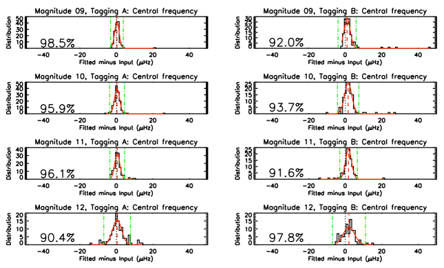
Figure 1: Histograms of the frequency differences between fits and inputs for the $l=0$ modes in the case of the 93-day Pancho time series, with a slow rotation and an inclination angle of $60^{\circ}$. The red solid lines correspond to the fitted Gaussian function to the distribution, and the dashed red lines to the mean of the distribution. The black dotted lines correspond to a difference (fits – inputs) equal to 0, while the green dashed lines represent the 3$\sigma$ limit ($\sigma$ = standard deviation of the gaussian distribution). The percentages of good fits within the 3$\sigma$ limit are also given.

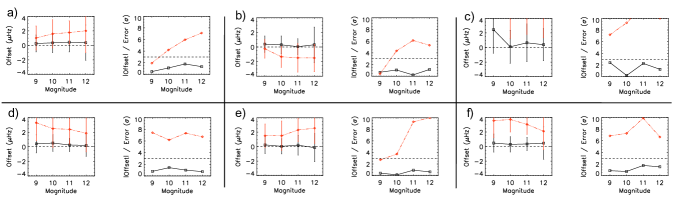
Figure 2: Offsets between the fitted and input frequencies in $\mu$Hz (left panels of a), b), c), d), e), and f)) and in sigma unit (right panels of a), b), c), d), e), and f)) as a function of the stellar magnitude M_v. The following cases are illustrated: a) $l=0$, slow rotation, angle $60^{\circ}$; b) $l=1$, slow rotation, angle $60^{\circ}$; c) $l=2$, slow rotation, angle $60^{\circ}$; d) $l=0$, fast rotation, angle $60^{\circ}$, e) $l=0$, slow rotation, angle $60^{\circ}$, Bayesian conditions; f) $l=0$, fast rotation, angle $60^{\circ}$, Bayesian conditions. The results for the correct tagging (a) and the incorrect tagging (b) are represented with black squares and red diamonds respectively.

While most of the fits fall within the 3$\sigma$ limit, clear offsets between the fitted and input frequencies are present when the incorrect tagging (b) is chosen (Fig. 2). These offsets of a few $\mu$Hz are larger than 3$\sigma_{f}$ ($\sigma_{f}$ = $\langle$formal errors$\rangle$) and tend to increase with stellar magnitude. When the correct tagging (a) is chosen, these offsets are minimal and are within the 3$\sigma_{f}$ limit.

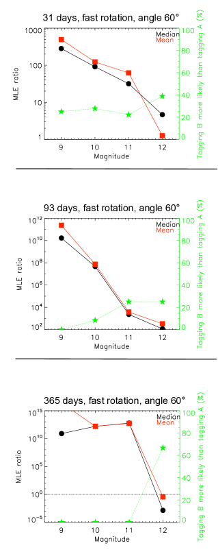
Figure 3: Likelihood ratios between the correct (a) and incorrect (b) mode identifications over the entire set of analyzed power spectra as a function of the star magnitude M_v and the length of observations $T$ (from top to bottom, $T$ = 31, 93, and 365 days respectively) for an inclination angle of $60^{\circ}$. Both mean (red squares) and median (black dots) values of the likelihood ratios are shown. The percentages that the likelihood-ratio test returns the incorrect tagging (b) as being more likely are given using the right $y$-axis (green stars).

4 Likelihood-ratio test

We present here the reliability of the likelihood-ratio test as a function of the star magnitude M_v and of the length of the observations $T$. The following discussion concerns the AsteroFLAG star Pancho with fast rotation ($5\mu$Hz) and an inclination angle of $60^{\circ}$. For the 3 lengths of observations ($T$ = 31, 93, and 365 days), Fig. 3 shows the mean and the median values of the likelihood ratios between the correct (a) and incorrect (b) mode identifications over the entire set of analyzed power spectra as a function of M_v. The percentages that the likelihood-ratio test returns the incorrect tagging (b) as being more likely are also represented (right $y$-axis). A clear dependence with M_v and $T$ is identifiable. For the same star and as the length of the time series increases, the likelihood-ratio test is more likely to return the correct answer. However, as the magnitude of the star increases, the likelihood-ratio test is not as reliable.

The percentages that the likelihood-ratio test returns the incorrect tagging (green curves on Fig 3) are:

• 31-day time series: $\sim$  25% up to M_v = 11;

• 93-day time series: $\leq$ 25% up to M_v = 12;

• 365-day time series: 0% up to M_v = 11.

In the case of stars with slow rotation, these percentages get larger, with for instance, 25% chance that the likelihood-ratio test returns the incorrect mode identification as being more likely for M_v = 9 and $T$ = 93 days. The introduction of Bayesian conditions can help mainly when the characteristics of the star make the mode identification difficult, for example, a star with slow rotation.

5 Conclusions

The identification of the oscillations modes (or mode tagging) is a necessary step before we can infer the physical properties of the star interiors. Even when using global peak-fitting techniques, the mode tagging remains a difficult task to achieve, when for instance, a large number of oscillation modes are observed with a low signal-to-noise ratio. The likelihood-ratio test can help to discriminate between the possible scenarios (i.e. taggings) and it has been already successfully applied in asteroseismology with the CoRoT, Kepler, and Procyon observations. Nevertheless, by analyzing the AsteroFLAG artificial star Pancho, we showed in this work that the likelihood-ratio test has certain limits depending on both the star magnitude and the length of the observations. For example, for a star with a rotational splitting of $5\mu$Hz and an inclination angle of $60^{\circ}$, observed during 31 days, the likelihood-ratio test will statistically return the incorrect mode identification 25% of the time for a star magnitude up to M_v = 11. This percentage decreases as the length of observation increases and for time series of 365 days, the likelihood-ratio test will return 100% of the time the correct identification up to M_v=11. However, for stars with slow rotation, the likelihood-ratio test is more likely to return the incorrect mode tagging. The use of Bayesian conditions help mostly when the star characteristics (for example, slow rotation) make the mode identification difficult.

With the long-term observations that will be collected by the Kepler mission, we hope to have enough signal-to-noise ratio to unambiguously determine the correct identification of the modes for both solar-like stars (Chaplin et al. 2010) and red giants (Bedding et al. 2010a), as well as the stars in open clusters (Stello et al. 2010). However the relative faintness of these later stars will probably require the use of the likelihood-ratio test to disentangle between the tagging of the modes.