Homogenization of nonlocal wire metamaterial via a renormalization approach

Résumé

It is well known that defining a local refractive index for a metamaterial requires that the wavelength be large with respect to the scale of its microscopic structure (generally the period). However, the converse does not hold. There are simple structures, such as the infinite, perfectly conducting wire medium, which remain non-local for arbitrarily large wavelength-to-period ratios. In this work we extend these results to the more realistic and relevant case of finite wire media with finite conductivity. In the quasi-static regime the metamaterial is described by a non-local permittivity which is obtained analytically using a two-scale renormalization approach. Its accuracy is tested and confirmed numerically via full vector 3D finite element calculations. Moreover, finite wire media exhibit large absorption with small reflection, while their low fill factor allows considerable freedom to control other characteristics of the metamaterial such as its mechanical, thermal or chemical robustness.

The effective medium theory of artificial metallo-dielectric structures goes back to the beginning of the 20th century, with the work of Maxwell-Garnett Maxwell-Garnett1904 and Wiener Wiener1912 . These, and subsequent effective medium theories focused on disordered media where only partial information on the microscopic structure was available. A major step forward was made with the work of Kock, in the 1940s Kock1948 . This time Lorentz theory Lorentz1902 ; Lorentz1916 was used to design artificial effective media, in a bottom up fashion, as an array of scatterers. In the 1970s more mathematically sophisticated methods emerged, where instead of seeking a limiting effective medium (equivalent in some suitably defined sense to the structure of interest), one obtains a limiting equation system Bensoussan1978 ; Guenneau2000 , for the macroscopic electromagnetic field in a given structure Felbacq1997 ; Bouchitte2004 ; Felbacq2005 ; Bouchitte2009 .

In recent years, the advent of negative index metamaterials and composites has led to increased interest in effective medium theories. The most popular by far is of course the Lorentz theory approach, it being the most accessible and intuitively appealing Elser2006 . However, the usefulness of Lorentz theory is much diminished when one is interested in materials where the size of objects is much larger than the distances separating them, or materials which are strongly non-local, or in which the scatterers are strongly coupled, leading to behavior of a collective nature Cabuz2008 ; Cabuz2007a . Contrary to common intuition, non-local behavior persists, in certain structures, even when the wavelength is much larger than the characteristic scale of the structure; an excellent example is the wire medium studied by Belov et al. Belov2002 ; Belov2003 ; Simovski2004a . In these situations the Lorentz model is no longer useful and more sophisticated techniques are required.

In this work we test and illustrate, for the first time, an effective medium model of the finite conductivity finite wire medium (the “bed-of-nails” structure, Fig. 1) based on a two-scale renormalization approach. Instead of letting the wavelength tend to infinity, as customary in effective medium theories, we keep it fixed, and let other geometrical parameters tend to zero. The advantage of this approach is that it leaves us the possibility of keeping some of the geometrical parameters fixed (in this case the wire length $L$), leading to a new type of partial homogenization scheme. To put it less formally, we would like to homogenize while keeping the thickness fixed with respect to the wavelength, which prevents us from letting $\lambda$ tend to infinity, so the only remaining option is to make all the other dimensions (the wire radius $r$ and the period $d$) tend to zero.

Unlike common practice in much of the metamaterials literature, we include a detailed discussion of the model’s domain of applicability, so that an engineer may be able to quickly and efficiently decide whether this kind of structure may be useful for a given purpose.

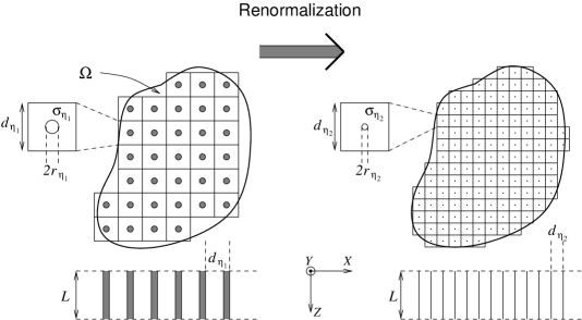
Figure 1: The bed-of-nails structure and the renormalization process. The conducting fibers occupy a region $\Omega\subseteqq\mathbb{R}^{2}$, are oriented in the $z$ direction, and the structure is periodic in the $xy$ plane. Two renormalized structures are shown, corresponding to $\eta_{1}$ and $\eta_{2}$ respectively, with $\eta_{1}>\eta_{2}$, $d_{\eta_{1}}>d_{\eta_{2}}$, $\sigma_{\eta_{1}}<\sigma_{\eta_{2}}$ and $r_{\eta_{1}}/d_{\eta_{1}}>r_{\eta_{2}}/d_{\eta_{2}}$ (see Eqs. 1 and 2). The real physical structure corresponds by definition to $\eta=1$: $d_{\eta=1}=d$. The length $L$ and the wavelength $\lambda$ remain fixed, i.e., we are homogenizing in the $xy$ plane only.

The structure under study is a square biperiodic array of thin wires, of length $L$, radius $r$ and conductivity $\sigma$. We note the period $d$ and the wavelength $\lambda$. The renormalization (depicted in Fig. 1) involves a limiting process whereby the three quantities: $r$, $d$ and $1/\sigma$ tend simultaneously to zero. The parameter governing the limiting process is noted $\eta=d$, the period. The asymptotics of the other two parameters, $\sigma$ and $r$, with respect to $\eta$ are described by fixed parameters $\kappa$ and $\gamma$ according to the following relations:

$$\kappa = \frac{\pi r_{\eta}^{2}\sigma_{\eta}}{\varepsilon_{0}\omega\eta^{2}}$$ (1)

$$\frac{1}{\gamma} = \eta^{2}\log(\frac{r_{\eta}}{\eta})$$ (2)

where $\omega$ is the angular frequency of the electromagnetic field. In other words the conductivity is renormalized inversely to the fill factor $\theta_{\eta}=\frac{\pi r_{\eta}^{2}}{\eta^{2}}$, while the radius is renormalized such that the expression $\eta^{2}\log(\frac{r_{\eta}}{\eta})$ remains constant.

While these expressions may at first seem obscure, they have simple intuitive interpretations. The first requires the current density to remain constant during the renormalization. Notice that $\kappa$ is nothing other than the volume average of the imaginary part of the permittivity. Also, recall that the static admittance per unit length of a circular wire is given by

$$Y_{\mbox{wire}} = \pi r^{2}\sigma$$ (3)

and that the number of wires per unit area is given by $1/\eta^{2}$. The second expression requires the average internal capacitance of the wires to remain constant during renormalization. This feature is known to be essential for their asymptotic behavior (see, for instance Refs. Pendry1996 ; Pendry1998 ). One may object that the expression on the right side of Eq. 2 is valid for infinitely long wires, whereas we are working with wires of finite length. Indeed, as shown below, the model fails for short wires (comparable to the period), but that configuration is best treated with the Lorentz approach anyway Collin1991 , placing it outside our present scope.

The essential quantities in the rescaling process are therefore the geometric quantities $r_{\eta}$, $\eta$, the material quantity $\sigma_{\eta}$ and the field quantities $E_{\eta}$ and $H_{\eta}.$ To these one must also add a quantity characterizing the all important electric field in the wires. This is noted $F_{\eta}$, it is non-zero only inside the wires, and is given by

$$F_{\eta} = \frac{\kappa}{\theta_{\eta}}E_{\eta}$$

$$= \frac{\sigma_{\eta}}{\varepsilon_{0}\omega}E_{\eta}.$$

$F_{\eta}$ has the units of electric field, and in the microscopic, inhomogeneous picture it is clearly proportional to the current density. In the macroscopic, homogeneous picture, however, it will correspond to the polarization density $P$. More precisely we have $\lim_{\eta\rightarrow 0}F_{\eta}=P/i\varepsilon_{0}$.

The question to be answered now becomes: what happens in the limit $\eta\rightarrow 0$ ? The answer is that the fields converge (in a precise sense described in Ref. Bouchitte2006 ) to the unique solution of the following system:

$$\begin{cases}\nabla\times E&=i\omega\mu_{0}H\\ \nabla\times H&=-i\omega\varepsilon_{0}(E+\frac{P}{\varepsilon_{0}}\hat{z})\\ \frac{\partial^{2}P_{z}}{\partial z^{2}}+\left(k_{0}^{2}+\frac{2i\pi\gamma}{\kappa}\right)P_{z}&=-2\pi\gamma\varepsilon_{0}E_{z},\,z\in[-L/2,L/2]\\ \frac{\partial P_{z}}{\partial z}&=0,\,z\in\{-L/2,L/2\}\end{cases}$$ (4)

Before solving the system, let us first see what it tells us on a more intuitive level.

All field quantities above are effective, homogeneous quantities, which have meaning when the wires have been replaced with a homogeneous effective medium with an electric polarization density equal to $P$. The equation which gives $P$ is an inhomogeneous Helmholtz equation where the source term is given by the $z$ component of the electric field $E_{z}$. The polarization satisfies Neumann conditions at the upper and lower interfaces of the slab. It is not in general continuous there because Maxwell’s equations impose the continuity of the normal component of the displacement field $D\equiv\varepsilon_{0}E+P$; consequently, any jump in $E$ must be canceled by an equivalent jump in $P/\varepsilon_{0}$. The dependence of $P$ on $E$, i.e., the constitutive relation, takes the form of an integral. In this case we are dealing with a one-dimensional inhomogeneous Helmholtz equation, but this situation is slightly complicated by the fact that it is valid on a bounded domain only (the thickness $L$ of the slab). The polarization field has the form

$$P(x,z_{0})=-2\pi\gamma\varepsilon_{0}\int_{-L/2}^{L/2}g(z,z_{0})E_{z}(x,z)dz$$ (5)

where $g(z,z_{0})$ is the Green function of the Helmholtz operator on the bounded domain $z\in\left(-\frac{L}{2},\frac{L}{2}\right)$. It takes the form (see Appendix A)

$$g(z,z_{0})=\frac{1}{K\sin(KL)}\cos\left[K(z_{<}+\frac{L}{2})\right]\cos\left[K(z_{>}-\frac{L}{2})\right]$$

where $K^{2}=k_{0}^{2}+\frac{2i\pi\gamma}{\kappa}$, $z_{<}=\min(z,z_{0})$ and $z_{>}=\max(z,z_{0})$. Relation 5 is clearly a non-local constitutive relation because the value of the polarization field at a position $z_{0}$ depends on values of the electric field at positions different from $z_{0}$.

When the imaginary part of $K$ is large the integral above drops off quickly. In the limit of small conductivity (and hence small $\kappa$), the polarization becomes local for sufficiently large wavelengths. In the opposite limit, for infinite conductivity and infinitely long wires the integral covers all space (in the $z$ direction) and the material is non-local, even in the long-wavelength regime. In fact this can be seen immediately by doing a Fourier transform on the third equation of system 4 (with $\kappa\rightarrow\infty$):

$$\widehat{P_{z}}=\frac{-2\pi\gamma\varepsilon_{0}}{k_{z}^{2}-k_{0}^{2}}\widehat{E_{z}}$$

which gives

$$\varepsilon=1+\frac{2\pi\gamma}{k_{0}^{2}-k_{z}^{2}}$$

This is consistent with the findings of Belov et al. Belov2002 ; Belov2003 ; Simovski2004a .

Until now, the discussion has been independent of the actual shape of the domain $\Omega$ (Fig. 1). From this point on, however, for purposes of illustration we specialize to the case $\Omega=\mathbb{R}^{2}$, which is an infinite two dimensional bed-of-nails, of thickness $L$, period $d$, wire radius $r$ and conductivity $\sigma$. The effective medium is therefore a homogeneous slab parallel to the $xy$ plane and of thickness $L$.

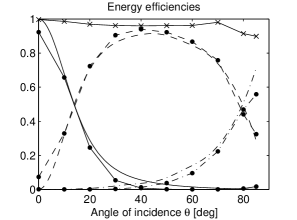
Figure 2: Transmission (solid), reflection (dot-dashed) and absorption (dashed) efficiency curves comparing the finite element solution (dot markers) and the effective medium solution (no markers) as a function of angle of incidence. The structure has a conductivity $\sigma=8(\mbox{$\Omega$m})^{-1}$, period $d=0.01\mbox{m}$, and dimensionless parameters $L/d=120$, $\lambda/d=20$, $r/d=0.1$, and $\delta/d=4.6$. Computational constraints forced us to use a very coarse mesh, which explains the approximate nature of the energy conservation ($\times$ markers) of the finite element model.

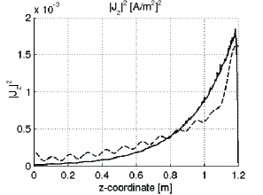
Figure 3: Square of the current density for the effective medium solution of Eqs. 9 (dashed) and the finite element solution (solid) as a function of position within the bed-of-nails structure (which is positioned in $z\in(0,L)$). The structure is the same as in Fig. 2, illuminated at an angle of incidence $\theta=40\text{\textdegree}$ from the top.

Numerical results

We now proceed to test the homogeneous model by comparing it with 3D full vector simulations of the structure, i.e. we must compare the reflection, transmission and absorption coefficients and the current distribution of the homogeneous problem with those of the original bed-of-nails metamaterial. The solution to the homogeneous problem is obtained by integrating system 4 as described in Appendix B.

The 3D full vector simulations of the bed-of-nails metamaterial were done using the Comsol Multiphysics finite element method Dular1995 software package. The periodicity was implemented using Floquet-Bloch conditions Nicolet2004 in the two periodic directions ($x$ and $y$), and absorbing Perfectly Matched Layers Agha2008 in the positive and negative $z$ directions. The linearity of the materials in the structure was used to treat the incident field as a localised source within the obstacle, as detailed in Ref. Demesy2007 ; Demesy2009a . The Comsol/Matlab scripts of the models used to produce the figures below are available as online support material for the readers’ convenience.

Figures 2 and 3 show good agreement between the effective medium model and the finite element simulation. Note that the current density behavior near the boundaries differs between the effective medium model and the finite element model. This is due to the fact that in the macroscopic, homogeneous scenario, one speaks of a polarization field obeying Neumann boundary conditions, as discussed above. In the microscopic scenario however, we have a free conductor carrying current induced by an external electric field. Since in our geometry at the given wavelength the capacitance of the wire endpoints is very small, the accumulation of charge will be correspondingly small, leading to an almost continuous normal component of the electric field (and therefore also current). Numerically, it seems as if the current goes to zero at the wire endpoints, even though this is not strictly exact. Nevertheless, since in the homogeneous limit the boundary condition of the current is of Neumann type, the convergence of the renormalization process is clearly non-uniform near the boundaries. This provides an additional explanation for requiring long wires; we want the effect of the boundaries to be small.

It must also be pointed out that the parameters of the particular structure chosen for the illustration in Figs. 2 and 3 were forced upon us by practical constraints: finite element meshing of thin long circular wires requires very large amounts of computer memory and time. Simulation of wires thinner than $r/d=0.05$ is prohibitive. Consequently, in order to explore a wider domain of the parameter space, we have taken advantage of the fact that the structures we are interested in have $r\ll d$ and $\delta\gg r$. Such thin conducting structures can be simulated much more efficiently as lines of zero thickness Carpes2002 (i.e. edges, in the finite element formulation) carying current and exhibiting an equivalent linear impedance. This approach gives excellent results with a fraction of the computing power, and enables us to model realistic structures that would otherwise be inaccessible.

For instance, Figs. 4 and 5 show the results of calculations for a structure of Toray T300^®carbon fibers Toray with a conductivity of: $\sigma=5.89\cdot 10^{4}(\mbox{$\Omega$m})^{-1}$ and a radius of $3.5$ microns. The wires have an aspect ratio $L/r=2.28\times 10^{5}$, which is far beyond what would have been accessible by meshing the interior of the wires. The finite element model of Fig. 2 (curves with markers), in which the interior of the wires is meshed, is a problem with approx. 2.8 million degrees of freedom, which requires at least 42 Gigabytes of available RAM to solve. By comparison, the model of Fig. 4 (curves with markers), in which the wires are modeled as current carrying edges, is a problem of approx. 62 thousand degrees of freedom, which requires less than one Gigabyte of available RAM and can therefore be solved on any sufficiently recent desktop computer.

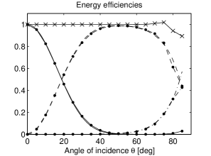
Figure 4: Transmission (solid), reflection (dot-dashed) and absorption (dashed) efficiency curves comparing the finite element solution (dot markers) and the effective medium (no markers) as a function of angle of incidence. The wire conductivity is that of Toray T300^® carbon fibers $\sigma=5.89\cdot 10^{4}(\mbox{$\Omega$m})^{-1}$. The structure has period $d=0.01\mbox{m}$, and dimensionless parameters $L/d=80$, $\lambda/d=20$, $r/d=3.5\cdot 10^{-4}$, and $\delta/r=15$. Energy conservation of the finite element model ($\times$ markers) is respected to within better than one percent for most angles of incidence. The departure around 80° is explained by the poor performance of the PML absorbing layers when close to grazing incidence.

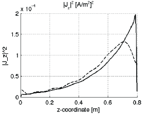
Figure 5: Square of the current density for the effective medium model (dashed) and the finite element solution (solid) as a function of position within the slab (which is positioned in $z\in(0,L)$). The structure is the same as in Fig. 4, illuminated at an angle of incidence $\theta=40\text{\textdegree}$ from the top. Note that the surface areas under the two curves (in this figure as well as Fig. 3) are the same because they are proportional to the Joule dissipation rates, which are seen to be equal from Fig. 4 (and Fig. 2) at the given angle of incidence.

Figures 2, 3, 4, and 5 illustrate the behavior which is typical of the model. The agreement remains good up to high incidence angles, and over a large wavelength domain (Fig. 7). The structure is transparent in normal incidence. For increasingly oblique angles of incidence the absorption increases more or less gradually, depending on the thickness $L$. The reflection is generally low, though it increases when approaching grazing incidence. The low reflection may be explained by the small radii of the wires: their extremities have low capacitance, hence they exhibit very little charge accumulation, leading to an almost continuous normal component of the electric field. Certain configurations exhibit very low reflection for almost all angles of incidence, see Fig. 6

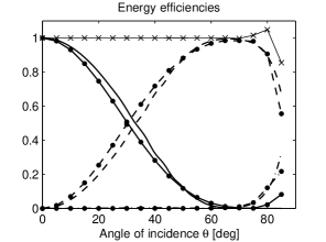
Figure 6: Transmission (solid), reflection (dot-dashed) and absorption (dashed) efficiency curves comparing the finite element solution (dot markers) and the effective medium (no markers) as a function of angle of incidence. The structure has a conductivity $\sigma=1000(\mbox{$\Omega$m})^{-1}$, period $d=0.01\mbox{m}$, and dimensionless parameters $L/d=50$, $\lambda/d=8$, $r/d=0.002$, and $\delta/d=13$. The reflection remains low for angles of incidence of up to 80° even as the Joule absorption reaches almost 100% for $\theta>60\text{\textdegree}$. Energy conservation is indicated by the $\times$ markers.

and Fig. 7 around $\lambda=1.2\mbox{m}$. The current density decreases roughly exponentially within the structure due to absorption.

Domain of validity

The boundaries of the domain of validity of the model are given by four dimensionless parameters: the ratio of the skin depth to the radius in the wires $\delta/r$, the ratio of the wire length to the period $L/d$, the ratio of the wavelength to the period $\lambda/d$ and the ratio of the wire radius to the period $r/d$.

The skin depth must be larger than the radius, due to the fact that the impedance used in defining $\kappa$ (Eq. 3) is the static impedance which differs from the quasistatic value by an imaginary inductive term $i\omega\mu/8\pi$ (see, for instance, Ref. Ramo1994 ). Requiring this term to be negligible is equivalent to requiring that $\delta^{2}/r^{2}\gg 1$. Moreover, in the rescaling process the skindepth/radius ratio is given by

$$\frac{\delta_{\eta}}{r_{\eta}}=\frac{\lambda}{\eta}\sqrt{\frac{1}{2\pi\kappa}}.$$

Since $\eta$ approaches zero in the rescaling process, it is natural to expect the homogeneous model to be valid when the skindepth is large compared to the radius.

In addition, recall that the definition of $\gamma$ in Eq. 2 fixes the capacitance of the wires to the value for thin, long wires. Consequently, we expect the model to hold for large $L/d$ and for small $r/d$. To these, we must add the general requirement for all effective medium models: the wavelength must be large compared to the period.

Due to the large (four dimensional) parameter space, an exhaustive numerical exploration of the bed-of-nails structure is not feasible in a reasonable timeframe. Still, our study has made it possible to broadly determine the boundaries of the domain of applicability of the effective medium model. Roughly, one must have $\lambda/d\gtrapprox 7-12$, $\delta/r\gtrapprox 4-8$, $L/d\gtrapprox 20-30$, $r/d\lessapprox 10$. Our (a fortiori limited) numerical exploration of the parameter space suggests that the skindepth-to-radius ratio is often the main limiting factor, particularly when considering highly conducting wires.

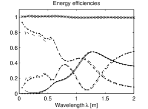
Figure 7: Transmission (solid), reflection (dot-dashed) and absorption (dashed) efficiency curves comparing the finite element solution (dot markers) and the effective medium (no markers) as a function of wavelength. Energy conservation for the finite element model is labeled with $\times$ markers. The structure has a conductivity $\sigma=3000(\mbox{$\Omega$m})^{-1}$ (in the semiconductor domain), period $d=0.01\mbox{m}$, and dimensionless parameters $L/d=60$, $r/d=0.003$, and the angle of incidence is $\theta=70\text{\textdegree}$. $\delta/r$ runs approximately from $4$ to $25$ from left to right over the domain of the plot. The model fails around $\lambda\lessapprox 0.1\mbox{m}=10d$.

Conclusion

We have tested numerically the effective medium theory of the bed-of-nails structure, whose rigorous mathematical foundation is described in Ref. Bouchitte2006 . We have found good agreement between the transmission, reflection and absorption efficiencies between the effective medium model and a 3D finite element model, for a broad range of angles of incidence and wavelengths. The current density in the real structure corresponds to the polarization current density of the effective medium model. The medium is nonlocal, meaning that the polarization field depends on the electric field over a region of finite size. That dependence is given by Eq. 5. This nonlocal behavior also means that the permittivity depends on the wavevector, so it can no longer be seen, strictly, as a property of the medium, but rather, as a property of a given wave propagating in the structure Menzel2008 ; Rockstuhl2008 .

The bed-of-nails structure is a medium exhibiting high absorption with low reflection. It requires a very low filling fraction of conducting material, but exhibits near perfect absorption over a wide range of angles of incidence, for sufficiently large thicknesses. The low filling fraction is useful because it allows the engineer to fill the space between the wires with materials satisfying other design constraints, such as mass density, or mechanical, chemical or thermal robustness. The geometries studied here are transparent at normal incidence, but this aspect can easily be rectified by slanting the wires by about 20° with respect to the upper and lower boundaries. This design may therefore be used to obtain a near-perfect electromagnetic absorber for all angles of incidence in a very straightforward way, and with considerable freedom in the resulting mechanical, thermal or chemical properties of the structure. We are currently exploring more elaborate structures which may be modeled by the same scaling technique: structures with thin wires in the x and/or y directions as well as the z direction, or with wires curved helically, leading to a non-trivial magnetic constitutive relation in addition to the electric one.

Appendix A

We require the Green function for the problem (see chapter II of Ref. Schwartz2009 )

$$p^{{}^{\prime\prime}}+\alpha^{2}p=\beta E_{z}$$

with

$$p^{{}^{\prime}}(-L/2)=p^{{}^{\prime}}(L/2)=0.$$ (6)

For the purpose of this Appendix it is convenient to consider the structure is positioned between$-L/2$ and $L/2$. The Green function satisfies the equation

$$g^{{}^{\prime\prime}}+\alpha^{2}g=\delta_{z_{0}} z_{0}\in\left(-\frac{L}{2},\frac{L}{2}\right)$$ , (7)

and may be written:

$$g(z,z_{0}) = Cu_{1}(z_{<})u_{2}(z_{>})$$

with

$$z_{<} = \min(z,z_{0})$$

$$z_{>} = \max(z,z_{0})$$

such that

$$\mbox{when }z\in\left(-\frac{L}{2},z_{0}\right) g=Cu_{1}(z)u_{2}(z_{0})$$ ,

and

$$\mbox{when }z\in\left(z_{0},\frac{L}{2}\right) g=Cu_{1}(z_{0})u_{2}(z)$$ ,

Replacing form Appendix A into Eq. 7 one obtains that $g$ must be continuous at $z_{0}$, its derivative must have a jump discontinuity of 1, and the two functions $u_{1}$ and $u_{2}$ must be sinusoidal of wave constant $\alpha$:

$$u_{1}(z) = A\cos(\alpha(z+L/2))$$

$$u_{2}(z) = B\cos(\alpha(z-L/2)).$$

By imposing the boundary conditions Eq. 6 we obtain

$$u_{1}^{{}^{\prime}}(-L/2) = 0$$

$$u_{2}^{{}^{\prime}}(L/2) = 0$$

and by requiring a jump discontinuity of 1 at $z_{0}$ we obtain

$$ABC=\frac{1}{\alpha\sin(\alpha L)}$$

giving finally:

$$g(z,z_{0})=\frac{1}{\alpha\sin(\alpha L)}\cos(\alpha(z_{<}+L/2))\cos(\alpha(z_{>}-L/2))$$

Appendix B

We now proceed to solve the homogeneous limit system 4. For convenience we position it in $z\in(0,L)$. Since we are dealing with a system with translational invariance, a slab, we can split the problem into two independent polarization cases: TE, where the electric field is in the $xy$ plane, and TM, where the magnetic field is in the $xy$ plane. However, since we are considering thin wires (small volume fraction) the structure will be transparent to TE waves. We therefore only have to consider TM waves. We choose a coordinate system so that the plane of incidence is the $xz$ plane, with angle of incidence $\theta$, in which case our unknowns will be $H_{y}$ and $P_{z}$. The translation invariance allows us to seek solutions of the form:

$$H_{y} = u(z)e^{i\alpha x}$$

$$P_{z} = p(z)e^{i\alpha x}$$

with: $\alpha=k_{0}\sin\theta$. Inserting these into system 4 we obtain a system of equations for $u$ and $p$:

$$\begin{cases}u^{\prime\prime}(z)+\left(k_{0}^{2}-\alpha^{2}\right)u(z)&=\alpha\omega p(z)\\ p^{\prime\prime}(z)+\left(k_{0}^{2}+\frac{2i\pi\gamma}{\kappa}-2\pi\gamma\right)p(z)&=\frac{2\pi\alpha\gamma}{\omega}u(z),\,z\in[0,L]\end{cases}$$ (9)

with the important boundary conditions: $p^{\prime}=0$ at $z=0$ and $z=L$, and $u$ and $u^{\prime}$ continuous everywhere.

The objective is now to obtain the transfer matrix $T$ of the slab, which relates the field $u$ and its derivative $u^{\prime}$ at the bottom and the top of the slab:

$$\left(\begin{array}[]{c}u(L)\\ u^{\prime}(L)\end{array}\right)=T\left(\begin{array}[]{c}u(0)\\ u^{\prime}(0)\end{array}\right).$$ (10)

Once $T$ is known the reflection and transmission coefficients $r$ and $t$ can be obtained immediately from

$$r=e^{-2i\beta L}\frac{A+B}{A-B} t=\frac{2e^{-i\beta L}}{A-B}$$ and (11)

$$A\equiv T_{11}-i\beta T_{12} B\equiv\frac{T_{21}-i\beta T_{22}}{i\beta}$$ and

where $\beta=k_{0}\cos\theta=\sqrt{k_{0}^{2}-\alpha^{2}}$.

We begin by integrating system 9. Noting $\delta^{2}=k_{0}^{2}+\frac{2i\pi\gamma}{\kappa}-2\pi\gamma$ for readability, we rewrite the system as

$$W^{\prime\prime}(z) = -MW(z)$$ (12)

where

$$W(z)=\left(\begin{array}[]{c}u(z)\\ p(z)\end{array}\right)$$

and

$$M=\left(\begin{array}[]{cc}\beta^{2}&-\alpha\omega\\ -\frac{2\pi\alpha\gamma}{\omega}&\delta^{2}\end{array}\right).$$

The matrix $M$ can be diagonalized $M=QDQ^{-1}$ with $D=\mbox{diag}(K_{u}^{2},K_{p}^{2})$ so the system 12 can be rewritten $Q^{-1}W^{\prime\prime}(z)=-DQ^{-1}W(z)$. Since $Q$ is constant and known, this can be integrated directly, and the general solution is then obtained as a sum of plane waves:

$$Q^{-1}W(z)=\left(\begin{array}[]{c}A_{u}^{+}\exp(iK_{u}z)+A_{u}^{-}\exp(-iK_{u}z)\\ A_{p}^{+}\exp(iK_{p}z)+A_{p}^{-}\exp(-iK_{p}z)\end{array}\right)$$ (15)

Once the integration performed, obtaining $T$ is now only a matter of algebraic manipulation. $u$ and $p$ are now expressed in terms of the elements of the matrix $Q$ and the coefficients $A_{u}^{+}$, $A_{u}^{-}$, $A_{p}^{+}$ and $A_{p}^{-}$. However, recall that we are not interested directly in these coefficients, but in the matrix $T$. Since that matrix does not depend directly on $p$ the first step is to eliminate the $A_{p}$s from the equation system. This is done by making use of the boundary conditions. By differentiating the bottom equation of system 15 we can obtain $p^{\prime}$ as

$$p^{\prime} = iK_{u}Q_{21}(A_{u}^{+}e^{iK_{u}z}-A_{u}^{-}e^{-iK_{u}z})$$

$$+iK_{p}Q_{22}(A_{p}^{+}e^{iK_{p}z}-A_{p}^{-}e^{-iK_{p}z}).$$

Setting this to zero at $z=0,L$ we can obtain the $A_{p}$s in terms of the $A_{u}$s. Noting vectors

$$\underline{A_{u}} = \left(\begin{array}[]{c}A_{u}^{+}\\ A_{u}^{-}\end{array}\right)$$

$$\underline{A_{p}} = \left(\begin{array}[]{c}A_{p}^{+}\\ A_{p}^{-}\end{array}\right),$$

we introduce the matrix

$$C = -\frac{K_{u}Q_{21}}{K_{p}Q_{22}}\frac{1}{2i\sin(K_{p}L)}$$

$$\times\left(\begin{array}[]{cc}e^{iK_{u}L}-e^{-iK_{p}L}&e^{-iK_{p}L}-e^{-iK_{u}L}\\ e^{iK_{u}L}-e^{iK_{p}L}&e^{iK_{p}L}-e^{-iK_{u}L}\end{array}\right)$$

so that

$$\underline{A_{p}}=C\underline{A_{u}}.$$

We are now in a position to express $W(z)$ in terms of $\underline{A_{u}}$ alone. Eq. 15 can be rewritten

$$W(z)=QE(z)\underline{A_{u}}$$ (19)

where $E(z)$ is defined as

$$E(z)=\left(\begin{array}[]{cc}e^{iK_{u}z}&e^{-iK_{u}z}\\ C_{11}e^{iK_{p}z}+C_{21}e^{-iK_{p}z}&C_{12}e^{iK_{p}z}+C_{22}e^{-iK_{p}z}\end{array}\right).$$

Eq. 19 contains (within its first row) the expression for $u$. But to obtain the transfer matrix $T$ we also require $u^{\prime}$. We simply differentiate Eq. 19 to obtain

$$W^{\prime}(z)=QE^{\prime}(z)\underline{A_{u}}.$$ (20)

By combining the first rows of Eqs. 19 and 20, we are in a position to construct the matrix $G(z)$ such that

$$\left(\begin{array}[]{c}u(z)\\ u^{\prime}(z)\end{array}\right)=G(z)\underline{A_{u}}.$$

By writing this equation at $z=0$ and $z=L$ we obtain

$$\left(\begin{array}[]{c}u(z)\\ u^{\prime}(z)\end{array}\right)=G(L)G(0)^{-1}\left(\begin{array}[]{c}u(0)\\ u^{\prime}(0)\end{array}\right).$$

Comparing with Eq. 10 we obtain the result we seek,

$$T=G(L)G(0)^{-1},$$

leading to the reflection and transmission coefficients via Eqs. 11. The Matlab script of the above manipulations is available as online support material for the readers’ convenience.

To summarize, we are now capable of modeling a structure with a given $d$, $r$, $\sigma$, $L$ at a given incident field wavelength $\lambda$ in the following way. We first obtain the two rescaling parameters $\kappa$ and $\gamma$ for the given structure using Eqs. 1 and 2. Then, we integrate system 9 to obtain the reflection and transmission coefficients.

- (1) J. Maxwell-Garnett Phil. Trans. R. Soc. Lond. A, vol. 203, p. 385, 1904.
- (2) O. Wiener Abh. Math.-Phys. Konigl. Sachs. Ges., vol. 32, p. 509, 1912.
- (3) W. E. Kock, “Metallic delay lenses,” Bell System Technical Journal, vol. 27, no. 1, pp. 58–82, 1948.
- (4) H. Lorentz Proc. Roy. Acad., Amsterdam, vol. 254, 1902.
- (5) H. Lorentz, The theory of electrons and its applications to the phenomena of light and radiant heat. G.E. Stechert and Co., 1916.
- (6) A. Bensoussan, J. Lions, and G. Papanicolaou, Asymptotic Analysis for Periodic Structures. North-Holland, Amsterdam, 1978.
- (7) S. Guenneau and F. Zolla, “Homogenization of three-dimensional finite photonic crystals - abstract,” Journal of Electromagnetic Waves and Applications, vol. 14, no. 4, pp. 529–530, 2000.
- (8) D. Felbacq and G. Bouchitté, “Homogenization of a set of parallel fibers,” Waves in Random Media, vol. 7, pp. 245, 1997.
- (9) G. Bouchitté and D. Felbacq, “Homogenization near resonances and artificial magnetism from dielectrics,” Comptes Rendus Mathematique, vol. 339, pp. 377–382, Sept. 2004.
- (10) D. Felbacq and G. Bouchitté, “Theory of mesoscopic magnetism in photonic crystals,” Phys. Rev. Lett., vol. 94, no. 18, p. 183902, 2005.
- (11) G. Bouchitté, C. Bourel, and D. Felbacq, “Homogenization of the 3D Maxwell system near resonances and artificial magnetism,” Comptes Rendus de l’Academie des Sciences Serie I, vol. 347, p. 571, 2009.
- (12) J. Elser, R. Wangberg, V. A. Podolskiy, and E. E. Narimanov, “Nanowire metamaterials with extreme optical anisotropy,” Applied Physics Letters, vol. 89, 2006.
- (13) A. I. Căbuz, D. Felbacq, and D. Cassagne, “Spatial dispersion in negative-index composite metamaterials,” Phys. Rev. A, vol. 77, no. 1, p. 013807, 2008.
- (14) A. I. Căbuz, Electromagnetic metamaterials - From photonic crystals to negative index composites. PhD thesis, University of Montpellier II, 2007.
- (15) P. A. Belov, S. A. Tretyakov, and A. J. Viitanen, “Dispersion and reflection properties of artificial media formed by regular lattices of ideally conducting wires,” Journal of Electromagnetic Waves and Applications, vol. 16, no. 8, pp. 1153–1170, 2002.
- (16) P. A. Belov, R. Marques, S. I. Maslovski, I. S. Nefedov, M. Silveirinha, C. R. Simovski, and S. A. Tretyakov, “Strong spatial dispersion in wire media in the very large wavelength limit,” Phys. Rev. B, vol. 67, no. 11, p. 113103, 2003.
- (17) C. R. Simovski and P. A. Belov, “Low-frequency spatial dispersion in wire media,” Physical Review E, vol. 70, no. 4, p. 046616, 2004.
- (18) J. B. Pendry, A. J. Holden, W. J. Stewart, and I. Youngs, “Extremely low frequency plasmons in metallic mesostructures,” Physical Review Letters, vol. 76, no. 25, pp. 4773–4776, 1996.
- (19) J. B. Pendry, A. J. Holden, D. J. Robbins, and W. J. Stewart, “Low frequency plasmons in thin-wire structures,” J. of Phys.-Cond. Matt., vol. 10, no. 22, p. 4785, 1998.
- (20) R. E. Collin, Field theory of guided waves. IEEE Press, 1991.
- (21) G. Bouchitté and D. Felbacq, “Homogenization of a wire photonic crystal: The case of small volume fraction,” SIAM Journal On Applied Mathematics, vol. 66, no. 6, pp. 2061–2084, 2006.
- (22) P. Dular, A. Nicolet, A. Genon, and W. Legros, “A discrete sequence associated with mixed finite-elements and its gauge condition for vector potentials,” IEEE Transactions on Magnetics, vol. 31, no. 3, pp. 1356–1359, 1995.
- (23) A. Nicolet, S. Guenneau, C. Geuzaine, and F. Zolla, “Modelling of electromagnetic waves in periodic media with finite elements,” Journal of Computational and Applied Mathematics, vol. 168, no. 1-2, pp. 321–329, 2004.
- (24) Y. Ould Agha, F. Zolla, A. Nicolet, and S. Guenneau, “On the use of pml for the computation of leaky modes - an application to microstructured optical fibres,” COMPEL -The International Journal for Computation and Mathematics in Electrical and Electronic Engineering, vol. 27, no. 1, pp. 95–109, 2008.
- (25) G. Demésy, F. Zolla, A. Nicolet, M. Commandré, and C. Fossati, “The finite element method as applied to the diffraction by an anisotropic grating,” Opt. Express, vol. 15, no. 26, pp. 18089–18102, 2007.
- (26) G. Demésy, F. Zolla, A. Nicolet, and M. Commandre, “Versatile full-vectorial finite element model for crossed gratings,” Optics Letters, vol. 34, no. 14, pp. 2216–2218, 2009.
- (27) W. Carpes Jr., L. Pichon, and A. Razek, “Analysis of the coupling of an incident wave with a wire inside a cavity using fem in frequency and time domains,” IEEE Transactions on Electromagnetic Compatibility, vol. 44, p. 470, 2002.
- (28) Toray Carbon Fibers America Inc.
- (29) S. Ramo, J. R. Whinnery, and T. Van Duzer, Fields and Waves in Communication Electronics. John Wiley and Sons, third ed., 1994.
- (30) C. Menzel, C. Rockstuhl, T. Paul, F. Lederer, and T. Pertsch, “Retrieving effective parameters for metamaterials at oblique incidence,” Phys. Rev. B, vol. 77, pp. 195328–8, May 2008.
- (31) C. Rockstuhl, C. Menzel, T. Paul, T. Pertsch, and F. Lederer, “Light propagation in a fishnet metamaterial,” Physical Review B, vol. 78, p. 155102, Oct. 2008.
- (32) L. Schwartz, Mathematics for the Physical Sciences. Dover Books on Mathematics, 2009.