Time-dependent radio emission from evolving jets

Abstract

We investigated the time-dependent radiative and dynamical properties of light supersonic jets launched into an external medium, using hydrodynamic simulations and numerical radiative transfer calculations. These involved various structural models for the ambient media, with density profiles appropriate for galactic and extragalactic systems. The radiative transfer formulation took full account of emission, absorption, re-emission, Faraday rotation and Faraday conversion explicitly. High time-resolution intensity maps were generated, frame-by-frame, to track the spatial hydrodynamical and radiative properties of the evolving jets. Intensity light curves were computed via integrating spatially over the emission maps. We apply the models to jets in active galactic nuclei (AGN). From the jet simulations and the time-dependent emission calculations we derived empirical relations for the emission intensity and size for jets at various evolutionary stages. The temporal properties of jet emission are not solely consequences of intrinsic variations in the hydrodynamics and thermal properties of the jet. They also depend on the interaction between the jet and the ambient medium. The interpretation of radio jet morphology therefore needs to take account of environmental factors. Our calculations have also shown that the environmental interactions can affect specific emitting features, such as internal shocks and hotspots. Quantification of the temporal evolution and spatial distribution of these bright features, together with the derived relations between jet size and emission, would enable us to set constraints on the hydrodynamics of AGN and the structure of the ambient medium.

1 Introduction

Jets are present in astrophysical systems from active galaxies (see Begelman et al., 1984) to stellar systems, such as X-ray binaries (Hjellming & Johnston, 1981; Mirabel & Rodríguez, 1999; Fender, 2006) and symbiotic stars (Taylor et al., 1986; Sokoloski et al., 2004). They are supersonic. The jets from active galactic nuclei (AGN) are also relativistic, and they show a large variety of morphologies and properties.

Although the jet plasmas have densities orders of magnitude smaller than the density of the ambient media, the large momentum flux carried in the plasmas enable the jets to propagate great distances, even up to Mpc scales. These jets impart momentum to the ambient gas. A termination shock (which appears as a hotspot) is often formed at the jet front, but in some cases, a series of lesser shocks along its length. Shocked jet plasmas fill low-density central cocoons, comprising eddies, backflows as well as transient shocks. Internal shocks may stand or propagate along the jet itself, corresponding to intrinsic pinching modes (e.g. Hardee, 1979; Cohn, 1983; Norman et al., 1982; Hardee, 1983, 1987; Falle et al., 1987; Koessl & Mueller, 1988) or stochastic disturbances from motions of the cocoon plasma. Studies have show that the termination shock may be stable or unstable, depending on the system conditions. There are cases that the termination shock is susceptible to vortex shedding, throbbing and disintegration (e.g. Norman et al., 1982; Norman et al., 1988; Chakrabarti, 1988; Koessl & Mueller, 1988; Falle, 1991; O’Neill et al., 2005). The disrupted hotspots and shocks in the backflow may be the cause of the bright rings or filaments seen in some radio galaxies.

The energetic particles in jets emit strong synchrotron radio waves, and in some cases, synchrotron X-rays (e.g. M87, Marshall et al., 2002; Perlman & Wilson, 2005). In FR2 radio galaxies, jets tend to end in termination shocks, where the jet plasma decelerates abruptly as it encounters a dense external medium. The shocks compress the magnetic filed and convert the kinetic energy in the bulk flow into microscopic kinetic energy. In shock regions, charged particles are accelerated to relativistic speeds, giving rise to synchrotron emission. The energetic particles in the jet also upscatter the low-energy photons (from the jet itself or from the ambient radiation field) to the X-ray energy ranges. Radio synchrotron emissions from jets are linearly polarized (see e.g. Mantovani et al., 1997). Some AGN also show substantial circular polarization, in their core radio emission and in the jet knots (Hodge & Aller, 1977; Weiler & de Pater, 1983; Komesaroff et al., 1984; Homan & Wardle, 1999; Rayner et al., 2000; Aller et al., 2003; Homan & Wardle, 2004; Homan & Lister, 2006; Vitrishchak et al., 2008; Cenacchi et al., 2009). Theoretical studies (see McNamara et al., 2009) have shown that Compton scattered X-rays from jets can also be strongly polarized.

Jets are dynamical: their structures change over time. The jet evolution is manifested in morphological changes in their radio image and in their emission lightcurves. Studies on the emission properties of jets tend to adopt stationary structures. Simultaneous time-dependent radiative transfer calculations along with hydrodynamical simulations of jet evolution are rare as they are usually computationally demanding. However, only such time-dependent calculations/simulations could allow us to generate appropriate multi-wavelength lightcurve templates so to have a holistic pictures of the time-evolution of various jets (in particular, those in micro-quasars) and how they interact with the ambient media.

Here we present high time-resolution simultaneous radiative transfer calculations and hydrodynamic simulations of evolving jets in a variety of ambient media. The radiative transfer calculations are carried out frame by frame following the evolution of the jet density, velocity and thermal structures in the hydrodynamic simulations. Time-sequences of emission images and light curves of jets are computed. Our study will shed light on the time-dependent hydrodynamics and radiative properties of radio jets.

The paper is organised as follows. An introduction is given in §1; the methodology of the hydrodynamic simulations and radiative transfer calculations are laid out in §2. The emission properties of simulated jets, their interactions with ambient media, and the astrophysical implications are discussed in §3. We conclude in §4.

2 CALCULATIONS

2.1 hydrodynamic simulations

In this study, we consider supersonic jets with low density. Without losing generality, we consider axially symmetric jets. (Note that we have carried out full 3D hydrodynamic simulations for a few test cases without imposing the axi-symmetric condition. We have found that the results are quantitatively similar to the corresponding axi-symmetric cases, but the computational time for each run does not let us conduct a comprehensive survey of various jet conditions and jet-interaction with the ambient media.) There are substantial works on the properties of such jets, (e.g Norman et al., 1982; De Young, 1986; Smith et al., 1985; Rosen et al., 1999; Carvalho & O’Dea, 2002; Saxton et al., 2002; Saxton et al., 2002; Krause, 2003, 2005).

Our hydrodynamic simulations adopt the piecewise parabolic method (PPM) algorithm: an explicitly conservative, shock-capturing, grid-based numerical scheme (Colella & Woodward, 1984; Blondin & Lufkin, 1993). We the ppmlr code (Sutherland et al., 2003; Saxton et al., 2001; Saxton et al., 2005) a descendant of the standard VH-1 University of Virginia hydrocode, modified to improve numerical stability and parallelisation and to consider better tracer variables to distinguish fluids of differing origins. The computational grid consists of $600\times 300$ cells (in longitudinal and radial directions respectively). A reflecting condition applies on the cylindrical axis. Numerically, this border copies the nearby cells into corresponding ghost cells beyond the edge (with vector quantities reversed to ensure balanced restoring forces). The right boundary and the outer cylindrical boundary are open to outflow. The jet nozzle spans 15 cells radially at the left boundary. Unless otherwise stated, a constant inflow condition is applied. Outside the nozzle, the rest of the left boundary has either an “open” condition or a reflecting condition (“closed boundary”). For “open” boundary condition, we consider selective reflection to prevent inflow (if $v>0$ at a border cell). For edge outflow ($v<0$ at the edge), zero gradients (and zero force) is enforced, through copying the single boundary cell into all ghost cells. No explicit treatment of radiative cooling is in the hydrodynamics formulation. We also omit self-gravity effects. These omissions would not cause significant effects and our results generally hold, provided that the free-fall timescales are longer than the crossing times associated with supersonic motions.

In our formulation, the simulated jets are characterized by two parameters: the jet Mach number $\mathcal{M}\equiv~{}v_{\rm j}/c_{\rm s,j}$ and the density contrast $\eta\equiv\rho_{\rm j}/\rho_{\rm icm}$. Here $c_{\rm s,j}$ is the adiabatic sound speed in the jet plasma, and the subscript “icm” denotes the ambient medium. For adiabatic jets, variables such as mass, length and time can be rescaled, but the contrast variables $\eta$ and $\mathcal{M})$ are fixed parameters. Generally, the thermal velocity dispersion in the ambient medium may be used to set the velocity unit of the simulations, In this study, we consider an astrophysical realization appropriate for giant radio galaxies. The cylindrical region in the simulations spans $150{\rm kpc}\times 75{\rm kpc}$. The jet radius is about $3.75{\rm kpc}$. If we assume that the jet propagates in an intra-cluster medium (ICM) with a temperature of $10^{7}$ K and a density of $\sim 2\times 10^{-27}~{}{\rm g}~{}{\rm cm}^{-3}$ (corresponding to a particle density of $n_{\rm icm}=10^{-3}~{}{\rm cm}^{-3}$), then the velocity unit $U_{v}=365.5~{}{\rm km}~{}{\rm s}^{-1}$ and the time unit $U_{t}=10.03$ Myr.

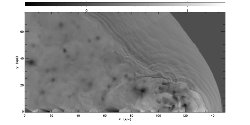
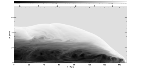
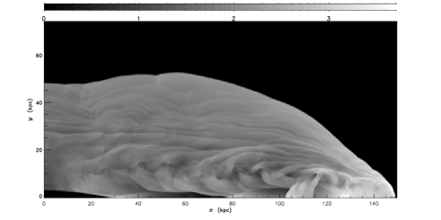
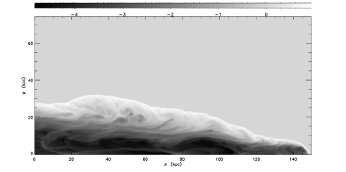
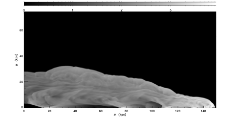
Figure 1: Sections of jet through the cylindrical structure at final frames of three simulations. The grey values and scale bar are decimal logarithmic. The jet axis runs along the bottom of each frame. The radial direction runs upwards. The left panels show the density; the right panels show the pressure (a proxy for $B^{2}/8\pi$). The slow jet is on the upper, and the fast1o jet is on the middle row. The jet plasma is a polytropic gas with $\gamma=5/3$. The fast1ro jet is on the bottom row. The simulation has the parameters and set ups same as those of the fast1o jet, except that the jet plasma is relativistic with $\gamma=4/3$.

As a basis of comparison, we first carry out simulations of jets launched into uniform media. This simple setting avoids the unnecessary complications caused by the structures in the ambient medium and enables us to identify the dynamics and emission properties intrinsic to the jets. We consider two jet models. In the first simulation (fast1o) we set $\mathcal{M}=50$ and $\eta=10^{-4}$. The corresponding particle column density through the jet is $\approx 2.3\times 10^{15}~{}{\rm cm}^{-2}$. In this case, the jets are expected to produce hotspots and other shocks with high brightness contrast relative to their surroundings (e.g. the radio galaxy Pictor A, Saxton et al., 2002). In the second simulation (slow) we consider a lower Mach number ($\mathcal{M}=3$) for the jet. The density of the ambient medium is the same. These jets tend to give lower luminous contrast for their induced features (e.g.  the radio galaxy Hercules A Saxton et al., 2002). The upper and middle rows of Figure 1 show density and pressure slices of slow and fast1o at late times.

Next we run simulations for jets propagating into media with various density structures. In the fast2 and fast2o simulations, we assume a decreasing medium density following a flat-cored model (Cavaliere & Fusco-Femiano, 1976)

$$\rho={{\rho_{0}}\over{\left[{1+(r/r_{0})^{2}}\right]^{3\xi/2}\ .}}$$ (1)

We set the parameter $\xi=0.5$ and the scale radius $r_{0}=15~{}{\rm kpc}$. Cases with a reflecting and an open left boundary are investigated. (Open cases are named with a suffix “o”.) In the fast3 simulations, we consider a model where the density of the ambient medium increases with radius. We set $\xi=-1$ and $r_{0}=15~{}{\rm kpc}$. In the fast4 simulations, the density of the ambient medium varies sinusoidally, with $\rho=\rho_{0}\ \exp[-a\sin(kr)]$, where the wavenumber $k=2\pi/\lambda_{0}$. We set the amplitude $a=\log_{e}10$. This gives an effective wavelength of the variation $\lambda_{0}=30~{}{\rm kpc}$. In the fast1r and fast1ro simulations, we investigate the effects of the equation state. The jet plasma now has an adiabatic index $\gamma=4/3$ (characteristics of relativistic gas) instead of $5/3$. Table 1 lists the principal parameters of the simulations and the temporal sequence of output frames.

Table 1: Settings and parameters of the simulations. For those marked $\CIRCLE$ the left boundary is closed/reflecting; for those marked $\Circle$ it is open. The jet density contrast and Mach number are $\eta=\rho_{\rm j}/\rho_{\rm ism}$ and $\mathcal{M}$. The duration of each simulation is $t_{\rm end}$ and the interval between frames is $\Delta t$ (both in units of $U_{t}\approx 10.03$ Myr). Runs with nonuniform ambient media have index $\xi$ and scale radius $r_{0}$. (The grid size is $40\times 20$ in the same units.) $N$ counts the frames.

$\begin{array}[]{lcrrr@{.}lrrrrrrrrrrrrrrrrrrrrrrrrrrrr}\mbox{run}&\mbox{BC}&\eta&{\mathcal{M}}&\lx@intercol\hfil t_{\rm end}\hfil\lx@intercol&\Delta t&\xi&r_{0},&N\\ &&&&\lx@intercol\hfil(U_{t})\hfil\lx@intercol&(U_{t})&&\lambda_{0}\\ \hline\cr\\ \lx@intercol\gamma=5/3\hfil\lx@intercol\\ {\sc slow}&\CIRCLE&10^{-4}&3&15&0&0.0024&0&\infty&5500\\ {\sc fast1}&\CIRCLE&10^{-4}&50&0&800&0.0004&0&\infty&2000\\ {\sc fast1o}&\Circle&10^{-4}&50&0&172&0.0004&0&\infty&430\\ {\sc fast2}&\CIRCLE&10^{-4}&50&0&328&0.0004&0.5&4&820\\ {\sc fast2o}&\Circle&10^{-4}&50&0&184&0.0004&0.5&4&460\\ {\sc fast3}&\CIRCLE&10^{-4}&50&1&44&0.0004&-1&4&3600\\ {\sc fast4}&\CIRCLE&10^{-4}&50&1&28&0.0004&\sim&8&3200\\ \\ \lx@intercol\gamma=4/3\hfil\lx@intercol\\ {\sc fast1r}&\CIRCLE&10^{-4}&50&0&816&0.0004&0&\infty&2040\\ {\sc fast1ro}&\Circle&10^{-4}&50&0&3864&0.0004&0&\infty&966\\ \\ \hline\cr\end{array}$

2.2 numerical radiative transfer

In the radiative transfer calculations, we use a 3D Cartesian grid, consisting of $500\times 500\times 500$ cells. The values of relevant variables on the radiative transfer grid are computed from the 2D data of axially symmetric jets obtained from the hydrodynamic simulations. For each Cartesian cell centered at $(x,y,z)$, we find the four neighbouring points of the cylindrical mesh that have integer coordinates. We use interpolation weights $w_{i}\propto 1/(r_{i}+\delta)$ where $r_{i}$ is the distance neighbouring cylindrical vertex $i$ and $\delta=10^{-6}$ is a softenning term in case the projected position lies near a cylindrical cell boundary or corner.

The jets in this study are not magnetically dominated, and our simulations did not involve an explicit treatment of the magnetic field. However, the calculation of synchrotron radiation requires an explicit specification for the magnetic field. We therefore use a parametric prescription for the local magnetic field in the jet plasma. The field strength is taken as $B=\sqrt{8\pi P/\beta}$, where $P$ is the pressure and $\beta\ (\geq 1)$ is the strength parameter. The orientation of the field vector assumes an ordered component and a random component. The random component has no particular correlated length scales, i.e. with a white power density spectrum.

The polarized radiative transfer is in the 4-Stokes formulation, with the Stokes parameters $I$, $Q$, $U$ and $V$. The linear polarization component is given by $L=\sqrt{U^{2}+Q^{2}}$, and the circular polarization is given by $V$. The degrees of linear and circular polarization are $\Pi_{\rm L}=L/I=\sqrt{U^{2}+Q^{2}}/I$ and $\Pi_{\rm C}=V/I$ respectively, where $I$ is the total intensity. The Stokes parameters satisfy the time-dependent local polarized radiative transfer equations:

$$\left(\hat{\mathbsf D}+{\mathbsf K}\right)\left[{\begin{array}[]{c}I\\ Q\\ U\\ V\end{array}}\right]=\left[{\begin{array}[]{c}\varepsilon_{{}_{I}}\\ \varepsilon_{{}_{Q}}\\ \varepsilon_{{}_{U}}\\ \varepsilon_{{}_{V}}\end{array}}\right]\ ,$$ (2)

where $\varepsilon_{{}_{I}}$, $\varepsilon_{{}_{Q}}$, $\varepsilon_{{}_{U}}$ and $\varepsilon_{{}_{V}}$ are the corresponding emission coefficients of the Stokes parameters. The propagation operator is defined as

$$\hat{\mathbsf D}\equiv{\mathbsf I}\partial_{s}={\mathbsf I}\left({c^{-1}}{\partial_{t}}+\boldsymbol{n}\cdot\boldsymbol{\nabla}\right)\ ,$$ (3)

where $c$ is the speed of light, $\boldsymbol{n}$ is the normal vector of the ray propagation, ${\mathbsf I}$ is the identity matrix, $\partial_{s}$ is the projected differentiation operator. The transfer matrix is given by

$${\mathbsf K}=\left[{\begin{array}[]{rrrr}\kappa&q&0&v\\ q&\kappa&f&0\\ 0&-f&\kappa&h\\ v&0&-h&\kappa\\ \end{array}}\right]\ ,$$ (4)

where $\kappa$ is the absorption coefficient, $q$ and $v$ are coefficients describing absorption effects; while $f$ and $h$ describe the Faraday propagation effects. The functional form of the emission, absorption, conversion and rotation coefficients are given in Jones & O’Dell (1977). Several studies have directly integrated the transfer equations (2)–(4) including circular polarisation, in parametric models of shocks traversing cylindrical or conical jets (e.g Jones, 1988; Hughes et al., 1989a, b). We apply a similar treatment to hydrodynamically “live” simulated jets, but with a mathematical alteration to improve computational speed and robustness in inhomogeneous structures of any opacity.

To solve the transfer equation we use the following method. Consider the transformation:

$$\left(\hat{\mathbsf D}+{\mathbsf K}\right){\boldsymbol{I}}=\boldsymbol{J}\rightarrow\left[{\mathbsf R}^{-1}(\hat{\mathbsf D}+{\mathbsf K}){\mathbsf R}\right]~{}{\mathbsf R}^{-1}\boldsymbol{I}={\mathbsf R}^{-1}\boldsymbol{J}\ ,$$ (5)

where ${\boldsymbol{I}}=[I~{}Q~{}U~{}V]^{\rm T}$ and ${\boldsymbol{J}}=[\varepsilon_{{}_{I}}~{}\varepsilon_{{}_{Q}}~{}\varepsilon_{{}_{U}}~{}\varepsilon_{{}_{V}}]^{\rm T}$. Choose the transformation matrix ${\mathbsf R}$ such that it is translationally invariant in space and time. The commutation ensures that the propagation operator $\hat{\mathbsf D}$ remains diagonalised and is hence is invariant under the transformation. It follows that

$$\left(\hat{\mathbsf D}+\tilde{\mathbsf K}\right)\tilde{\boldsymbol{I}}=\tilde{\boldsymbol{J}}\ ,$$ (6)

where $\tilde{\boldsymbol{I}}={\mathbsf R}^{-1}{\boldsymbol{I}}$, $\tilde{\boldsymbol{J}}={\mathbsf R}^{-1}{\boldsymbol{J}}$, and $\tilde{\mathbsf K}={\mathbsf R}^{-1}{\mathbsf K}{\mathbsf R}$. When $\tilde{\mathbsf K}$ is diagonalised, the components in the polarized transfer equation are decoupled. Once the initial condition (the Stokes parameters of the incident ray) is specified, the equations can be integrated independently. This method is more computationally efficient and numerically stable than the direct integration of the coupled polarized radiative transfer equation.

Following Wegg (2003), we use the algebraic package LAPACK (Anderson et al., 1990; Barker et al., 2001) for diagonalisation, which determines the eigen-matrix $\tilde{\mathbsf K}$ and the transformation matrix ${\mathbsf R}$. Direct integration of Equation (6) yields $\tilde{\boldsymbol{I}}$, of which an inverse transform under ${\mathbsf R}$ gives the Stokes vector ${\boldsymbol{I}}$. We consider a forward ray-tracing scheme, in which the transfer equation is solved sequentially along the ray through the cells. The collection of rays through the jet generates the time sequence of Stokes images.

3 RESULTS AND DISCUSSIONS

3.1 jet morphology and emission images

3.1.1 standard cases

Figure 2 shows the emission images of the fast1o and slow jets, calculated during advanced evolutionary stages. These two model jets are light and unobstructed. Bremsstrahlung maps are calculated by line-of-sight integration of the bolometric emissivity $\propto\rho^{2}T^{1/2}$. In both simulations, most of the bremsstrahlung X-rays are emitted from the compressed ambient medium within the bow-shock; the contribution of the jet itself to the total bremsstrahlung emission is insignificant. The radio emission from the jets is synchrotron emission, mostly from the hotspot, the jet’s recollimation, pinch mode shocks, and the weaker shocks in the turbulent cocoon. In producing 6 cm radio synchrotron emission maps of these jets, we adopt a relativistic electron energy spectral index $p=2.2$. By default we have assumed $\beta=10$ (i.e. hydrostatic pressure dominates magnetic pressure). In some extra comparisons, we also calculate the maximal field case ($\beta=1$) or a weaker field case ($\beta=100$).

For jet parameters equivalent to fast1o, Saxton et al. (2002) noted axisymmetric shocks spawned off the throbbing hotspot, and transverse filaments emerged, resembling structures seen in the western lobe of the radio galaxy Pictor A. Here we reproduce comparable models as a benchmark. In addition, we have carried out explicit numerical polarized radiative transfer calculations frame by frame to show the emission and structural evolution of the jets. Figure 3 shows a sample sequence of image frames of the radio intensities of the evolving fast1o jet. The morphology is relatively simple at the early times, with the emission dominated by the hotspot. As the jet evolves and propagates, internal recollimation shocks begin to appear, and filamentary shocks are thrown off the jet’s advancing head. At certain epochs, the filamentary shocks appear ahead of the hotspot, but at other times they are coincident or behind (resembling structures in Pictor A, Roeser & Meisenheimer, 1987; Perley et al., 1997; Wilson et al., 2001; Tingay et al., 2008). The hotspot and recollimation shocks appear sharp in contrast to the cocoon. Reassuringly, the synchrotron morphologies generated by full radiative transfer resemble the approximate imaging by Saxton et al. (2002).

Radio intensity maps of the slow jets show more internal shocks for a given length of jet. Globally the images are less contrasty than for the fast jets. There is a conspicuous, fuzzy bulge is located near the jet base. It is turbulent jet-derived plasma in the backflow around the jet. When the boundary is open, allowing outflow off the grid (e.g. compare the fast2o jets to the fast2 jets), the fuzzy feature diminishes. We suspect that it might diminish further in the 3D simulations and when the dimming of aged plasma were taken into account. The hotspot’s local behaviours are effectively independent of the left boundary condition when the jet has progressed far enough, in the late evolutionary epochs of each simulation.

Our radiative transfer calculations show that the jet emission structure depends on the assumed model of the magnetic-field configurations. If we assign the local magnetic-field orientations parallel to the velocity vectors, the intensity distribution in the jet image will be quite smooth (after the subtraction of bright artefacts that occasionally appear in the cocoon). If a random field orientation is used (with directions independent between adjacent cells) then the jet image will appear speckly. In §3.1.3 we consider the effect of some alternative configurations of the ordered magnetic field.

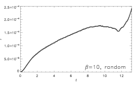
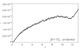
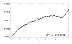
Figure 7: Light curves of the simulated slow jet (uniform background; closed boundary). The left column show the case with a random field orientation and $\beta=10$. The middle and right columns show cases with ordered local fields aligned with the matter flow velocities, with $\beta=10,1$ respectively. The integrated 6 cm synchrotron radio intensity $I$ light curves are on the top panels. Note that the fuzzy cocoon dominates the emission, masking variability on short timescales.

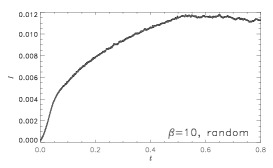
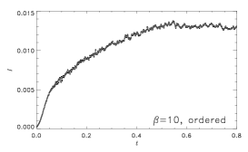
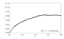
Figure 9: Same as Figure 7 but for the fast1 jet simulations. In the simulations, a fast jet propagates in uniform background medium, and a closed boundary condition is adopted. Compared to fast1o, there is more emission from the cocoon. The lightcurves thus track the expansion and emission fluctuations of the cocoon rather than the variability in the jet shocks.

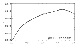
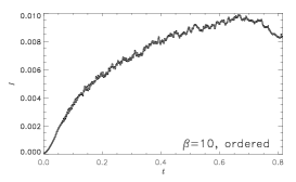
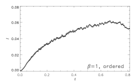
Figure 11: Same as Figure 7, but for the fast1rc jet simulations. In the simulations, a fast jet propagates in a uniform background medium, and a closed boundary condition is adopted. The jet plasma is relativistic, with $\gamma=4/3$.

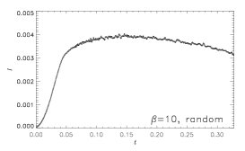
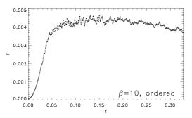
Figure 13: Synchrotron radio lightcurves of the fast2 jets, as in Figure 12. The simulations adopt same conditions as those in the fast2o jet simulations, except that the left boundary is reflective.

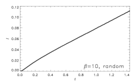
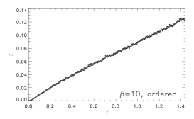
Figure 14: Synchrotron radio lightcurves (at 6 cm) of the fast3 jets. In the simulations, a fast jet propagates in a medium with a rising density. The jet generates an opaque fireball with no identifiable hotspot.

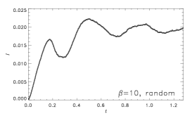
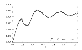
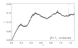
Figure 15: Synchrotron radio lightcurves of the fast4 jets, which penetrate a background density with ripply density variations.

In some simulations, large eddies with high concentrations of jet plasma are spun into large rings (by axisymmetry). Projections of these structures gives rise to patches with intense emission. The similarity of the light-curves in the “random” and “ordered” cases of Figures 7–15 demonstrates that these twinkles cause only local fluctuations. Their effects on spatially integrated intensity and Stokes parameters are usually negligible.

For synchrotron emission from relativistic electrons with a power-law energy distribution of an index $p$ gyrating in an orderly oriented magnetic field, the intensity spectral index $\alpha$ and the linear polarization $\Pi_{\rm L}$ are given by $\alpha=(p-1)/2$ and $\Pi_{\rm L}=(p+1)/(p+{\frac{7}{3}})$ respectively. Assuming $p=2.2$ in the calculations gives an index $\alpha=0.6$ of the synchrotron spectra and a maximum linear polarization $\Pi_{\rm L}\la 0.7$. The peak local values of $\Pi_{\rm L}$ in the simulated jets generally approach the theoretical maximum value of 0.7 regardless of the assigned magnetic-field configurations, as expected. Synchrotron emission has little intrinsic circular polarization (Legg & Westfold, 1968). However in a plasma, some circular polarization can be produced by Faraday conversion of the linear polarization components of radiation. (We discuss an aspect of polarization evolution briefly in §3.4, and in more detail in a forthcoming paper.)

Jet pinch shocks show a simple luminous knot where the biconical shock occurs. Hot-spots are composed of more complex and transient shocks, resulting in variable, closely spaced luminous patches. Resembling FR1 radio galaxies, the slow jets do not have a clear hotspot, and so the cocoon dominates the radio emission. For random fields, the jet is inconspicuous. There is little cocoon obscuration in the fast1o jets, and the jet shocks and the hotspot are distinct, like the morphology of FR2 sources.

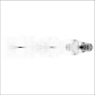
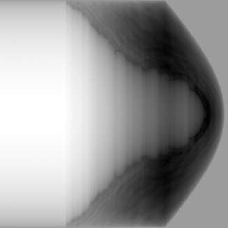
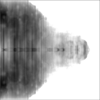
Figure 2: Emission images of the fast1o jet (top row) and the slow jet (bottom) at their late evolutionary stage. The image sizes are $150~{}{\rm kpc}\times 150~{}{\rm kpc}$. In both cases, $\beta=10$ and the field is quasi-poloidal ($\boldsymbol{B}\parallel\boldsymbol{v}$). Columns from left to right show: thermal bremsstrahlung X-rays, and synchrotron radio intensity ($I$). The emissions are linearly scaled. The synchrotron intensity is evaluated at 6 cm. The jet morphology in the non-thermal synchrotron X-ray images (unshown) is similar to that in the synchrotron radio emission image.

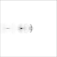
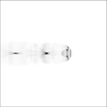
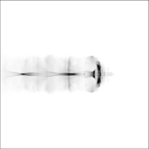
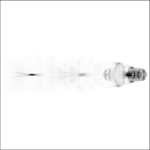
Figure 3: A time sequence of synchrotron radio intensity images of the fast1o jet at various evolutionary stages (frames 54, 108, 161, 215, 269, 323, 376 and 430, corresponding to times $t\approx 0.217,0.433,0.646,0.863,1.08,1.30,1.51,1.73$ Myr after the initial launch of the jet). In this calculation, $\beta=10$ and the field is ordered (quasi-poloidally $\boldsymbol{B}\parallel\boldsymbol{v}$).

3.1.2 alternative environments

We now comment on the characteristics of several variants of simulated fast jets:

fast1: The jets propagate in a uniform background density, as was the case for the fast1o jets. However a closed left boundary is now imposed. For fast1 jets, the jet itself and the shocks are generally distinguishable, but cocoon emission is more apparent. Many pinch shocks appear in the jet at the late stages of the evolution. The hotspot surges irregularly back and forth, typically traversing about a third the jet’s length.

fast1ro: The background is uniform and the left boundary is open to outflow, but the adiabatic index $\gamma=4/3$. Compared to fast1o, the cocoon is narrower and the jet takes longer to cross the grid.

fast1r: This is equivalent to fast1ro except that the left boundary is closed. Closure causes a wider cocoon to accumulate (as in fast1), despite the choice of $\gamma=4/3$.

fast2: The jets propagate in a radially declining background density. The jet emission remains distinctly visible through a cloudy cocoon (e.g. Figure 4). There are fewer pinch shocks than the case with a uniform background density, and the shocks are farther apart. The first two pinch shocks tend to outshine the hotspot. The hotspot throws off rings or filaments, as in the case with a uniform background density.

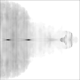
Figure 4: The last frame of the fast2 jet simulation. In the simulation, $\beta=10$, and the local magnetic field orientation is aligned with the flow velocity. Note that the hotspot is developing into a funnel morphology.

fast2o: An open boundary reduces the emission intensity of the cocoon. Apart from the reduction of the emission of the cocoon, the emission structure of the fast2o jets resembles that of the fast2 jets. The jet and hotspot are clearer than those of the fast2 jets.

fast3: A rising background density confines the expansion of the turbulent cocoon. The jet’s advance and cocoon’s growth decelerate (the front of the bow shock $x_{\rm s}\propto t^{0.44}$). We stop the simulation before the jet traverses the grid. With ordered fields and $\beta=10$, the late-time images only show a translucent cocoon with eddy induced substructures. (The case with $\beta=1$ is unassessable, because the twinkle artefacts dominate.) The jet is obscured and there is no apparent hotspot (see Figure 5).

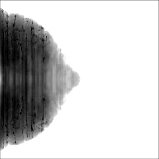
Figure 5: The 6 cm synchrotron radio intensity ($I$) map of the final frame of the fast3 jet simulation. In this simulation, the jet encounters a rising density profile. The magnetic field is quasi-poloidal ($\boldsymbol{B}\parallel\boldsymbol{v}$) and $\beta=10$.

fast4: The background medium has a ripply density variation. Naturally, the intensity of the jet emission varies as the jet propagates into these shells. In spite of the density variation, the jet morphologies are similar to those of the fast1 jets. The emission of the cocoon dominates in the intensity image, as in all cases with a closed left boundary. There is some subtle pinching of the cocoon outline where the jet reaches breakthrough points. At later evolutionary epochs, the jet head surges stochastically as far as half the jet’s length.

3.1.3 magnetic field configuration

In our standard calculations, we have assumed that the magnetic field is parallel to the flow, i.e.  $\boldsymbol{B}\parallel\boldsymbol{v}$. The field strength is parametrized, and its energy density scales with plasma thermal pressure. This corresponds to a quasi-poloidal field in the jet, but with “live” deviations at transient features such as shocks and vortices. As radio synchrotron radiation is determined by the magnetic field, we therefore investigate the jet emission for other magnetic field configurations. As a test of generality, we perform additional calculations with two alternative field configurations. (Figure 6).

In the sequence of the turn1 simulations, we rerun calculations for the fast1o simulations, with magnetic field directions perpendicular to local velocities. The cylindrical components are $\boldsymbol{B}=(B_{z},B_{r},B_{\varphi})\parallel(v_{r},-v_{z},0)$. Fields in the jet tend converge towards the axis (a quasi-radial configuration) which may be less physical than the usual $\boldsymbol{B}$ recipe. The emission morphology is essentially the same as that of the fast1o jets (top panels, Figure 6), but with a dark midline due to symmetry in $\boldsymbol{B}$.

In a futher sequence of the curl1 simulations, we set $\boldsymbol{B}\parallel\nabla\times\boldsymbol{v}$. This prescription guarantees $\nabla\cdot\boldsymbol{B}=0$, and yields quasi-toroidal fields around the jet. In the intensity images, the brightness is concentrated closer to the axis, but knots and the hotspot still appear in the usual places (bottom panels, Figure 6).

The general appearance of the jet and local features do not vary significantly under drastic changes of the $\boldsymbol{B}$ configuration. The 6 cm radio emission morphologies are limited by the underlying plasma density and pressure distributions. Within the luminous features, there are cosmetic variations caused by the minor polarisation effects and magnetic configuration. Mindful of these small differences, we proceed under the fiducial, quasi-poloidal assumption, and calculate radio maps and light-curves of fast jets penetrating various non-uniform media.

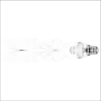
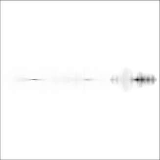
Figure 6: Synchrotron radio intensity ($I$) maps (at 6 cm) of the fast jet as in Figure 2 (fast1o), but with a different prescription for the magnetic field geometry. Top panel shows turn1, with a quasi-radial field ($\boldsymbol{B}\perp\boldsymbol{v}$). Bottom panel shows the result of a quasi-toroidal recipe (curl1, where $\boldsymbol{B}\parallel\nabla\times\boldsymbol{v}$).

3.2 Effects on jet evolution and emission variability

Figure 7 shows the evolution of the integrated intensity $I$, of the slow jet. Figures 8–15 are equivalent light-curves for the fast jets. In simulations where the hotspot is unambiguous and unobscured by the cocoon, we also present a local light-curve of the hotspot ($I_{\rm hs}(t)$). Here we define the instantaneous “hotspot” as the intensity maximum that is farthest right along the jet axis, and we integrate the emission within a projected radius of 20 pixels.

3.2.1 left boundary conditions

We have considered two types of left boundary conditions in the simulations. The open boundary condition mimics situations where the jets have drilled far from the central engine. This is appropriate for modeling the jets in giant radio galaxies. The closed boundary takes account of the effects of backflows and material accumulation. This is appropriate for modeling compact jets that are yet to break away from the core region, where backflows from both jet and counter-jet can interact with each other. Comparison of runs that differ at the left boundary (i.e. fast1o vs fast1 and fast2o vs fast2) shows that the (spatially integrated) temporal fluctuations are more rapid and have larger amplitudes for an open left boundary. This may be attributed to fact that the exit of plasma through the boundary leaves the unsteady structures (such as the jet shocks and hotspot) brighter than the cocoon. Also, with an open boundary condition, the cocoon contributes less to the total emission.

The cloudy cocoons of the $\gamma=5/3$ and $\gamma=4/3$ cases with closed boundaries have similar light curves (see Figures 9 and 11). The time taken to traverse the grid is not significantly affected by the alternative $\gamma$. The intensity reaches marginally higher levels for $\gamma=5/3$. When the left boundary is open (Figures 8 and 10) the effect of $\gamma$ is more conspicuous: $\gamma=4/3$ gives greater variability in the total intensity $I(t)$, as well as in bright features like the hotspot $I_{\rm hs}(t)$.

3.2.2 magnetic field structure

The differences in the intensity light curves between a random or an ordered field directions are more obvious for jets with a closed boundary and conspicuous cocoon (e.g. comparing $\beta=10$ columns within Figures 9, 13, 14 and 15). Integrated intensity and polarization profiles tend to be smoother in the random case, due to summation over incoherent zones of the image. Ordered fields following the velocity structure produce larger coherent emssion patches that evolve on the same temporal and spatial scales as the principal shocks and eddies. The hydrodynamic vacillation and surging of these structures is responsible for the high frequency quasi-periodicity apparent in the $I(t)$ curves.

3.2.3 approximate homology of intensities

A comparison of intensity light-curves calculated from the same simulation but with different $\beta$ shows that they are similar to within a scale factor of $\approx 0.16$ for each factor of $10$ increase in $\beta$. For cases with a closed boundary and a translucent cocoon (slow, fast1, fast2, fast3, fast4, fast1r) the homology holds at nearly all times. For the cases with an open left boundary and prominent jet shocks, the homology holds at late times (say when the front of the bow shock is beyond $x_{\rm s}>30~{}{\rm kpc}$) but the initial behaviours differ in detail. The scaling also breaks down temporarily around particularly bright and opaque features during the undulations of fast4b and flashes of the jet in fast1ro. The extreme choice of $\beta=1$ (strong field) makes more substructures opaque, and the scaling fails more often for higher $\beta$.

3.3 Jet variability and astrophysical implications

3.3.1 coruscating substructures

Evolution of local substructures along the midline of the image is shown by intensity slices in Figure 16. The hotspot has rapid structural and morphological variabilities: it throbs; it casts off vortex rings; it breaks and reforms. Identification of the hotspot is not always unambiguous. In one case (fast3), the hotspot and jet internal shocks are hidden within an opaque fireball. In general, the jet shocks have comparable intensities for cases with an open left boundary. However, when when left boundary is closed (fast1, fast2, fast4) the most persistently bright feature is the first jet shock. It outshines the jet hotspot, and would appear as a “pseudocore” as in jet observations (Jones, 1988; D’Arcangelo et al., 2007). At later evolutionary stages, a second pinching shock appears. It could be as bright as the hotspot, and it tends to migrate forwards (whereas the first shock hovers about a certain place).

Subtler diagonal streaks through the diagram represent more ephemeral shocks traversing the jet. The formation of bright emission knots in jets is sensitive to the environment, and the distribution of bright knots in the jets during any particular epoch could be a diagnostic of the density structure of the external medium. Our simulations have shown that the knots occur at nearly equal intervals for a uniform background (e.g. fast1, fast1o). The knots can also appear evenly spaced, for jets propagating through a medium with density that undulates about a mean (fast4). For a medium with a radially declining density (fast2o), the knots are closer together in the outskirts, beyond a long gap in the denser inner region.

3.3.2 intensity and jet advance

As shown by each wedge’s outline in Figure 16, the radio-emitting region advances as time elapses, and the front of the bow shock (denoted as $x_{\rm s}$, not illustrated) evolves similarly. Their evolutions are dependent on the external density profile. In a uniform medium, the jet advances and the cocoon expands with a gentle deceleration. The deceleration is more severe for media with a radially rising density (fast3). However, acceleration would occur if the density of the ambient medium decreases radially (fast2, fast2o).

In nature, the age of a jet activity episode is not directly observable, and neither are the density profiles of the medium in the vicinity (say, within a few tens kpc) of an AGN core. In contrast, the size of the system and the radio luminosities can be estimated from observational data. Thus, deriving a relation between the system size and radio luminosity from our simulations of time-dependent jets in various environments will provide a tool to constrain the age of jet activity episodes, and infer the ambient structure.

For models with an open left boundary, the light-curves are dominated by stochastic flashes from jet shocks. Once such a jet has grown long enough to have at least one pinch shock, there isn’t any tight relation between size and luminosity. (For fast1o, fast2o and fast1ro the light-curve at late times brightens and dims significantly on diverse timescales.) However for the models with a closed boundary (forming a foggy cocoon/lobe) relatively simple power-law relations occur.

The integrated intensity light curves $I(t)$ of the fast1 and fast2 jets are quite similar except that the latter drops at later times, when the jet encounters a significant density drop. During the initial rising stage of fast1 ($6.9~{}{\rm kpc}<x_{\rm s}<15~{}{\rm kpc}$) the total intensity grows like the plasma volume $I\propto x_{\rm s}^{3.02}\propto t^{3.82}$. The instantaneous peak intensity varies rapidly within a broad envelope that tends to run like $I_{\rm max}\propto x_{\rm s}^{0.78}\propto t^{-0.22}$. The growth curve steepens over time: $x_{\rm s}\propto t^{0.36}$ early on ($9~{}{\rm kpc}<x_{\rm s}<15~{}{\rm kpc}$). At later times ($19.5~{}{\rm kpc}<x_{\rm s}<120~{}{\rm kpc}$) the growth is $x_{\rm s}\propto t^{0.72}$, while the luminosity $I\propto x_{\rm s}^{0.61}\propto t^{0.44}$ and the peak $I_{\rm max}\propto x_{\rm s}^{-0.58}\propto t^{-0.42}$.

For fast2, the $x_{\rm s}=x_{\rm s}(t)$ curve steepens as the jet advances, but the index is $>1$ for most of the simulation. When $x_{\rm s}>30~{}{\rm kpc}$ the mean log-slope is $1.25$; when $x_{\rm s}>75~{}{\rm kpc}$ this rises to $1.53$. During the initial rise ($x_{\rm s}\la 12~{}{\rm kpc}$) the luminosity evolves as $I\propto x_{\rm s}^{3.02}\propto t^{2.45}$ and the peak $I_{\rm max}\propto x_{\rm s}^{0.69}\propto t^{0.33}$. After $x_{\rm s}\ga 12~{}{\rm kpc}$, the total intensity curve is nearly flat; the instantaneous peak values drop roughly like $I_{\rm max}\propto x_{\rm s}^{-0.66}$.

The fast3 jet inflates a globular cocoon/fireball with plasma accumulating at a constant rate, but a decelerating radial expansion. At later stages ($x_{\rm s}\ga 27~{}{\rm kpc}$), the growth curve is $x_{\rm s}\propto t^{0.44}$. As the cocoon is opaque for $\beta=1,10$ or $100$, the luminosity rises with the surface area, $I\propto x^{2.09}\propto t^{0.92}$, (Figure 14). The (noisy) envelope around the peak intensities rises slower, $I_{\rm max}\propto x^{1.56}\propto t^{0.69}$.

The fast4 jets (Figure 15), propagating in a ripply background, have lightcurves similar to fast1, but with undulations, as the jet is retarded by overdense shells, and then surges faster through underdense shells.

The light curves of the slow jets resemble the fast1 and fast2 jets initially and fast4 jets in the later stage. Despite the slow jet’s low Mach number, it advances with a power-law behaviour resembling that of fast1: $x_{\rm s}\propto t^{0.77}$ at late stages. The intensity laws are steeper than for fast1, $I\propto x_{\rm s}^{0.77}$ and $I_{\rm max}\propto x_{\rm s}^{-0.79}$. During the early rise, $x_{\rm s}\propto t^{0.57}$, $I\propto x_{\rm s}^{2.26}\propto t^{1.28}$ and $I_{\rm max}\propto x_{\rm s}^{0.60}$.

3.3.3 hotspot variability

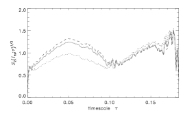
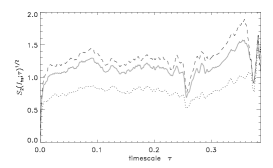
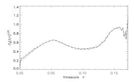
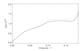
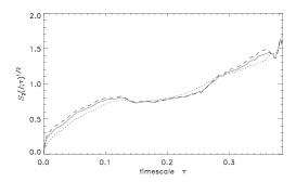
Figure 17: Structure functions of temporal variability in several quantities, for three open-boundary simulations (fast1o, fast2o and fast1ro). Here we take $\beta=10$ and the magnetic fields are quasi-poloidal ($\boldsymbol{B}\parallel\boldsymbol{v}$). The top row show structure functions of the hotspot intensity. The bottom row shows structure functions of the total intensity. Input variables to the structure functions are normalised to their respective means. Black-dotted, grey and black-dashed curves depict $\beta=1,10,100$ radiative transfer calculations respectively.

For models with an open boundary, the cocoon is mostly optically thin and the hotspot and other bright knots are relatively bare, so it is feasible to characterise their variabilities. In the top row of Figure 17 we plot the rms variability of the hotspot intensity, calculated from the temporal structure function of $I_{\rm hs}(t)$.

$$S_{2}(I_{\rm hs};\tau)={1\over{t_{\rm end}-\tau}}\int_{0}^{t_{\rm end}-\tau}\left[{I_{\rm hs}(t+\tau)-I_{\rm hs}(t)}\right]^{2}\ dt\ .$$ (7)

The bottom row shows corresponding structure functions calculated from the total integrated intensity, $I(t)$.

The basic jet in a uniform background (fast1o) has a structure function that rises towards longer timescales. Perhaps this reflects the trend for later flashes of the hotspots to be dimmer than earlier flashes (row two of Figure 8). The structure function is nonzero down to the smallest $\tau$ scales; implying that the time steps of our hydrodynamic snapshots are too coarse to resolve the vacillations of the brightest shocks. Changing the field geometry from random to ordered (e.g. with $\beta=10$ fixed) has no significant effect on the structure functions. Greater $\beta$ (weaker fields) raises the size of the $I_{\rm hs}$ fluctuations relative to the mean value, but the structure function retains the same shape in $\tau$.

With a declining density profile (fast2o) the structure function of $I_{\rm hs}$ reveals peaks around timescales $\tau\sim 0.05U_{t}$ and $0.16U_{t}$. The $0.05U_{t}$ bump may reflect the long interval between prolonged bright flares (seen in the initial episode and two later events in Figure 12). The peaks become sharper and more distinct for greater $\beta$: given the same flow evolution, a less magnetised hotspot flashes relatively more intensely. The structure function of total intensity $I(t)$ increases at longer timescales in the domain $\tau\la 0.10U_{t}$, perhaps describing with the brightenning trend, or the jump in $I$ around the time ($\approx 0.08U_{t}$) when the hotspot first separates from the pseudocore shock. The separation of subsequent diamond shocks at $\approx 0.02U_{t}$ intervals do not produce a clear feature in the structure function of $I$.

The jet with a flat background and relativistic equation of state (fast1ro) has a hotspot that fluctuates with similar power at all time scales. The structure function of $I_{\rm hs}(t)$ is similarly flat for $\beta=1,10$ and $100$. There is a slight hump at nearly the duration of the simulation; this may be due to the early, dim and steady phase at $t\la 0.9U_{t}$. The general flatness of the temporal structure functions suggests that the stochastic variation of the hotspot is like white noise (at least for the “hotspot” as we have presently defined it).

A radio galaxy of FR2 type has two opposite hotspots. Even if both the jet and the counter-jet are identical and unvarying at the nucleus, their hotspots vary independently: differently at any given epoch, but stochastically in essentially the same manner. We assume that the envelope or distribution of this innate variability is well characterised by the recorded variability during sufficiently late stages of the simulations. Frames occuring after the formation of the pseudocore shock should be an adequate selection.

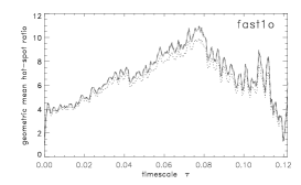
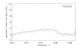
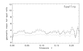
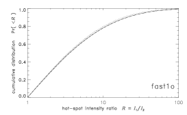
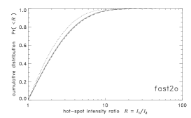
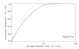
Figure 18: Illustration of the variability of the luminosity ratio of two hotspots in open-boundary simulations. (fast1o, fast2o and fast1ro from left to right respectively). The magnetic fields are quasi-poloidal, $\boldsymbol{B}\parallel\boldsymbol{v}$. The top row shows geometric mean hotspot ratios obtained from the structure function of $\ln(I_{\rm hs})$, for frames when the bow shock has advanced to $x_{\rm s}\geq 60~{}{\rm kpc}$. The bottom row shows cumulative distribution functions of the hotspot ratios at independent times. The dotted, grey and dashed curves depict cases with $\beta=1,10$ and $100$.

The upper panels of Figure 18 show what is effectively the goemetric mean of the hotspot ratios at a time separation $\tau$, as calculated from the structure function of the log-intensities, $\exp\sqrt{S_{2}(\ln(I_{\rm hs});\tau)}$. Typical values are $\approx 3$ for fast2o and fast1ro, but exceed ten at medium timescales for fast1o. In the lower panels of Figure 18 we draw random values of $I_{\rm hs}$ from times when $x_{\rm s}\geq 60~{}{\rm kpc}$, and plot the cumulative distribution function of the hotspot luminosity ratio. Our radiative transfer calculations imply that ratios of factors of a few can occur frequently by chance (even though the paired jets are equal and steady). Ratios in excess of ten are not rare for fast1o. For each simulation, the $\beta=1$ calculations give the least variable hotspot ratios. Perhaps this is because stronger magnetism raises the opacity of the brightest features, so that the foreground emitting surfaces effectively hide some of the variability farther from the virtual camera. The $\gamma=4/3$ simulation fast1ro shows this effect most strongly. The model with a radially declining density profile for the ambient medium (fast2o) shows less variable hotspot ratios than the standard uniform background (fast1o).

The general lesson to be drawn from these plots is that the apparent differences between opposite hotspots (during a single observational epoch) may be largely stochastic and transitory (even while the jet nozzles remain steady) and that caution is warranted when using these comparisons alone to constrain jet orientation, power or the behaviour of the nucleus. Doppler and orientation effects complicate matters further, calling for more arduous parameter surveys in future. To make precise observational inferrences, it may be best to involve complementary evidence from other bands, or to take a statistical view of large ensembles of AGN.

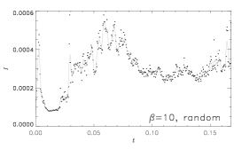
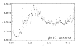
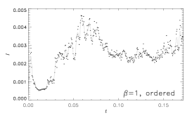
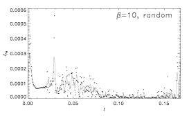
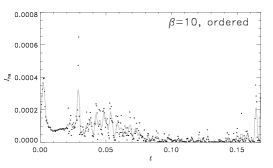
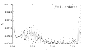
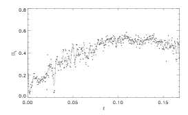
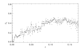
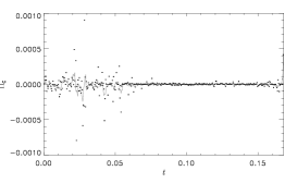
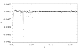
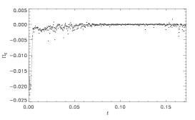
Figure 8: Intensity and polarization light-curves from radiative transfer calculations based on the fast1o jet simulations, where a fast jet propagates in a uniform background medium. An open left boundary is adopted. The jet emission is dominated by distinct and coherent features, such as the hotspot and jet shocks. Dots mark exact data; grey curves show a 5-point boxcar average. The spatially integrated intensity light curve (first row) is variable on many time scales. Hotspot intensity ($I_{\rm hs}$, within a 20-cell radius) light curves are in the second row. The hotspot is identified as the rightmost local maximum of intensity projected along the jet axis. The $I_{\rm hs}$ light curves fluctuate considerably more than those of the slow jet and the fast1 jet with closed boundary, as the hotspot of the fast1o jet is unobscured by the cocoon. The third and fourth rows show the integrated fractional linear and circular polarisation curves respectively.

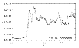
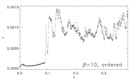
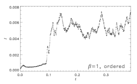
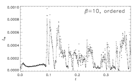
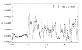
Figure 10: Same as Figure 7, but for the fast1ro jet simulations. In the simulations, a fast jet propagate in a uniform background medium, and an open boundary is adopted. The jet plasma is relativistic, with $\gamma=4/3$.

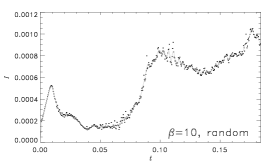
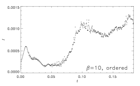
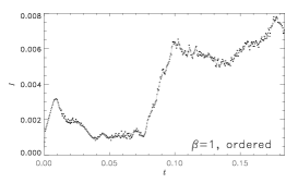
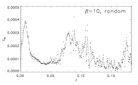
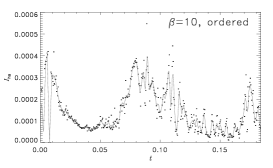
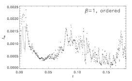
Figure 12: Synchrotron radio lightcurves (at 6 cm) of the fast2o jets. In the simulations, the jet traverses a background medium with a declining density. The left boundary is open. The magnetic field is random or ordered ($\boldsymbol{B}\parallel\boldsymbol{v}$) with $\beta$ values as indicated in each panel. The open left boundary reduces accumulation of the backflow, and he jet shocks outshine the cocoon emission, (cf.  the fast1o jet simulations). The fluctuations of the emission from the hotspot are visible in the $I_{\rm hs}$ lightcurves.

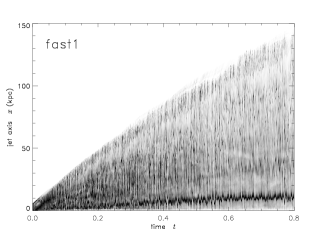
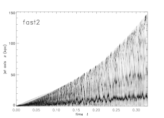
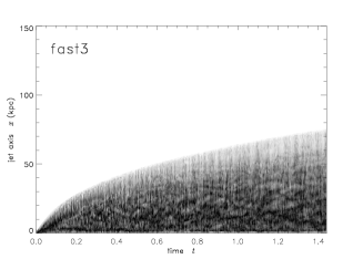
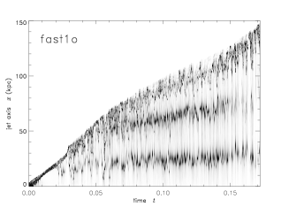
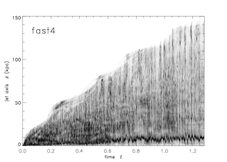
Figure 16: Evolution of intensity along the midline (projection of the jet axis) for the fast jet simulations (as annotated in respective panels, and assuming $\beta=10$). In cases with an open boundary condition (fast1o, fast2o) the jet shocks are brighter relative to the cocoon, and the hotspot is brighter relative to the pinch shocks. The density ripples in the background medium make little difference: fast4 resembles fast1. A radially declining density profile enables the jet’s advance to accelerate (fast2, fast2o) while a radially increasing profile restrains the expansion of a decelerating fireball (fast3). Except in fast3, the first jet shock is brightly visible, fluttering about its mean position. These figures are derived from Stokes maps made with ordered fields, and each vertical stripe is separately normalised.

3.4 stages of jet activity

Adiabatic hydrodynamic simulations are rescalable in the three physical units: length, time and density. The implementation of radiative transfer calculations, however, limits this freedom, because of the constraint that homologous models have the same optical depths (at corresponding scaled radiation frequencies) after rescaling the physical structure. Nonetheless, some freedom to rescale the models remains. Our models are therefore qualitatively relevant to analogous systems at smaller sizes, such as microquasar jets (although till this section we have interpreted our simulations with physical scales typical of large radio galaxies). For instance, a parsec-scale dwarf version of the confined fireball fast3 is conceivable.

The earliest stage of jet expansion involves a compact ball of jet plasma, with at most a single vortex cell (a much simpler backflow than at late times). A prominent termination shock shines brightly, but the jet is too short to fit any series of internal shocks. This is probably what occurs during flares by AGN and analogous microquasars (e.g. Fender et al., 2000, 2002; Macquart et al., 2002; Aller et al., 2003). As Figure 16 shows, for the fast jets with an open boundary the terminal shock dominates the luminosity during this stage ($t\la 0.02U_{t}$ for fast1o; $t\la 0.07U_{t}$ for fast2o). In corresponding models with a closed boundary (fast1; fast2) the fireball is more uniformly luminous due to the accumulated mass of plasma surrounding the sides of the jet.

The closed-boundary simulations represent jets still propagating near the nucleus. The accumulated plasma cocoon contributes a fuzz of radio emission on lateral scales a considerable fraction of the jet’s length. After the initial fireball stage, the locally brightest feature is usually the pseudo-core (first jet internal shock) but the extended fuzz contributes most of the integrated emission. In fast4 the ripply density background modulates the cocoon expansion dramatically (and causes a long-period throbbing in the $I(t)$ light curve), yet the position and variability of the pseudo-core are indistinguishable from the simpler fast1 case. In integrated intensity observations of closed systems, the fuzzy cocoon may wash out the intrinsic variability of the jet (as seen in the slowly varying $I(t)$ light curves). Spectral aging and dimming of the cocoon plasma (not included in our present simulations) would leave the jet relatively prominent at later times.

Simulations with an open left boundary represent jets that have penetrated far from the nucleus. Jet internal shocks and the hotspot then dominate the intensity maps at all times after the initial fireball. A comparison of fast1 with fast1o or fast2 with fast2o shows a greater separation between jet internal shocks in cases with an open boundary. When the background density profile decreases radially (fast2o) the pseudo-core is farther from the nucleus but the subsequent jet-shocks are closer together (compared to fast1o).

What about a jet injected into a pre-existing cavity, such as the ghost cocoon from a previous episode of nuclear activity? If the jet meets a smoothly rising density profile of the interstellar medium (like the case of fast3) a very different morphology emerges: a prolonged, highly opaque, frustrated fireball. This spheroid is edge-dim, unlike an early-stage fireball with bright termination shock. The frustrated fireball contains a more complex system of eddies, with dark creases visible at eddy interfaces nearer the surface. If these flows carry locally ordered magnetic fields, then these affect the radiative transfer differently to the simple fields in an “early fireball”. The “frustrated old fireball” and “early fireball” may have distinct polarization signatures. (We study these in detail in a forthcoming paper.)

As shown in Figure 16, although the internal jet shocks may hover about preferred points, they eventually drift upstream or downstream at apparently high velocities. Our integrated light profiles and hotspot light-curves for the open-boundary fast jets (upper two rows of Figures 8, 10 and 12) show that internal shocks and hotspots can brighten or fade by factors of a few on timescales of millennia or less. In smaller analogues of AGN, with shorter timescales, it is conceivable that an internal shock that fades, moves upstream and rebrightens might be mistaken for a new ejection there.

We noted that a pulse of circular polarization ($\Pi_{\rm C}$) can occur in the very initial stage of the simulations (bottom row of Figure 8), when the jet has a relatively coherent structure. The occurrence of a circular pulse is robust and seems insensitive to the density profile of the external medium. It occurs whether the magnetic configuration is set to be quasi-poloidal (dragged parallel to the jet flow) or quasi-toroidal (circulating around the flow), but not if the fields are randomly directed. Later, the circular polarisation is diluted rapidly as the jet evolves more numerous, complex, mutually incoherent emitting substructures. Thus, the circular polarization observed in AGN cores (e.g. Homan & Wardle, 1999; Rayner et al., 2000) probably indicates certain degrees of coherence in the emission region. Parametric models with turbulent or ordered, poloidal, toroidal or (intermediately) helical magnetic configurations have previously been applied to explain polarised emissions of AGN (e.g. Beckert & Falcke, 2002; Ruszkowski & Begelman, 2002; Enßlin, 2003; Gabuzda et al., 2008; Vitrishchak et al., 2008; Homan et al., 2009, and references therein). The essential ingredient in these models and in our time-dependent models is that magnetic fields vary along sightlines through the jet, so that linearly polarised radiation from distant locations undergoes Faraday conversion to circular modes in foreground plasma. As expected for this mechanism, we see that each spike in $|\Pi_{\rm C}|$ coincides with a dip in linear polarisation $|\Pi_{\rm L}|$ (e.g. third row, Figure 8). Circular polarization at a few percentage level was also seen in the initial stage of radio outburst in the microquasar GRO J1655$-$40 (Macquart et al., 2002). Our calculations for AGN jets show similar levels. A detailed discussion of time-dependent circular polarisation in microquasars is presented in Saxton et al. (2010) and a time-depedent polarimetry of AGN jets will be presented elsewhere (Saxton et al., in preparation).

4 CONCLUSIONS

We performed hydrodynamic simulations for jets encountering external media with conditions and density structures appropriate for active galaxies, and carried out time-dependent radiative transfer calculations to determine their polarization and emission properties. Our polarised radiative transfer formulation takes account of emission, absorption, re-emission, Faraday rotation and Faraday conversion. The radiative transfer equations were solved explicitly following the jet evolution. We applied this method to model the temporal evolution of emission from AGN jets interacting with a variety of structured ambient media. Our calculations showed that jet emissions vary considerably even though the launching conditions remain steady at the nucleus. Their variations are affected by the external density profile; thus environmental factors play an important role in determining the observed morphology and temporal properties of radio jets.

Our simulations show that the ambient media influence the distribution of jet knots and the relation between emission intensity and advance of the jet. Determining the jet knot distributions and the relation between intensity emission intensity and growth of jets can constrain the properties of the background gas. For instance, in an effectively closed cocoon (that contributes much of the radio luminosity) asymptotic power-laws appear to relate the elapsed time, jet length and total intensity. The indices of these relations depend on the density gradient of the ambient medium. For models with an open left boundary (with the jet terminus far from the nucleus) the radio intensity appears to flash independently of the jet length. The total intensity can fluctuate by factors of a few, and the hotspot can fluctuate by tens, within dynamically brief intervals (though longer than a human lifetime). Caution is needed when inferring the jet power from a single-epoch observations. In any particular epoch, the two hotspots may differ by three or more times in intrinsic brightness, even given identical and constant jet fluxes, and neglecting orientation and beaming effects.

Appendix A An remark on radiative transfer

In our calculations, radiative transfer is computed in eulerian cells that do not co-move with jet plasma. Thus, the transfer calculation has not included relative Doppler shift explicitly. We now assess whether or not the omission affects the calculated results significantly. The quantity $\nu^{-3}I_{\nu}$ is Lorentz invariant (where $\nu$ is the frequency and $I_{\nu}$ is the specific intensity). The radiative transfer equation in a co-moving frame thus takes the form:

$$\left[{\left(\frac{\nu}{\nu_{0}}\right)^{3}\hat{\mathbsf D}+\left(\frac{\nu}{\nu_{0}}\right)^{2}{\mathbsf K}}\right][[{\boldsymbol{I}}]]=\left(\frac{\nu}{\nu_{0}}\right)^{2}[[{\boldsymbol{J}}]]$$ (8)

(see e.g. Mihalas, 1970; Peraiah, 2002). Here, variables evaluated at the local rest frame are denoted by the subscript $0$. The co-moving transfer equation implies that Doppler effects are of the first order in $[1-({\boldsymbol{n}}\cdot{\boldsymbol{v}})/c]$ (see also Castor, 1972), where ${\boldsymbol{v}}$ is the medium local velocity. If ignoring terms of ${\cal O}[(v/c)^{2}]$ or higher and performing a series expansion, then the inclusion of Doppler shift simply modifies the propagation operator:

$$\partial_{s}\rightarrow\left({1-\frac{{\boldsymbol{n}}\cdot{\boldsymbol{v}}}{c}}\right)\partial_{s}+{\cal G}\ ,$$ (9)

where

$${\cal G}\approx 3\left\{{({\boldsymbol{n}}\cdot{\boldsymbol{\nabla}})\left({\frac{{\boldsymbol{n}}\cdot{\boldsymbol{v}}}{c}}\right)}\right\}\ .$$ (10)

The $[1-({\boldsymbol{n}}\cdot{\boldsymbol{v}})/c]$ term in front of the operator $\partial_{s}$ re-scales time and length along the ray and is unrelated to the absorption and re-emission of the radiation, and the Faraday effects on the Stokes parameters. The term ${\cal G}$, which is proportional to $\Delta\nu/\nu_{0}~{}(\equiv(\nu-\nu_{0})/\nu_{0})$, induces a “diffusive drift” of power across the frequency space. It can be omitted, provided that there is no sharp relativistic velocity gradient across the computational cells (e.g. in the presence of relativistic turbulence). Thus, omission of Doppler effects might distort the perceived time scale and length of the systems but would not affect the qualitative results obtained for the global morphology and polarization level of the jets. Simulations with explicit inclusion of Doppler effects require substantial modifications in the numerical algorithm and additional constraints set by the relativistic physics. We will leave this for a separate study.

References

- Aller et al. (2003) Aller H. D., Aller M. F., Plotkin R. M., 2003, Ap&SS, 288, 17
- Anderson et al. (1990) Anderson E., Bai Z., Bischof C., Demmel J., Dongarra J., Du Croz J., Greenbaum A., Hammarling S., McKenney A., Sorensen D., 1990, LAPACK, Technical Report 90-105. University of Tennessee, Knoxville, TN
- Barker et al. (2001) Barker V. A., Blackford L. S., Dongarra J., Du Croz J., Hammarling S., Marinova M., Waniewski J., Yalamov P., 2001, LAPACK95 Users’ Guide. SIAM
- Beckert & Falcke (2002) Beckert T., Falcke H., 2002, A&A, 388, 1106
- Begelman et al. (1984) Begelman M. C., Blandford R. D., Rees M. J., 1984, Reviews of Modern Physics, 56, 255
- Blondin & Lufkin (1993) Blondin J. M., Lufkin E. A., 1993, ApJS, 88, 589
- Carvalho & O’Dea (2002) Carvalho J. C., O’Dea C. P., 2002, ApJS, 141, 337
- Castor (1972) Castor J. I., 1972, ApJ, 178, 779
- Cavaliere & Fusco-Femiano (1976) Cavaliere A., Fusco-Femiano R., 1976, A&A, 49, 137
- Cenacchi et al. (2009) Cenacchi E., Kraus A., Beckert T., Mack K. ., 2009, A&A, accepted, arXiv:0901.4678
- Chakrabarti (1988) Chakrabarti S. K., 1988, MNRAS, 235, 33
- Cohn (1983) Cohn H., 1983, ApJ, 269, 500
- Colella & Woodward (1984) Colella P., Woodward P. R., 1984, Journal of Computational Physics, 54, 174
- D’Arcangelo et al. (2007) D’Arcangelo F. D., Marscher A. P., Jorstad S. G., Smith P. S., Larionov V. M., Hagen-Thorn V. A., Kopatskaya E. N., Williams G. G., Gear W. K., 2007, ApJ, 659, L107
- De Young (1986) De Young D. S., 1986, ApJ, 307, 62
- Enßlin (2003) Enßlin T. A., 2003, A&A, 401, 499
- Falle (1991) Falle S. A. E. G., 1991, MNRAS, 250, 581
- Falle et al. (1987) Falle S. A. E. G., Innes D. E., Wilson M. J., 1987, MNRAS, 225, 741
- Fender (2006) Fender R., 2006, in W. L., van der Klis. M., eds, Compact stellar X-ray sources Jets from X-ray binaries. Cambridge University Press, Cambridge, UK., pp 381–419
- Fender et al. (2000) Fender R., Rayner D., Norris R., Sault R. J., Pooley G., 2000, ApJ, 530, L29
- Fender et al. (2002) Fender R. P., Rayner D., McCormick D. G., Muxlow T. W. B., Pooley G. G., Sault R. J., Spencer R. E., 2002, MNRAS, 336, 39
- Gabuzda et al. (2008) Gabuzda D. C., Vitrishchak V. M., Mahmud M., O’Sullivan S. P., 2008, MNRAS, 384, 1003
- Hardee (1979) Hardee P. E., 1979, ApJ, 234, 47
- Hardee (1983) Hardee P. E., 1983, ApJ, 269, 94
- Hardee (1987) Hardee P. E., 1987, ApJ, 313, 607
- Hjellming & Johnston (1981) Hjellming R. M., Johnston K. J., 1981, Nature, 290, 100
- Hodge & Aller (1977) Hodge P. E., Aller H. D., 1977, ApJ, 211, 669
- Homan & Lister (2006) Homan D. C., Lister M. L., 2006, AJ, 131, 1262
- Homan et al. (2009) Homan D. C., Lister M. L., Aller H. D., Aller M. F., Wardle J. F. C., 2009, ApJ, accepted, arXiv:0902.0810
- Homan & Wardle (1999) Homan D. C., Wardle J. F. C., 1999, AJ, 118, 1942
- Homan & Wardle (2004) Homan D. C., Wardle J. F. C., 2004, ApJ, 602, L13
- Hughes et al. (1989a) Hughes P. A., Aller H. D., Aller M. F., 1989a, ApJ, 341, 54
- Hughes et al. (1989b) Hughes P. A., Aller H. D., Aller M. F., 1989b, ApJ, 341, 68
- Jones (1988) Jones T. W., 1988, ApJ, 332, 678
- Jones & O’Dell (1977) Jones T. W., O’Dell S. L., 1977, ApJ, 214, 522
- Koessl & Mueller (1988) Koessl D., Mueller E., 1988, A&A, 206, 204
- Komesaroff et al. (1984) Komesaroff M. M., Roberts J. A., Milne D. K., Rayner P. T., Cooke D. J., 1984, MNRAS, 208, 409
- Krause (2003) Krause M., 2003, A&A, 398, 113
- Krause (2005) Krause M., 2005, A&A, 431, 45
- Legg & Westfold (1968) Legg M. P. C., Westfold K. C., 1968, ApJ, 154, 499
- Macquart et al. (2002) Macquart J.-P., Wu K., Sault R. J., Hannikainen D. C., 2002, A&A, 396, 615
- Mantovani et al. (1997) Mantovani F., Junor W., Fanti R., Padrielli L., Saikia D. J., 1997, A&AS, 125, 573
- Marshall et al. (2002) Marshall H. L., Miller B. P., Davis D. S., Perlman E. S., Wise M., Canizares C. R., Harris D. E., 2002, ApJ, 564, 683
- McNamara et al. (2009) McNamara A. L., Kuncic Z., Wu K., 2009, MNRAS, 395, 1507
- Mihalas (1970) Mihalas D., 1970, Stellar atmospheres. Series of Books in Astronomy and Astrophysics, San Francisco: Freeman
- Mirabel & Rodríguez (1999) Mirabel I. F., Rodríguez L. F., 1999, ARA&A, 37, 409
- Norman et al. (1988) Norman M. L., Burns J. O., Sulkanen M. E., 1988, Nature, 335, 146
- Norman et al. (1982) Norman M. L., Winkler K.-H. A., Smarr L., Smith M. D., 1982, A&A, 113, 285
- O’Neill et al. (2005) O’Neill S. M., Tregillis I. L., Jones T. W., Ryu D., 2005, ApJ, 633, 717
- Peraiah (2002) Peraiah A., 2002, An Introduction to Radiative Transfer. Cambridge: University Press
- Perley et al. (1997) Perley R. A., Roser H.-J., Meisenheimer K., 1997, A&A, 328, 12
- Perlman & Wilson (2005) Perlman E. S., Wilson A. S., 2005, ApJ, 627, 140
- Rayner et al. (2000) Rayner D. P., Norris R. P., Sault R. J., 2000, MNRAS, 319, 484
- Roeser & Meisenheimer (1987) Roeser H.-J., Meisenheimer K., 1987, ApJ, 314, 70
- Rosen et al. (1999) Rosen A., Hughes P. A., Duncan G. C., Hardee P. E., 1999, ApJ, 516, 729
- Ruszkowski & Begelman (2002) Ruszkowski M., Begelman M. C., 2002, ApJ, 573, 485
- Saxton et al. (2002) Saxton C. J., Bicknell G. V., Sutherland R. S., 2002, ApJ, 579, 176
- Saxton et al. (2005) Saxton C. J., Bicknell G. V., Sutherland R. S., Midgley S., 2005, MNRAS, 359, 781
- Saxton et al. (2001) Saxton C. J., Sutherland R. S., Bicknell G. V., 2001, ApJ, 563, 103
- Saxton et al. (2002) Saxton C. J., Sutherland R. S., Bicknell G. V., Blanchet G. F., Wagner S. J., 2002, A&A, 393, 765
- Saxton et al. (2010) Saxton C. J., Wu K., Macquart J.-P., 2010, A&A, submitted
- Smith et al. (1985) Smith M. D., Norman M. L., Winkler K.-H. A., Smarr L., 1985, MNRAS, 214, 67
- Sokoloski et al. (2004) Sokoloski J. L., Kenyon S. J., Brocksopp C., Kaiser C. R., Kellogg E. M., 2004, in Tovmassian G., Sion E., eds, Revista Mexicana de Astronomia y Astrofisica Conference Series Vol. 20 of Revista Mexicana de Astronomia y Astrofisica Conference Series, Jets from Accreting White Dwarfs. pp 35–36
- Sutherland et al. (2003) Sutherland R. S., Bisset D. K., Bicknell G. V., 2003, ApJS, 147, 187
- Taylor et al. (1986) Taylor A. R., Seaquist E. R., Mattei J. A., 1986, Nature, 319, 38
- Tingay et al. (2008) Tingay S. J., Lenc E., Brunetti G., Bondi M., 2008, AJ, 136, 2473
- Vitrishchak et al. (2008) Vitrishchak V. M., Gabuzda D. C., Algaba J. C., Rastorgueva E. A., O’Sullivan S. P., O’Dowd A., 2008, MNRAS, 391, 124
- Wegg (2003) Wegg C., 2003, MSci thesis, University College London
- Weiler & de Pater (1983) Weiler K. W., de Pater I., 1983, ApJS, 52, 293
- Wilson et al. (2001) Wilson A. S., Young A. J., Shopbell P. L., 2001, ApJ, 547, 740