Continuous time Ehrenfest process in term structure modelling

Abstract

In this paper, a finite-state mean-reverting model for the short-rate, based on the continuous time Ehrenfest process, will be examined. Two explicit pricing formulae for zero-coupon bonds will be derived in the general and the special symmetric cases. Its limiting relationship to the Vasicek model will be examined with some numerical results.

Keywords: ehrenfest model, interest rate derivatives, short-rate, term structure, vasicek model, zero-coupon bond

Classification: Primary 91G30
Classification: Secondary 60J28; 91G20; 33C52

1 Introduction

One of the fundamental approaches to term structure modelling is based on the specification of the short-term interest rate – the short-rate. Vasicek [20] first introduced a mean-reverting short-rate model with Gaussian distribution and derived a closed-form representation for the zero-coupon bond (ZCB) price. Since then, a variety of short-rate models have become established, each having its advantages and disadvantages.

Albeit the earliest, Vasicek’s model is still very popular among practitioners owing to its analytical tractability with regard to ZCB prices and European options thereof. Unfortunately, the model has some shortcomings. The most prominent of these is the possibility for the interest rates to become negative – a fact relating to all models with Gaussian distribution. Even though the probability of negative rates is rather small, not only is the realism of the model questionable, but also problems may appear while valuing ZCBs with a long time to maturity and a low interest rate level.

The idea of using both the discrete and the continuous time versions of the Ehrenfest process in finance is well-known. The discrete time approach was used, for example , by Okunev and Tippett [14] in modelling accumulated cashflows, by Takahashi [19] in exploring changes in stock prices and exchange rates for currencies, and by Buehlmann [5] in modelling interest rates. With regard to the modelling of interest rates, it seems that the discrete time approach leads in general only to a recursively computable term structure. Sumita, Gotoh and Jin [17] studied the passage times and the historical maximum of the Ornstein-Uhlenbeck process via an approximation by means of a special case of the continuous time Ehrenfest process.

This paper proposes a finite-state mean-reverting model for the short-rate related to the continuous time Ehrenfest process. By choosing arbitrary lower and upper bounds for the rate, the respective short-rate process can be seen as a suitably linearly transformed birth-and-death process on $\{0,1,\dots,N\},\ N\in\mathbb{N}$. By choosing the lower bound as non-negative, the problem of negative interest rates can be avoided. Furthermore, the model allows an explicit evaluation of ZCB prices. In this way, the model aims at realism and analytical tractability.

The main outcome of the paper is the derivation of pricing formulae for ZCBs in the general and the special symmetric cases of the model. In both cases the arbitrage-free ZCB price at time $t$ and maturity $T$ is given as follows:

$$P(t,T)=C\cdot P_{1}(t,T)^{k}\cdot P_{0}(t,T)^{N-k},$$

where $C$ is a constant, $k\in\{0,1,\dots N\},$ and $P_{1}$ and $P_{0}$ can be expressed in terms of the $\ {}_{1}F_{1}$ hypergeometric functions of a matrix argument given in Section 2 (see also [7]). In the general case the model is governed by five parameters – a valuable fact considering the fitting of the model to the market data. The special case provides four parameters and is characterized by the symmetry of the underlying distribution with respect to the mean-reverting value. The advantage here is that we have more tractable expressions of $P_{1}$ and $P_{0}$ from the computational point of view. Moreover, a suitably transformed symmetric case of the model yields the Vasicek model in the limit as $N$ tends to infinity.

The paper is organized as follows: the following section gives a short review of the special functions we shall encounter throughout this paper. Section three deals with the Ehrenfest process in continuous time. The main results are given in section four, where the Ehrenfest short-rate model is defined and the ZCB pricing formulae are derived. The fifth section gives an overview of the Vasicek model and its limiting relationship to the Ehrenfest short-rate model. Section six illustrates the advantages of the Ehrenfest short-rate model.

This paper comprises part of my Ph.D. project at the Technische Universität Dortmund. I am deeply indebted to Professor Michael Voit for his patience and for being a wonderful research mentor.

2 Special functions and orthogonal polynomials

Throughout this paper we will make use of some well-known facts concerning the Krawtchouk polynomials (see [10], [18] and [21]) and $\ {}_{1}F_{1}$ functions (see [7]), as well as some of their practical implications. In the interests of clarity we give in this section an overview of these special functions.

Hypergeometric functions of matrix argument

2.1 Definition.

1. A partition $m:=(m_{1},m_{2},\dots,m_{n})$ is an $n$-tuple $(n\in\mathbb{N})$ of non-negative integers such that $m_{1}\geq m_{2}\geq\dots\geq m_{n}.$

2. For a partition $m$ the generalized Pochhammer symbol is defined by

   $$[a]_{m}:=\prod_{j=1}^{n}(a-j+1)_{m_{j}},$$

   where $(a)_{k}:=a(a+1)\cdots(a+k-1)$ denotes the usual Pochhammer symbol.

3. For a partition $m$ the normalized Schur function of index $m$ is defined by

   $$Z_{m}(z):=|m|!\cdot\frac{\prod_{1\leq j<k\leq n}(m_{j}-m_{k}-j+k)}{\prod_{j=1}^{n}(m_{j}+n-j)!}\cdot\frac{\det\bigl{(}z_{i}^{m_{j}+n-j}\bigr{)}}{\prod_{1\leq i<j\leq n}(z_{i}-z_{j})}.$$

4. The hypergeometric function ${}_{p}F_{q}$ of matrix argument is defined as a real-analytic function on the space $S_{n}\ (n\in\mathbb{N})$ of $n\times n$ Hermitian matrices with eigenvalues $z:=(z_{1},\dots,z_{n})^{T}\in\mathbb{R}^{n},$ and is given by the series

   $$_{p}F_{q}(a_{1},\dots,a_{p};b_{1},\dots,b_{q};z):=\sum_{j=0}^{\infty}\frac{1}{j!}\sum_{|m|=j}\frac{[a_{1}]_{m}\dots[a_{p}]_{m}}{[b_{1}]_{m}\dots[b_{q}]_{m}}\cdot Z_{m}(z),$$ (1)

   where, for $1\leq i\leq p$ and $1\leq j\leq q,\ a_{i}\in\mathbb{C}$ and none of the numbers $-b_{i}+j-1$ is a non-negative integer.

We will be particularly concerned with the ${}_{1}F_{1}$ function, which is also known as the confluent hypergeometric function of matrix argument. From Theorem 4.1 in [7] we know that it converges absolutely for all $z\in S_{n}.$ An important result, that will be crucial later on, is given without proof in the following remark (see [7], p. 25).

2.2 Remark.

Let $\Delta_{n}$ denote the standard simplex in $\mathbb{R}^{n}\ (n\in\mathbb{N}),$ defined by

$$\Delta_{n}:=\left\{(x_{1},\dots,x_{n})\in\mathbb{R}^{n}:x_{i}\geq 0,i=1,\dots n,\sum_{i=1}^{n}x_{i}\leq 1\right\}.$$ (2)

Then for $a>0$ the following equation holds:

$$_{1}F_{1}(1;a+n;z)=(a)_{n}\int_{\Delta_{n}}\left(1-\sum_{i=1}^{n}\right)^{a-1}\cdot\exp\left(\sum_{i=1}^{n}z_{i}x_{i}\right)\,dx_{1}\dots dx_{n}.$$ (3)

In order to compute the ${}_{p}F_{q}$ function numerically we truncate the series (1) by $m\leq H$ as follows:

$$_{p}F_{q}^{H}(a_{1},\dots,a_{p};b_{1},\dots,b_{q};z):=\sum_{j=0}^{H}\frac{1}{j!}\sum_{|m|=j}\frac{[a_{1}]_{m}\dots[a_{p}]_{m}}{[b_{1}]_{m}\dots[b_{q}]_{m}}\cdot Z_{m}(z).$$ (4)

Koev and Edelman [11] provide an effective algorithm for computing the ${}_{p}F_{q}^{H}$ function. For $z\in S_{n}$ the complexity of their algorithm is linear in $n$ and subexponential in $H,$ which is acceptable if we consider the fast convergence of the power series (4).

Krawtchouk polynomials

For given $N\in\mathbb{N}$ and $0<p=1-q<1$ the Krawtchouk polynomials $K_{l}(x):=K_{l}(x;N;p)$ are the orthogonal polynomials that relate to the binomial distribution $B_{N,p}$ and the probability mass function $\omega(x):=\binom{N}{x}p^{x}q^{N-x}$ at the points $x=0,1,\dots,N.$ They can be defined in two different, but equivalent ways.

2.3 Definition.

For $x,l\in\{0,1,\dots,N\}$ we set

$$K_{l}(x):=\,_{2}\mathcal{F}_{1}(-l,-x;-N;1/p):=\sum_{k=0}^{N}\frac{(-l)_{k}(-x)_{k}}{(-N)_{k}k!}\left(\frac{1}{p}\right)^{k},$$ (5)

or

$$K_{l}(x):=\binom{N}{l}^{-1}\sum_{k=0}^{N}(-1)^{k}\binom{N-x}{l-k}\binom{x}{k}\left(\frac{q}{p}\right)^{k},$$ (6)

where $\,{}_{2}\mathcal{F}_{1}$ is the classical Gauss hypergeometric function (see [18], §4.21).

Definition 2.3 leads to the following basic well-known properties:

2.4 Lemma.

1. Symmetry:

   $$K_{l}(x)=K_{x}(l)$$ (7)

   for all $x,l\in\{0,1,\dots,N\}$.

2. $K_{0}(x)=K_{l}(0)=1$ for all $x,l\in\{0,1,\dots,N\}$.

3. $K_{1}(x)=1-\frac{x}{Np}.$

4. Generating function:

   $$\bigl{(}1-\frac{q}{p}\cdot s\bigr{)}^{i}\cdot\bigl{(}1+s\bigr{)}^{N-i}=\sum_{k=0}^{N}\binom{N}{l}K_{l}(i)s^{l}$$ (8)

   for all $x\in\{0,1,\dots,N\}.$

5. Recurrence relation:

   $$-xK_{l}(x)=(N-l)pK_{l+1}(x)-\left[(N-l)p+lq\right]K_{l}(x)+lqK_{l-1}(x)$$ (9)

   for all $x,l\in\{0,1,\dots,N\}.$

6. Orthogonality relation:

   $$\sum_{x=0}^{N}K_{l}(x)K_{m}(x)\omega(x)=\frac{\delta_{l,m}}{\pi_{l}},$$ (10)

   where

   $$\pi_{l}:=\binom{N}{l}\left(\frac{p}{q}\right)^{l}=\omega(l)q^{-N}$$ (11)

   for all $l,m\in\{0,1,\dots,N\}.$

7. For $l,m\in\{0,1,\dots,N\},\ m\leq l$

   $$B_{m,l}:=\sum_{x=0}^{N}xK_{l}(x)K_{m}(x)\omega(x)=\begin{cases}\phantom{-}0\quad&\text{if}\quad m\leq l-2,\\ -lq\pi_{l-1}\quad&\text{if}\quad m=l-1,\\ \phantom{-}((N-l)p+lq)\pi_{l}\quad&\text{if}\quad m=l.\end{cases}$$ (12)

   Note that $B_{l,m}=B_{m,l}.$

Proof.

$(a)-(e)$ follow from (5), $(f)$ follows from (6) and $(g)$ is a direct application of (9) and (10) (see e.g. [18], §2.82). ∎

3 Original Ehrenfest model

The original Ehrenfest model describes the heat exchange between two isolated bodies, each of arbitrary temperature. The temperatures are symbolized by the number of fluctuating balls in two urns with a total of $N\in\mathbb{N}$ balls. For details of the continuous and discrete time versions of the model we refer to [2], [10], [12] and [16].

In this section we shall discuss the continuous time Ehrenfest process. Primarily, its representation as a sum of independent simple processes will allow us to show the main result of this paper which comes up in the next section. Furthermore, we examine the transition semigroup of the Ehrenfest process and explore some of its basic properties.

Ehrenfest process

Let $N$ balls, initially distributed between urns I and II, fluctuate independently in continuous time between the two urns. We fix a fluctuation parameter $\lambda>0$ and independent Poisson processes $(N^{1}_{t})_{t\geq 0},\dots,(N^{N}_{t})_{t\geq 0}$ with intensity $\lambda.$ Let $(\hat{Y}_{n})_{n\in\mathbb{N}}$ be a Markov chain with the state space $\{0,1\}$ and transition probability matrix

$$P:=\begin{pmatrix}1-\alpha&\alpha\\ \beta&1-\beta\\ \end{pmatrix}.$$ (13)

Then, the subordinated Markov chain $(Y^{l}_{t}:=\hat{Y}_{N^{l}_{t}})_{t\geq 0}$ describes the state of the $l$-th ball at time $t,$ where $Y^{l}_{t}=1$ or $0$ when the $l$-th ball is in urn I or II respectively. Hence,

$$\Bigl{(}X_{t}:=\sum_{l=1}^{N}Y^{l}_{t}\Bigr{)}_{t\geq 0}$$ (14)

is a Markov process with the state space $E:=\{0,1,\dots,N\},$ denoting the number of balls in urn I at time $t.$ We call $(X_{t})_{t\geq 0}$ the (continuous time) Ehrenfest process. A discrete time version of (14) with arbitrary $\alpha$ and $\beta$ was studied by Kraft and Schaefer [12].

3.1 Remark.

1. A special case of (14) with $\alpha=\beta=1,$ first suggested by Siegert [16] and also studied by Bingham [2], where the transitions become “deterministic” in the sense of switching between the states 0 and 1, will be important for us later on in Section 4. (Its discrete time analogue leads to the original Ehrenfest chain).

2. Karlin and McGregor [10] provided an alternative but equivalent definition of (14) as a birth-and-death process with the state space $E$. Here, the time intervals between events are independently exponentially distributed with intensity $\gamma,$ and for $i\in E$ the birth and death rates are $\lambda_{i}:=\gamma\alpha\frac{(N-i)}{N}$ and $\mu_{i}=\gamma\beta\frac{i}{N}$ respectively, where $\alpha$ and $\beta$ are given as above. It can be verified that in the setting at hand $\gamma=\lambda N.$

Before computing the transition semigroup of $(X_{t})_{t\geq 0}$ we need the following result:

3.2 Lemma.

The transition semigroup of $(Y^{l}_{t})_{t\geq 0}$ is given by

$$P(t)=\begin{pmatrix}q+pe^{-\lambda(\alpha+\beta)t}\ &p-pe^{-\lambda(\alpha+\beta)t}\\ q-qe^{-\lambda(\alpha+\beta)t}\ &p+qe^{-\lambda(\alpha+\beta)t}\\ \end{pmatrix},$$ (15)

where $p:=\frac{\alpha}{\alpha+\beta}$ and $q:=1-p.$

Proof.

Since $(Y^{l}_{t})_{t\geq 0}$ is a Markov chain subordinated by a Poisson process with index $\lambda,$ the associated transition semigroup can be written as (see [3], p.333)

$$P(t)=e^{-\lambda t}\cdot e^{\lambda tP}:=e^{-\lambda t}\sum_{n=0}^{\infty}\frac{(\lambda t)^{n}}{n!}P^{n}.$$ (16)

We can avoid the computation of $P^{n}$ by writing $P=\mu S+(1-\mu)I,$ where $S=\begin{pmatrix}q\ &p\\ q\ &p\\ \end{pmatrix}$ is a stochastic matrix with $S^{2}=S,\ I$ is the identity matrix, and $\mu:=\alpha+\beta.$ Then, (16) becomes

$$P(t) = e^{-\lambda t}\cdot e^{\lambda t(\mu S+(1-\mu)I)}=e^{-\lambda t}\cdot e^{\lambda\mu tS}\cdot e^{\lambda(1-\mu)tI}$$

$$= e^{-\lambda\mu t}\cdot e^{\lambda\mu tS}=e^{-\lambda(\alpha+\beta)t}\sum_{n=0}^{\infty}\frac{(\lambda(\alpha+\beta)t)^{n}}{n!}S^{n}.$$

Since $S^{n}=S$ for all $n\in\mathbb{N},$ we can easily compute the above series, which completes the proof. ∎

3.3 Remark.

Analogue to the proof above, we see that a variation of $\alpha$ and $\beta$ in (15) can be equivalently described as a suitable modification of $p$ and $\lambda$. Thus, the distribution of $(Y_{t})_{t\geq 0}$ depends only on the two parameters $p$ and $\lambda$ or, equivalently, $\alpha$ and $\beta$.

3.4 Theorem.

(Properties of the Ehrenfest process) Let $(X_{t})_{t\geq 0}$ be the Ehrenfest process given by (14).

1. The transition probabilities $p_{ij}(t):=\mathbb{P}(X_{t+s}=j|X_{s}=i)$ are given by

   $$p_{ij}(t)=\binom{N}{j}\left(\frac{p}{q}\right)^{j}\sum_{x=0}^{N}\binom{N}{x}p^{x}q^{N-x}K_{i}(x)K_{j}(x)e^{-\lambda(\alpha+\beta)xt},$$ (17)

   where $p:=\frac{\alpha}{\alpha+\beta},\ q:=1-p,$ and $K_{i}(.):=K_{i}(.;p;N)\ (i\in E)$ are the Krawtchouk polynomials as given in Definition 2.3 .

2. The conditional mean and variance of $(X_{t})_{t\geq 0}$ are given by

   $$\mathbb{E}[X_{t}|X_{0}=i] = Np-(Np-i)e^{-\lambda(\alpha+\beta)t},$$ (18)

   $$\mathbb{V}ar[X_{t}|X_{0}=i] = Np(1-p)+(Np-i)(2p-1)e^{-\lambda(\alpha+\beta)t}$$

   $$-(Np-i)^{2}(2p-1)e^{-2\lambda(\alpha+\beta)t}.$$

3. The stationary distribution is the limiting distribution, and it is given by the binomial distribution $B_{N,p}$ on $E$ with parameter $p.$

Proof.

Ad $(a):$ The proof here is similar to that in [2]. First, we compute the moment-generating function of $(Y^{l}_{t})_{t\geq 0},$ given $Y^{l}_{0}.$ In the following we suppress the dependence of $(Y^{l}_{t})_{t\geq 0}$ on $l$ when it is clear from the context. From Lemma 3.2 we have

$$\mathbb{E}\left[z^{Y_{t}}\big{|}Y_{0}=1\right] = p_{10}(t)+p_{11}(t)z=q+pz-q(1-z)e^{-\lambda(\alpha+\beta)t},$$

$$\mathbb{E}\left[z^{Y_{t}}\big{|}Y_{0}=0\right] = p_{00}(t)+p_{01}(t)z=q+pz+p(1-z)e^{-\lambda(\alpha+\beta)t}.$$

Since $(Y^{l}_{t})_{t\geq 0}$ are independent for all $l=1,\dots,N,$ we obtain from (14) the moment-generating function of $(X_{t})_{t\geq 0},$ given $X_{0}=i,$ as follows:

$$\sum_{j=0}^{N}p_{ij}(t)z^{j} = \mathbb{E}\left[z^{\sum_{l=1}^{N}Y^{l}_{t}}\big{|}X_{0}=i\right]=\mathbb{E}\left[\prod_{l=1}^{N}z^{Y^{l}_{t}}\big{|}X_{0}=i\right]$$

$$= \mathbb{E}\left[z^{Y_{t}}\big{|}Y_{0}=1\right]^{i}\cdot\mathbb{E}\left[z^{Y_{t}}\big{|}Y_{0}=0\right]^{N-i}$$

$$= \left[q+pz-q(1-z)e^{-\lambda(\alpha+\beta)t}\right]^{i}\cdot\left[q+pz+p(1-z)e^{-\lambda(\alpha+\beta)t}\right]^{N-i}$$

$$= (q+pz)^{N}\cdot\left[1-\frac{q}{p}\cdot\frac{p(1-z)}{q+pz}e^{-\lambda(\alpha+\beta)t}\right]^{i}\cdot\left[1+\frac{p(1-z)}{q+pz}e^{-\lambda(\alpha+\beta)t}\right]^{N-i}.$$

Applying $(a)$ and $(d)$ of Lemma 2.4, we obtain

$$\sum_{j=0}^{N}p_{ij}(t)z^{j} = (q+pz)^{N}\sum_{x=0}^{N}\binom{N}{x}K_{i}(x)\left(\frac{p(1-z)}{q+pz}e^{-\lambda(\alpha+\beta)t}\right)^{x}$$

$$= \sum_{x=0}^{N}\binom{N}{x}K_{i}(x)(q+pz)^{N-x}p^{x}(1-z)^{x}e^{-\lambda(\alpha+\beta)xt}$$

$$= \sum_{x=0}^{N}\binom{N}{x}p^{x}q^{N-x}K_{i}(x)\left(1-\frac{q}{p}\cdot\frac{pz}{q}\right)^{x}\left(1+\frac{pz}{q}\right)^{N-x}e^{-\lambda(\alpha+\beta)xt}.$$

Applying (8) once again, we get

$$\sum_{j=0}^{N}p_{ij}(t)z^{j} = \sum_{x=0}^{N}\binom{N}{x}p^{x}q^{N-x}K_{i}(x)\left[\sum_{j=0}^{N}\binom{N}{j}K_{j}(x)\left(\frac{pz}{q}\right)^{j}\right]e^{-\lambda(\alpha+\beta)xt}$$

$$= \sum_{j=0}^{N}\left[\binom{N}{j}\left(\frac{p}{q}\right)^{j}\sum_{x=0}^{N}\binom{N}{x}p^{x}q^{N-x}K_{i}(k)K_{j}(x)e^{-\lambda(\alpha+\beta)xt}\right]z^{j}.$$

Equating coefficients of $z^{j}$ completes the proof of the claim.
Ad $(b):$ Combining (17) with results $(a),(b)$ and $(g)$ of Lemma 2.4, we obtain

$$\mathbb{E}[X_{t}|X_{0}=i] = \sum_{j=0}^{N}j\cdot p_{ij}(t)=\sum_{j=0}^{N}j\cdot\omega(j)\sum_{x=0}^{N}\pi_{x}K_{i}(x)K_{j}(x)e^{-\lambda(\alpha+\beta)xt}$$ (20)

$$= \sum_{x=0}^{N}\pi_{x}K_{i}(x)e^{-\lambda(\alpha+\beta)xt}\sum_{j=0}^{N}j\cdot K_{x}(j)\omega(j)$$

$$= \sum_{x=0}^{N}\pi_{x}B_{0,x}K_{i}(x)e^{-\lambda(\alpha+\beta)xt},$$

where $B_{0,x}\neq 0$ for $x\in\{0,1\}$ as given in (12), which implies (18). Moreover,

$$\mathbb{E}[X^{2}_{t}|X_{0}=i] = \sum_{j=0}^{N}j^{2}\cdot p_{ij}(t)=\sum_{j=0}^{N}j^{2}\cdot\omega(j)\sum_{x=0}^{N}\pi_{x}K_{i}(x)K_{j}(x)e^{-\lambda(\alpha+\beta)xt}$$

$$= \sum_{x=0}^{N}\pi_{x}K_{i}(x)e^{-\lambda(\alpha+\beta)xt}\sum_{j=0}^{N}j^{2}\cdot K_{x}(j)\omega(j)$$

$$= \sum_{x=0}^{N}\pi_{x}K_{i}(x)e^{-\lambda(\alpha+\beta)xt}\sum_{j=0}^{N}j\cdot\omega(j)\Bigl{[}-(N-x)pK_{x+1}(j)$$

$$\qquad\qquad\qquad\quad\ +\left[(N-x)p+xq\right]K_{x}(j)-xqK_{x-1}(j)\Bigr{]}$$

$$= \sum_{x=0}^{N}\pi_{x}K_{i}(x)e^{-\lambda(\alpha+\beta)xt}\Bigl{[}-(N-x)pB_{0,x+1}$$

$$\qquad\qquad\qquad\qquad\ \ +\left[(N-x)p+xq\right]B_{0,x}-xqB_{0,x-1}\Bigr{]},$$

where $B_{0,x}$ is given by (12). A straightforward computation of

$$\mathbb{V}ar[X_{t}|X_{0}=i]=\mathbb{E}[X^{2}_{t}|X_{0}=i]-\mathbb{E}[X_{t}|X_{0}=i]^{2}$$

leads immediately to ($(b)$).
Ad $(c):$ Clear. ∎

4 Ehrenfest short-rate model

In this section we introduce a finite-state mean-reverting short-rate model associated with the continuous time Ehrenfest process (14) and give its basic properties. As a main result, we exploit the algebraic-combinatorial roots of the Ehrenfest process and derive explicit pricing formulae for ZCBs in the general and the special cases of the process, both of which have their advantages.

Definition and properties

Let $[r_{m},r_{M}]\subseteq\mathbb{R}$ be an interval on the real line. We decompose it into $N$ equal pieces of length $h:=\frac{r_{M}-r_{m}}{N}$ and consider the process

$$(R^{(N)}_{t}:=hX_{t}^{(N)}+r_{m})_{t\geq 0}$$ (21)

as a short-rate process with state space $E:=\{r_{k}:=hk+r_{m},\ k=0,\dots,N\},$ where $(X_{t}^{(N)})_{t\geq 0}$ is the Ehrenfest process given by (14) with $\alpha,\beta\in(0,1]$. Considering Remark 3.1 $(b)$, we notice that $(R^{(N)}_{t})_{t\geq 0}$ can be seen as an affine linearly transformed birth-and-death process on $\{0,1,\cdots,N\}.$ In the case at hand, $N$ can be interpreted as the state space discretization parameter. Clearly, $(R_{t}:=R^{(N)}_{t})_{t\geq 0}$ also depends on $N$. We will suppress this dependence when it is clear from the context. Bearing in mind Remark 3.3, we denote this short-rate model as $\mathcal{E}(p,\lambda)$ model.

From Theorem 3.4 we immediately obtain the conditional mean and variance of $(R_{t})_{t\geq 0},$ given $R_{0}:=r_{k}\in E,$ as follows:

$$\mathbb{E}[R_{t}|R_{0}=hk+r_{m}] = h\cdot\mathbb{E}[X_{t}|X_{0}=k]+r_{m}$$ (22)

$$= (r_{M}-r_{m})\Bigl{(}p-\bigl{(}p-\frac{i}{N}\bigr{)}e^{-\lambda(\alpha+\beta)t}\Bigr{)}+r_{m},$$

$$\mathbb{V}ar[R_{t}|R_{0}=hk+r_{m}] = h^{2}\cdot\mathbb{V}ar[X_{t}|X_{0}=k]$$ (23)

$$= \frac{(r_{M}-r_{m})^{2}}{N^{2}}\Bigl{(}Np(1-p)+(Np-i)(2p-1)e^{-\lambda(\alpha+\beta)t}$$

$$\qquad\qquad\quad-(Np-i)^{2}(2p-1)e^{-2\lambda(\alpha+\beta)t}\Bigr{)},$$

where $p=\frac{\alpha}{\alpha+\beta}.$ We also obtain the mean reversion of $(R_{t})_{t\geq 0}:$

$$\lim_{t\rightarrow\infty}\mathbb{E}[R_{t}] = pr_{M}+(1-p)r_{m},$$ (24)

$$\lim_{t\rightarrow\infty}\mathbb{V}ar[R_{t}] = \frac{(r_{M}-r_{m})^{2}}{N}p(1-p)<\infty.$$ (25)

Thus, we have a total of five parameters, $r_{m},r_{M},p,\lambda$ and $N,$ to fit the model to the market data. Here, $p$ governs the skewness of the underlying distribution, $r_{M}-r_{m},N$ and $p$ have an impact on its kurtosis, and $\lambda$ influences the speed of reversion to the mean reverting value $pr_{M}+(1-p)r_{m}.$

Zero-coupon bond

We assume that an equivalent martingale measure (or risk-neutral measure) exists (see [13], Prop. 4.2), and that the underlying probability measure $\mathbb{P}$ is this equivalent martingale measure. Let $(\mathcal{F}_{t})_{t\geq 0}$ be the natural filtration of $(R_{t})_{t\geq 0}.$ Then, the arbitrage-free ZCB price at time $t$ with a face value of 1 monetary unit and maturity at $T$ is given by (see [4], p. 51)

$$P^{(N)}(t,T)=\mathbb{E}\left[\exp\left(-\int_{t}^{T}R_{s}\,ds\right)\Bigg{|}\mathcal{F}_{t}\right],\quad r\in E.$$ (26)

In the following we also omit explicitly writing out the dependence of $P(t,T)$ on $N$ when it is clear from the context.

The calculation of (26) within the $\mathcal{E}(p,\lambda)$ model with arbitrary $\alpha,\beta\in(0,1]$ is inspired by the proof of Theorem 3.1 in [6]. There, Delbaen and Shirakawa represent the transition probabilities of the underlying short-rate process as a weighted series of the Jacobi polynomials. Using orthogonality relations of the Jacobi polynomials, they obtain a pricing formula for ZCBs in the associated model. However, this formula is only semi-explicit, since it contains multiple integrals that have to be calculated iteratively. We will avoid this problem by representing such integrals in terms of ${}_{1}F_{1}$ functions.

4.1 Theorem (ZCB price in $\mathcal{E}(p,\lambda)$ model).

Let $(R_{t})_{t\geq 0}$ be given by the definition (21) with $\alpha,\beta\in(0,1],\ p=\frac{\alpha}{\alpha+\beta}$ and $\lambda>0.$ The price at time $t\geq 0$ of a ZCB with maturity at $T,$ conditional on $R_{t}=r\in E,$ is given by

$$P(t,T)=e^{-r_{m}(T-t)}\cdot P_{1}(t,T)^{k}\cdot P_{0}(t,T)^{N-k},$$ (27)

where $k:=\frac{r-r_{m}}{h}\in\{0,\dots,N\}$ and for $m\in\{0,1\}$

$$P_{m}(t,T) := 1+\sum_{n=1}^{\infty}(-1)^{n}\frac{(-h(T-t))^{n}}{n!}\cdot$$

$$\sum_{i_{1}=0}^{1}\cdots\sum_{i_{n}=0}^{1}K_{m}(i_{n})\left[\prod_{j=1}^{n}\left(\frac{p}{q}\right)^{i_{j}}B_{i_{j-1},i_{j}}\right]\cdot\,_{1}F_{1}\left(1;n+1;z^{(n)}\right).$$

Here, $K_{m}$ is given according to $(b)$ and $(c)$ of Lemma 2.4, $\,{}_{1}F_{1}$ is defined by (1), $z^{(n)}:=-\lambda(\alpha+\beta)(T-t)(i_{1},\dots,i_{n})^{T}\in\mathbb{R}^{n},\ i_{0}:=0,$ and

$$B_{i_{j-1},i_{j}}:=\begin{cases}i_{j}(p-1)\quad&\text{if}\quad i_{j-1}=i_{j}-1,\\ i_{j}(1-2p)+p\quad&\text{if}\quad i_{j-1}=i_{j}.\end{cases}$$

Proof.

Let $r_{k}=hk+r_{m},\ k\in\{0,\dots,N\},$ be the state of $(R_{t})_{t\geq 0}$ at time $t.$ Bearing in mind that $(R_{t})_{t\geq 0}$ is a Markov process, and using the definitions (14) and (21), we get from (26)

$$P(t,T) = \mathbb{E}\left[\exp\left(-\int_{t}^{T}\left(h\sum_{l=1}^{N}Y^{l}_{s}+r_{m}\right)\,ds\right)\Bigg{|}X_{t}=k\right]$$ (29)

$$= e^{-r_{m}(T-t)}\cdot\mathbb{E}\left[\prod_{l=1}^{N}\exp\left(-\int_{t}^{T}hY^{l}_{s}\,ds\right)\Bigg{|}X_{t}=k\right]$$

$$= e^{-r_{m}(T-t)}\cdot\mathbb{E}_{1,t}\left[\exp\left(-\int_{t}^{T}hY_{s}\,ds\right)\right]^{k}\cdot\mathbb{E}_{0,t}\left[\exp\left(-\int_{t}^{T}hY_{s}\,ds\right)\right]_{,}^{N-k}$$

where $\mathbb{E}_{m,t}[\ .\ ]:=\mathbb{E}[\ .\ |Y_{t}=m]$ for $m\in\{0,1\}.$ The last equality holds because of the independence of $(Y^{l}_{t})_{t\geq 0}$ for all $l=1,\dots,N.$ In the following we omit writing out the dependence on particular $l,$ and set

$$P_{m}(t,T):=\mathbb{E}_{m,t}\left[\exp\left(-\int_{t}^{T}hY_{s}\,ds\right)\right],\quad m\in\{0,1\}.$$ (30)

Using (30), we rewrite (29) as follows:

$$P(t,T)=e^{-r_{m}(T-t)}\cdot P_{1}(t,T)^{k}\cdot P_{0}(t,T)^{N-k}.$$ (31)

From the power series representation of the exponential function, we obtain

$$P_{m}(t,T) = \mathbb{E}_{m,t}\left[1+\sum_{n=0}^{\infty}\frac{1}{n!}\left(-\int_{t}^{T}hY_{s}\,ds\right)^{n}\right]$$

$$= 1+\sum_{n=0}^{\infty}(-1)^{n}h^{n}\int_{t}^{T}\int_{s_{1}}^{T}\dots\int_{s_{n-1}}^{T}\mathbb{E}_{m,t}[Y_{s_{n}}\cdots Y_{s_{1}}]\,ds_{n}\dots ds_{2}ds_{1},$$

where $t=:s_{0}<s_{1}<\dots<s_{n}<T.$ The last equality follows from

$$\left(\int_{t}^{T}Y_{s}\,ds\right)^{n}=n!\int_{t}^{T}\int_{s_{1}}^{T}\dots\int_{s_{n-1}}^{T}Y_{s_{n}}\cdots Y_{s_{1}}\,ds_{n}\dots ds_{2}ds_{1}$$

and the dominated convergence theorem.

For the given $t<s_{1}<\dots<s_{n}<T$ and $t_{j}:=s_{j}-s_{j-1}$ we have

$$\mathbb{E}_{m,t}[Y_{s_{n}}\cdots Y_{s_{1}}]=\sum_{m_{1}=0}^{1}\cdots\sum_{m_{n}=0}^{1}\prod_{j=1}^{n}m_{j}p_{m_{j-1},m_{j}}(t_{j}),$$

where $m_{0}:=m.$ Using the symmetry relation (7), we write the transition probabilities $p_{m_{j-1},m_{j}}(t_{j})$ given in Theorem 3.4 as follows:

$$p_{m_{j-1},m_{j}}(t_{j})=w(m_{j})\sum_{i_{j}=0}^{1}\pi_{i_{j}}K_{m_{j-1}}(i_{j})K_{m_{j}}(i_{j})e^{-\lambda_{i_{j}}t_{j}},$$

where $\lambda_{i_{j}}:=\lambda(\alpha+\beta)i_{j}.$ Analogue to the calculation of the expected value (20) in the proof of Theorem 3.4, we obtain

$$\mathbb{E}_{m_{n-1},s_{n-1}}[Y_{s_{n}}]=\sum_{i_{n}=0}^{1}\pi_{i_{n}}B_{i_{n-1},i_{n}}K_{m_{n-1}}(i_{n})e^{-\lambda_{i_{n}}t_{n}},$$

where $B_{i_{n-1},i_{n}}$ is defined by (12) and $i_{0}:=0.$ Iteratively, we get

$$\mathbb{E}_{m,t}[Y_{s_{n}}\cdots Y_{s_{1}}]=\sum_{i_{1}=0}^{1}\cdots\sum_{i_{n}=0}^{1}K_{m}(i_{n})\left[\prod_{j=1}^{n}\pi_{i_{j}}B_{i_{j-1},i_{j}}e^{-\lambda_{i_{j}}t_{j}}\right].$$

Hence, (4) becomes

$$P_{m}(t,T) = 1+\sum_{n=0}^{\infty}(-1)^{n}h^{n}\sum_{i_{1}=0}^{1}\cdots\sum_{i_{n}=0}^{1}K_{m}(i_{n})\left[\prod_{j=1}^{n}\pi_{i_{j}}B_{i_{j-1},i_{j}}\right]$$

$$\qquad\int_{t}^{T}\int_{s_{1}}^{T}\dots\int_{s_{n-1}}^{T}\exp\left(-\sum_{k=1}^{n}\lambda_{i_{k}}(s_{k}-s_{k-1})\right)\,ds_{n}\dots ds_{2}ds_{1}.$$

In order to evaluate the multiple integrals above, we tranform the integration domain to the standard simplex $\Delta_{n}$ defined by (2) via the following mapping:

$$J:\mathbb{R}^{n}\longrightarrow\mathbb{R}^{n},\ \begin{pmatrix}s_{1}\\ s_{2}\\ \vdots\\ s_{n}\end{pmatrix}\longmapsto\begin{pmatrix}(T-t)s_{1}+t\\ (T-t)(s_{1}+s_{2})+t\\ \vdots\\ (T-t)(s_{1}+\cdots+s_{n})+t\end{pmatrix}.$$ (34)

Using (4), we rewrite (34) as follows:

$$P_{m}(t,T) = 1+\sum_{n=0}^{\infty}(-1)^{n}h^{n}\sum_{i_{1}=0}^{1}\cdots\sum_{i_{n}=0}^{1}K_{m}(i_{n})\left[\prod_{j=1}^{n}\pi_{i_{j}}B_{i_{j-1},i_{j}}\right]$$

$$\ \quad\qquad\cdot(T-t)^{n}\int_{\Delta_{n}}e^{\langle z^{(n)},x\rangle\ }\,dx,$$

where $z^{(n)}:=-(T-t)(\lambda_{i_{1}},\cdots,\lambda_{i_{n}})^{T}\in\mathbb{R}^{n}$ and $\left\langle\cdot\,,\cdot\right\rangle$ denotes the standard inner product. Applying (3) with $a=1,$ we express the integrals in (4) as ${}_{1}F_{1}$ functions as follows:

$$n!\int_{\Delta_{n}}e^{\langle z^{(n)},x\rangle}\ dx=\,_{1}F_{1}\left(1;n+1;z^{(n)}\right)$$ (36)

for all $z^{(n)}\in\mathbb{R}^{n}\ (n\in\mathbb{N}_{0}),$ setting ${}_{1}F_{1}(1;1;z^{(0)}):=1.$ If we combine (31) and (4) with (36) and the fact that $\pi_{i_{j}}=\left(\frac{p}{q}\right)^{i_{j}},\ i_{j}\in\{0,1\},$ the theorem follows. ∎

Now we consider the $\mathcal{E}(1/2,\lambda)$ model with $\alpha=\beta=1$. On the one hand, we lose one of the fitting parameters, although, the model is still well suited to model the term structure, and it yields the famous Vasicek model in the limit (see Section 5). On the other hand, we obtain a more tractable pricing formula for ZCBs, where, in contrast to the general case, no multiple sums need calculation, which improves the computational speed.

The calculation of the arbitrage-free ZCB price (26) in this setting is very intuitive and requires no knowledge of the transition probabilities of $(R_{t})_{t\geq 0},$ since the only stochastic parameters are the arrival times of the underlying Poisson process.

4.2 Theorem (ZCB price in $\mathcal{E}(1/2,\lambda)$ model).

Let $(R_{t})_{t\geq 0}$ be given by the definition (21) with $\lambda>0$ and $\alpha=\beta=1.$ The price at time $t\geq 0$ of a ZCB with maturity at $T$ is given by

$$P(t,T)=e^{-(r_{m}+\,\lambda N)(T-t)}\cdot P_{1}(t,T)^{k}\cdot P_{0}(t,T)^{N-k},$$ (37)

where $k:=\frac{R_{t}-r_{m}}{h}\in\{0,\dots,N\},$

$$P_{1}(t,T) := \sum_{n=0}^{\infty}\frac{(\lambda(T-t))^{2n}}{(2n)!}\cdot\Big{\{}e^{-h(T-t)}\cdot\,_{1}F_{1}\left(1;2n+1;z^{(2n)}\right)$$

$$\qquad\qquad\quad\ \ \,+\ \frac{\lambda(T-t)}{2n+1}\cdot\,_{1}F_{1}\left(1;2n+2;-z^{(2n+1)}\right)\Big{\}},$$

$$P_{0}(t,T) := \sum_{n=0}^{\infty}\frac{(\lambda(T-t))^{2n}}{(2n)!}\cdot\,\Big{\{}\,_{1}F_{1}\left(1;2n+1;-z^{(2n)}\right)$$

$$\qquad\ \ \,+\ \frac{\lambda(T-t)}{2n+1}e^{-h(T-t)}\cdot\,_{1}F_{1}\left(1;2n+2;z^{(2n+1)}\right)\Big{\}},$$

where $z^{(2n)}:=h(T-t)(0,1,\dots,0,1)^{T}\in\mathbb{R}^{2n},\ z^{(2n+1)}:=h(T-t)(1,0,1,\dots,0,1)^{T}\in\mathbb{R}^{2n+1},$ and $\,{}_{1}F_{1}$ is defined by (1).

Proof.

Let $r_{k}=hk+r_{m},\ k\in\{0,\dots,N\},$ be the state of $(R_{t})_{t\geq 0}$ at time $t.$ Analogue to the derivation of the expresion (31) in the proof of Theorem 4.1, we obtain

$$P(t,T)=e^{-r_{m}(T-t)}\cdot\tilde{P}_{1}(t,T)^{k}\cdot\tilde{P}_{0}(t,T)^{N-k},$$ (40)

where

$$\tilde{P}_{y}(t,T):=\mathbb{E}_{y,t}\left[\exp\left(-\int_{t}^{T}hY_{s}\,ds\right)\right],\quad y\in\{0,1\}.$$ (41)

In order to evaluate $\tilde{P}_{y}(t,T)$, we count the number of jumps in the underlying Poisson process $(N_{t})_{t\geq 0}$ within the time interval $(t,T],$ and, denoting the jump times by $(\tau_{i})_{i\in\mathbb{N}}$ and setting $\tau_{0}:=t,$ we split the integral on the right-hand side of (41), obtaining

$$\tilde{P}_{y}(t,T)=\mathbb{E}_{y,t}\left[\sum_{n=0}^{\infty}\mathbbm{1}_{\{N_{T-t}=n\}}\cdot\exp\left(-\sum_{i=0}^{n-1}\int_{\tau_{i}}^{\tau_{i+1}}h\hat{Y}_{i}\,ds-\int_{\tau_{n}}^{T}h\hat{Y}_{n}\,ds\right)\right].$$

At this point, we have to distinguish between even and odd numbers of jumps, since $(\hat{Y}_{n})_{n\in\mathbb{N}}$ switches between 0 and 1 $\mathbb{P}-$a.s. according to its transition probability matrix (13). Thus, conditional on $\{\hat{Y}_{0}=1\},$ the Markov chain $(\hat{Y}_{n})_{n\in\mathbb{N}}$ stays in 1 after an even jump, whereas it stays in 0 after an odd jump. This consideration yields

$$\tilde{P}_{1}(t,T) = \sum_{n=0}^{\infty}\Bigg{\{}\mathbb{E}\left[\mathbbm{1}_{\{N_{T-t}=2n\}}\cdot\exp\left(-\sum_{i=0}^{n-1}\int_{\tau_{2i}}^{\tau_{2i+1}}h\,ds-\int_{\tau_{2n}}^{T}h\,ds\right)\right]$$

$$\quad\ \,+\ \mathbb{E}\left[\mathbbm{1}_{\{N_{T-t}=2n+1\}}\cdot\exp\left(-\sum_{i=0}^{n}\int_{\tau_{2i}}^{\tau_{2i+1}}h\,ds\right)\right]\Bigg{\}}$$

$$= \sum_{n=0}^{\infty}\Bigg{\{}\mathbb{E}\left[\exp\left(h\cdot\sum_{i=1}^{2n}(-1)^{i}\tau_{i}+t-T\right)\Bigg{|}N_{T-t}=2n\right]\cdot\mathbb{P}\left(N_{T-t}=2n\right)$$

$$\quad\ +\ \mathbb{E}\left[\exp\left(h\cdot\sum_{i=1}^{2n+1}(-1)^{i}\tau_{i}+t\right)\Bigg{|}N_{T-t}=2n+1\right]\cdot\mathbb{P}\left(N_{T-t}=2n+1\right)\Bigg{\}}.$$

Furthermore, from the order statistics property of the Poisson process (see, for example, [9], pp. 101-102), we know that the joint density of the arrival times $\tau_{1},\dots,\tau_{k}\ (k\in\mathbb{N})$ of $(N_{t})_{t\geq 0}$ in $(t,T],$ conditional on $\{N_{T-t}=k\},$ is given by

$$\mathbb{P}(t<\tau_{1}\leq\tau_{2}\leq\dots\leq\tau_{k}\leq T|N_{T-t}=k)=\frac{n!}{(T-t)^{k}}\int_{t}^{T}\int_{t_{1}}^{T}\dots\int_{t_{k-1}}^{T}\ dt_{k}\dots dt_{2}dt_{1}.$$ (42)

Hence, for $\tilde{P}_{1}(t,T)$ we obtain

$$\tilde{P}_{1}(t,T) = \sum_{n=0}^{\infty}\Bigg{\{}\left[e^{-h(T-t)}\cdot\frac{(2n)!}{(T-t)^{2n}}\int_{t}^{T}\dots\int_{t_{2n-1}}^{T}\exp\left(h\cdot\sum_{i=1}^{2n}(-1)^{i}t_{i}\right)\ dt_{2n}\dots dt_{1}\right]$$ (43)

$$\qquad\ \ \cdot\ e^{-\lambda(T-t)}\frac{(\lambda(T-t))^{2n}}{(2n)!}$$

$$\quad\ \,+\ \left[e^{-ht}\cdot\frac{(2n+1)!}{(T-t)^{2n+1}}\int_{t}^{T}\dots\int_{t_{2n}}^{T}\exp\left(h\cdot\sum_{i=1}^{2n+1}(-1)^{i}t_{i}\right)\ dt_{2n+1}\dots dt_{1}\right]$$

$$\qquad\ \ \cdot\ e^{-\lambda(T-t)}\frac{(\lambda(T-t))^{2n+1}}{(2n+1)!}\Bigg{\}}.$$

Analogue to the proof of Theorem 4.1, we consider the mapping $J$ given in (34) and integrate (43) by substitution, which yields

$$\tilde{P}^{(N)}_{1}(t,T) = e^{-\lambda(T-t)}\sum_{n=0}^{\infty}\frac{(\lambda(T-t))^{2n}}{(2n)!}\Bigg{\{}e^{-h(T-t)}\cdot(2n)!\int_{\Delta_{2n}}e^{\langle z^{(2n)},x\rangle\ }dx$$ (44)

$$\qquad\quad\qquad\qquad\qquad\ \,+\ (2n+1)!\int_{\Delta_{2n+1}}e^{\langle-z^{(2n+1)},x\rangle\ }dx\Bigg{\}},$$

where $z^{(2n)}:=h(T-t)(0,1,\dots,0,1)^{T}\in\mathbb{R}^{2n},\ z^{(2n+1)}:=h(T-t)(1,0,1,\dots,0,1)^{T}\in\mathbb{R}^{2n+1},$ and $\left\langle\cdot\,,\cdot\right\rangle$ denotes the standard inner product. Applying the relation (36), we rewrite (44) as follows:

$$\tilde{P}_{1}(t,T) = e^{-\lambda(T-t)}\sum_{n=0}^{\infty}\frac{(\lambda(T-t))^{2n}}{(2n)!}\Big{\{}e^{-h(T-t)}\cdot\,_{1}F_{1}\left(1;2n+1;z^{(2n)}\right)$$ (45)

$$\qquad\qquad\qquad\qquad\quad\ \,+\ \frac{\lambda(T-t)}{2n+1}\cdot\,_{1}F_{1}\left(1;2n+2;-z^{(2n+1)}\right)\Big{\}}$$

$$=: e^{-\lambda(T-t)}P_{1}(t,T).$$

In similar fashion, we obtain

$$\tilde{P}_{0}(t,T) = e^{-\lambda(T-t)}\sum_{n=0}^{\infty}\frac{(\lambda(T-t))^{2n}}{(2n)!}\Big{\{}\,_{1}F_{1}\left(1;2n+1;-z^{(2n)}\right)$$ (46)

$$\qquad\qquad\quad\ \ \,+\ \frac{\lambda(T-t)}{2n+1}e^{-h(T-t)}\,_{1}F_{1}\left(1;2n+2;z^{(2n+1)}\right)\Big{\}}$$

$$=: e^{-\lambda(T-t)}P_{0}(t,T).$$

If we combine (45) and (46) with (40), the theorem follows. ∎

4.3 Remark.

We notice that Theorems 4.1 and 4.2 are based on two completely different approaches and yield different representations of the ZCB prices. However, both formulae involve the confluent hypergeometric function ${}_{1}F_{1}$ defined by (1).

Practical implementation

From Theorems 4.1 and 4.2, the ZCB prices can be computed approximately by truncating the series in the according formulae. We also use the truncated ${}_{1}F_{1}^{H}$ function defined by (4) as an approximation for the ${}_{1}F_{1}$ function.

Thus, in the setting of Theorem 4.1, we truncate the sum of series (4.1), obtaining

$$P(t,T;M,H) := e^{-r_{m}(T-t)}\cdot P_{1}(t,T;M,H)^{k}\cdot P_{0}(t,T;M,H)^{N-k},$$ (47)

$$P_{y}(t,T;M,H) := 1+\sum_{n=1}^{M}(-1)^{n}\frac{(-h(T-t))^{n}}{n!}\cdot$$

$$\sum_{i_{1}=0}^{1}\cdots\sum_{i_{n}=0}^{1}K_{y}(i_{n})\left[\prod_{j=1}^{n}\left(\frac{p}{q}\right)^{i_{j}}B_{i_{j-1},i_{j}}\right]\cdot\,_{1}F_{1}^{H}\left(1;n+1;z^{(n)}\right)$$

for $y\in\{0,1\}.$

In the setting of Theorem 4.2, we truncate the series (4.2) and (4.2), obtaining

$$P(t,T;M,H) := e^{-(r_{m}+a)(T-t)}\cdot P_{1}(t,T,M,H)^{k}\cdot P_{0}(t,T,M,H)^{N-k},$$ (48)

$$P_{1}(t,T;M,H) := \sum_{n=0}^{M}\frac{(\lambda(T-t))^{2n}}{(2n)!}\cdot\Big{\{}e^{-h(T-t)}\cdot\,_{1}F_{1}^{H}\left(1;2n+1;h(T-t)z^{(2n)}\right)$$

$$\qquad\qquad\quad\ \ \,+\ \frac{\lambda(T-t)}{2n+1}\cdot\,_{1}F_{1}^{H}\left(1;2n+2;-h(T-t)z^{(2n+1)}\right)\Big{\}},$$

$$P_{0}(t,T;M,H) := \sum_{n=0}^{M}\frac{(\lambda(T-t))^{2n}}{(2n)!}\cdot\,\Big{\{}\,_{1}F_{1}^{H}\left(1;2n+1;-h(T-t)z^{(2n)}\right)$$

$$\qquad\ \ \,+\ \frac{\lambda(T-t)}{2n+1}e^{-h(T-t)}\cdot\,_{1}F_{1}^{H}\left(1;2n+2;h(T-t)z^{(2n+1)}\right)\Big{\}}.$$

The choice of the truncation parameters $M$ and $H$ is left to the practitioner and should be made in the way of maintaining a balance between the accuracy of the results and the computational speed. Some numerical examples, which provide numerical accuracy and computational speed for the formulae (47) and (48), will be given at the end of the next section. In the following we omit explicitly writing out the dependence on $M$ and $H$ when it is clear from the context.

5 Connection to the Vasicek model

The Vasicek model [20] is one of the most popular short-rate models. Closed-form expressions of ZCB prices and European options thereof make the model highly appealing to practitioners. However, it also has some shortcomings.

In this section we give a short description of the Vasicek model. We point out its advantages and disadvantages. Here we follow paragraph 3.2.1 of [4]. We provide a convergence result, which shows that after a linear rescaling the $\mathcal{E}(1/2,\lambda)$ model converges weakly to the Vasicek model. We show the convergence of the respective ZCB prices and provide some numerical examples.

Vasicek model

The formulation of the Vasicek model under the risk-neutral measure $\mathbb{P}$ is

$$dr(t)=k[\theta-r(t)]dt+\sigma dW_{t},\quad r(0)=r_{0},$$ (49)

where $k,\theta,\sigma,r_{0}$ are positive constants, and $(W_{t})_{t\geq 0}$ is the standard Wiener process on the probability space $(\Omega,\mathcal{F},(\mathcal{F}_{t})_{t\geq 0},\mathbb{P})$ with the natural filtration $(\mathcal{F}_{t})_{t\geq 0}.$ Integration of the equation (49) yields for $t\geq s$

$$r(t)=r(s)e^{-k(t-s)}+\theta\left(1-e^{-k(t-s)}\right)+\sigma\int_{s}^{t}e^{-k(t-u)}\,dW_{u}.$$ (50)

Thus, conditional on $\mathcal{F}_{s}\ (t\geq s),\ r(t)$ is normally distributed with mean and variance

$$\mathbb{E}[r(t)|\mathcal{F}_{s}] = r(s)e^{-k(t-s)}+\theta\left(1-e^{-k(t-s)}\right),$$ (51)

$$\mathbb{V}ar[r(t)|\mathcal{F}_{s}] = \frac{\sigma^{2}}{2k}\left(1-e^{-2k(t-s)}\right).$$ (52)

Hence, the short-rate process $(r_{t})_{t\geq 0}$ tends to the mean-reverting value $\theta$ for $t\rightarrow\infty.$ The drawbacks of the model are the possible negativity of the interest rates, implied by the Gaussian distribution, and the fact that it is driven by only three parameters, which makes the calibration an ill-posed problem and yields often poor results.

The price at time $t\geq 0$ of a ZCB with maturity at $T,$ conditional on $r(t)=r,$ is given by

$$P(t,T)=A(t,T)e^{-B(t,T)\cdot r},$$ (53)

where

$$A(t,T) = \exp\left\{\left(\theta-\frac{\sigma^{2}}{2k^{2}}\right)[B(t,T)-T+t]-\frac{\sigma^{2}}{4k}B(t,T)^{2}\right\},$$

$$B(t,T) = \frac{1}{k}\left(1-e^{-k(T-t)}\right).$$

Convergence results

It is well known that the Ehrenfest process converges weakly to the Ornstein-Uhlenbeck process (see, for instance, [9], pp. 168-173, or [17]). The following theorem shows that the $\mathcal{E}(1/2,\lambda)$ model also converges weakly to the Vasicek model.

5.1 Theorem.

Let $(r(t))_{t\geq 0}$ be given as in (49). Consider $(R^{(N)}_{t})_{t\geq 0}$ as defined in (21) with $\alpha=\beta\in(0,1],\ \lambda:=\alpha/(\alpha+\beta),\ r_{m}:=\theta-\sigma\sqrt{\frac{N}{2a}}$ and $r_{M}:=\theta+\sigma\sqrt{\frac{N}{2a}}.$ Then,

$$(R^{(N)}_{t})_{t\in[0,T]}\Rightarrow(r(t))_{t\in[0,T]}\quad\text{as}\quad N\rightarrow\infty,$$

where $``\Rightarrow"$ denotes the weak convergence.

Proof.

The proof follows analogue to [9], pp. 168-173, when we compute the conditional moments of $\Delta R_{t}:=R_{t+\Delta t}-R_{t}.$ ∎

5.2 Remark.

Karlin and McGregor show in a rigorous way (see [10], pp. 371-373), that the transition probability function (17) of the Ehrenfest process converges locally uniformly to the transition probability function of the Ornstein-Uhlenbeck process as $N\rightarrow\infty,$ which sharpens the above result after a linear transformation of the underlying processes.

A direct consequence of Theorem 5.1 is the convergence of the respective ZCB prices.

5.3 Corollary.

Consider $(r(t))_{t\in[0,T]}$ and $(R^{(N)}_{t})_{t\in[0,T]}$ as in Theorem 5.1 and let $P(t,T)$ and $P^{(N)}(t,T)$ denote the associated ZCB prices at time $t$ with maturity at $T$ given by (53) and (37) respectively. Then,

$$P^{(N)}(t,T)\stackrel{{\scriptstyle N\rightarrow\infty}}{{\longrightarrow}}P(t,T).$$

Proof.

W.l.o.g. let $t=0.$ We denote by $\mathbb{D}:=\mathbb{D}[0,T]$ the space of the real-valued functions on $[0,T]$ that are right continuous and have left-hand limits (RCLL). From [1] (see p. 123), we know that a metric exists that makes $\mathbb{D}$ a Polish space, i.e. a metric, separable and complete space. Clearly, $R_{N}:=(R^{(N)}_{t})_{t\in[0,T]}$ and $r:=(r(t))_{t\in[0,T]}$ both lie in $\mathbb{D}$. With Theorem 5.1, it follows that $R_{N}\Rightarrow r$ in $\mathbb{D}.$

Consider a linear operator $S$ on $\mathbb{D},$ defined by

$$(\tilde{S}f)(t):=\int_{0}^{t}f(s)\,ds\quad\text{for $f\in\mathbb{D}$ and $t\in[0,T]$}.$$

Clearly, $\tilde{S}$ is a continuous operator on $\mathbb{D}.$ Then, the operator $S,$ defined by

$$(Sf)(t):=\exp\left(-(\tilde{S}R_{N})(t)\right)=\exp\left(-\int_{0}^{t}f(s)\,ds\right)\quad\text{for $f\in\mathbb{D}$ and $t\in[0,T]$},$$

is a continuous operator on $\mathbb{D}.$ Let $Y_{N}:=(SR^{(N)}(t))_{t\in[0,T]}$ and $Y:=(Sr(t))_{t\in[0,T]}.$ Then, Theorem 5.1 in [1] yields $Y_{N}\Rightarrow Y.$ Since $Y_{N}$ is uniformly integrable, it follows from Theorem 5.4 in [1] that

$$\mathbb{E}\left[\,Y_{N}\right]\stackrel{{\scriptstyle N\rightarrow\infty}}{{\longrightarrow}}\mathbb{E}\left[\,Y\right],$$

which completes the proof. ∎

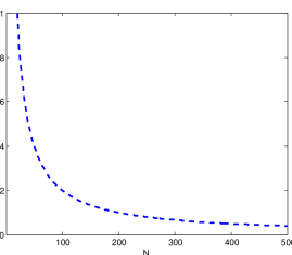
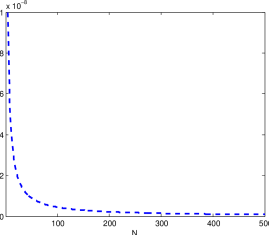
Figure 1 illustrates the convergence result of Corollary 5.3. All computations were made on an INTEL Core2Duo 2400MHz machine. We consider two scenarios: in case $(a)$ we have a favourable set of parameters for the ZCB valuation; in case $(b)$ we choose an unrealistic high of 20% for the interest rate market volatility and a time to maturity of 10 years. Within the Vasicek model the valuation is done according to the pricing formula (53). The approximative values $P(0,T;M,H)$ of the ZCB prices in the $\mathcal{E}(1/2,\lambda)$ model are computed according to Corallary 5.3 via (48) with $M=10$ and $H=30.$ In both cases we observe fast convergence of the respective prices.

(a) Favourable case

(b) Unfavourable case

Figure 1: Relative price errors against $N$ approximating ZCB prices $P(0,T)$ in the Vasicek model by $P^{(N)}(0,T;10,30)$ in the $\mathcal{E}(1/2,\lambda)$ model via (48) in two scenarios: $(a)\ \text{Vasicek model with }a=0.2,\,\sigma=0.05,\,T=1\text{ year},\,\theta=8\%,$ and $r_{0}=5\%$; $(b)\ \text{Vasicek model with }a=0.2,\,\sigma=0.2,\,T=10\text{ years},\,\theta=8\%,$ and $r_{0}=5\%$.

Furthermore, we see that the choice of the truncating parameters $M=10$ and $H=30$ is satisfactory for our purpose. The computation time of one ZCB price via (48) is less than 0.1 seconds. Similar computation in the $\mathcal{E}(p,\lambda)$ model according to (47) takes 2.67 seconds.

6 Discussion

In this section we discuss the advantages of the $\mathcal{E}(p,\lambda)$ model with respect to the positivity of the interest rates. We use the case study of a ZCB valuation, showing that the $\mathcal{E}(p,\lambda)$ model can still be used when the Vasicek model reaches its limits.

The main shortcoming of all models with Gaussian distribution, including the Vasicek model, is the positive probability of the interest rates becoming negative. Although this probability is rather small, some problems may appear while valuing ZCBs with long residual maturity. For instance, Rogers [15] illustrates how an attempt to keep the probability of negative interest rates negligible by choosing suitable parameters of the Vasicek model in the limiting case $t\rightarrow\infty$ leads to an exponential growth in $t$ of the ZCB prices. Conversely, the $\mathcal{E}(p,\lambda)$ model allows the choice of the lower and upper bounds $r_{m}$ and $r_{M}$ for the interest rate, and excludes the possibility of negative as well as unrealistically high positive interest rates.

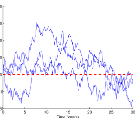
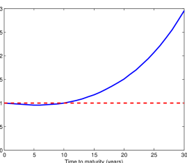
Times of financial crisis are often accompanied by interest rates near $0\%$, as we see at present. The following example of pricing ZCBs in a respective scenario illustrates the advantage of the $\mathcal{E}(p,\lambda)$ model over the Vasicek model. First, we assume the Vasicek model given according to (49) with $\theta=4\%,\ \sigma=0.05,\ k=0.1$ and $r(0)=1\%.$ Figure 2 $(a)$ shows three sample paths of the underlying process $(r_{t})_{t\geq 0}$ over a period of 30 years simulated according to (50). We see that every path of the simulated process spends some time below the zero mark. Figure 2 $(b)$ demonstrates the weakness of the model in the case at hand, as we observe that the ZCB prices are not monotone falling in the time to maturity and even exceed the upper bound of 1 monetary unit, which is contradictory to no-arbitrage principles.

(a) Short-rate

(b) ZCB prices

Figure 2: $(a)$ Three sample paths of the short-rate process (49) in the Vasicek model with $a=0.1,\,\theta=4\%,\,\sigma=0.05$ and $r(0)=1\%.$ $(b)$ ZCB prices in the Vasicek model with the given parameters and residual maturities from 1 to 30 years.

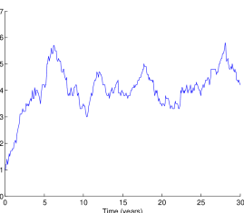
Now we consider the $\mathcal{E}(p,\lambda)$ model in a similar hypothetical setting. We set the lower and upper bounds at $r_{m}=0\%$ and $r_{M}=16\%$, and the state space discretization parameter $N=160.$ We choose $\lambda=1,\,\alpha=0.1$ and $\beta=0.3,$ in that we have with (24) a mean-reverting value of $4\%$ as in the case above. Here, we set $R_{0}=1\%$ as well. Figure 3 $(a)$ demonstrates a possible trajectory of the short-rate process $(R_{t})_{t\geq 0}$ over 30 years, simulated on the basis of the underlying distribution. In Figure 3 $(b)$ we see the strictly monotone decreasing character of the respective ZCB prices as a function of the time to maturity, which is highly plausible.

(a) Short-rate

(b) ZCB prices

Figure 3: $(a)$ A sample path of the short-rate process (21) in the $\mathcal{E}(p,\lambda)$ model with $\alpha=0.1,\,\beta=0.3,\,\lambda=1,\,r_{m}=0\%,\,r_{M}=16\%,\,N=160$ and $R_{0}=1\%.$ $(b)$ ZCB prices in the $\mathcal{E}(p,\lambda)$ model with the given parameters and residual maturities from 1 to 30 years.

7 Conclusions

This paper has explored a finite-state mean-reverting short-rate model based on the Ehrenfest process. The respective short-rate process can be seen as an affine linearly transformed birth-and-death process on $\{0,1,\cdots,N\},\ N\in\mathbb{N}.$ The model provides a certain degree of analytical tractability, since it allows explicit pricing of ZCBs and solves the problem of negative interest rates characteristic of Gaussian models. The pricing formulae for ZCBs have been derived for both the general case and the special case, in which the underlying distribution is symmetric with respect to the mean-reverting value. The key to both approaches has turned out to be the representation of the underlying Ehrenfest process as a sum of independent binary processes, which has been possible only in continuous time. We also used the hypergeometric functions of a matrix argument and the Krawtchouk polynomials. The special case benefits also from a more tractable pricing formula for ZCBs.

We have seen that the Ehrenfest short-rate model is a good approximation to the Vasicek model under normal conditions and a better alternative to it in extreme cases, where the interest rates are low and the volatility is high, providing solely positive interest rates. A further advantage of the model is the availability of five fitting parameters in the general case.

Our conclusion is that especially the general case of the Ehrenfest short-rate model is an interesting enrichment in the field of term structure modelling, combining analytical tractability with the desired property of interest rates remaining positive.

Problems that remain open for the short-rate model that we have examined here are the derivation of an explicit pricing formula for European options on ZCBs, parameter estimates for the model under the objective measure, and an extension of the model according to the three urn Ehrenfest model (see. [10], pp. 363 - 368).

References

• [1] Billingsley, P. (1968). Convergence of Probability Measures. John Wiley, New York.
• [2] Bingham, N. H. (1991). Fluctuation theory for the Ehrenfest urn. Adv. Appl. Prob. 23, 598–611.
• [3] Brémaud, P. (1999). Markov Chains: Gibbs Fields, Monte Carlo Simulation, and Queues. Springer, New York.
• [4] Brigo, D. and Mercurio, F. (2005). Interest Rate Models - Theory and Practice. Springer, Berlin.
• [5] Buehlmann, H. (1994). Continuous and discrete models in finance, in particular for stochastic interest rates. Riv. Mat. Sci. Econom. Social. 17, 3–20.
• [6] Delbaen, F. and Shirakawa, H. (2002). An interest rate model with upper and lower bounds. Asia-Pacific Finan. Markets 9, 191–209.
• [7] Gross, K. I. and Richards, D. St. P. (1989). Total positivity, spherical series, and hypergeometric functions of matrix argument. J. Approx. Theory 59, no. 2, 224–246.
• [8] Karlin, S. and Taylor, H. M. (1975). A First Course in Stochastic Processes, 2nd edn. Academic Press, New York.
• [9] Karlin, S. and Taylor, H. M. (1981). A Second Course in Stochastic Processes. Academic Press, New York.
• [10] Karlin, S. and McGregor, J. (1965). Ehrenfest urn models. J. Appl. Prob. 2, 352–376.
• [11] Koev, P. and Edelman, A. (2006). The efficient evaluation of the hypergeometric function of a matrix argument. Math. Comput. 75, 833–846.
• [12] Kraft, O. and Schaefer, M. (1993). Mean passage times for tridiagonal transition matrices and a two-parameter Ehrenfest urn model. J. Appl. Prob. 30, 964–970.
• [13] Lakner, P. (2006). Martingale measures for a class of right-continuous processes. Math. Finance 3, no. 1, 43–53.
• [14] Okunev, J. and Tippett, M. (1990). Continuous-time stochastic calculus: A survey of applications in finance and accountancy. IMA J. Math. Appl. Bus. Ind. 2, no. 2, 157–171.
• [15] Rogers, L. C. G. (1995). Which Model for Term Structure of Interest Rates Should One Use? In M. Davis, D. Duffie, W. Fleming and S. Shreve (eds.), Mathematical Finance. IMA Vol. Math. Appl. Vol. 65. Springer, New York.
• [16] Siegert, A. J. F. (1949). On the approach to statistical equlibrium. Phys. Rev. 71, 1708–1714.
• [17] Sumita, U., Gotoh, J. and Jin, H. (2006). Numerical exploration of dynamic behavior of Ornstein-Uhlenbeck process via Ehrenfest process approximation. J. Oper. Res. Japan 49, 256–278.
• [18] Szegö, G. (1983). Orthogonal Polynomials. Amer. Math. Soc. Colloquium Publ. 23, AMS. Providence, RI.
• [19] Takahashi, H. (2004). Ehrenfest model with large jumps in finance. Physica D 189, no. 1-2, 61–69.
• [20] Vasicek, O. (1977). An equilibrium characterisation of the term structure. J. Financ. Econ. 5, 177–188.
• [21] Voit, M. (1996). Asymptotic distributions for the Ehrenfest urn and related random walks. J. Appl. Prob. 33, no. 3, 340–356.