Introduction to the Basics of Heegaard Floer Homology

Abstract

This paper provides an introduction to the basics of Heegaard Floer homology with some emphasis on the hat theory and to the contact geometric invariants in the theory. The exposition is designed to be comprehensible to people without any prior knowledge of the subject.

1 Introduction

Heegaard Floer homology was introduced by Peter Ozsváth and Zoltan Szabó at the beginning of the new millennium. Since then it developed very rapidly due to its various contributions to low-dimensional topology, particularly knot theory and contact geometry. The present paper is designed to give an introduction to the basics of Heegaard Floer theory with some emphasis on the hat theory. We try to provide all details necessary to communicate a complete and comprehensible picture. We would like to remark that there already are introductory articles to this subject (see [21], [22] and [23]). The difference between the existing articles and the present article is threefold: First of all we present a lot more details. We hope that these details will provide a complete picture of the basics of the theory. Our goal is to focus on those only which are relevant for the understanding of Heegaard Floer homology. Secondly, our exposition is not designed to present any applications and, in fact, we do not present any. Explaining applications to the reader would lead us too far away from the basics and would force us to make some compromise to the exposition. We felt that going into advanced elements would be disturbing to the goal of this paper. And thirdly, we have a slight contact geometric focus.

We think that the reader will profit the most from this paper when reading it completely rather than selecting a few elements: We start with a low-paced exposition and gain velocity as we move on. In this way we circumvent the creation of too many redundancies and it enables us to focus on the important facts at each stage of the paper. We expect the reader to have some knowledge about algebraic topology and surgery theory. As standard references we suggest [1] and [7].
In §2 and §3 we start with Heegaard diagrams and introduce everything necessary to construct the homology theory. We included a complete discussion of the invariance of Heegaard Floer theory (cf. §4) for two reasons: Firstly, the isomorphisms defined for showing invariance appear very frequently in the research literature. Secondly, the proof is based on constructions which can be called the standard constructions of the theory. Those who are impatient may just read §4.4.1 and skip the rest of §4. However, the remainder of the article refers to details of §4 several times. The following paragraph, i.e. §5, is devoted to the knot theoretic variant of Heegaard Floer theory, called knot Floer homology. In §6 and §7 we outline how to assign to a $4$-dimensional cobordism a map between the Floer homologies of the boundary components and derive the surgery exact triangle. This triangle is one of the most important tools, particularly for the contact geometric applications. Finally, the article focuses on the definition of the contact geometric invariants.
We are aware of the fact that there is a lot of material missing in this article. However, the presented theory provides a solid groundwork for understanding of what we omitted. We would like to outline at least some of the missing material: First of all the homology groups as well as the cobordism maps refine with respect to $\mbox{\rm Spin}^{c}$-structures. We indicate this fact in §2 but do not outline any details. The standard reference is the article [17] of Ozsváth and Szabó. However, we suggest the reader first to familiarize with $\mbox{\rm Spin}^{c}$-structures, especially with their interpretation as homology classes of vector fields (cf. [28]). Furthermore, there is an absolute $\mathbb{Q}$-grading on these homology groups (see [19]) and in case of knot Floer homologies for homologically trivial knots an additional $\mathbb{Z}$-grading (see [14]). Both gradings carry topological information and may appear as a help in explicit calculations, especially in combination with the surgery exact triangles. The knot Floer homologies admit additional exact sequences besides the surgery exact sequence. An example is the skein exact sequence (see [14] and [24]). For contact geometric applications the adjunction inequalities play a central role as they give a criterion for the vanishing of cobordism maps (see [18] or cf. [25]). Going a bit further, there are other flavors of Heegaard Floer homology: András Juhasz defined the so-called Sutured Floer homology of sutured manifolds (see [12]) and Ozsváth, Lipshitz and Thurston defined a variant of Heegaard Floer homology for manifolds with parameterized boundary (see [9]).

2 Introduction to $\widehat{\mbox{\rm HF}}$ as a Model for Heegaard Floer Theory

2.1 Heegaard Diagrams

One of the major results of Morse theory is the development of surgery and handle decompositions. Morse theory captures the manifold’s topology in terms of a decomposition of it into topologically easy-to-understand pieces called handles (cf. [7]). In the case of closed $3$-manifolds the handle decomposition can be assumed to be very symmetric. This symmetry allows us to describe the manifold’s diffeomorphism type by a small amount of data. Heegaard diagrams are omnipresent in low-dimensional topology. Unfortunately there is no convention what precisely to call a Heegaard diagram; the definition of this notion underlies slight variations in different sources. Since Heegaard Floer Homology intentionally uses a non-efficient version of Heegaard diagrams, i.e. we fix more information than needed to describe the manifold’s type, we shortly discuss, what is to be understood as Heegaard diagram throughout this article.
A short summary of what we will discuss would be that we fix the data describing a handle decomposition relative to a splitting surface. Let $Y$ be a closed oriented $3$-manifold and $\Sigma\subset Y$ a splitting surface, i.e. a surface of genus $g$ such that $Y\backslash\Sigma$ decomposes into two handlebodies $H_{0}$ and $H_{1}$. We fix a handle decomposition of $\overline{Y\backslash H_{1}}$ relative to this splitting surface $\Sigma$, i.e. there are $2$-handles $h^{2}_{1,i}$, $i=1,\dots,g$, and a $3$-handle $h^{3}_{1}$ such that (cf. [7])

$$Y\backslash H_{1}\cong(\Sigma\times[0,1])\cup_{\partial}(h^{2}_{1,1}\cup_{\partial}\dots\cup_{\partial}h^{2}_{1,g}\cup_{\partial}h^{3}_{1}).$$ (2.1)

We can rebuild $Y$ from this by gluing in $2$-handles $h^{2}_{0,i}$, $i=1,\dots,g$, and a $3$-handle $h^{3}_{0}$. Hence, $Y$ can be written as

$$Y\cong(h^{3}_{0}\cup_{\partial}h^{2}_{0,1}\cup_{\partial}\dots\cup_{\partial}h^{2}_{0,g})\cup_{\partial}(\Sigma\times[0,1])\cup_{\partial}(h^{2}_{1,1}\cup_{\partial}\dots\cup_{\partial}h^{2}_{1,g}\cup_{\partial}h^{3}_{1}).$$ (2.2)

Collecting the data from this decomposition we obtain a triple $(\Sigma,\alpha,\beta)$ where $\Sigma$ is the splitting surface of genus $g$, $\alpha=\{\alpha_{1},\dots,\alpha_{g}\}$ are the images of the attaching circles of the $h^{2}_{0,i}$ interpreted as sitting in $\Sigma$ and $\beta=\{\beta_{1},\dots,\beta_{g}\}$ the images of the attaching circles of the $2$-handles $h^{2}_{1,i}$ interpreted as sitting in $\Sigma$. This will be called a Heegaard diagram of $Y$. Observe that these data determine a Heegaard decomposition in the classical sense by dualizing the $h^{2}_{0,i}$. Dualizing a $k$-handle $D^{k}\times D^{3-k}$ means to reinterpret this object as $D^{3-k}\times D^{k}$. Both objects are diffeomorphic but observe that the former is a $k$-handle and the latter a $(3-k)$-handle. Observe that the $\alpha$-curves are the co-cores of the $1$-handles in the dualized picture, and that sliding $h^{1}_{0,i}$ over $h^{1}_{0,j}$ means, in the dual picture, that $h^{2}_{0,j}$ is slid over $h^{2}_{0,i}$.

2.2 Introduction to $\widehat{\mbox{\rm HF}}$ — Topology and Analysis

Given a closed, oriented $3$-manifold $Y$, we fix a Heegaard diagram $(\Sigma,\alpha,\beta)$ of $Y$ as defined in §2.1. We can associate to it the triple $(\mbox{\rm Sym}^{g}(\Sigma),\mathbb{T}_{\alpha},\mathbb{T}_{\beta})$ which we will explain now:
By $\mbox{\rm Sym}^{g}(\Sigma)$ we denote the $g$-fold symmetric product of $\Sigma$, defined by taking the quotient under the canonical action of $S_{g}$ on $\Sigma^{\times g}$, i.e.

$$\mbox{\rm Sym}^{g}(\Sigma)=\Sigma^{\times g}/S_{g}.$$

Although the action of $S_{g}$ has fixed points, the symmetric product is a manifold. The local model is given by $\mbox{\rm Sym}^{g}(\mathbb{C})$ which itself can be identified with the set of normalized polynomials of degree $g$. An isomorphism is given by sending a point $[(p_{1},\ldots,p_{g})]$ to the normalized polynomial uniquely determined by the zero set $\{p_{1},\ldots,p_{g}\}$. Denote by

$$\pi\colon\thinspace\Sigma^{\times g}\longrightarrow\mbox{\rm Sym}^{g}(\Sigma)$$

the projection map.

The attaching circles $\alpha$ and $\beta$ define submanifolds

$$\mathbb{T}_{\alpha}=\alpha_{1}\times\ldots\times\alpha_{g}\;\;\mbox{\rm and }\;\;\mathbb{T}_{\beta}=\beta_{1}\times\ldots\times\beta_{g}$$

in $\Sigma^{\times g}$. Obviously, the projection $\pi$ embeds these into the symmetric product. In the following we will denote by $\mathbb{T}_{\alpha}$ and $\mathbb{T}_{\beta}$ the manifolds embedded into the symmetric product.

2.2.1 The chain complex

Define $\widehat{\mbox{\rm CF}}(\Sigma,\alpha,\beta)$ as the free $\mathbb{Z}$-module (or $\mathbb{Z}_{2}$-module) generated by the intersection points $\mathbb{T}_{\alpha}\cap\mathbb{T}_{\beta}$ inside $\mbox{\rm Sym}^{g}(\Sigma)$.

Definition 2.1.

A map $\phi$ of the $2$-disc $\mathbb{D}^{2}$ (regarded as the unit $2$-disc in $\mathbb{C}$) into the symmetric product $\mbox{\rm Sym}^{g}(\Sigma)$ is said to connect two points $x,y\in\mathbb{T}_{\alpha}\cap\mathbb{T}_{\beta}$ if

$$\phi(i) = x,$$

$$\phi(-i) = y,$$

$$\phi(\partial\mathbb{D}\cap\{z\in\mathbb{C}\,|\,Re(z)<0\}) \subset \mathbb{T}_{\alpha},$$

$$\phi(\partial\mathbb{D}\cap\{z\in\mathbb{C}\,|\,Re(z)>0\}) \subset \mathbb{T}_{\beta}.$$

Continuous mappings of the $2$-disc into the symmetric product $\mbox{\rm Sym}^{g}(\Sigma)$ that connect two intersection points $x,y\in\mathbb{T}_{\alpha}\cap\mathbb{T}_{\beta}$ are called Whitney discs. The set of homotopy classes of Whitney discs connecting $x$ and $y$ is denoted by $\pi_{2}(x,y)$ in case $g>2$.

In case $g\leq 2$ we have to define the object $\pi_{2}(x,y)$ slightly different. However, we can always assume, without loss of generality, that $g>2$ and, thus, we will omit discussing this case at all. We point the interested reader to [17].
Fixing a point $z\in\Sigma\backslash(\alpha\cup\beta)$, we can construct a differential

$$\widehat{\partial}_{z}\colon\thinspace\widehat{\mbox{\rm CF}}(\Sigma,\alpha,\beta)\longrightarrow\widehat{\mbox{\rm CF}}(\Sigma,\alpha,\beta)$$

by defining it on the generators of $\widehat{\mbox{\rm CF}}(\Sigma,\alpha,\beta)$. Given a point $x\in\mathbb{T}_{\alpha}\cap\mathbb{T}_{\beta}$, we define $\widehat{\partial}_{z}x$ to be a linear combination

$$\widehat{\partial}_{z}x=\sum_{y\in\mathbb{T}_{\alpha}\cap\mathbb{T}_{\beta}}\left.\widehat{\partial}_{z}x\right|_{y}\cdot y$$

of all intersection points $y\in\mathbb{T}_{\alpha}\cap\mathbb{T}_{\beta}$. The definition of the coefficients will occupy the remainder of this paragraph. The idea resembles other Floer homology theories. The goal is to define $\left.\widehat{\partial}_{z}x\right|_{y}$ as a signed count of holomorphic Whitney discs connecting $x$ and $y$ which are rigid up to reparametrization. First we have to introduce almost complex structures into this picture. A more detailed discussion of these will be given in §2.3. For the moment it will be sufficient to say that we choose a generic path $(\mathcal{J}_{s})_{s\in[0,1]}$ of almost complex structures on the symmetric product. Identifying the unit disc, after taking out the points $\pm i$, in $\mathbb{C}$ with $[0,1]\times\mathbb{R}$ we define $\phi$ to be holomorphic if it satisfies for all $(s,t)\in[0,1]\times\mathbb{R}$ the equation

$$\frac{\partial\phi}{\partial s}(s,t)+\mathcal{J}_{s}\bigl{(}\frac{\partial\phi}{\partial t}(s,t)\bigr{)}=0.$$ (2.3)

Looking into $(\ref{holomeq})$ it is easy to see that a holomorphic Whitney disc $\phi$ can be reparametrized by a constant shift in $\mathbb{R}$-direction without violating $(\ref{holomeq})$.

Definition 2.2.

Given two points $x,y\in\mathbb{T}_{\alpha}\cap\mathbb{T}_{\beta}$, we denote by $\mathcal{M}_{\mathcal{J}_{s}}(x,y)$ the set of holomorphic Whitney discs connecting $x$ and $y$. We call this set moduli space of holomorphic Whitney discs connecting $x$ and $y$. Given a homotopy class $[\phi]\in\pi_{2}(x,y)$, denote by $\mathcal{M}_{\mathcal{J}_{s},[\phi]}$ the space of holomorphic representatives in the homotopy class of $\phi$.

In the following the generic path of almost complex structures will not be important and thus we will suppress it from the notation. Since the path is chosen generically (cf. §2.3 or see [17]) the moduli spaces are manifolds. The constant shift in $\mathbb{R}$-direction induces a free $\mathbb{R}$-action on the moduli spaces. Thus, if $\mathcal{M}_{[\phi]}$ is non-empty its dimension is greater than zero. We take the quotient of $\mathcal{M}_{[\phi]}$ under the $\mathbb{R}$-action and denote the resulting spaces by

$$\widehat{\mathcal{M}}_{[\phi]}=\mathcal{M}_{[\phi]}/\mathbb{R}\;\;\mbox{\rm and}\;\;\widehat{\mathcal{M}}(x,y)=\mathcal{M}(x,y)/\mathbb{R}.$$

The so-called signed count of $0$-dimensional components of $\widehat{\mathcal{M}}(x,y)$ means in case of $\mathbb{Z}_{2}$-coefficients simply to count mod $2$. In case of $\mathbb{Z}$-coefficients we have to introduce coherent orientations on the moduli spaces. We will roughly sketch this process in the following.
Obviously, in case of $\mathbb{Z}$-coefficients we cannot simply count the $0$-dimensional components of $\widehat{\mathcal{M}}(x,y)$. The defined morphism would not be a differential. To circumvent this problem we have to introduce signs appropriately attached to each component. The $0$-dimensional components of $\widehat{\mathcal{M}}(x,y)$ correspond to the $1$-dimensional components of $\mathcal{M}(x,y)$. Each of these components carries a canonical orientation induced by the free $\mathbb{R}$-action given by constant shifts. We introduce orientations on these components. Comparing the artificial orientations with the canonical shifting orientation we can associate to each component, i.e. each element in $\widehat{\mathcal{M}}(x,y)$, a sign. The signed count will respect the signs attached. There is a technical condition called coherence (see [17] or cf. §2.3) one has to impose on the orientations. This technical condition ensures that the morphism $\widehat{\partial}_{z}$ is a differential.
The chosen point $z\in\Sigma\backslash(\alpha\cup\beta)$ will be part of the definition. The path $(\mathcal{J}_{s})_{s\in[0,1]}$ is chosen in such a way that

$$V_{z}=\{z\}\times\mbox{\rm Sym}^{g-1}(\Sigma)\hookrightarrow\mbox{\rm Sym}^{g}(\Sigma)$$

is a complex submanifold. For a Whitney disc (or its homotopy class) $\phi$ define $n_{z}(\phi)$ as the intersection number of $\phi$ with the submanifold $V_{z}$. We define

$$\left.\widehat{\partial}_{z}x\right|_{y}=\#\widehat{\mathcal{M}}(x,y)^{0}_{n_{z}=0},$$

i.e. the signed count of the $0$-dimensional components of the unparametrized moduli spaces of holomorphic Whitney discs connecting $x$ and $y$ with the property that their intersection number $n_{z}$ is trivial.

Theorem 2.3 (see [17]).

The assignment $\widehat{\partial}_{z}$ is well-defined.

Theorem 2.4 (see [17]).

The morphism $\widehat{\partial}_{z}$ is a differential.

We will give sketches of the proofs of the last two theorems later in §2.3. At the moment we do not know enough about Whitney discs and the symmetric product to prove it.

Definition 2.5.

We denote by $\widehat{\mbox{\rm CF}}(\Sigma,\alpha,\beta,z)$ the chain complex given by the data $(\widehat{\mbox{\rm CF}}(\Sigma,\alpha,\beta),\partial_{z})$. Denote by $\widehat{\mbox{\rm HF}}(Y)$ the induced homology theory $H_{*}(\widehat{\mbox{\rm CF}}(\Sigma,\alpha,\beta),\partial_{z})$.

The notation should indicate that the homology theory does not depend on the data chosen. It is a topological invariant of the manifold $Y$, although this is not the whole story. The theory depends on the choice of coherent system of orientations. For a manifold $Y$ there are $2^{b_{1}(Y)}$ numbers of non-equivalent systems of coherent orientations. The resulting homologies can differ (see Example 2.2). Nevertheless the orientations are not written down. We guess there are two reasons: The first would be that most of the time it is not really important which system is chosen. All reasonable constructions will work for every coherent orientation system, and in case there is a specific choice needed this will be explicitly stated. The second reason would be that it is possible to give a convention for the choice of coherent orientation systems. Since we have not developed the mathematics to state the convention precisely we point the reader to Theorem 2.31.

2.2.2 On Holomorphic Discs in the Symmetric Product

In order to be able to discuss a first example we briefly introduce some properties of the symmetric product.

Definition 2.6.

For a Whitney disc $\phi$ we denote by $\mu(\phi)$ the formal dimension of $\mathcal{M}_{\phi}$. We also call $\mu(\phi)$ the Maslov index of $\phi$.

For the readers that have not heard anything about Floer homology at all, just think of $\mu(\phi)$ as the dimension of the space $\mathcal{M}_{\phi}$, although even in case $\mathcal{M}_{\phi}$ is not a manifold the number $\mu(\phi)$ is defined (cf. §2.3). Just to give some intuition, note that the moduli spaces are the zero-set of a section, $S$ say, in a Banach bundle one associates to the given setup. The linearization of this section at the zero set is a Fredholm operator. Those operators carry a property called Fredholm index. The number $\mu$ is the Fredholm index of that operator. Even if the moduli spaces are no manifolds this number is defined. It is called formal dimension or expected dimension since in case the section $S$ intersects the zero-section of the Banach-bundle transversely (and hence the moduli spaces are manifolds) the Fredholm index $\mu$ equals the dimension of the moduli spaces. So, negative indices are possible and make sense in some situations. One can think of negative indices as the number of missing degrees of freedom to give a manifold.

Lemma 2.7.

In case $g(\Sigma)>2$ the 2nd homotopy group $\pi_{2}(\mbox{\rm Sym}^{g}(\Sigma))$ is isomorphic to $\mathbb{Z}$. It is generated by an element $S$ with $\mu(S)=2$ and $n_{z}(S)=1$, where $n_{z}$ is defined the same way as it was defined for Whitney discs.

Let $\eta\colon\thinspace\Sigma\longrightarrow\Sigma$ be an involution such that $\Sigma/\eta$ is a sphere. The map

$$\mathbb{S}^{2}\longrightarrow\mbox{\rm Sym}^{g}(\Sigma),\,\;y\longmapsto\{(y,\eta(y),y,\dots,y)\}$$

is a representative of $S$. Using this representative it is easy to see that $n_{z}(S)=1$. It is a property of $\mu$ as an index that it behaves additive under concatenation. Indeed the intersection number $n_{z}$ behaves additive, too. To develop some intuition for the holomorphic spheres in the symmetric product we state the following result from [17].

Lemma 2.8 (see [17]).

There is an exact sequence

$$0\longrightarrow\pi_{2}(\mbox{\rm Sym}^{g}(\Sigma))\longrightarrow\pi_{2}(x,x)\longrightarrow\mbox{\rm ker}(n_{z})\longrightarrow 0.$$

The map $n_{z}$ provides a splitting for the sequence.

Observe that we can interpret a Withney disc in $\pi_{2}(x,x)$ as a family of paths in $\mbox{\rm Sym}^{g}(\Sigma)$ based at the constant path $x$. We can also interpret an element in $\pi_{2}(\mbox{\rm Sym}^{g}(\Sigma))$ as a family of paths in $\mbox{\rm Sym}^{g}(\Sigma)$ based at the constand path $x$. Interpreted in this way there is a natural map from $\pi_{2}(\mbox{\rm Sym}^{g}(\Sigma))$ into $\pi_{2}(x,x)$. The map $n_{z}$ provides a splitting for the sequence as it may be used to define the map

$$\pi_{2}(x,x)\longrightarrow\pi_{2}(\mbox{\rm Sym}^{g}(\Sigma))$$

sending a Whitney disc $\phi$ to $n_{z}(\phi)\cdot S$. This obviously defines a splitting for the sequence.

Lemma 2.9.

The Kernel of $n_{z}$ interpreted as a map on $\pi_{2}(x,x)$ is isomorphic to $H^{1}(Y;\mathbb{Z})$.

With the help of concatenation we are able to define an action

$$*\colon\thinspace\pi_{2}(x,x)\times\pi_{2}(x,y)\longrightarrow\pi_{2}(x,y),$$

which is obviously free and transitive. Thus, we have an identification

$$\begin{diagram}$$ (2.4)

as principal bundles over a one-point space, which is another way of saying that the concatenation action endows $\pi_{2}(x,y)$ with a group structure after fixing a unit element in $\pi_{2}(x,y)$. To address the well-definedness of $\widehat{\partial}_{z}$ we have to show that the sum in the definition of $\widehat{\partial}_{z}$ is finite. For the moment let us assume that for a generic choice of path $(\mathcal{J}_{s})_{s\in[0,1]}$ the moduli spaces $\widehat{\mathcal{M}}_{\phi}$ with $\mu(\phi)=1$ are compact manifolds (cf. Theorem 2.22), hence their signed count is finite. Assuming this property we are able to show well-definedness of $\widehat{\partial}_{z}$ in case $Y$ is a homology sphere.

Proof of Theorem 2.3 for $b_{1}(Y)=0$.

Observe that

$$\widehat{\mathcal{M}}(x,y)^{0}_{n_{z}=0}=\bigsqcup_{\phi\in H(x,y,1)}\widehat{\mathcal{M}}_{\phi},$$ (2.5)

where $H(x,y,1)\subset\pi_{2}(x,y)$ is the subset of homotopy classes admitting holomorphic representatives with $\mu(\phi)=1$ and $n_{z}=0$. We have to show that $H(x,y,1)$ is a finite set. Since $b_{1}(Y)=0$ the cohomology $H^{1}(Y;\mathbb{Z})$ vanishes. By our preliminary discussion, given a reference disc $\phi_{0}\in\pi_{2}(x,y)$, any $\phi_{xy}\in\pi_{2}(x,y)$ can be written as a concatenation $\phi_{xy}=\phi*\phi_{0}$, where $\phi$ is an element in $\pi_{2}(x,x)$. Since we are looking for discs with index one we have to find all $\phi\in\pi_{2}(x,x)$ satisfying the property $\mu(\phi)=1-\mu(\phi_{0})$. Recall that $Y$ is a homology sphere and thus $\pi_{2}(x,x)\cong\mathbb{Z}\otimes\{S\}$. Hence, the disc $\phi$ is described by an integer $k\in\mathbb{Z}$, i.e. $\phi=k\cdot S$. The property $\mu(S)=2$ tells us that

$$1-\mu(\phi_{0})=\mu(\phi)=\mu(k\cdot S)=k\cdot\mu(S)=2k.$$

There is at most one $k\in\mathbb{Z}$ satisfying this equation, so there is at most one homotopy class of Whitney discs satisfying the property $\mu=1$ and $n_{z}=0$. ∎

In case $Y$ has non-trivial first cohomology we need an additional condition to make the proof work. The given argument obviously breaks down in this case. To fix this we impose a topological/algebraic condition on the Heegaard diagram. Before we can define these admissibility properties we have to go into the theory a bit more.
There is an obstruction to finding Whitney discs connecting two given intersection points $x,y$. The two points $x$ and $y$ can certainly be connected via paths inside $\mathbb{T}_{\alpha}$ and $\mathbb{T}_{\beta}$. Fix two paths $a\colon\thinspace I\longrightarrow\mathbb{T}_{\alpha}$ and $b\colon\thinspace I\longrightarrow\mathbb{T}_{\beta}$ such that $-\partial b=\partial a=y-x$. This is the same as saying we fix a closed curve $\gamma_{xy}$ based at $x$, going to $y$ along $\mathbb{T}_{\alpha}$, and moving back to $x$ along $\mathbb{T}_{\beta}$. Obviously $\gamma_{xy}=b+a$. Is it possible to extend the curve $\gamma_{xy}$, after possibly homotoping it a bit, to a disc? If so, this would be a Whitney disc. Thus, finding an obstruction can be reformulated as: Is $[\gamma_{xy}]=0\in\pi_{1}(\mbox{\rm Sym}^{g}(\Sigma))$?

Lemma 2.10 (see [17]).

The group $\pi_{1}(\mbox{\rm Sym}^{g}(\Sigma))$ is abelian.

Given a closed curve $\gamma\subset\mbox{\rm Sym}^{g}(\Sigma)$ in general position (i.e. not meeting the diagonal of $\mbox{\rm Sym}^{g}(\Sigma)$), we can lift this curve to

$$(\gamma_{1},\dots,\gamma_{g})\colon\thinspace\mathbb{S}^{1}\longrightarrow\Sigma^{\times g}.$$

Projection onto each factor $\Sigma$ defines a $1$-cycle. We define

$$\Phi(\gamma)=\gamma_{1}+\dots+\gamma_{g}.$$

Lemma 2.11 (see [17]).

The map $\Phi$ induces an isomorphism

$$\Phi_{*}\colon\thinspace H_{1}(\mbox{\rm Sym}^{g}(\Sigma))\longrightarrow H_{1}(\Sigma;\mathbb{Z}).$$

By surgery theory (see [7], p.​ 111) we know that

$$\frac{H_{1}(\Sigma;\mathbb{Z})}{[\alpha_{1}],\ldots,[\alpha_{g}],[\beta_{1}],\ldots,[\beta_{g}]}\cong H_{1}(Y;\mathbb{Z})$$ (2.6)

The curve $\gamma_{xy}$ is homotopically trivial in the symmetric product if and only if $\Phi_{*}([\gamma_{xy}])$ is trivial. If we pick different curves $a$ and $b$ to define another curve $\eta_{xy}$, the difference

$$\Phi(\gamma_{xy})-\Phi(\eta_{xy})$$

is a sum of $\alpha$-and $\beta$-curves. Thus, interpreted as a cycle in $H_{1}(Y;\mathbb{Z})$, the class

$$[\Phi(\gamma_{xy})]\in H_{1}(Y;\mathbb{Z})$$

does not depend on the choices made in its definition. We get a map

$$\begin{array}[]{rccl}\epsilon\colon\thinspace&(\mathbb{T}_{\alpha}\cap\mathbb{T}_{\beta})^{\times 2}&\longrightarrow&H_{1}(Y;\mathbb{Z})\\ &(x,y)&\longmapsto&[\Phi(\gamma_{xy})]_{H_{1}(Y;\mathbb{Z})}\end{array}$$

with the following property.

Lemma 2.12.

If $\epsilon(x,y)$ is non-zero the set $\pi_{2}(x,y)$ is empty.

Proof.

Suppose there is a connecting disc $\phi$ then with $\gamma_{xy}=\partial(\phi(\mathbb{D}^{2}))$ we have

$$\epsilon(x,y)=[\Phi(\gamma_{xy})]_{H_{1}(Y;\mathbb{Z})}=\frac{\Phi_{*}([\gamma_{xy}]_{H_{1}({\tiny\mbox{\rm Sym}^{g}(\Sigma)})})}{[\alpha_{1}],\ldots,[\alpha_{g}],[\beta_{1}],\ldots,\beta_{g}]}=0$$

since $[\gamma_{xy}]_{\pi_{1}({\tiny\mbox{\rm Sym}^{g}(\Sigma)})}=0$. ∎

As a consequence we can split up the chain complex $\widehat{\mbox{\rm CF}}(\Sigma,\alpha,\beta,z)$ into subcomplexes. It is important to notice that there is a map

$$s_{z}\colon\thinspace\mathbb{T}_{\alpha}\cap\mathbb{T}_{\beta}\longrightarrow\mbox{\rm Spin}^{c}_{3}(Y)\cong H^{2}(Y;\mathbb{Z}),$$ (2.7)

such that $\mbox{\rm PD}(\epsilon(x,y))=s_{z}(x)-s_{z}(y)$. We point the reader interested in the definition of $s_{z}$ to [17]. Thus, fixing a $\mbox{\rm Spin}^{c}$-structure $s$, the $\mathbb{Z}$-module (or $\mathbb{Z}_{2}$-module) $\widehat{\mbox{\rm CF}}(\Sigma,\alpha,\beta,z;s)$ generated by $(s_{z})^{-1}(s)$ defines a subcomplex of $\widehat{\mbox{\rm CF}}(\Sigma,\alpha,\beta,z)$. The associated homology is denoted by $\widehat{\mbox{\rm HF}}(Y,s)$, and it is a submodule of $\widehat{\mbox{\rm HF}}(Y)$. Especially note that

$$\widehat{\mbox{\rm HF}}(Y)=\bigoplus_{s\in{\tiny\mbox{\rm Spin}^{c}_{3}}(Y)}\widehat{\mbox{\rm HF}}(Y,s).$$

Since $\mathbb{T}_{\alpha}\cap\mathbb{T}_{\beta}$ consists of finitely many points, there are just finitely many groups in this splitting which are non-zero. In general this splitting will depend on the choice of base-point. If $z$ is chosen in a different component of $\Sigma\backslash\{\alpha\cup\beta\}$ there will be a difference between the $\mbox{\rm Spin}^{c}$-structure associated to an intersection point. For details we point to [17].

Example 2.1.

The Heegaard diagram given by the data $(T^{2},\{\mu\},\{\lambda\})$ (cf. §2.1) is the $3$-sphere. To make use of Lemma 2.7 we add two stabilizations to get a Heegaard surface of genus $3$, i.e.

$$D=(T^{2}\#T^{2}\#T^{2},\{\mu_{1},\mu_{2},\mu_{3}\},\{\lambda_{1},\lambda_{2},\lambda_{3}\}),$$

where $\mu_{i}$ are meridians of the tori, and $\lambda_{i}$ are longitudes. The complement of the attaching curves is connected. Thus, we can arbitrarily choose the base point $z$. The chain complex $\widehat{\mbox{\rm CF}}(D,z)$ equals one copy of $\mathbb{Z}$ since it is generated by one single intersection point which we denote by $x$. We claim that $\widehat{\partial}_{z}x=0$. Denote by $[\phi]$ a homotopy class of Whitney discs connecting $x$ with itself. This is a holomorphic sphere which can be seen with Lemma 2.8, Lemma 2.9 and the fact that $H^{1}(\mathbb{S}^{3})=0$. By Lemma 2.7 the set $\pi_{2}(\mbox{\rm Sym}^{g}(\Sigma))$ is generated by $S$ with the property $n_{z}(S)=1$. The additivity of $n_{z}$ under concatenation shows that $[\phi]$ is a trivial holomorphic sphere and $\mu([\phi])=0$. Thus, the space $\mathcal{M}(x,x)^{1}_{n_{z}=0}$, i.e. the space of holomorphic Whitney discs connecting $x$ with itself, with $\mu=1$ and $n_{z}=0$, is empty. Hence

$$\widehat{\mbox{\rm HF}}(\mathbb{S}^{3})\cong\mathbb{Z}.$$

2.2.3 A Low-Dimensional Model for Whitney Discs

The exact sequence in Lemma 2.8 combined with Lemma 2.9 and $(\ref{pbident})$ gives an interpretation of Whitney discs as homology classes. Given a disc $\phi$, we define its associated homology class by $\mathcal{H}(\phi)$, i.e.

$$0\longrightarrow\pi_{2}(\mbox{\rm Sym}^{g}(\Sigma))\longrightarrow\pi_{2}(x,x)\overset{\mathcal{H}}{\longrightarrow}H_{2}(Y;\mathbb{Z})\longrightarrow 0.$$ (2.8)

In the following we intend to give a description of the map $\mathcal{H}$. Given a Whitney disc $\phi$, we can lift this disc to a map $\widetilde{\phi}$ by pulling back the branched covering $\pi$ (cf. diagram (2.9)).

$$\begin{diagram}$$ (2.9)

Let $S_{g-1}\subset S_{g}$ be the subgroup of permutations fixing the first component. Modding out $S_{g-1}$ we obtain the map $\overline{\phi}$ pictured in (2.9). Composing it with the projection onto the surface $\Sigma$ we define a map

$$\widehat{\phi}\colon\thinspace\widehat{\mathbb{D}}\longrightarrow\Sigma.$$

The image of this map $\widehat{\phi}$ defines what is called a domain.

Definition 2.13.

Denote by $\mathcal{D}_{1},\ldots,\mathcal{D}_{m}$ the closures of the components of the complement of the attaching circles $\Sigma\backslash\{\alpha\cup\beta\}$. Fix one point $z_{i}$ in each component. A domain is a linear combination

$$\mathcal{A}=\sum_{i=1}^{m}\lambda_{i}\cdot\mathcal{D}_{i}$$

with $\lambda_{1},\ldots,\lambda_{m}\in\mathbb{Z}$.

For a Whitney disc $\phi$ we define its associated domain by

$$\mathcal{D}(\phi)=\sum_{i=1}^{m}n_{z_{i}}(\phi)\cdot\mathcal{D}_{i}.$$

The map $\widehat{\phi}$ and $\mathcal{D}(\phi)$ are related by the equation

$$\widehat{\phi}(\widehat{\mathbb{D}})=\mathcal{D}(\phi)$$

as chains in $\Sigma$ relative to the set $\alpha\cup\beta$. We define $\mathcal{H}(\phi)$ as the associated homology class of $\widehat{\phi}_{*}[\widehat{\mathbb{D}}]$ in $H_{2}(Y;\mathbb{Z})$. The correspondence is given by closing up the boundary components by using the core discs of the $2$-handles represented by the $\alpha$-curves and the $\beta$-curves.

Lemma 2.14.

Two Whitney discs $\phi_{1},\phi_{2}\in\pi_{2}(x,x)$ are homotopic if and only if their domains are equal.

Proof.

Given two discs $\phi_{1}$, $\phi_{2}$ whose domains are equal, by definition $\mathcal{H}(\phi_{1})=\mathcal{H}(\phi_{2})$. By $(\ref{nice})$ they can only differ by a holomorphic sphere, i.e. $\phi_{1}=\phi_{2}+k\cdot S$. The equality $\mathcal{D}(\phi_{1})=\mathcal{D}(\phi_{2})$ implies that $n_{z}(\phi_{1})=n_{z}(\phi_{2})$. The equation

$$0=n_{z}(\phi_{2})-n_{z}(\phi_{1})=n_{z}(\phi_{2})-n_{z}(\phi_{2}+k\cdot S)=2k$$

forces $k$ to vanish. ∎

The interpretation of Whitney discs as domains is very useful in computations, as it provides a low-dimensional model. The symmetric product is $2g$-dimensional, thus an investigation of holomorphic discs is very inconvenient. However, not all domains are carried by holomorphic discs. Obviously, the equality $[\mathcal{D}(\phi)]=\widehat{\phi}_{*}[\widehat{\mathbb{D}}]$ connects the boundary conditions imposed on Whitney discs to boundary conditions of the domains. It is not hard to observe that the definition of $\widehat{\phi}$ follows the same lines as the construction of the isomorphism $\Phi_{*}$ of homology groups discussed earlier (cf. Lemma 2.11). Suppose we have fixed two intersections $x=\{x_{1},\dots,x_{g}\}$ and $y=\{y_{1},\dots,y_{g}\}$ connected by a Whitney disc $\phi$. The boundary $\partial(\phi(\mathbb{D}^{2}))$ defines a connecting curve $\gamma_{xy}$. It is easy to see that

$$\mbox{\rm im}(\left.\widehat{\phi}\right|_{\partial\widehat{\mathbb{D}}})=\Phi(\gamma_{xy})=\gamma_{1}+\dots+\gamma_{g}.$$

Restricting the $\gamma_{i}$ to the $\alpha$-curves we get a chain connecting the set $x_{1},\dots,x_{g}$ with $y_{1},\dots,y_{g}$, and restricting the $\gamma_{i}$ to the $\beta$-curves we get a chain connecting the set $y_{1},\dots,y_{g}$ with $x_{1},\dots,x_{g}$. This means each boundary component of $\widehat{\mathbb{D}}$ consists of a set of arcs alternating through $\alpha$-curves and $\beta$-curves.

Definition 2.15.

A domain is called periodic if its boundary is a sum of $\alpha$-and $\beta$-curves and $n_{z}(\mathcal{D})=0$, i.e. the multiplicity of $\mathcal{D}$ at the domain $\mathcal{D}_{z}$ containing $z$ vanishes.

Of course a Whitney disc is called periodic if its associated domain is a periodic domain. The subgroup of periodic classes in $\pi_{2}(x,x)$ is denoted by $\Pi_{x}$.

Theorem 2.16 (see [17]).

For a $\mbox{\rm Spin}^{c}$-structure $s$ and a periodic class $\phi\in\Pi_{x}$ we have the equality

$$\mu(\phi)=\left<c_{1}(s),\mathcal{H}(\phi)\right>.$$

This is a deep result connecting the expected dimension of a periodic disc with a topological property. Note that, because of the additivity of the expected dimension $\mu$, the homology groups $\widehat{\mbox{\rm HF}}(Y,s)$ can be endowed with a relative grading defined by

$$\mbox{\rm gr}(x,y)=\mu(\phi)-2\cdot n_{z}(\phi),$$

where $\phi$ is an arbitrary element of $\pi_{2}(x,y)$. In the case of homology spheres this defines a relative $\mathbb{Z}$-grading because by Theorem 2.16 the expected dimension vanishes for all periodic discs. In case of non-trivial homology they just vanish modulo $\delta(s)$, where

$$\delta(s)=\underset{A\in H_{2}(Y;\mathbb{Z})}{\mbox{\rm gcd}}\left<c_{1}(s),A\right>,$$

i.e. it defines a relative $\mathbb{Z}_{\delta(s)}$-grading.

Definition 2.17.

A pointed Heegaard diagram $(\Sigma,\alpha,\beta,z)$ is called weakly admissible for the $\mbox{\rm Spin}^{c}$-structure $s$ if for every non-trivial periodic domain $\mathcal{D}$ such that $\left<c_{1}(s),\mathcal{H}(\mathcal{D})\right>=0$ the domain has positive and negative coefficients.

With this technical condition imposed the $\widehat{\partial}_{z}$ is a well-defined map on the subcomplex $\widehat{\mbox{\rm CF}}(\Sigma,\alpha,\beta,s)$. From admissibility it follows that for every $x,y\in(s_{z})^{-1}(s)$ and $j,k\in\mathbb{Z}$ there exists just a finite number of $\phi\in\pi_{2}(x,y)$ with $\mu(\phi)=j$, $n_{z}(\phi)=k$ and $\mathcal{D}(\phi)\geq 0$. The last condition means that all coefficients in the associated domain are greater or equal to zero.

Proof of Theorem 2.3 for $b_{1}(Y)\not=0$.

Recall that holomorphic discs are either contained in a complex submanifold $C$ or they intersect $C$ always transversely and always positive. The definition of the path $(\mathcal{J}_{s})_{s\in[0,1]}$ (cf. §2.3) includes that all the $\{z_{i}\}\times\mbox{\rm Sym}^{g-1}(\Sigma)$ are complex submanifolds. Thus, holomorphic Whitney discs always satisfy $\mathcal{D}(\phi)\geq 0$. ∎

We close this paragraph with a statement that appears to be useful for developing intuition for Whitney discs. It helps imagining the strong connection between the discs and their associated domains.

Theorem 2.18 (see [17]).

Consider a domain $\mathcal{D}$ whose coefficients are all greater than or equal to zero. There exists an oriented $2$-manifold $S$ with boundary and a map $\phi\colon\thinspace S\longrightarrow\Sigma$ with $\phi(S)=\mathcal{D}$ with the property that $\phi$ is nowhere orientation-reversing and the restriction of $\phi$ to each boundary component of $S$ is a diffeomorphism onto its image.

2.3 The Structure of the Moduli Spaces

The material in this paragraph is presented without any details. The exposition pictures the bird’s eye view of the material. Recall from the last paragraphs that we have to choose a path of almost complex structures appropriately to define Heegaard Floer theory. So, a discussion of these structures is inevitable. However, a lot of improvements have been made the last years and we intend to mention some of them.
Let $(j,\eta)$ be a Kähler structure on the Heegaard surface $\Sigma$, i.e. $\eta$ is a symplectic form and $j$ an almost-complex structure that tames $\eta$. Let $z_{1},\dots,z_{m}$ be points, one in each component of $\Sigma\backslash\{\alpha\cup\beta\}$. Denote by $V$ an open neighborhood in $\mbox{\rm Sym}^{g}(\Sigma)$ of

$$D\cup\bigl{(}\bigcup_{i=1}^{m}\{z_{i}\}\times\mbox{\rm Sym}^{g-1}(\Sigma)\bigr{)},$$

where $D$ is the diagonal in $\mbox{\rm Sym}^{g}(\Sigma)$.

Definition 2.19.

An almost complex structure $J$ on $\mbox{\rm Sym}^{g}(\Sigma)$ is called $(j,\eta,V)$-nearly symmetric if $J$ agrees with $sym^{g}(j)$ over $V$ and if $J$ tames $\pi_{*}(\eta^{\times g})$ over $\overline{V}^{c}$. The set of $(j,\eta,V)$-nearly symmetric almost-complex structures will be denoted by $\mathcal{J}(j,\eta,V)$.

The almost complex structure $sym^{g}(j)$ on $\mbox{\rm Sym}^{g}(\Sigma)$ is the natural almost complex structure induced by the structure $j$. Important for us is that the structure $J$ agrees with $sym^{g}(j)$ on $V$. This makes the $\{z_{i}\}\times\mbox{\rm Sym}^{g-1}(\Sigma)$ complex submanifolds with respect to $J$. This is necessary to guarantee positive intersections with Whitney discs. Without this property the proof of Theorem 2.3 would break down in the case the manifold has non-trivial topology.
We are interested in holomorphic Whitney discs, i.e. discs in the symmetric product which are solutions of (2.3). Denote by the $\partial_{\mathcal{J}_{s}}$ the Cauchy-Riemann type operator defined by equation (2.3). Define $\mathcal{B}(x,y)$ as the space of Whitney discs connecting $x$ and $y$ such that the discs converge to $x$ and $y$ exponentially with respect to some Sobolev space norm in a neighborhood of $i$ and $-i$ (see [17]). With these assumptions the solution $\partial_{\mathcal{J}_{s}}\phi$ lies in a space of $L^{p}$-sections

$$L^{p}([0,1]\times\mathbb{R},\phi^{*}(T\mbox{\rm Sym}^{g}(\Sigma))).$$

These fit together to form a bundle $\mathcal{L}$ over the base $\mathcal{B}(x,y)$.

Theorem 2.20.

The bundle $\mathcal{L}\longrightarrow\mathcal{B}(x,y)$ is a Banach bundle.

By construction the operator $\partial_{\mathcal{J}_{s}}$ is a section of that Banach bundle. Let us define $\mathcal{B}_{0}\hookrightarrow\mathcal{B}(x,y)$ as the zero section, then obviously

$$\mathcal{M}_{\mathcal{J}_{s}}(x,y)=(\partial_{\mathcal{J}_{s}})^{-1}(\mathcal{B}_{0}).$$

Recall from the Differential Topology of finite-dimensional manifolds that if a smooth map intersects a submanifold transversely then its preimage is a manifold. There is an analogous result in the infinite-dimensional theory. The generalization to infinite dimensions requires an additional property to be imposed on the map. We will now define this property.

Definition 2.21.

A map $f$ between Banach manifolds is called Fredholm if for every point $p$ the differential $T_{p}f$ is a Fredholm operator, i.e. has finite-dimensional kernel and cokernel. The difference $\dim\ker T_{p}f-\dim\mbox{\rm coker }T_{p}f$ is called the Fredholm index of $f$ at $p$.

Fortunately the operator $\partial_{\mathcal{J}_{s}}$ is an elliptic operator, and hence it is Fredholm for a generic choice of path $(\mathcal{J}_{s})_{s\in[0,1]}$ of almost complex structures.

Theorem 2.22.

(see [17]) For a dense set of paths $(\mathcal{J}_{s})_{s\in[0,1]}$ of $(j,\eta,V)$-nearly symmetric almost complex structures the moduli spaces $\mathcal{M}_{\mathcal{J}_{s}}(x,y)$ are smooth manifolds for all $x,y\in\mathbb{T}_{\alpha}\cap\mathbb{T}_{\beta}$.

The idea is similar to the standard Floer homological proof. One realizes these paths as regular values of the Fredholm projection

$$\pi\colon\thinspace\mathcal{M}\longrightarrow\Omega(\mathcal{J}(j,\eta,V)),$$

where $\Omega(\mathcal{J}(j,\eta,V))$ denotes the space of paths in $\mathcal{J}(j,\eta,V)$ and $\mathcal{M}$ is the unparametrized moduli space consisting of pairs $(\mathcal{J}_{s},\phi)$, where $\mathcal{J}_{s}$ is a path of $(j,\eta,V)$-nearly symmetric almost complex structures and $\phi$ a Whitney disc. By the Sard-Smale theorem the set of regular values is an open and dense set of $\mathcal{J}(j,\eta,V)$.
Besides the smoothness of the moduli spaces we need the number of one-dimensional components to be finite. This means we require the spaces $\widehat{\mathcal{M}}(x,y)^{0}_{n_{z}=0}$ to be compact. One ingredient of the compactness is the admissibility property introduced in Definition 2.17. In (2.5) we observed that

$$\widehat{\mathcal{M}}(x,y)^{0}_{n_{z}=0}=\bigsqcup_{\phi\in H(x,y,1)}\widehat{\mathcal{M}}_{\phi},$$

where $H(x,y,1)$ is the set of homotopy classes of Whitney discs with $n_{z}=0$ and expected dimension $\mu=1$. Admissibility guarantees that $H(x,y,1)$ is a finite set. Thus, compactness follows from the compactness of the $\widehat{\mathcal{M}}_{\phi}$. The compactness proof follows similar lines as the Floer homological approach. It follows from the existence of an energy bound independent of the homotopy class of Whitney discs. The existence of this energy bound shows that the moduli spaces $\widehat{\mathcal{M}}(x,y)$ admit a compactification by adding solutions to the space in a controlled way.
Without giving the precise definition we would like to give some intuition of what happens at the boundaries. First of all there is an operation called gluing making it possible to concatenate Whitney discs holomorphically. Given two Whitney discs $\phi_{1}\in\pi_{2}(x,y)$ and $\phi_{2}\in\pi_{2}(y,w)$, gluing describes an operation to generate a family of holomorphic solutions $\phi_{2}\#_{t}\phi_{1}$ in the homotopy class $\phi_{2}*\phi_{1}$.

Definition 2.23.

We call the pair $(\phi_{2},\phi_{1})$ a broken holomorphic Whitney disc.

Moreover, one can think of this solution $\phi_{2}\#_{t}\phi_{1}$ as sitting in a small neighborhood of the boundary of the moduli space of the homotopy class $\phi_{2}*\phi_{1}$, i.e. the family of holomorphic solutions as $t\to\infty$ converges to the broken disc $(\phi_{2},\phi_{1})$. There is a special notion of convergence used here. The limiting objects can be described intuitively in the following way: Think of the disc, after removing the points $\pm i$, as a strip $\mathbb{R}\times[0,1]$. Choose a properly embedded arc or an embedded $\mathbb{S}^{1}$ in $\mathbb{R}\times[0,1]$. Collapse the curve or the $\mathbb{S}^{1}$ to a point. The resulting object is a potential limiting object. The objects at the limits of sequences can be derived by applying several knot shrinkings and arc shrinkings simultaneously where we have to keep in mind that the arcs and knots have to be chosen such that they do not intersect (for a detailed treatment see [11]).
We see that every broken disc corresponds to a boundary component of the compactified moduli space, i.e. there is an injection

$$f_{\mbox{\rm{\tiny glue}}}\colon\thinspace\mathcal{M}_{\phi_{2}}\times\mathcal{M}_{\phi_{1}}\hookrightarrow\partial\mathcal{M}_{\phi_{2}*\phi_{1}}.$$

But are these the only boundary components? If this is the case, by adding broken discs to the space we would compactify it. This would result in the finiteness of the $0$-dimensional spaces $\widehat{\mathcal{M}}_{\phi}$. A compactification by adding broken flow lines means that the $0$-dimensional components are compact in the usual sense. A simple dimension count contradicts the existence of a family of discs in a $0$-dimensional moduli space converging to a broken disc. But despite that there is a second reason for us to wish broken flow lines to compactify the moduli spaces. The map $\widehat{\partial}_{z}$ should be a boundary operator. Calculating $\widehat{\partial}_{z}\circ\widehat{\partial}_{z}$ we see that the coefficients in the resulting equation equal the number of boundary components corresponding to broken discs at the ends of the $1$-dimensional moduli spaces. If the gluing map is a bijection the broken ends generate all boundary components. Hence, the coefficients vanish mod $2$.
There are two further phenomena we have to notice. Besides breaking there might be spheres bubbling off. This description can be taken literally to some point. Figure 1

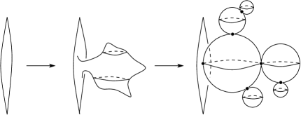
Figure 1: Bubbling of spheres.

illustrates the geometric picture behind that phenomenon. Bubbling is some kind of breaking phenomenon but the components here are discs and spheres. We do not need to take care of spheres bubbling off at all. Suppose that the boundary of the moduli space associated to the homotopy class $\phi$ we have breaking into a disc $\phi_{1}$ and a sphere $S_{1}$, i.e. $\phi=\phi_{1}*S_{1}$. Recall that the spheres in the symmetric product are generated by $S$, described in §2.2. Thus, $\phi=\phi_{1}*k\cdot S$ where $n_{z}(S)=1$. In consequence $n_{z}(\phi)$ is non-zero, contradicting the assumptions.

Definition 2.24.

For a point $x\in\mathbb{T}_{\alpha}\cap\mathbb{T}_{\beta}$ an $\alpha$-degenerate disc is a holomorphic disc $\phi\colon\thinspace[0,\infty)\times\mathbb{R}\longrightarrow\mbox{\rm Sym}^{g}(\Sigma)$ with the following boundary conditions $\phi(\{0\}\times\mathbb{R})\subset\mathbb{T}_{\alpha}$ and $\phi(p)\to x$ as $x\to\infty$.

Given a degenerate disc $\psi$, the associated domain $\mathcal{D}(\psi)$ equals a sphere with holes, i.e. $\mathcal{D}(\psi)$ equals a surface in $\Sigma$ with boundary the $\alpha$-curves. Since the $\alpha$-curves do not disconnect $\Sigma$, the domain covers the whole surface. Thus, $n_{z}(\psi)$ is non-zero, showing that degenerations are ruled out by assuming that $n_{z}=0$.

Proof of Theorem 2.4 with $\mathbb{Z}_{2}$-coefficients.

Fix an intersection $x\in\mathbb{T}_{\alpha}\cap\mathbb{T}_{\beta}$. We compute

$$\widehat{\partial}_{z}x = \widehat{\partial}_{z}\bigl{(}\sum_{y\in\mathbb{T}_{\alpha}\cap\mathbb{T}_{\beta}}\#\widehat{\mathcal{M}}(x,y)_{n_{z}=0}^{0}\cdot y\bigr{)}$$

$$= \sum_{y,w\in\mathbb{T}_{\alpha}\cap\mathbb{T}_{\beta}}\#\widehat{\mathcal{M}}(x,y)_{n_{z}=0}^{0}\#\widehat{\mathcal{M}}(y,w)_{n_{z}=0}^{0}\cdot w.$$

We have to show that the coefficient in front of $w$, denoted by $c(x,w)$ vanishes. Observe that the coefficient precisely equals the number of components (mod $2$) in

$$\widehat{\mathcal{M}}(x,y)_{n_{z}=0}^{0}\times\widehat{\mathcal{M}}(y,w)_{n_{z}=0}^{0}$$

Gluing gives an injection

$$\widehat{\mathcal{M}}(x,y)_{n_{z}=0}^{0}\times\widehat{\mathcal{M}}(y,w)_{n_{z}=0}^{0}\hookrightarrow\partial\widehat{\mathcal{M}}(x,w)_{n_{z}=0}^{1}.$$

By the compactification theorem the gluing map is a bijection, since bubbling and degenerations do not appear due to the condition $n_{z}=0$. Thus, (mod $2$) we have

$$c(x,w) = \#(\widehat{\mathcal{M}}(x,y)_{n_{z}=0}^{0}\times\widehat{\mathcal{M}}(y,w)_{n_{z}=0}^{0})$$

$$= \partial\widehat{\mathcal{M}}(x,w)_{n_{z}=0}^{1}$$

$$= 0,$$

which shows the theorem. ∎

Obviously, the proof breaks down in $\mathbb{Z}$-coefficients. We need the mod $2$ count of ends. There is a way to fix the proof. The goal is to make the map

$$f_{\mbox{\rm{\tiny glue}}}\colon\thinspace\mathcal{M}_{\phi_{2}}\times\mathcal{M}_{\phi_{1}}\hookrightarrow\partial\mathcal{M}_{\phi_{2}*\phi_{1}}$$

orientation preserving. For this to make sense we need the moduli spaces to be oriented. An orientation is given by choosing a section of the determinant line bundle over the moduli spaces. The determinant line bundle is defined as the bundle $\det([\phi])\longrightarrow\mathcal{M}_{\phi}$ given by putting together the spaces

$$\det(\psi)=\bigwedge\,\!\!\!^{\mbox{\rm\tiny max}}\ker(D_{\psi}\partial_{\mathcal{J}_{s}})\otimes\bigwedge\,\!\!\!^{\mbox{\rm\tiny max}}\ker((D_{\psi}\partial_{\mathcal{J}_{s}})^{*}),$$

where $\psi$ is an element of $\mathcal{M}_{\phi}$. If we achieve transversality for $\partial_{\mathcal{J}_{s}}$, i.e. it has transverse intersection with the zero section $\mathcal{B}_{0}\hookrightarrow\mathcal{L}$ then

$$\begin{array}[]{rcccc}\det(\psi)&=&\bigwedge\,\!\!\!^{\mbox{\rm\tiny max}}\ker(D_{\psi}\partial_{\mathcal{J}_{s}})&\otimes&\mathbb{R}^{*}\\ &=&\bigwedge\,\!\!\!^{\mbox{\rm\tiny max}}T_{\psi}\mathcal{M}_{\phi}&\otimes&\mathbb{R}^{*}.\end{array}$$

Thus, a section of the determinant line bundle defines an orientation of $\mathcal{M}_{\phi}$. These have to be chosen in a coherent fashion to make $f_{\mbox{\rm{\tiny glue}}}$ orientation preserving. The gluing construction gives a natural identification

$$\det(\phi_{1})\wedge\det(\phi_{2})\overset{\cong}{\longrightarrow}\det(\phi_{2}\#_{t}\phi_{1}).$$

Since these are all line bundles, this identification makes it possible to identify sections of $\det([\phi_{1}])\wedge\det([\phi_{2}])$ with sections of $\det([\phi_{2}*\phi_{1}])$. With this isomorphism at hand we are able to define a coherence condition. Namely, let $\mathnormal{o}(\phi_{1})$ and $\mathnormal{o}(\phi_{2})$ be sections of the determinant line bundles of the associated moduli spaces, then we need that under the identification given above we have

$$\mathnormal{o}(\phi_{1})\wedge\mathnormal{o}(\phi_{2})=\mathnormal{o}(\phi_{2}*\phi_{1}).$$ (2.10)

In consequence, a coherent system of orientations is a section $\mathnormal{o}(\phi)$ of the determinant line bundle $\det(\phi)$ for each homotopy class of Whitney discs $\phi$ connecting two intersection points such that equation (2.10) holds for each pair for which concatenation makes sense. It is not clear if these systems exist in general. By construction with respect to these coherent systems of orientations the map $f_{\mbox{\rm{\tiny glue}}}$ is orientation preserving.
In the case of Heegaard Floer theory there is an easy way giving a construction for coherent systems of orientations. Namely, fix a $\mbox{\rm Spin}^{c}$-structure $s$ and let $\{x_{0},\dots,x_{l}\}$ be the points representing $s$, i.e. $(s_{z})^{-1}(s)=\{x_{0},\dots,x_{l}\}$. Let $\phi_{1},\dots,\phi_{q}$ be a set of periodic classes in $\pi_{2}(x_{0},x_{0})$ representing a basis for $H^{1}(Y;\mathbb{Z})$, denote by $\theta_{i}$ an element of $\pi_{2}(x_{0},x_{i})$. A coherent system of orientations is constructed by choosing sections over all chosen discs, i.e. $\mathnormal{o}(\phi_{i})$, $i=1,\dots,q$ and $\mathnormal{o}(\theta_{j})$, $j=1,\dots,l$. Namely, for each homotopy class $\phi\in\pi_{2}(x_{i},x_{j})$ we have a presentation (cf. Lemma 2.8, Lemma 2.9 and (2.4))

$$\phi=a_{1}\phi_{1}+\dots+a_{q}\phi_{q}+\theta_{j}-\theta_{i}$$

inducing an orientation $\mathnormal{o}(\phi)$. This definition clearly defines a coherent system.
To give a proof of Theorem 2.4 in case of $\mathbb{Z}$-coefficients we have to translate orientations on the $0$-dimensional components of the moduli spaces $\widehat{\mathcal{M}}_{J_{s}}(x,y)$ of connecting Whitney discs into signs. For $\phi$ with $\mu(\phi)=1$ the translation action naturally induces an orientation on $\mathcal{M}_{\phi}$. Comparing this orientation with the coherent orientation induces a sign. We define the signed count as the count of the elements by taking into account the signs induced by the comparison of the action orientation with the coherent orientation.

Proof of Theorem 2.4 for $\mathbb{Z}$-coefficients.

We stay in the notation of the earlier proof. With the coherent system of orientations introduced we made the map

$$f_{\mbox{\rm{\tiny glue}}}\colon\thinspace\widehat{\mathcal{M}}(x,y)_{n_{z}=0}^{0}\times\widehat{\mathcal{M}}(y,w)_{n_{z}=0}^{0}\hookrightarrow\partial\widehat{\mathcal{M}}(x,z)_{n_{z}=0}^{1}$$

orientation preserving. Hence, we see that $c(x,w)$ equals

$$\#(\widehat{\mathcal{M}}(x,y)_{n_{z}=0}^{0}\times\widehat{\mathcal{M}}(y,w)_{n_{z}=0}^{0})$$

which in turn equals the oriented count of boundary components of $\partial\widehat{\mathcal{M}}(x,z)_{n_{z}=0}^{1}$. Since the space is $1$-dimensional, this count vanishes. ∎

2.3.1 More General Theories

There are variants of Heegaard Floer homology which do not force the condition $n_{z}=0$. To make the compactification work in that case we have to take care of boundary degenerations and spheres bubbling off. Both can be shown to be controlled in the sense that the proof of Theorem 2.4 for the general theories works the same way with some slight additions due to bubbling and degenerations. This article mainly focuses on the $\widehat{\mbox{\rm HF}}$-theory, so we exclude these matters from our exposition. Note just that we get rid of bubbling by a proper choice of almost complex structure. By choosing $j$ on $\Sigma$ appropriately there is a contractible open neighborhood of $sym^{g}(j)$ in $\mathcal{J}(j,\eta,V)$ for which all spheres miss the intersections $\mathbb{T}_{\alpha}\cap\mathbb{T}_{\beta}$. Moreover, for a generic choice of path $(\mathcal{J}_{s})_{s\in[0,1]}$ inside this neighborhood the signed count of degenerate discs is zero. With this information it is easy to modify the given proof for the general theories. We leave this to the interested reader or point him to [17].

2.4 Choice of Almost Complex Structure

Let $\Sigma$ be endowed with a complex structure $j$ and let $U\subset\Sigma$ be a subset diffeomorphic to a disc.

Theorem 2.25 (Riemann mapping theorem).

There is a $3$-dimensional connected family of holomorphic identifications of $U$ with the unit disc $\mathbb{D}\subset\mathbb{C}$.

Consequently, suppose that all moduli spaces are compact manifolds for the path $(\mathcal{J}_{s})_{s\in[0,1]}=sym^{g}(j)$. In this case we conclude from the Riemann mapping theorem the following corollary.

Corollary 2.26.

Let $\phi\colon\thinspace\mathbb{D}^{2}\longrightarrow\mbox{\rm Sym}^{g}(\Sigma)$ be a holomorphic disc with $\mathcal{D}(\phi)$ isomorphic to a disc. Then the moduli space $\widehat{\mathcal{M}}_{\phi}$ contains a unique element.

There are several ways to achieve this special situation. We call a domain $\mathcal{D}(\phi)$ $\alpha$-injective if all its multiplicities are $0$ or $1$ and its interior is disjoint from the $\alpha$-circles. We then say that the homotopy class $\phi$ is $\alpha$-injective.

Theorem 2.27.

Let $\phi\in\pi_{2}(x,y)$ be an $\alpha$-injective homotopy class and $j$ a complex structure on $\Sigma$. For generic perturbations of the $\alpha$-curves the moduli space $\mathcal{M}_{sym^{g}(j),\phi}$ is a smooth manifold.

In explicit calculations it will be nice to have all homotopy classes carrying holomorphic representatives to be $\alpha$-injective. In this case we can choose the path of almost complex structures in such a way that homotopy classes of Whitney discs with disc-shaped domains just admits a unique element. This is exactly what can be achieved in general to make the $\widehat{\mbox{\rm HF}}$-theory combinatorial. For a class of Heegaard diagrams called nice diagrams all moduli spaces with $\mu=1$ just admit one single element. In addition we have a precise description of how these domains look like. In $\mathbb{Z}_{2}$-coefficients with nice diagrams this results in a method of calculating the differential $\widehat{\partial}_{z}$ by counting the number of domains that fit into the scheme. This is successfully done for instance for the $\widehat{\mbox{\rm HF}}$-theory in [27].

Definition 2.28 (see [27]).

A pointed Heegaard diagram $(\Sigma,\alpha,\beta,z)$ is called nice if any region not containing $z$ is either a bigon or a square.

Definition 2.29 (see [27]).

A homotopy class is called an empty embedded $2n$-gon if it is topologically an embedded disc with $2n$ vertices at its boundary, it does not contain any $x_{i}$ or $y_{i}$ in its interior, and for each vertex $v$ the average of the coefficients of the four regions around $v$ is $1/4$.

For a nice Heegaard diagram one can show that all homotopy classes $\phi\in H(x,y,1)$ with $\mu(\phi)=1$ that admit holomorphic representatives are empty embedded bigons or empty embedded squares. Furthermore, for a generic choice of $j$ on $\Sigma$ the moduli spaces are regular under a generic perturbation of the $\alpha$-curves and $\beta$-curves. The moduli space $\widehat{\mathcal{M}}_{\phi}$ contains one single element. Thus, the theory can be computed combinatorially. We note the following property.

Theorem 2.30 (see [27]).

Every $3$-manifold admits a nice Heegaard diagram.

2.5 Dependence on the Choice of Orientation Systems

From their definition it is easy to reorder the orientation systems into equivalence classes. The elements in these classes give rise to isomorphic homologies. Let $\mathnormal{o}$ and $\mathnormal{o}^{\prime}$ be two orientation systems. We measure their difference

$$\delta\colon\thinspace H^{1}(Y;\mathbb{Z})\longrightarrow\mathbb{Z}_{2}$$

by saying that, given a periodic class $\phi\in\pi_{2}(x,x)$, we define $\delta(\phi)=0$ if $\mathnormal{o}(\phi)$ and $\mathnormal{o}^{\prime}(\phi)$ coincide, i.e. define equivalent sections, and $\delta(\phi)=1$, if $\mathnormal{o}(\phi)$ and $\mathnormal{o}^{\prime}(\phi)$ define non-equivalent sections. Thus, two systems are equivalent if $\delta=0$. Obviously, there are $2^{b_{1}(Y)}$ different equivalence classes of orientation systems. In general the Heegaard Floer homologies will depend on choices of equivalence classes of orientation systems. As an illustration we will discuss an example.

Example 2.2.

The manifold $\mathbb{S}^{2}\times\mathbb{S}^{1}$ admits a Heegaard splitting of genus one, namely $(T^{2},\alpha,\beta,z)$ where $\alpha$ and $\beta$ are two distinct meridians of $T^{2}$.
Unfortunately this is not an admissible diagram. By the universal coefficient theorem

$$H^{2}(\mathbb{S}^{2}\times\mathbb{S}^{1};\mathbb{Z})\cong Hom(H_{2}(\mathbb{S}^{2}\times\mathbb{S}^{1};\mathbb{Z}),\mathbb{Z})\cong Hom(\mathbb{Z},\mathbb{Z}).$$

Hence we can interpret $\mbox{\rm Spin}^{c}$-structures as homomorphisms $\mathbb{Z}\longrightarrow\mathbb{Z}$. For a number $q\in\mathbb{Z}$ define $s_{q}$ to be the $\mbox{\rm Spin}^{c}$-structure whose associated characteristic class, which we also call $s_{q}$, is given by $s_{q}(1)=q$. The two curves $\alpha$ and $\beta$ cut the torus into two components, where $z$ is placed in one of them. Denote the other component with $\mathcal{D}$. It is easy to see that the homology class $\mathcal{H}(\mathcal{D})$ is a generator of $H_{2}(\mathbb{S}^{2}\times\mathbb{S}^{1};\mathbb{Z})$. Thus, we have

$$\left<c_{1}(s_{q}),\mathcal{H}(\lambda\cdot\mathcal{D})\right>=\left<2\cdot s_{q},\mathcal{H}(\lambda\cdot\mathcal{D})\right>=2\cdot s_{q}(\lambda\cdot 1)=2\lambda q.$$

This clearly contradicts the weak admissibility condition. We fix this problem by perturbing the $\beta$-curve slightly to give a Heegaard diagram as illustrated in Figure 2.

2pt $\alpha$ [l] at 279 334 $x$ [Bl] at 283 244 $z$ [l] at 422 219 $\mathcal{D}_{1}$ [l] at 302 183 $\mathcal{D}_{2}$ [l] at 200 310 $y$ [tl] at 284 121 $\beta$ [r] at 146 44

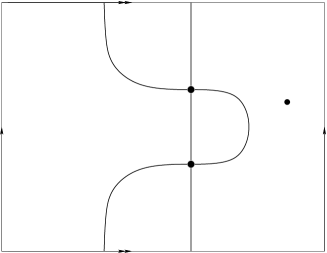
Figure 2: An admissible Heegaard diagram for $\mathbb{S}^{2}\times\mathbb{S}^{1}$.

By boundary orientations $\mathbb{Z}\left<(\mathcal{D}_{1}-\mathcal{D}_{2})\right>$ are all possible periodic domains.
Figure 2 shows that the chain module is generated by the points $x$ and $y$. A straightforward computation gives $\epsilon(x,y)=0$ (see §2.2 for a definition) and, hence, both intersections belong to the same $\mbox{\rm Spin}^{c}$-structure we will denote by $s_{0}$. Thus, the chain complex $\widehat{\mbox{\rm CF}}(\Sigma,\alpha,\beta;s_{0})$ equals $\mathbb{Z}\otimes\{x,y\}$. The regions $\mathcal{D}_{1}$ and $\mathcal{D}_{2}$ are both disc-shaped and hence $\alpha$-injective. Thus, the Riemann mapping theorem (see §2.4) gives

$$\#\widehat{\mathcal{M}}_{\phi_{1}}=1\;\;\mbox{\rm and }\#\widehat{\mathcal{M}}_{\phi_{2}}=1.$$

These two discs differ by the periodic domain generating $H^{1}(\mathbb{S}^{2}\times\mathbb{S}^{1};\mathbb{Z})$. Thus, we are free to choose the orientation on this generator (cf. §2.3). Hence, we may choose the signs on $\phi_{1}$ and $\phi_{2}$ arbitrarily. Thus, there are two equivalence classes of orientation systems. We define $\mathnormal{o}^{*}$ to be the system of orientations where the signs differ and $\mathnormal{o}_{0}$ where they are equal. Thus, we get two different homology theories

$$\widehat{\mbox{\rm HF}}(\mathbb{S}^{2}\times\mathbb{S}^{1},s_{0};\mathnormal{o}*) = \mathbb{Z}\oplus\mathbb{Z}$$

$$\widehat{\mbox{\rm HF}}(\mathbb{S}^{2}\times\mathbb{S}^{1},s_{0};\mathnormal{o}_{0}) = \mathbb{Z}_{2}.$$

However, there is a special choice of coherent orientation systems. We point the reader to §3 for a definition of $\mbox{\rm HF}^{\infty}$. Additionally, instead of using $\mathbb{Z}$-coefficients, we can use the ring $\mathbb{Z}[H_{1}(Y)]$ as coefficients for defining this Heegaard Floer group. The resulting group is denoted by $\underline{\mbox{\rm{HF}}}^{\infty}$. We point the reader to [17] for a precise definition. As a matter or completeness we cite:

Theorem 2.31 (see [18], Theorem 10.12).

Let $Y$ be a closed oriented $3$-manifold. Then there is a unique equivalence class of orientation system such that for each torsion $\mbox{\rm Spin}^{c}$-structure $s_{0}$ there is an isomorphism

$$\underline{\mbox{\rm{HF}}}^{\infty}(Y,s_{0})\cong\mathbb{Z}[U,U^{-1}]$$

as $\mathbb{Z}[U,U^{-1}]\otimes_{\mathbb{Z}}\mathbb{Z}[H^{1}(Y;\mathbb{Z})]$-modules.

3 The Homologies $\mbox{\rm HF}^{\infty}$, $\mbox{\rm HF}^{+}$, $\mbox{\rm HF}^{-}$

Given a pointed Heegaard diagram $(\Sigma,\alpha,\beta,z)$, we define $\mbox{\rm CF}^{-}(\Sigma,\alpha,\beta,z;s)$ as the free $\mathbb{Z}[U^{-1}]$-module generated by the points of intersection $(s_{z})^{-1}(s)\subset\mathbb{T}_{\alpha}\cap\mathbb{T}_{\beta}$. For an intersection $x$ we define

$$\partial^{-}x=\sum_{y\in(s_{z})^{-1}(s)}\sum_{\phi\in\mu^{-1}(1)}\#\widehat{\mathcal{M}}_{\phi}\cdot U^{-n_{z}(\phi)}y,$$

where $\mu^{-1}(1)$ are the homotopy classes in $\pi_{2}(x,y)$ with expected dimension equal to one. Note that in this theory we do not restrict to classes with $n_{z}=0$. This means even with weak admissibility imposed on the Heegaard diagram the proof of well-definedness as it was done in §2 breaks down.

Definition 3.1.

A Heegaard diagram $(\Sigma,\alpha,\beta,z)$ is called strongly admissible for the $\mbox{\rm Spin}^{c}$-structure $s$ if for every non-trivial periodic domain $\mathcal{D}$ such that $\left<c_{1}(s),H(\mathcal{D})\right>=2n\geq 0$ the domain $\mathcal{D}$ has some coefficient greater than $n$.

Imposing strong admissibility on the Heegaard diagram we can prove well-definedness by showing that only finitely many homotopy classes of Whitney discs contribute to the moduli space $\mathcal{M}_{\mathcal{J}_{s}}(x,y)$ (cf. §2).

Theorem 3.2.

The map $\partial^{-}$ is a differential.

As mentioned in §2, in this more general case we have to take a look at bubbling and degenerate discs. The proof follows the same lines as the proof of Theorem 2.4. With the remarks made in §2 it is easy to modify the given proof to a proof of Theorem 3.2 (see [17]). We define

$$\mbox{\rm CF}^{\infty}(\Sigma,\alpha,\beta;s)=\mbox{\rm CF}^{-}(\Sigma,\alpha,\beta;s)\otimes_{\mathbb{Z}[U^{-1}]}\mathbb{Z}[U,U^{-1}]$$

and denote by $\partial^{\infty}$ the induced differential. From the definition we get an inclusion of $\mbox{\rm CF}^{-}\hookrightarrow\mbox{\rm CF}^{\infty}$ whose cokernel is defined as $\mbox{\rm CF}^{+}(\Sigma,\alpha,\beta,s)$. Finally we get back to $\widehat{\mbox{\rm CF}}$ by

$$\widehat{\mbox{\rm CF}}(\Sigma,\alpha,\beta;s)=\frac{U\cdot\mbox{\rm CF}^{-}(\Sigma,\alpha,\beta;s)}{\mbox{\rm CF}^{-}(\Sigma,\alpha,\beta;s)}.$$

The associated homology theories are denoted by $\mbox{\rm HF}^{\infty}$, $\mbox{\rm HF}^{-}$ and $\widehat{\mbox{\rm HF}}$. There are two long exact sequences which can be derived easily from the definition of the Heegaard Floer homologies. To give an intuitive picture look at the following illustration:

$$\begin{array}[]{lcccccccccc}\mbox{\rm CF}^{\infty}&=&\dots&U^{-3}&U^{-2}&U^{-1}&U^{0}&U^{1}&U^{2}&U^{3}&\dots\\ \mbox{\rm CF}^{-}&=&\dots&U^{-3}&U^{-2}&U^{-1}&&&&&\\ \widehat{\mbox{\rm CF}}&=&&&&&U^{0}&&&&\\ \mbox{\rm CF}^{+}&=&&&&&U^{0}&U^{1}&U^{2}&U^{3}&\dots\end{array}$$

We see why the condition of weak admissibility is not strong enough to give a well-defined differential on $\mbox{\rm CF}^{\infty}$ or $\mbox{\rm CF}^{-}$. However, weak admissibility is enough to make the differential on $\mbox{\rm CF}^{+}$ well-defined, since the complex is bounded from below with respect to the obvious filtration given by the $U$-variable.

Lemma 3.3.

There are two long exact sequences where $s$ is a $\mbox{\rm Spin}^{c}$-structure of $Y$.

The explicit description illustrated above can be derived directly from the definition of the complexes. We leave this to the interested reader (see also [17]).

4 Topological Invariance

Given two Heegaard diagrams $(\Sigma,\alpha,\beta)$ and $(\Sigma^{\prime},\alpha^{\prime},\beta^{\prime})$ of a manifold $Y$, they are equivalent after a finite sequence of isotopies of the attaching circles, handle slides of the $\alpha$-curves and $\beta$-curves and stabilizations/destabilizations. Two Heegaard diagrams are equivalent if there is a diffeomorphism of the Heegaard surface interchanging the attaching circles. Obviously, equivalent Heegaard diagrams define isomorphic Heegaard Floer theories. To show that Heegaard Floer theory is a topological invariant of the manifold $Y$ we have to see that each of the moves, i.e. isotopies, handle slides and stabilization/destabilizations yield isomorphic theories. We will briefly sketch the topological invariance. This has two reasons: First of all the invariance proof uses ideas that are standard in Floer homology theories and hence appear frequently. The ideas provided from the invariance proof happen to be the standard techniques for proving exactness of sequences, proving invariance properties, and proving the existence of morphisms between Floer homologies. Thus, knowing the invariance proof, at least at the level of ideas, is crucial for an understanding of most of the papers published in this field. We will deal with the $\widehat{\mbox{\rm HF}}$-case and and point the reader to [17] for a general treatment.
The invariance proof contains several steps. We start showing invariance under the choice of path of admissible almost complex structures. Isotopies of the attaching circles are split up into two separate classes: Isotopies that generate/cancel intersection points and those which do not change the chain module. The invariance under the latter Heegaard moves immediately follows from the independence of the choice of almost complex structures. Such an isotopy is carried by an ambient isotopy inducing an isotopy of the symmetric product. We perturb the almost complex structure and thus interpret the isotopy as a perturbation of the almost complex structure. The former Heegaard moves have to be dealt with separately. We mimic the generation/cancellation of intersection points with a Hamiltonian isotopy and with it explicitly construct an isomorphism of the respective homologies by counting discs with dynamic boundary conditions. Stabilizations/ destabilizations is the easiest part to deal with: it follows from the behavior of the Heegaard Floer theory under connected sums. Finally, handle slide invariance will require us to define what can be regarded as the Heegaard Floer homological version of the pair-of-pants product in Floer homologies. This product has two nice applications. The first is the invariance under handle slides and the second is the association of maps to cobordisms giving the theory the structure of a topological field theory.

4.1 Stabilizations/Destabilizations

We determine the groups $\widehat{\mbox{\rm HF}}(\mathbb{S}^{2}\times\mathbb{S}^{1}\#\mathbb{S}^{2}\times\mathbb{S}^{1})$ as a model calculation for how the groups behave under connected sums.

2pt $z$ [l] at 240 141 $x_{1}$ [l] at 94 116 $y_{1}$ [l] at 385 120 $x_{2}$ [l] at 89 74 $y_{2}$ [l] at 380 74 $\mathcal{D}_{1}$ [t] at 161 26 $\mathcal{D}_{2}$ [l] at 105 10 $\mathcal{D}_{3}$ [tr] at 265 68 $\mathcal{D}_{4}$ [r] at 320 12

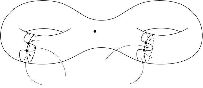
Figure 3: An admissible Heegaard diagram for $\mathbb{S}^{2}\times\mathbb{S}^{1}\#\mathbb{S}^{2}\times\mathbb{S}^{1}$.

Example 4.1.

We fix admissible Heegaard diagrams $(T^{2}_{i},\alpha_{i},\beta_{i})$ $i=1,2$ for $\mathbb{S}^{2}\times\mathbb{S}^{1}$ as in Example 2.2. To perform the connected sum of $\mathbb{S}^{2}\times\mathbb{S}^{1}$ with itself we choose $3$-balls such that their intersection $D$ with the Heegaard surface fulfills the property

$$\left.\mathcal{J}_{s}^{i}\right|_{D}=\mbox{\rm sym}(j_{i}).$$

Figure 3 pictures the Heegaard diagram we get for the connected sum. Denote by $T$ a small connected sum tube inside $\Sigma=T^{2}_{1}\#T^{2}_{2}$. By construction the induced almost complex structure equals

$$\left.(\mathcal{J}^{1}\#\mathcal{J}^{2})_{s}\right|_{T\times\Sigma}=sym^{2}(j^{1}\#j^{2}).$$

All intersection points belong to the same $\mbox{\rm Spin}^{c}$-structure $s_{0}$. For suitable $\mbox{\rm Spin}^{c}$-structures $s_{1}$, $s_{2}$ on $\mathbb{S}^{2}\times\mathbb{S}^{1}$ we have that $s_{0}=s_{1}\#s_{2}$ and

$$\widehat{\mbox{\rm CF}}(\Sigma,\alpha,\beta,s_{1}\#s_{2})=\mathbb{Z}\otimes\{(x_{i},y_{j})\,|\,i,j\in\{1,2\}\}\cong\widehat{\mbox{\rm CF}}(T^{2}_{1},s_{1})\otimes\widehat{\mbox{\rm CF}}(T^{2}_{2},s_{2}).$$

The condition $n_{z}=0$ implies that for every holomorphic disc $\phi\colon\thinspace\mathbb{D}^{2}\longrightarrow\mbox{\rm Sym}^{g}(\Sigma)$ the low-dimensional model (cf. §2) $\widehat{\phi}\colon\thinspace\widehat{\mathbb{D}}\longrightarrow\Sigma$ stays away from the tube $T$. Consequently we can split up $\widehat{\mathbb{D}}$ into

$$\widehat{\mathbb{D}}=\widehat{\mathbb{D}}_{1}\sqcup\widehat{\mathbb{D}}_{2},$$

where $\widehat{\mathbb{D}}_{i}$ are the components containing the preimage $(\widehat{\phi})^{-1}(T^{2}_{i}\backslash D)$. Restriction to these components determines maps $\widehat{\phi}_{i}\colon\thinspace\widehat{\mathbb{D}}_{i}\longrightarrow T^{2}_{i}$ inducing Whitney discs $\phi_{i}$ in the symmetric product $\mbox{\rm Sym}^{1}(T^{2})$. Thus, the moduli spaces split:

$$\begin{array}[]{rcl}\mathcal{M}_{(\mathcal{J}^{1}\#\mathcal{J}^{2})_{s}}((x_{i},y_{k}),(x_{j},y_{l}))_{n_{z}=0}&\overset{\cong}{\longrightarrow}&\mathcal{M}_{\mathcal{J}_{s}^{1}}(x_{i},x_{j})_{n_{z}=0}\times\mathcal{M}_{\mathcal{J}_{s}^{2}}(y_{k},y_{l})_{n_{z}=0}\\ \phi&\longmapsto&(\phi_{1},\phi_{2}).\end{array}$$

For moduli spaces with expected dimension $\mu=1$, a dimension count forces one of the factors to be constant. So, the differential splits, too, i.e. for $a_{i}\in\widehat{\mbox{\rm CF}}(T^{2}_{i},s_{i})$, $i=1,2$ we see that

$$\widehat{\partial}_{(\mathcal{J}^{1}\#\mathcal{J}^{2})_{s}}(a_{1}\otimes a_{2})=\widehat{\partial}_{\mathcal{J}_{s}^{1}}(a_{1})\otimes a_{2}+a_{1}\otimes\widehat{\partial}_{\mathcal{J}_{s}^{2}}(a_{2}).$$

And consequently

$$\widehat{\mbox{\rm HF}}(\mathbb{S}^{2}\times\mathbb{S}^{1}\#\mathbb{S}^{2}\times\mathbb{S}^{1},s_{1}\#s_{2};\mathnormal{o}_{1}\wedge\mathnormal{o}_{2})\cong\widehat{\mbox{\rm HF}}(\mathbb{S}^{2}\times\mathbb{S}^{1},s_{1};\mathnormal{o}_{1})\otimes\widehat{\mbox{\rm HF}}(\mathbb{S}^{2}\times\mathbb{S}^{1},s_{2};\mathnormal{o}_{2}).$$

The same line of arguments shows the general statement.

Theorem 4.1 (see [18]).

For closed, oriented $3$-manifolds $Y_{i}$, $i=1,2$ the Heegaard Floer homology of the connected sum $Y_{1}\#Y_{2}$ equals the tensor product of the Heegaard Floer homologies of the factors, i.e.

$$\widehat{\mbox{\rm HF}}(Y_{1}\#Y_{2})=H_{*}(\widehat{\mbox{\rm CF}}(Y_{1})\otimes\widehat{\mbox{\rm CF}}(Y_{2})),$$

where the chain complex on the right carries the natural induced boundary.

Stabilizing a Heegaard diagram of $Y$ means, on the manifold level, to do a connected sum with $\mathbb{S}^{3}$. We know that $\widehat{\mbox{\rm HF}}(\mathbb{S}^{3})=\mathbb{Z}$. By the classification of finitely generated abelian groups and the behavior of the tensor product, invariance follows.

4.2 Independence of the Choice of Almost Complex Structures

Suppose we are given a $1$-dimensional family of paths of $(j,\eta,V)$-nearly symmetric almost complex structures $(\mathcal{J}_{s,t})$. Given a Whitney disc $\phi$, we define $\mathcal{M}_{\mathcal{J}_{s,t},\phi}$ as the moduli space of Whitney discs in the homotopy class of $\phi$ which satisfy the equation

$$\frac{\partial\phi}{\partial s}(s,t)+\mathcal{J}_{s,t}\bigl{(}\frac{\partial\phi}{\partial t}(s,t)\bigr{)}=0.$$

Observe that there is no free translation action on the moduli spaces as on the moduli spaces we focused on while discussing the differential $\widehat{\partial}_{z}$. We define a map $\widehat{\Phi}_{\mathcal{M}_{\mathcal{J}_{s,t}}}$ between the theories $(\widehat{\mbox{\rm CF}}(\Sigma,\alpha,\beta,z),\widehat{\partial}_{\mathcal{J}_{s,i}})$ for $i=0,1$ by defining for $x\in\mathbb{T}_{\alpha}\cap\mathbb{T}_{\beta}$

$$\widehat{\Phi}_{\mathcal{J}_{s,t}}(x)=\sum_{y\in\mathbb{T}_{\alpha}\cap\mathbb{T}_{\beta}}\sum_{\phi\in H(x,y,0)}\#\mathcal{M}_{\mathcal{J}_{s,t},\phi}\cdot y,$$

where $H(x,y,0)\subset\pi_{2}(x,y)$ are the homotopy classes with expected dimension $\mu=0$ and intersection number $n_{z}=0$. There is an energy bound for all holomorphic Whitney discs which is independent of the particular Whitney disc or its homotopy class (see [17]). Thus, the moduli spaces are Gromov-compact manifolds, i.e. can be compactified by adding solutions coming from broken discs, bubbling of spheres and boundary degenerations (cf. §2.3). Since we stuck to the $\widehat{\mbox{\rm HF}}$-theory we impose the condition $n_{z}=0$ which circumvents bubbling of spheres and boundary degenerations (see §2.3).
To check that $\widehat{\Phi}$ is a chain map, we compute

$$\widehat{\partial}_{J_{s,1}}\circ\widehat{\Phi}_{J_{s,t},z}(x)-\widehat{\Phi}_{J_{s,t}}\circ\widehat{\partial}_{J_{s,0},z}(x) = \sum_{\underset{\phi\in H(x,y,0),\psi\in H(y,z,1)}{y,z}}\#\mathcal{M}_{J_{s,t}}(\phi)\#\widehat{\mathcal{M}}_{J_{s,1}}(\psi)z\$$

$$-\sum_{\underset{\phi\in H(x,y,1),\psi\in H(y,z,0)}{y,z}}\#\widehat{\mathcal{M}}_{J_{s,0}}(\phi)\#\mathcal{M}_{J_{s,t}}(\psi)z$$

$$= \sum_{z}c(x,z)\cdot z.$$

The coefficient $c(x,z)$ is given by

$$\sum_{y,I}\bigl{(}\#\mathcal{M}_{\mathcal{J}_{s,t},\phi}\cdot\#\widehat{\mathcal{M}}_{\mathcal{J}_{s,1},\psi}-\#\widehat{\mathcal{M}}_{\mathcal{J}_{s,0},\widetilde{\psi}}\cdot\#\mathcal{M}_{\mathcal{J}_{s,t},\widetilde{\phi}}\bigr{)},$$ (4.1)

where $I$ consists of pairs

$$(\phi,\widetilde{\phi})\in H(x,y,0)\times H(y,z,0)\;\text{ and }(\psi,\widetilde{\psi})\in H(x,y,1)\times H(y,z,1).$$

Looking at the ends of the moduli spaces $\mathcal{M}_{J_{s,t}}(\eta)$ for an $\eta\in H(x,z,1)$, the gluing construction (cf. §2.3) together with the compactification argument mentioned earlier provides the following ends:

$$\Bigl{(}\bigsqcup_{\eta=\psi*\phi}(\mathcal{M}_{J_{s,t}}(\phi)\times\widehat{\mathcal{M}}_{J_{s,1}}(\psi))\Bigr{)}\sqcup\Bigl{(}\bigsqcup_{\eta=\widetilde{\psi}*\widetilde{\phi}}(\widehat{\mathcal{M}}_{J_{s,0}}(\widetilde{\psi})\times\mathcal{M}_{J_{s,t}}(\widetilde{\phi}))\Bigr{)},$$ (4.2)

where the expected dimensions of $\phi$ and $\widetilde{\phi}$ are $1$ and of $\psi$ and $\widetilde{\psi}$ they are $0$. A signed count of (4.2) precisely reproduces (4.1) and hence $c(x,z)=0$ – at least in $\mathbb{Z}_{2}$-coefficients. To make this work in general, i.e. with coherent orientations, observe that we have the following condition imposed on the sections:

$$\mathnormal{o}_{s,t}(\phi)\wedge\mathnormal{o}_{1}(\psi)=-\mathnormal{o}_{0}(\widetilde{\psi})\wedge\mathnormal{o}_{s,t}(\widetilde{\phi}).$$

We get an identification of orientation systems, $\xi$ say, such that $\Phi$ is a chain map between

$$(\widehat{\mbox{\rm CF}}(\Sigma,\alpha,\beta,z),\widehat{\partial}_{\mathcal{J}_{s,0}}^{\,\mathnormal{o}})\longrightarrow(\widehat{\mbox{\rm CF}}(\Sigma,\alpha,\beta,z),\widehat{\partial}_{\mathcal{J}_{s,1}}^{\,\xi(\mathnormal{o})}).$$

We reverse the direction of the isotopy and define a map $\widehat{\Phi}_{\mathcal{J}_{s,1-t}}$. The compositions

$$\widehat{\Phi}_{\mathcal{J}_{s,1-t}}\circ\widehat{\Phi}_{\mathcal{J}_{s,t}}\;\;\mbox{\rm and }\;\;\widehat{\Phi}_{\mathcal{J}_{s,t}}\circ\widehat{\Phi}_{\mathcal{J}_{s,1-t}}$$

are both chain homotopic to the identity. In the following we will discuss the chain homotopy equivalence for the map $\widehat{\Phi}_{\mathcal{J}_{s,t}}\circ\widehat{\Phi}_{\mathcal{J}_{s,1-t}}$.
Define a path $\mathcal{J}_{s,t}(\tau)$ such that $\mathcal{J}_{s,t}(0)=\mathcal{J}_{s,t}*\mathcal{J}_{s,1-t}$ and $\mathcal{J}_{s,t}(1)=\mathcal{J}_{s,0}$. The existence of this path follows from the fact that we choose the paths inside a contractible set (cf. §2.3 or see [17]). Define the moduli space

$$\mathcal{M}_{\mathcal{J}_{s,t}(\tau),\phi}=\bigcup_{\tau\in[0,1]}\mathcal{M}_{\mathcal{J}_{s,t}(\tau),\phi}.$$

Theorem 4.2.

Let $\mathcal{J}_{(t_{1},\dots,t_{n})}$ be an $n$-parameter family of generic almost complex structures and $\phi$ a homotopy class of Whitney discs with expected dimension $\mu(\phi)$. Then $\mathcal{M}$, defined as the union of $\mathcal{M}_{\mathcal{J}_{(t_{1},\dots,t_{n})},\phi}$ over all $\mathcal{J}_{(t_{1},\dots,t_{n})}$ in the family, is a manifold of dimension $\mu(\phi)+n$.

There are two types of boundary components: the one type of boundary component coming from variations of the Whitney disc $\phi$ which are breaking, bubbling or degenerations and the other type of ends coming from variations of the almost complex structure.
We define a map

$$\widehat{H}_{\mathcal{J}_{s,t}(\tau)}(x)=\sum_{y\in\mathbb{T}_{\alpha}\cap\mathbb{T}_{\beta}}\sum_{\phi\in H(x,y,-1)}\#\mathcal{M}_{\mathcal{J}_{s,t}(\tau),\phi}\cdot y,$$

where $H(x,y,-1)\subset\pi_{2}(x,y)$ are the homotopy classes $\phi$ with $n_{z}(\phi)=0$ and expected dimension $\mu(\phi)=-1$. According to Theorem 4.2, the manifold $\mathcal{M}_{\mathcal{J}_{s,t}(\tau),\phi}$ is $0$-dimensional. We claim that $\widehat{H}$ is a chain homotopy between $\widehat{\Phi}_{\mathcal{J}_{s,t}}\circ\widehat{\Phi}_{\mathcal{J}_{s,1-t}}$ and the identity. By definition, the equation

$$\widehat{\Phi}_{\mathcal{J}_{s,t}}\circ\widehat{\Phi}_{\mathcal{J}_{s,1-t}}-\mbox{\rm id}-(\widehat{\partial}_{\mathcal{J}_{s,0}}\circ\widehat{H}_{\mathcal{J}_{s,t}(\tau)}+\widehat{H}_{\mathcal{J}_{s,t}(\tau)}\circ\widehat{\partial}_{\mathcal{J}_{s,1}})=0$$ (4.3)

has to hold. Look at the ends of $\mathcal{M}_{\mathcal{J}_{s,t}(\tau)}(\psi)$ for $\mu(\psi)=0$. This is a $1$-dimensional space, and there are the ends

$$\Bigl{(}\bigsqcup_{\psi=\eta*\phi}\widehat{\mathcal{M}}_{\mathcal{J}_{s,0},\eta}\times\mathcal{M}_{\mathcal{J}_{s,t}(\tau),\phi}\Bigr{)}\sqcup\Bigl{(}\bigsqcup_{\psi=\widetilde{\eta}*\widetilde{\phi}}\mathcal{M}_{\mathcal{J}_{s,t}(\tau),\widetilde{\eta}}\times\widehat{\mathcal{M}}_{\mathcal{J}_{s,1},\widetilde{\phi}}\Bigr{)}$$

coming from variations of the Whitney disc, and the ends

$$\mathcal{M}_{\mathcal{J}_{s,t}(0),\psi}\sqcup\mathcal{M}_{\mathcal{J}_{s,t}(1),\psi}$$

coming from variations of the almost complex structure. These all together precisely produce the coefficients in equation (4.3). Thus, the Floer homology is independent of the choice of $(j,\eta,V)$-nearly symmetric path. Variations of $\eta$ and $V$ just change the contractible neighborhood $\mathcal{U}$ around $\xi_{sym}^{g}(j)$ containing the admissible almost complex structures. So, the theory is independent of these choices, too. A $j^{\prime}$-nearly symmetric path can be approximated by a $j$-symmetric path given that $j^{\prime}$ is close to $j$. The set of complex structures on a surface $\Sigma$ is connected, so step by step one can move from a $j$-symmetric path to any $j^{\prime}$-symmetric path.

4.3 Isotopy Invariance

Every isotopy of an attaching circle can be divided into two classes: creation/anhillation of pairs of intersection points and isotopies not affecting transversality. An isotopy of an $\alpha$-circle of the latter type induces an isotopy of $\mathbb{T}_{\alpha}$ in the symmetric product. Compactness of the $\mathbb{T}_{\alpha}$ tells us that there is an ambient isotopy $\phi_{t}$ carrying the isotopy. With this isotopy we perturb the admissible path of almost complex structures as

$$\widetilde{\mathcal{J}}_{s}=(\phi_{1}^{-1})_{*}\circ\mathcal{J}_{s}\circ(\phi_{1})_{*}$$

giving rise to a path of admissible almost complex structures. The diffeomorphism $\phi_{1}$ induces an identification of the chain modules. The moduli spaces defined by $\mathcal{J}_{s}$ and $\widetilde{\mathcal{J}}_{s}$ are isomorphic. Hence

$$H_{*}(\widehat{\mbox{\rm CF}}(\Sigma,\alpha,\beta),\widehat{\partial}_{z}^{\mathcal{J}_{s}})=H_{*}(\widehat{\mbox{\rm CF}}(\Sigma,\alpha^{\prime},\beta),\widehat{\partial}_{z}^{\widetilde{\mathcal{J}}_{s}})=H_{*}(\widehat{\mbox{\rm CF}}(\Sigma,\alpha^{\prime},\beta),\widehat{\partial}_{z}^{\mathcal{J}_{s}}),$$ (4.4)

where the last equality follows from the considerations in §4.2. This chain of equalities shows that the isotopies discussed can be interpreted as variations of the almost complex structure.
The creation/cancellation of pairs of intersection points is done with an exact Hamiltonian isotopy supported in a small neighborhood of two attaching circles. We cannot use the methods from §4.2 to create an isomorphism between the associated Floer homologies. At a certain point the isotopy violates transversality as the attaching tori do not intersect transversely. Thus, the arguments of §4.2 for the right equality in (4.4) break down.
Consider an exact Hamiltonian isotopy $\psi_{t}$ of an $\alpha$-curve generating a canceling pair of intersections with a $\beta$-curve. We will just sketch the approach used in this context, since the ideas are similar to the ideas introduced in §4.2.
Define $\pi_{2}^{t}(x,y)$ as the set of Whitney discs $\phi$ with dynamic boundary conditions in the following sense:

$$\phi(i) = x,$$

$$\phi(-i) = y,$$

$$\phi(0+it) \in \Psi_{t}(\mathbb{T}_{\alpha})$$

$$\phi(1+it) \subset \mathbb{T}_{\beta}$$

for all $t\in\mathbb{R}$. Spoken geometrically, we follow the isotopy with the $\alpha$-boundary of the Whitney disc. Correspondingly, we define the moduli spaces of $\mathcal{J}_{s}$-holomorphic Whitney discs with dynamic boundary conditions as $\mathcal{M}^{t}(x,y)$. For $x\in\mathbb{T}_{\alpha}\cap\mathbb{T}_{\beta}$ define

$$\widehat{\Gamma}_{\Psi_{t}}(x)=\sum_{y\in\mathbb{T}_{\alpha}\cap\mathbb{T}_{\beta}}\sum_{\phi\in H_{t}(x,y,0)}\#\mathcal{M}^{t}_{\mathcal{J}_{s},\phi}\cdot y,$$

where $H_{t}(x,y,0)\subset\pi_{2}^{t}(x,y)$ are the homotopy classes with expected dimension $\mu=0$ and $n_{z}=0$. Using the low-dimensional model introduced in §2, Ozváth and Szabó prove the following property.

Theorem 4.3 (see [17], §7.3).

There exists a $t$-independent energy bound for holomorphic Whitney discs independent of its homotopy class.

The existence of this energy bound shows that there are Gromov compactifications of the moduli spaces of Whitney discs with dynamic boundary conditions.

Theorem 4.4.

The map $\widehat{\Gamma}_{\Psi_{t}}$ is a chain map. Using the inverse isotopy we define $\widehat{\Gamma}_{\Psi_{1-t}}$ such that the compositions $\widehat{\Gamma}_{\Psi_{t}}\circ\widehat{\Gamma}_{\Psi_{1-t}}$ and $\widehat{\Gamma}_{\Psi_{1-t}}\circ\widehat{\Gamma}_{\Psi_{t}}$ are chain homotopic to the identity.

The proof follows the same lines as in §4.2. We leave the proof to the interested reader.

4.4 Handle slide Invariance

4.4.1 The Pair-of-Pants Product

In this paragraph we will introduce the Heegaard Floer incarnation of the pair-of-pants product and with it associate to cobordisms maps between the Floer homologies of their boundary components. In case the cobordisms are induced by handle slides the associated maps are isomorphisms on the level of homology. The maps we will introduce will count holomorphic triangles in the symmetric product with appropriate boundary conditions. We have to discuss well-definedness of the maps and that they are chain maps. To do that we have to follow similar lines as it was done for the differential. Because of the strong parallels we will shorten the discussion here. We strongly advise the reader to first read §2 before continuing.

Definition 4.5.

A set of data $(\Sigma,\alpha,\beta,\gamma)$, where $\Sigma$ is a surface of genus $g$ and $\alpha$, $\beta$, $\gamma$ three sets of attaching circles, is called a Heegaard triple diagram.

We denote the $3$-manifolds determined be taking pairs of these attaching circles as $Y_{\alpha\beta}$, $Y_{\beta\gamma}$ and $Y_{\alpha\gamma}$. We fix a point $z\in\Sigma\backslash\{\alpha\cup\beta\cup\gamma\}$ and define a product

$$\widehat{f}_{\alpha\beta\gamma}\colon\thinspace\widehat{\mbox{\rm CF}}(\Sigma,\alpha,\beta,z)\otimes\widehat{\mbox{\rm CF}}(\Sigma,\beta,\gamma,z)\longrightarrow\widehat{\mbox{\rm CF}}(\Sigma,\alpha,\gamma,z)$$

by counting holomorphic triangles with suitable boundary conditions: A Whitney triangle is a map $\phi\colon\thinspace\Delta\longrightarrow\mbox{\rm Sym}^{g}(\Sigma)$ with boundary conditions as illustrated in Figure 4. We call the respective boundary segments its $\alpha$-, $\beta$- and $\gamma$-boundary. The boundary points, as should be clear from the picture, are $x\in\mathbb{T}_{\alpha}\cap\mathbb{T}_{\beta}$, $w\in\mathbb{T}_{\alpha}\cap\mathbb{T}_{\gamma}$ and $y\in\mathbb{T}_{\beta}\cap\mathbb{T}_{\gamma}$. The set of homotopy classes of Whitney discs connecting $x$, $w$ and $y$ is denoted by $\pi_{2}(x,y,w)$.

2pt $w$ [tr] at 7 34 $x$ [B] at 126 235 $y$ [tl] at 247 27 $\mathbb{T}_{\alpha}$ [Br] at 71 136 $\mathbb{T}_{\beta}$ [Bl] at 191 136 $\mathbb{T}_{\gamma}$ [t] at 126 26

Figure 4: A Whitney triangle and its boundary conditions.

Denote by $\mathcal{M}^{\Delta}_{\phi}$ the moduli space of holomorphic triangles in the homotopy class of $\phi$. Analogous to the case of discs we denote by $\mu(\phi)$ its expected/formal dimension. For $x\in\mathbb{T}_{\alpha}\cap\mathbb{T}_{\beta}$ define

$$\widehat{f}_{\alpha\beta\gamma}(x\otimes y)=\sum_{w\in\mathbb{T}_{\alpha}\cap\mathbb{T}_{\gamma}}\sum_{\phi\in H(x,y,w,0)}\#\mathcal{M}^{\Delta}_{\phi}\cdot w,$$

where $H(x,y,w,0)\subset\pi_{2}(x,y,w)$ is the subset with $\mu=0$ and $n_{z}=0$. The set of homotopy classes of Whitney discs fits into an exact sequence

$$0\longrightarrow\pi_{2}(\mbox{\rm Sym}^{g}(\Sigma))\longrightarrow\pi_{2}(x,y,w)\longrightarrow\ker(n_{z})\longrightarrow 0,$$ (4.5)

where $n_{z}$ provides a splitting for the sequence. We define

$$X_{\alpha\beta\gamma}=\frac{(\Delta\times\Sigma)\cup e_{\alpha}\times U_{\alpha}\cup e_{\beta}\times U_{\beta}\cup e_{\gamma}\times U_{\gamma}}{(e_{\alpha}\times\Sigma)\sim(e_{\alpha}\times\partial U_{\alpha}),(e_{\beta}\times\Sigma)\sim(e_{\beta}\times\partial U_{\beta}),(e_{\gamma}\times\Sigma)\sim(e_{\gamma}\times\partial U_{\gamma})},$$

where $U_{\alpha}$, $U_{\beta}$ and $U_{\gamma}$ are the handlebodies determined by the $2-$handles associated to the attaching circles $\alpha$, $\beta$ and $\gamma$, and $e_{\alpha}$, $e_{\beta}$ and $e_{\gamma}$ are the edges of the triangle $\Delta$. The manifold $X_{\alpha\beta\gamma}$ is $4$-dimensional with boundary

$$\partial X_{\alpha\beta\gamma}=Y_{\alpha\beta}\sqcup Y_{\beta\gamma}\sqcup-Y_{\alpha\gamma}.$$

Lemma 4.6.

The kernel of $n_{z}$ equals $H_{2}(X_{\alpha\beta\gamma};\mathbb{Z})$

Combining (4.5) with Lemma 4.6 we get an exact sequence

$$0\longrightarrow\pi_{2}(\mbox{\rm Sym}^{g}(\Sigma))\longrightarrow\pi_{2}(x,y,w)\overset{\mathcal{H}}{\longrightarrow}H_{2}(X_{\alpha\beta\gamma};\mathbb{Z})\longrightarrow 0,$$ (4.6)

where $\mathcal{H}$ is defined similarly as for discs (cf. §2.2). Of course there is a low-dimensional model for triangles and the discussion we have done for discs carries over verbatim for triangles. The condition $n_{z}=0$ makes the product $f_{\alpha\beta\gamma}$ well-defined in case $H_{2}(X_{\alpha\beta\gamma};\mathbb{Z})$ is trivial. Analogous to our discussion for Whitney discs and the differential, we have to include a condition controlling the periodic triangles, i.e. the triangles associated to elements in $H_{2}(X_{\alpha\beta\gamma};\mathbb{Z})$. A domain $\mathcal{D}$ of a triangle is called triply-periodic if its boundary consists of a sum of $\alpha$-,$\beta$- and $\gamma$-curves such that $n_{z}=0$.

Definition 4.7.

A pointed triple diagram $(\Sigma,\alpha,\beta,\gamma,z)$ is called weakly admissible if all triply-periodic domains $\mathcal{D}$ which can be written as a sum of doubly-periodic domains have both positive and negative coefficients.

This condition is the natural transfer of weak-admissibility from discs to triangles. One can show that for given $j,k\in\mathbb{Z}$ there exist just a finite number of Whitney triangles $\phi\in\pi_{2}(x,y,w)$ with $\mu(\phi)=j$, $n_{z}(\phi)=k$ and $\mathcal{D}(\phi)\geq 0$.
For a given homotopy class $\psi\in\pi_{2}(x,y,w)$ with $\mu(\psi)=1$ we compute the ends by shrinking a properly embedded arc to a point (see the description of convergence in §2.3). There are three different ways to do this in a triangle. Each time we get a concatenation of a disc with a triangle. By boundary orientations we see that each of these boundary components contributes to one of the terms in the following sum

$$\widehat{f}_{\alpha\beta\gamma}\circ(\widehat{\partial}_{\alpha\beta}(x)\otimes y)+\widehat{f}_{\alpha\beta\gamma}\circ(x\otimes\widehat{\partial}_{\beta\gamma}(y))-\widehat{\partial}_{\alpha\gamma}\circ\widehat{f}_{\alpha\beta\gamma}(x\otimes y).$$ (4.7)

Conversely, the coefficient at any of these terms is given by a product of signed counts of moduli spaces of discs and moduli spaces of triangles and hence – by gluing – comes from one of these contributions. The sum in (4.7) vanishes, showing that $\widehat{f}_{\alpha\beta\gamma}$ descends to a pairing $\widehat{f}^{*}_{\alpha\beta\gamma}$ between the Floer homologies.

4.4.2 Holomorphic rectangles

Recall that the set of biholomorphisms of the unit disc is a $3$-dimensional connected family. If we additionally fix a point we decrease the dimension of that family by one. A better way to formulate this is to say that the set of biholomorphishms of the unit disc with one fixed point is a $2$-dimensional family. Fixing two further points reduces to a $0$-dimensional set. If we additionally fix a fourth point the rectangle together with these four points uniquely defines a conformal structure. Variation of the fourth point means a variation of the conformal structure. Indeed one can show that there is a uniformization of a holomorphic rectangle, i.e. a rectangle with fixed conformal structure, which we denote by $\square$,

$$\square\longrightarrow[0,l]\times[0,h],$$

where the ratio $l/h$ uniquely determines the conformal structure. With this uniformization we see that $\mathcal{M}(\square)\cong\mathbb{R}$. The uniformization is area-preserving and converging to one of the ends of $\mathcal{M}(\square)$ means to stretch the rectangle infinitely until it breaks at the end into a concatenation of two triangles.

Theorem 4.8.

Given another set of attaching circles $\delta$ defining a map $\widehat{f}_{\alpha\gamma\delta}$, the following equality holds:

$$\widehat{f}^{*}_{\alpha\beta\gamma}(\widehat{f}^{*}_{\alpha\gamma\delta}(\,\cdot\otimes\,\cdot)\otimes\,\cdot)-\widehat{f}^{*}_{\alpha\beta\delta}(\,\cdot\otimes\widehat{f}^{*}_{\beta\gamma\delta}(\,\cdot\otimes\,\cdot))=0.$$ (4.8)

This property is called associativity.

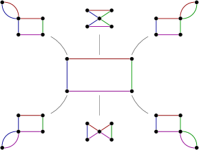
Figure 5: Ends of the moduli space of holomorphic rectangles.

If we count holomorphic Whitney rectangles with boundary conditions in $\alpha$, $\beta$, $\gamma$ and $\delta$ and with $\mu=1$ (see Definition 2.6) the ends of the associated moduli space will look like pictured in Figure 5. Note that we are talking about holomorphicity with respect to an arbitrary conformal structure on the rectangle. There will be two types of ends. We will have a degeneration into a concatenation of triangles by variation of the conformal structure on the rectangle and breaking into a concatenation of a rectangle with a disc by variation of the rectangle. By Figure 5 an appropriate count of holomorphic rectangles will be a natural candidate for a chain homotopy proving equation (4.8). Define a pairing

$$H\colon\thinspace\widehat{\mbox{\rm CF}}(\Sigma,\alpha,\beta,z)\otimes\widehat{\mbox{\rm CF}}(\Sigma,\beta,\gamma,z)\otimes\widehat{\mbox{\rm CF}}(\Sigma,\gamma,\delta,z)\longrightarrow\widehat{\mbox{\rm CF}}(\Sigma,\alpha,\delta,z)$$

by counting holomorphic Whitney rectangles with boundary components as indicated in Figure 6

2pt $\mathbb{T}_{\alpha}$ [r] at 10 65 $\mathbb{T}_{\beta}$ [B] at 79 110 $\mathbb{T}_{\gamma}$ [t] at 79 25 $\mathbb{T}_{\delta}$ [l] at 155 65

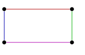
Figure 6: The boundary conditions of rectangles for the definition of $H$.

and $\mu=0$. By counting ends of the moduli space of holomorphic rectangles with $\mu=1$ we have six contributing ends. These ends are pictured in Figure 5. The four ends coming from breaking contribute to

$$\widehat{\partial}\circ H(\,\cdot\otimes\,\cdot\otimes\,\cdot)+H\circ\widehat{\partial}(\,\cdot\otimes\,\cdot\otimes\,\cdot).$$ (4.9)

In addition there are two ends coming from degenerations of the conformal structure on the rectangle. These give rise to

$$\widehat{f}_{\alpha\beta\gamma}(\widehat{f}_{\alpha\gamma\delta}(\,\cdot\otimes\,\cdot)\otimes\,\cdot)-\widehat{f}_{\alpha\beta\delta}(\,\cdot\otimes\widehat{f}_{\beta\gamma\delta}(\,\cdot\otimes\,\cdot)).$$ (4.10)

We see that the sum of (4.9) and (4.10) vanishes, showing that $H$ is a chain homotopy proving associativity.

4.4.3 Special Case – Handle Slides

Handle slides provide special Heegaard triple diagrams. Let $(\Sigma,\alpha,\beta,z)$ be an admissible pointed Heegaard diagram and define $(\Sigma,\alpha,\gamma,z)$ by handle sliding $\beta_{1}$ over $\beta_{2}$. We push the $\gamma_{i}$ off the $\beta_{i}$ to make them intersect transversely in two cancelling points. This defines a triple diagram, and obviously $Y_{\beta\gamma}$ equals the connected sum $\#^{g}(\mathbb{S}^{2}\times\mathbb{S}^{1})$.
A very important observation is that the Heegaard Floer groups of connected sums of $\mathbb{S}^{2}\times\mathbb{S}^{1}$ admit a top-dimensional generator. By Example 2.2 and Theorem 4.1,

$$\widehat{\mbox{\rm HF}}(\#^{g-1}(\mathbb{S}^{2}\times\mathbb{S}^{1}),\mathnormal{o}^{*})\cong\mathbb{Z}^{2g-2}\cong H_{*}(T^{g};\mathbb{Z}),$$

where the last identification is done using the $\bigwedge\,\!\!\!^{*}(H_{1}/Tor)$-module structure (see [17]). We claim that the behavior of the Heegaard Floer groups under connected sums can be carried over to the module structure, and thus it remains to show the assertion for the case $g=1$. But this is not hard to see.
Each pair $(\beta_{i},\gamma_{i})$ has two intersections $x^{+}_{i}$ and $x^{-}_{i}$. Which one is denoted how is determined by the following criterion: there is a disc-shaped domain connecting $x^{+}_{i}$ with $x^{-}_{i}$ with boundary in $\beta_{i}$ and $\gamma_{i}$. The point

$$x^{+}=\{x^{+}_{1},\dots,x^{+}_{g}\}$$

is a cycle whose associated homology class is the top-dimensional generator we denote by $\widehat{\Theta}_{\beta\gamma}$. For a detailed treatment of the top-dimensional generator we point the reader to [17].
Plugging in the generator we define a map

$$\widehat{F}_{\alpha\beta\gamma}=\widehat{f}^{*}_{\alpha\beta\gamma}(\,\cdot\otimes\widehat{\Theta}_{\beta\gamma})\colon\thinspace\widehat{\mbox{\rm HF}}(\Sigma,\alpha,\beta,z)\longrightarrow\widehat{\mbox{\rm HF}}(\Sigma,\alpha,\gamma,z)$$

between the associated Heegaard Floer groups. Our intention is to show that this is an isomorphism.
We can slide the $\gamma_{1}$ back over $\gamma_{2}$ to give another set of attaching circles we denote by $\delta$. Of course we make the curves intersecting all other sets of attaching circles transversely and introduce pairs of intersections points of the $\delta$-curves with the $\gamma$-and $\beta$-curves. Let $\widehat{F}_{\alpha\gamma\delta}$ be the associated map. Then the associativity given in (4.8) translates into

$$\widehat{f}^{*}_{\alpha\beta\gamma}(\widehat{f}^{*}_{\alpha\gamma\delta}(\,\cdot\otimes\widehat{\Theta}_{\gamma\delta})\otimes\widehat{\Theta}_{\beta\gamma})-\widehat{f}^{*}_{\alpha\beta\delta}(\,\cdot\otimes\widehat{f}^{*}_{\beta\gamma\delta}(\widehat{\Theta}_{\beta\gamma}\otimes\widehat{\Theta}_{\gamma\delta}))=0.$$

The proof of the following lemma will be done in detail. It is the first explicit calculation using the low-dimensional model in a non-trivial manner.

Lemma 4.9.

Given the map $\widehat{f}_{\alpha\gamma\delta}$, we have

$$\widehat{f}_{\beta\gamma\delta}(\widehat{\Theta}_{\beta\gamma}\otimes\widehat{\Theta}_{\gamma\delta})=\widehat{\Theta}_{\beta\delta}.$$

Hence, we have $\widehat{F}_{\beta\gamma\delta}(\widehat{\Theta}_{\beta\gamma})=\widehat{\Theta}_{\beta\delta}$.

Proof.

The complement of the $\beta$-circles in $\Sigma$ is a sphere with holes. We have a precise description of how the sets $\gamma$ and $\delta$ look like relative to $\beta$. The Heegaard surface cut open along the $\beta$-curves can be identified with a sphere with holes by using an appropriate diffeomorphism. Doing so, the diagram $(\Sigma,\beta,\gamma,\delta)$ will look like given in Figure 7. In

2pt $\widehat{\Theta}_{\gamma\delta}$ [l] at 198 383 $\widehat{\Theta}_{\beta\delta}$ [b] at 188 318 $\widehat{\Theta}_{\beta\gamma}$ [l] at 175 235 $\widehat{\Theta}^{-}_{\beta\delta}$ [r] at 500 285 $\mathcal{D}_{1}$ [tr] at 24 328 $\mathcal{D}_{2}$ [l] at 392 377 $\mathcal{D}_{3}$ [r] at 526 385 $z$ [l] at 469 214 $\gamma$ [b] at 193 158 $\delta$ [l] at 160 69 $\beta$ [br] at 122 67

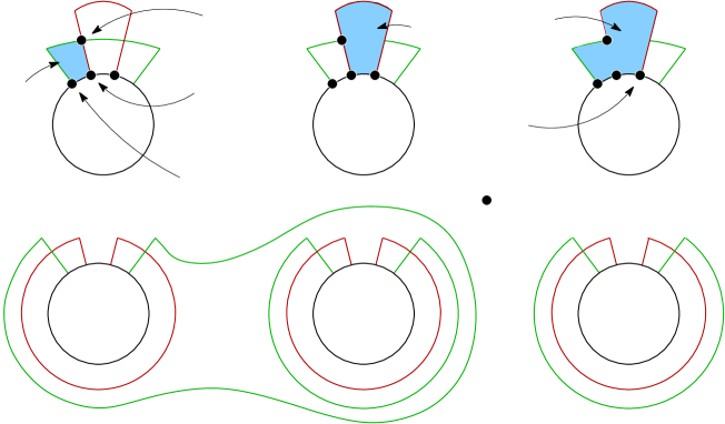
Figure 7: The Heegaard surface cut open along the $\beta$-curves.

each component we have to have a close look at the domains $\mathcal{D}_{1}$, $\mathcal{D}_{2}$ and $\mathcal{D}_{3}$. To improve the illustration in the picture we have separated them. There are exactly two domains contributing to holomorphic triangles with boundary points in $\{\widehat{\Theta}_{\beta\gamma},\widehat{\Theta}_{\gamma\delta}\}$, namely $\mathcal{D}_{1}$ and $\mathcal{D}_{3}$. The domain $\mathcal{D}_{3}$ can be written as a sum of $\mathcal{D}_{1}$ and $\mathcal{D}_{2}$, the former carrying $\mu=0$, the latter carrying $\mu=1$. Consequently, every homotopy class of triangles using $\mathcal{D}_{3}$-domains can be written as a concatenation of a triangle with a disc with the expected dimensions greater than or equal to those mentioned. Consequently, the expected dimension of the triangle using a $\mathcal{D}_{3}$-domain is strictly bigger than zero and thus does not contribute to $\widehat{F}_{\beta\gamma\delta}(\widehat{\Theta}_{\beta\gamma}\otimes\widehat{\Theta}_{\gamma\delta})$. All holomorphic triangles relevant to us have domains which are a sum of $\mathcal{D}_{1}$-domains. Taking boundary conditions into account we see that we need a $\mathcal{D}_{1}$-domain in each component. Thus, there is a unique homotopy class of triangles interesting to us. By the Riemann mapping theorem there is a unique holomorphic map $\widehat{\phi}\colon\thinspace\widehat{\mathbb{D}}\longrightarrow\Sigma$ from a surface with boundary $\widehat{\mathbb{D}}$ whose associated domain equals the sum of $\mathcal{D}_{1}$-domains. The map $\widehat{\phi}$ is a biholomorphism and thus $\widehat{\mathbb{D}}$ is a disjoint union of triangles. The uniqueness of $\widehat{\phi}$ tells us that the number of elements in the associated moduli space equals the number of non-equivalent $g$-fold branched coverings $\widehat{\mathbb{D}}\longrightarrow\mathbb{D}^{2}$. Since $\widehat{\mathbb{D}}$ is a union of $g$ discs, this covering is unique, too (up to equivalence) and thus the associated moduli space is a one-point space. ∎

Lemma 4.9 and (4.4.3) combine to give the composition law

$$\widehat{F}_{\alpha\beta\delta}=\widehat{F}_{\alpha\gamma\delta}\circ\widehat{F}_{\alpha\beta\gamma}.$$

We call a holomorphic triangle small if it is supported within the thin strips of isotopy between $\beta$ and $\delta$.

Lemma 4.10 (see [17], Lemma 9.10).

Let $F\colon\thinspace A\longrightarrow B$ be a map of filtered groups such that $F$ can be decomposed into $F_{0}+l$, where $F_{0}$ is a filtration-preserving isomorphism and $l(x)<F_{0}(x)$. Then, if the filtration on $B$ is bounded from below, the map $F$ is an isomorphism of groups.

There are two important observations to make. The first is that we can equip the chain complexes with a filtration, called the area filtration (cf. [17]), which is indeed bounded from below. In this situation the top-dimensional generator $\widehat{\Theta}_{\beta\delta}$ is generated by a single intersection point $x^{+}\in\mathbb{T}_{\beta}\cap\mathbb{T}_{\delta}$. The map $\widehat{F}_{\alpha\beta\delta}$ is induced by

$$\widehat{f}_{\alpha\beta\delta}(\,\cdot\otimes x^{+}),$$

which in turn can be decomposed into a sum of $f_{0}$ and $l$, where $f_{0}$ counts small holomorphic triangles and $l$ those triangles whose support is not contained in the thin strips of isotopy between $\beta$ and $\delta$. The map $f_{0}$ is filtration preserving and $l$, if the $\delta$-curves are close enough to the $\beta$-curves, strictly decreasing. By Lemma 4.10 the map $\widehat{F}_{\alpha\beta\delta}$ is an isomorphism between the associated Heegaard Floer homologies.
To conclude topological invariance we have to see that the following claim is true.

Theorem 4.11.

Two pointed admissible Heegaard diagrams associated to a $3$-manifold are equivalent after a finite sequence of Heegaard moves, each of them connecting two admissible Heegaard diagrams, which can be done in the complement of the base-point $z$.

The only situation where the point $z$ seems to be an obstacle arises when trying to isotope an attaching circle, $\alpha_{1}$ say, over the base-point $z$. But observe that cutting the $\alpha$-circles out of $\Sigma$ we get a sphere with holes. We can isotope $\alpha_{1}$ freely and pass the holes by handle slides. Thus, the requirement not to pass $z$ is not an obstruction at all. Instead of passing $z$ we can go the other way around the surface by isotopies and handle slides.

5 Knot Floer Homologies

Knot Floer homology is a variant of the Heegaard Floer homology of a manifold. Recall that the Heegaard diagrams used in Heegaard Floer theory come from handle decompositions relative to a splitting surface. Given a knot $K\subset Y$, we can restrict to a subclass of Heegaard diagrams by requiring the handle decomposition to come from a handle decomposition of $\overline{Y\backslash\nu K}$ relative to its boundary. Note that in the literature the knot Floer variants are defined for homologically trivial knots only. However, the definition can be carried over nearly one-to-one to give a well-defined topological invariant for arbitrary knot classes. But the generalization comes at a price. In the homologically trivial case it is possible to subdivide the groups in a special manner giving rise to a refined invariant, which cannot be defined in the non-trivial case. Given a knot $K\subset Y$, we can specify a certain subclass of Heegaard diagrams.

Definition 5.1.

A Heegaard diagram $(\Sigma,\alpha,\beta)$ is said to be subordinate to the knot $K$ if $K$ is isotopic to a knot lying in $\Sigma$ and $K$ intersects $\beta_{1}$ once, transversely and is disjoint from the other $\beta$-circles.

Since $K$ intersects $\beta_{1}$ once and is disjoint from the other $\beta$-curves we know that $K$ intersects the core disc of the $2$-handle, represented by $\beta_{1}$, once and is disjoint from the others (after possibly isotoping the knot $K$).

Lemma 5.2.

Every pair $(Y,K)$ admits a Heegaard diagram subordinate to $K$.

Proof.

By surgery theory (see [7], p. 104) we know that there is a handle decomposition of $Y\backslash\nu K$, i.e.

$$Y\backslash\nu K\cong(T^{2}\times[0,1])\cup_{\partial}h^{1}_{2}\cup_{\partial}\dots h^{1}_{g}\cup_{\partial}h^{2}_{1}\cup_{\partial}\dots\cup_{\partial}h^{2}_{g}\cup_{\partial}h^{3}$$

We close up the boundary $T^{2}\times\{0\}$ with an additional $2$-handle $h^{2*}_{1}$ and a $3$-handle $h^{3}$ to obtain

$$Y\cong h^{3}\cup_{\partial}h^{2*}_{1}\cup_{\partial}(T^{2}\times I)\cup_{\partial}h^{1}_{2}\cup_{\partial}\dots h^{1}_{g}\cup_{\partial}h^{2}_{1}\cup_{\partial}\dots\cup_{\partial}h^{2}_{g}\cup_{\partial}h^{3}.$$ (5.1)

We may interpret $h^{3}\cup_{\partial}h^{2*}_{1}\cup_{\partial}(T^{2}\times[0,1])$ as a $0$-handle $h^{0}$ and a $1$-handle $h^{1*}_{1}$. Hence, we obtain the following decomposition of $Y$:

$$h^{0}\cup_{\partial}h^{1*}_{1}\cup_{\partial}h^{1}_{2}\cup_{\partial}\dots\cup_{\partial}h^{1}_{g}\cup_{\partial}h^{2}_{1}\cup_{\partial}\dots\cup_{\partial}h^{2}_{g}\cup_{\partial}h^{3}.$$

We get a Heegaard diagram $(\Sigma,\alpha,\beta)$ where $\alpha=\alpha_{1}^{*}\cup\{\alpha_{2},\dots,\alpha_{g}\}$ are the co-cores of the $1$-handles and $\beta=\{\beta_{1},\dots,\beta_{g}\}$ are the attaching circles of the $2$-handles. ∎

Having fixed such a Heegaard diagram $(\Sigma,\alpha,\beta)$ we can encode the knot $K$ in a pair of points. After isotoping $K$ onto $\Sigma$, we fix a small interval $I$ in $K$ containing the intersection point $K\cap\beta_{1}$. This interval should be chosen small enough such that $I$ does not contain any other intersections of $K$ with other attaching curves. The boundary $\partial I$ of $I$ determines two points in $\Sigma$ that lie in the complement of the attaching circles, i.e. $\partial I=z-w$, where the orientation of $I$ is given by the knot orientation. This leads to a doubly-pointed Heegaard diagram $(\Sigma,\alpha,\beta,w,z)$. Conversely, a doubly-pointed Heegaard diagram uniquely determines a topological knot class: Connect $z$ with $w$ in the complement of the attaching circles $\alpha$ and $\beta\backslash\beta_{1}$ with an arc $\delta$ that crosses $\beta_{1}$ once. Connect $w$ with $z$ in the complement of $\beta$ using an arc $\gamma$. The union $\delta\cup\gamma$ is represents the knot klass $K$ represents. The orientation on $K$ is given by orienting $\delta$ such that $\partial\delta=z-w$. If we use a different path $\widetilde{\gamma}$ in the complement of $\beta$, we observe that $\widetilde{\gamma}$ is isotopic to $\gamma$ (in $Y$): Since $\Sigma\backslash\beta$ is a sphere with holes an isotopy can move $\gamma$ across the holes by doing handle slides. Isotope the knot along the core discs of the $2$-handles to cross the holes of the sphere. Indeed, the knot class does not depend on the specific choice of $\delta$-curve.
The knot chain complex $\widehat{\mbox{\rm CFK}}(Y,K)$ is the free $\mathbb{Z}_{2}$-module (or $\mathbb{Z}$-module) generated by the intersections $\mathbb{T}_{\alpha}\cap\mathbb{T}_{\beta}$. The boundary operator $\widehat{\partial}^{w}$, for $x\in\mathbb{T}_{\alpha}\cap\mathbb{T}_{\beta}$, is defined by

$$\widehat{\partial}^{w}(x)=\sum_{y\in\mathbb{T}_{\alpha}\cap\mathbb{T}_{\beta}}\sum_{\phi\in H(x,y,1)}\#\widehat{\mathcal{M}}_{\phi}\cdot y,$$

where $H(x,y,1)\subset\pi_{2}(x,y)$ are the homotopy classes with $\mu=1$ and $n_{z}=n_{w}=0$. We denote by $\widehat{\mbox{\rm HFK}}(Y,K)$ the associated homology theory $H_{*}(\widehat{\mbox{\rm CFK}}(Y,K),\widehat{\partial}^{w})$. The crucial observation for showing invariance is, that two Heegaard diagrams subordinate to a given knot can be connected by moves that respect the knot complement.

Lemma 5.3.

([14]) Let $(\Sigma,\alpha,\beta,z,w)$ and $(\Sigma^{\prime},\alpha^{\prime},\beta^{\prime},z^{\prime},w^{\prime})$ be two Heegaard diagrams subordinate to a given knot $K\subset Y$. Let $I$ denote the interval inside $K$ connecting $z$ with $w$, interpreted as sitting in $\Sigma$. Then these two diagrams are isomorphic after a sequence of the following moves:

1. Handle slides and isotopies among the $\alpha$-curves. These isotopies may not cross $I$.

2. Handle slides and isotopies among the $\beta_{2},\dots,\beta_{g}$. These isotopies may not cross $I$.

3. Handle slides of $\beta_{1}$ over the $\beta_{2},\dots,\beta_{g}$ and isotopies.

4. Stabilizations/destabilizations.

For the convenience of the reader we include a short proof of this lemma.

Proof.

By Theorem 4.2.12 of [7] we can transform two relative handle decompositions into each other by isotopies, handle slides and handle creation/annihilation of the handles written at the right of $T^{2}\times[0,1]$ in $(\ref{handledecomp02})$. Observe that the $1$-handles may be isotoped along the boundary $T^{2}\times\{1\}$. Thus, we can transform two Heegaard diagrams into each other by handle slides, isotopies, creation/annihilation of the $2$-handles $h^{2}_{i}$ and we may slide the $h^{1}_{i}$ over $h^{1}_{j}$ and over $h^{1*}_{1}$ (the latter corresponds to $h^{1}_{i}$ sliding over the boundary $T^{2}\times\{1\}\subset T^{2}\times I$ by an isotopy). But we are not allowed to move $h^{1*}_{1}$ off the $0$-handle. In this case we would lose the relative handle decomposition. In terms of Heegaard diagrams we see that these moves exactly translate into the moves given in ($m_{1}$) to ($m_{4}$). Just note that sliding the $h^{1}_{i}$ over $h^{1*}_{1}$, in the dual picture, looks like sliding $h^{2*}_{1}$ over the $h^{2}_{i}$. This corresponds to move ($m_{3}$). ∎

Proposition 5.4.

Let $K\subset Y$ be an arbitrary knot. The knot Floer homology group $\widehat{\mbox{\rm HFK}}(Y,K)$ is a topological invariant of the knot type of $K$ in $Y$. These homology groups split with respect to $\mbox{\rm Spin}^{c}(Y)$.

Proof.

Given one of the moves $(m_{1})$ to $(m_{4})$, the associated Heegaard Floer homologies are isomorphic, which is shown using one of the isomorphisms given in §4. Each of these maps is defined by counting holomorphic discs with punctures, whose properties are shown by defining maps by counting holomorphic discs with punctures.
Isotopies/Almost Complex Structure. Denote by $J$ the path of almost complex structures used in the definition of the Heegaard Floer homologies. Let $M$ be an isotopy or perturbation of $J$. Let $\widehat{\Phi}$ be the isomorphism induced by $M$. We split the isomorphism up into

$$\widehat{\Phi}=\widehat{\Phi}^{w}+\widehat{\Phi}^{\not=},$$

where $\widehat{\Phi}^{w}$ is defined by counting holomorphic discs with punctures (for a precise definition look into §4.2 and §4.3) that fulfill $n_{w}=0$. Let us denote with $\mathcal{M}_{0}$ the associated moduli space used to define the map $\widehat{\Phi}$. The index indicates the value of the index $\mu$. The chain map property of $\widehat{\Phi}$ was shown by counting ends of $\mathcal{M}_{1}$ which contains the same objects we needed to define $\widehat{\Phi}$ but now with the index fulfilling $\mu=1$ (see Definition 2.6). We restrict our attention to $\mathcal{M}^{w}_{0}$ and $\mathcal{M}^{w}_{1}$, the superscript $w$ indicates that we look at the holomorphic elements in $\mathcal{M}_{0}$ (or $\mathcal{M}_{1}$ respectively) with intersection number $n_{w}=0$: The additivity of the intersection number $n_{w}$ and the positivity of intersections guarantees that the ends of $\mathcal{M}^{w}_{1}$ lie within the space $\mathcal{M}^{w}_{0}$ provided that $M$ respects the point $w$. If $M$ is an isotopy, respecting $w$ means, that no attaching circle crosses the point $w$. If $M$ is a perturbation of $J$, respecting $w$ means, that we perturb $J$ through nearly symmetric almost complex structures such that $V$ (cf. Definition 2.19) also contains $\{w\}\times\mbox{\rm Sym}^{g-1}(\Sigma)$. Hence, we have the equality

$$(\partial\mathcal{M}_{1})^{w}=\partial\mathcal{M}^{w}_{1}.$$

Thus, $\widehat{\Phi}^{w}$ has to be a chain map between the respective knot Floer homologies. To show that $\widehat{\Phi}$ is an isomorphism, we invert the move $M$ we have done and construct the associated morphism $\widehat{\Psi}$. To show that $\widehat{\Psi}$ is the inverse, we construct a chain homotopy equivalence between $\widehat{\Psi}\circ\widehat{\Phi}$ and the identity (or between $\widehat{\Phi}\circ\widehat{\Psi}$ and the identity) by counting elements of $\mathcal{M}^{ch}_{0}$ which are defined by constructing a family of moduli spaces $\mathcal{M}^{\tau}_{-1}$, $\tau\in[0,1]$, and combining them to

$$\mathcal{M}^{ch}_{0}:=\bigsqcup_{\tau\in[0,1]}\mathcal{M}^{\tau}_{-1}.$$

The spaces $\mathcal{M}^{\tau}_{-1}$ are defined like done in §4.2 and §4.3. We show the chain homotopy equation by counting ends of $\mathcal{M}^{ch}_{1}$. Restricting our attention to $\mathcal{M}^{ch,w}$, this space consists of the union of spaces $\mathcal{M}^{\tau,w}_{-1}$, $\tau\in[0,1]$ (cf. §4.2 and §4.3). We obtain the equality

$$(\partial\mathcal{M}^{ch}_{0})^{w}=\partial\mathcal{M}^{ch,w}_{0}.$$

And hence we see that $\widehat{\Phi}^{w}$ is an isomorphism.
Handle slides. In case of the knot Floer homology we are able to define a pairing

$$\widehat{f}_{\alpha\beta\gamma}\colon\thinspace\widehat{\mbox{\rm CFK}}(\Sigma,\alpha,\beta,w,z)\otimes\widehat{\mbox{\rm CFK}}(\Sigma,\beta,\gamma,w,z)\longrightarrow\widehat{\mbox{\rm CFK}}(\Sigma,\alpha,\gamma,w,z)$$

induced by a doubly-pointed Heegaard triple diagram $(\Sigma,\alpha,\beta,\gamma,w,z)$. We have to see, that in case the triple is induced by a handle slide, the knot Floer homology $\widehat{\mbox{\rm HFK}}(\Sigma,\beta,\gamma,w,z)$ carries a top-dimensional generator $\widehat{\Theta}_{\beta\gamma}$, analogous to the discussion for the Heegaard Floer homologies, with similar properties (recall the composition law). It is easy to observe that, in case of a handle slide, the points $w$ and $z$ lie in the same component of $\Sigma\backslash\{\beta\cup\gamma\}$. Hence, we have an identification

$$\widehat{\mbox{\rm HFK}}(\Sigma,\beta,\gamma,w,z)=\widehat{\mbox{\rm HF}}(\#^{g}(\mathbb{S}^{2}\times\mathbb{S}^{1})).$$

Counting triangles with $n_{w}=0$, the positivity of intersections and the additivity of the intersection number $n_{w}$ guarantees that the discussion carries over verbatim and gives invariance here. ∎

Remark.

If a handle were slid over $\beta_{1}$, we would leave the class of subordinate Heegaard diagrams. Recall that subordinate Heegaard diagrams come from relative handle decompositions.

5.0.1 Admissibility

The admissibility condition given in Definition 2.17 suffices to give a well-defined theory. However, since we have an additional point $w$ in play, we can relax the admissibility condition.

Definition 5.5.

We call a doubly-pointed Heegaard diagram $(\Sigma,\alpha,\beta,w,z)$ extremely weakly admissible for the $\mbox{\rm Spin}^{c}$-structure $s$ if for every non-trivial periodic domain, with $n_{w}=0$ and $\left<c_{1}(s),\mathcal{H}(\mathcal{D})\right>=0$, the domain has both positive and negative coefficients.

With a straightforward adaptation of the proof of well-definedness in the case of $\widehat{\partial}_{z}$ we get the following result (see [17], Lemma 4.17, cf. Definition 2.17 and cf. proof of Theorem 2.3).

Theorem 5.6.

Let $(\Sigma,\alpha,\beta,w,z)$ be an extremely weakly admissible Heegaard diagram. Then $\widehat{\partial}^{w}$ is well-defined and a differential. $\square$

Note that Ozsváth and Szabó impose weak admissibility of the Heegaard diagram $(\Sigma,\alpha,\beta,z)$. The introduction of our relaxed condition is done since we there are setups (see [26]) where it is convenient to relax the admissibility condition like introduced.

5.0.2 Other knot Floer homologies

By permitting variations of $n_{z}$ in the differential we define the homology $\mbox{\rm HFK}^{-}$: Let $\mbox{\rm CFK}^{-}(Y,K)$ be the $\mathbb{Z}[U^{-1}]$-module (or $\mathbb{Z}_{2}[U^{-}{1}]$-module) generated by the intersection points $\mathbb{T}_{\alpha}\cap\mathbb{T}_{\beta}$. A differential $\partial^{-}_{w}$ is defined by

$$\partial^{-}_{w}(x)=\sum_{y\in\mathbb{T}_{\alpha}\cap\mathbb{T}_{\beta}}\sum_{\phi\in H(x,y,1)}\#\widehat{\mathcal{M}}_{\phi}\cdot y,$$

where $H(x,y,1)\subset\pi_{2}(x,y)$ are the homotopy classes with $n_{w}=0$ (possibly $n_{z}\not=0$) and $\mu=1$. To make this a well-defined map we may impose the strong admissibility condition on the underlying Heegaard diagram or relax it like it was done for weak admissibility in Definition 5.5. Using this construction, and continuing like in §3, we define variants we denote by $\mbox{\rm HFK}^{\infty}$ and $\mbox{\rm HFK}^{+}$. The groups are naturally connected by exact sequences analogous to those presented in Lemma 3.3.

5.1 Refinements

If the knot $K$ is null-homologous, we get, using a Mayer-Vietoris computation, that

$$\mbox{\rm Spin}^{c}(Y_{0}(K))=\mbox{\rm Spin}^{c}(Y)\times\mathbb{Z}.$$ (5.2)

Alternatively, by interpretation of $\mbox{\rm Spin}^{c}$-structures as homology classes of vector fields, i.e. homotopy classes over the $2$-skeleton of $Y$, we can prove this result and see that there is a very geometric realization of the correspondence (5.2). Given a $\mbox{\rm Spin}^{c}$-structure $t$ on $Y_{0}(K)$, we associate to it the pair $(s,k)$, where $s$ is the restriction of $t$ on $Y$ and $k$ an integer we will define in a moment. Beforehand, we would like to say in what way the phrase restriction of $t$ onto $Y$ makes sense. Pick a vector field $v$ in the homology class of $t$ and restrict this vector field to $Y\backslash\nu K$. Observe that we may regard $Y\backslash\nu K$ as a submanifold of $Y_{0}(K)$. The restricted vector field may be interpreted as sitting on $Y$. We extend $v$ to the tubular neighborhood $\nu K$ of $K$ in $Y$, which determines a $\mbox{\rm Spin}^{c}$-structure $s$ on $Y$. However, the induced $\mbox{\rm Spin}^{c}$-structure does not depend on the special choice of extension of $v$ on $\nu K$, since $K$ is homologically trivial.
To a $\mbox{\rm Spin}^{c}$-structure $t$ we can associate a link $L_{t}$ and its homology class determines the $\mbox{\rm Spin}^{c}$-structure. Denote by $\mu_{0}$ a meridian of $K$ in $Y$, interpreted as sitting in $Y_{0}(K)$. Then $L_{t}$ can be written as a sum

$$L_{t}=k\cdot\mu_{0}+\dots,$$

and thus we can compute $k$ with

$$k=lk^{Y}(L,\lambda)=\#^{Y}(L,F)=\#^{Y_{0}(K)}(L,\widehat{F})=\bigl{<}\frac{1}{2}c_{1}(t),[\widehat{F}]\bigr{>},$$

where $\lambda$ is a push-off of $K$ in $Y$ and $\widehat{F}$ is obtained by taking a Seifert surface $F$ of $K$ in $Y$ and capping it off with a disc in $Y_{0}(K)$.
We can try to separate intersection points $\mathbb{T}_{\alpha}\cap\mathbb{T}_{\beta}$ with respect to $\mbox{\rm Spin}^{c}$-structures of $Y_{0}(K)$. This defines a refined invariant $\widehat{\mbox{\rm CFK}}(Y,K,t)$, for $t\in\mbox{\rm Spin}^{c}(Y_{0}(K))$, and we have

$$\widehat{\mbox{\rm CFK}}(Y,K,s)=\bigoplus_{t\in H_{s}}\widehat{\mbox{\rm CFK}}(Y,K,t),$$

where $H_{s}\subset\mbox{\rm Spin}^{c}(Y_{0}(K))$ are the elements extending $s\in\mbox{\rm Spin}^{c}(Y)$. We have to show that $\widehat{\partial}^{w}$ preserves this splitting. We point the interested reader to [14].

6 Maps Induced By Cobordisms

The pairing introduced in §4.4.1 can be used to associate maps to cobordisms. In general, every cobordism between two connected $3$-manifolds $Y$ and $Y^{\prime}$ can be decomposed into $1$-handles, $2$-handles and $3$-handles (cf. Proposition 4.2.13 in [7]). All cobordisms appearing through our work will be induced by surgeries on a $3$-manifold. A surgery corresponds to a $2$-handle attachment to the trivial cobordism $Y\times I$. For this reason we will not discuss $1$-handles and $3$-handles. We will give the construction for cobordisms obtained by attachments of one single $2$-handle. For a definition of the general, very similar construction, we point the interested reader to [19].
Given a framed knot $K\subset Y$, we fix an admissible Heegaard diagram subordinate to $K$. Without loss of generality, we can choose the diagram such that $\beta_{1}=\mu$ is a meridian of the first torus component of $\Sigma$. The framing of $K$ is given, by pushing $K$ off itself onto the Heegaard surface. The resulting knot on $\Sigma$ is determined by $\lambda+n\cdot\mu$, for a suitable $n\in\mathbb{Z}$. With this done, we can represent the surgery by the Heegaard triple diagram $(\Sigma,\alpha,\beta,\gamma)$ where $\gamma_{i}$, $i\geq 2$, are isotopic push-offs of the $\beta_{i}$, perturbed, such that $\gamma_{i}$ intersects $\beta_{i}$ in a pair of cancelling intersection points. The curve $\gamma_{1}$ equals $\lambda+n\cdot\mu$.

Proposition 6.1.

The cobordism $X_{\alpha\beta\gamma}\cup_{\partial}(\#^{g-1}D^{3}\times\mathbb{S}^{1})$ is diffeomorphic to the cobordism $W_{K}$ given by the framed surgery along $K$.

We define

$$\widehat{F}_{W_{K}}=\widehat{f}_{\alpha\beta\gamma}^{*}$$

as the map induced by the cobordism $W_{K}$. Of course, for this to make sense, we have to show that $\widehat{F}_{W_{K}}$ does not depend on the choices made in its definition. This is shown by the following recipe: Suppose we are given maps $\widehat{F}_{1}$ and $\widehat{F}_{2}$, induced by two sets of data that can be connected via a Heegaard move. Then these maps fit into a commutative box

$$\begin{diagram}$$

where the associated Heegaard Floer homologies are connected by the isomorphism induced by the move done to connect the diagrams. If we did a handle slide, we use associativity together with a conservation property analogous to Lemma 4.9 to show a composition law reading

$$\widehat{F}_{\alpha\gamma\gamma^{\prime}}\circ\widehat{F}_{\alpha\beta\gamma}=\widehat{F}_{\alpha\beta\gamma^{\prime}}.$$

In a similar vein one covers handle slides among the $\alpha$-circles. Invariance under Isotopies and changes of almost complex structures is shown by proving, that the isomorphisms induced by these moves make the corresponding diagram commute.
Given a framed link $L=K_{1}\sqcup\dots\sqcup K_{m}$, observe that we can obviously define a map

$$\widehat{F}_{L}\colon\thinspace\widehat{\mbox{\rm HF}}(Y)\longrightarrow\widehat{\mbox{\rm HF}}(Y_{L}),$$

where $Y_{L}$ is the manifold obtained by surgery along $L$ in $Y$, in the same way we did for a single attachment. We claim that associativity, together with a conservation law like given in Lemma 4.9, will suffice to show that the map $\widehat{F}_{L}$ associated to multiple attachments is a composition

$$\widehat{F}_{L}=\widehat{F}_{K_{m}}\circ\dots\circ\widehat{F}_{K_{1}}$$

of the maps $\widehat{F}_{K_{i}}$ associated to the single attachments along the $K_{i}$. The associativity will prove that the maps in this chain commute. Although we have to be careful by saying they commute. The maps, as we change the order of the attachments, are defined differently and, thus, differ depending on the attachment order.
There is a procedure for defining maps associated to $1$-handle attachments and $3$-handle attachments. Their construction is not very enlightening, and the cobordisms appearing in our discussions will mostly be induced by surgeries.

7 The Surgery Exact Triangle

Denote by $K$ a knot in $Y$ and let $n$ be a framing of that knot. We will briefly recall the notion of framings to fix the notation. Given a tubular neighborhood $\nu K\hookrightarrow Y$ of $K$, we fix a meridian $\mu$ of the boundary $\partial\nu K$. A framing is given by a push-off $n$ of $K$, sitting on $\partial\nu K$, such that $\#(\mu,n)=1$. The pair $\mu,\lambda$ determines a basis for $H_{1}(\partial\nu K;\mathbb{Z})$. Any other framing $\lambda^{\prime}$ can be written as $\lambda^{\prime}=m\cdot\mu+\lambda$, for an integer $m\in\mathbb{Z}$, and vice versa any of these linear combinations determines a framing on $K$. Thus, when writing $n$ as a framing for $K$ it makes sense to talk about the framing $n+\mu$. If the knot is homologically trivial, it bounds a Seifert surface which naturally induces a framing on the knot called the Seifert framing. This serves as a canonical framing, and having fixed this framing we can talk about framings as an integer $n\in\mathbb{Z}$. This identification will be done whenever it makes sense.
There is a long exact sequence

$$\dots\overset{\partial_{*}}{\longrightarrow}\widehat{\mbox{\rm HF}}(Y)\overset{\widehat{F}_{1}}{\longrightarrow}\widehat{\mbox{\rm HF}}(Y_{K}^{n})\overset{\widehat{F}_{2}}{\longrightarrow}\widehat{\mbox{\rm HF}}(Y_{K}^{n+\mu})\overset{\partial_{*}}{\longrightarrow}\dots,$$ (7.1)

where $\widehat{F}_{i}$ denote the maps associated to the cobordisms induced by the surgeries. The map $\widehat{F}_{2}$ is induced by a surgery along a meridian of $K$ with framing $-1$. The exactness of the sequence is proved by showing that $\widehat{F}_{1}$ – on the chain level – can be perturbed within its chain homotopy class to fit into a short exact sequence of chain complexes and chain maps (see [18])

$$0\longrightarrow\widehat{\mbox{\rm CF}}(Y)\overset{\widetilde{\widehat{F}_{1}}}{\longrightarrow}\widehat{\mbox{\rm CF}}(Y_{K}^{n})\overset{\widehat{F}_{2}}{\longrightarrow}\widehat{\mbox{\rm CF}}(Y_{K}^{n+\mu})\longrightarrow 0.$$ (7.2)

The map $\partial_{*}$ in (7.1) denotes the induced coboundary. This enables us to prove the existence of the surgery exact triangle.

Theorem 7.1.

In the situation described above, let $\nu$ denote a meridian of $\mu$ and $\widehat{F}_{3}$ the map induced by surgery along $\nu$ with framing $-1$. There is a long exact sequence which is called surgery exact triangle.

2pt $n$ [Bl] at 3 182 $n\!+\!\mu$ [Bl] at 93 182 $n$ [Bl] at 175 182 $n$ [Bl] at 323 182 $n$ [Bl] at 463 182 $n$ [Bl] at 624 182 $n$ [Bl] at 723 182 $K$ [l] at 3 8 $K$ [l] at 93 8 $K$ [l] at 175 8 $K$ [l] at 323 8 $K$ [l] at 463 8 $K$ [l] at 624 8 $K$ [l] at 723 8 $-1$ [t] at 143 80 $0$ [t] at 294 80 $-1$ [t] at 431 80 $-1$ [t] at 595 80 $\mu$ [B] at 143 101 $\mu$ [B] at 294 101 $\mu$ [B] at 431 101 $\mu$ [B] at 595 101 $\nu$ [l] at 516 110 $-1$ [Bl] at 495 127 $\nu$ [l] at 679 110 $0$ [Bl] at 663 127

Figure 8: The topological situation in the exact triangle.

Proof.

Observe that the topological situation is very symmetric. The long exact sequence (7.1) corresponds to the topological situation pictured in Figure 8. Each arrow in Figure 8 corresponds to an exact sequence of type (7.1). With the identifications given, we can concatenate the three sequences to give the surgery exact sequence of Theorem 7.1. ∎

A second proof, one more appealing to our aesthetic sense, although only valid for $\mathbb{Z}_{2}$-coefficients, was also developed by Ozsváth and Szabó. We will discuss the proof in the remainder of this paragraph. It contains a very interesting algebraic approach for showing exactness of a sequence.
The composition $\widehat{f}_{2}\circ\widehat{f}_{1}$ in the sequence

$$\widehat{\mbox{\rm CF}}(Y)\overset{\widehat{f}_{1}}{\longrightarrow}\widehat{\mbox{\rm CF}}(Y_{K}^{n})\overset{\widehat{f}_{2}}{\longrightarrow}\widehat{\mbox{\rm CF}}(Y_{K}^{n+\mu})$$ (7.3)

is null-chain homotopic. Let $(\Sigma,\alpha,\beta,z)$ be a Heegaard diagram subordinate to the knot $K\subset Y$. We can choose the data such that $\beta_{1}$ is a meridian of the first torus component of $\Sigma$. A Heegaard diagram of $Y_{K}^{n}$ can be described by $(\Sigma,\alpha,\gamma,z)$ where $\gamma_{i}$, $i\geq 2$ are isotopic push-offs of the $\beta_{i}$ such that $\beta_{i}$ and $\gamma_{i}$ meet in two cancelling intersections transversely. The curve $\gamma_{1}$ equals $n\cdot\beta_{1}+\lambda$ where $\lambda$ is the longitude of the first torus component of $\Sigma$ determining the framing on $K$. We define a fourth set of attaching circles $\delta$ where $\delta_{i}$, $i\geq 2$ are push-offs of the $\gamma_{i}$ which meet the $\gamma_{i}$ and $\delta_{i}$ in two cancelling intersections. The curve $\delta_{1}$ equals $(n+1)\beta_{1}+\lambda$. Thus, $(\Sigma,\alpha,\delta)$ is a Heegaard diagram of $Y_{K}^{n+\mu}$. By associativity (4.8), the composition $\widehat{f}_{2}\circ\widehat{f}_{1}$ is chain homotopic to

$$\widehat{f}_{\alpha\beta\delta}(\,\cdot\otimes\widehat{f}_{\beta\gamma\delta}(\widehat{\Theta}_{\beta\gamma}\otimes\widehat{\Theta}_{\gamma\delta})),$$

where the chain homotopy $H$ is given by counting holomorphic rectangles with suitable boundary conditions (cf. §4.4). To compute $\widehat{f}_{\beta\gamma\delta}(\widehat{\Theta}_{\beta\gamma}\otimes\widehat{\Theta}_{\gamma\delta})$ we use a model calculation. Figure 9 illustrates the Heegaard triple diagram.

2pt $\widehat{\Theta}_{\beta\gamma}$ [B] at 268 202 $\widehat{\Theta}_{\gamma\delta}$ [B] at 348 228 $z$ [l] at 233 162 $\delta_{1}$ [t] at 4 52 $\beta_{1}$ [l] at 95 16 $\widehat{\Theta}_{\gamma\delta}$ [l] at 145 10 $\gamma_{1}$ [t] at 183 45 $\beta_{2}$ [t] at 254 37 $\gamma_{2}$ [t] at 275 32 $\delta_{2}$ [t] at 294 20

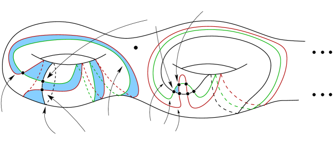
Figure 9: Heegaard triple diagram for computation of $\widehat{f}_{\beta\gamma\delta}(\widehat{\Theta}_{\beta\gamma}\otimes\widehat{\Theta}_{\gamma\delta})$.

There are exactly two homotopy classes of Whitney triangles we have to count. Each domain associated to the homotopy classes is given by a disjoint union of triangles. Thus, the moduli spaces associated to these homotopy classes each carry one single element (cf. Lemma 4.9). Hence, in $\mathbb{Z}_{2}$-coefficients

$$\widehat{f}_{\beta\gamma\delta}(\widehat{\Theta}_{\beta\gamma}\otimes\widehat{\Theta}_{\gamma\delta})=2\cdot\widehat{\Theta}_{\beta\delta}=0.$$

In general we have to see that we can choose the signs of the associated elements differently. But observe that the domains of both homotopy classes contributing in our signed count differ by a triply-periodic domain. We can choose the signs on these elements differently.
This discussion carries over verbatim for any of the maps in the surgery exact sequence. The symmetry of the situation, as indicated in Figure 8, makes it possible to carry over the proof given here.
There is an algebraic trick to show exactness on the homological level. Let

$$H\colon\thinspace\widehat{\mbox{\rm CF}}(Y)\longrightarrow\widehat{\mbox{\rm CF}}(Y_{K}^{n+\mu})$$

denote the null-homotopy of $\widehat{f}_{2}\circ\widehat{f}_{1}$ (cf. §4.4). Define the chain complex $A_{\widehat{f}_{1},\widehat{f}_{2}}$ to be given by the module $A=\widehat{\mbox{\rm CF}}(Y)\oplus\widehat{\mbox{\rm CF}}(Y_{K}^{n})\oplus\widehat{\mbox{\rm CF}}(Y_{K}^{n+\mu})$ with the differential

$$\partial=\left(\begin{matrix}\widehat{\partial}_{Y}&0&0\\ \widehat{f}_{1}&\widehat{\partial}_{Y_{K}^{n}}&0\\ H&\widehat{f}_{2}&\widehat{\partial}_{Y_{K}^{n+\mu}}\end{matrix}\right).$$

Lemma 7.2.

The sequence (7.3) is exact on the homological level at $\widehat{\mbox{\rm CF}}(Y_{K}^{n})$ if $H_{*}(A_{\widehat{f}_{1},\widehat{f}_{2}})=0$.

Proof.

Suppose we are given an element $b\in\widehat{\mbox{\rm CF}}(Y_{K}^{n})\cap\ker(\widehat{f}_{2})$ with $\widehat{\partial}_{Y_{K}^{n}}b=0$. Since $H_{*}(A_{\widehat{f}_{1},\widehat{f}_{2}},\partial)$ is trivial there is an element $(x,y,w)\in A$ such that $(0,b,0)=\partial(x,y,w)$. Thus, we have

$$b=\widehat{f}_{1}(x)+\widehat{\partial}_{Y_{K}^{n}}(y)$$

proving, that $[b]\in\mbox{\rm im}(\widehat{F}_{1})$. ∎

Definition 7.3.

For a chain map $f\colon\thinspace A\longrightarrow B$ between $\mathbb{Z}_{2}$-vector spaces we define its mapping cone to be the chain complex $M(f)$, given by the module $A\oplus B$ with differential

$$\partial_{f}=\left(\begin{matrix}\partial_{A}&0\\ f&\partial_{B}\end{matrix}.\right)$$

The mapping cone is a chain complex.

From the definition of mapping cones there is a short exact sequence of chain complexes

$$0\longrightarrow\widehat{\mbox{\rm CF}}(Y_{K}^{n+\mu})\overset{\widehat{f}_{1}}{\longrightarrow}A_{\widehat{f}_{1},\widehat{f}_{2}}\overset{\widehat{f}_{2}}{\longrightarrow}M(\widehat{f}_{1})\longrightarrow 0$$

inducing a long exact sequence between the associated homologies. The connecting morphism of this long exact sequence is induced by

$$(H,\widehat{f}_{2})\colon\thinspace M(\widehat{f}_{1})\longrightarrow\widehat{\mbox{\rm CF}}(Y_{K}^{n+\mu}).$$

The triviality of $H_{*}(A_{\widehat{f}_{1},\widehat{f}_{2}},\partial)$ is the same as saying that $(H,\widehat{f}_{2})_{*}$ is an isomorphism.

Lemma 7.4 ([20], Lemma 4.2).

Let $\{A_{i}\}_{i\in\mathbb{Z}}$ be a collection of modules and let

$$\{f_{i}\colon\thinspace A_{i}\longrightarrow A_{i+1}\}_{i\in\mathbb{Z}}$$

be a collection of chain maps such that $f_{i+1}\circ f_{i}$, $i\in\mathbb{Z}$ is chain homotopically trivial by a chain homotopy $H_{i}\colon\thinspace A_{i}\longrightarrow A_{i+2}$. The maps

$$\psi_{i}=f_{i+2}\circ H_{i}+H_{i+1}\circ f_{i}\colon\thinspace A_{i}\longrightarrow A_{i+3}$$

should induce isomorphisms between the associated homologies. Then the maps $(H_{i},f_{i+1})\colon\thinspace M(f_{i})\longrightarrow A_{i+2}$ induce isomorphisms on the homological level.

If we can show that the sequence

$$\dots\overset{\widehat{f}_{3}}{\longrightarrow}\widehat{\mbox{\rm CF}}(Y)\overset{\widehat{f}_{1}}{\longrightarrow}\widehat{\mbox{\rm CF}}(Y_{K}^{n})\overset{\widehat{f}_{2}}{\longrightarrow}\widehat{\mbox{\rm CF}}(Y_{K}^{n+\mu})\overset{\widehat{f}_{3}}{\longrightarrow}\dots$$

satisfies the assumptions of Lemma 7.4, then for every pair $\widehat{f}_{i}$ and $\widehat{f}_{i+1}$, the associated map $(H,\widehat{f}_{i+1})_{*}$ is an isomorphism. With the arguments from above, i.e. analogous to Lemma 7.2, we conclude that $\mbox{\rm im}(\widehat{F}_{i})=\ker(\widehat{F}_{i+1})$. Hence, Theorem 7.1 follows.

8 The Contact Element and $\widehat{\mathcal{L}}$

8.1 Contact Structures

A $3$-dimensional contact manifold is a pair $(Y,\xi)$ where $Y$ is a $3$-dimensional manifold and $\xi\subset TY$ a hyperplane bundle that can be written as the kernel of a $1$-form $\alpha$ with the property

$$\alpha\wedge d\alpha\not=0.$$ (8.1)

Those $1$-forms satisfying $(\ref{contcond})$ are called contact forms. Given a contact manifold $(Y,\xi)$, the associated contact form is not unique. Suppose $\alpha$ is a contact form of $\xi$ then, given a non-vanishing function $\lambda\colon\thinspace Y\longrightarrow\mathbb{R}^{+}$, we can change the contact form to $\lambda\alpha$ without affecting the contact condition (8.1):

$$\lambda\alpha\wedge d(\lambda\alpha)=\lambda\alpha\wedge d\lambda\wedge\alpha+\lambda^{2}\alpha\wedge d\alpha=\lambda^{2}\alpha\wedge d\alpha\not=0.$$

The existence of a contact form implies that the normal direction $TY/\xi$ is trivial. We define a section $R_{\alpha}$ by

$$\alpha(R_{\alpha})\not=0\;\mbox{\rm and }\;\;\iota_{R_{\alpha}}d\alpha=0.$$

This vector field is called Reeb field of the contact form $\alpha$. The contact condition implies that $d\alpha$ is a non-degenerate form on $\xi$. Thus, $\iota_{R_{\alpha}}d\alpha=0$ implies that for each point $p\in Y$ the vector $(R_{\alpha})_{p}$ is an element of $T_{p}Y\backslash\xi_{p}$. Thus, $R_{\alpha}$ is a section of $TY/\xi$.

Definition 8.1.

Two contact manifolds $(Y,\xi)$ and $(Y^{\prime},\xi^{\prime})$ are called contactomorphic if there is a diffeomorphism $\phi\colon\thinspace Y\longrightarrow Y^{\prime}$ preserving the contact structures, i.e. such that $T\phi(\xi)=\xi^{\prime}$. The map $\phi$ is a contactomorphism.

It is a remarkable property of contact manifolds that there is a unique standard model for these objects.

Definition 8.2.

The pair $(\mathbb{R}^{3},\xi_{std})$, where $\xi_{std}$ is the contact structure given by the kernel of the $1$-form $dz-y\,dx$, is called standard contact space.

Every contact manifold is locally contactomorphic to the standard contact space. This is known as Darboux’s theorem. As a consequence we will not be able to derive contact invariants by purely local arguments, in contrast to differential geometry where for instance curvature is a constraint to the existing local model.

Theorem 8.3 (Gray Stability, cf. [6]).

Each smooth homotopy of contact structures $(\xi_{t})_{t_{\in}[0,1]}$ is induced by an ambient isotopy $\phi_{t}$, i.e. the condition $T\phi_{t}(\xi_{0})=\xi_{t}$ applies for all $t\in[0,1]$.

An isotopy induced homotopy of contact structures is called contact isotopy. So, a homotopy of contact structures can be interpreted as an isotopy and, vice versa, an isotopy induces a homotopy of contact structures. As in the case of vector fields, we have a natural connection to isotopies, i.e. objects whose existence and form will be closely related to the manifold’s topology.
A contact vector field $X$ is a vector field whose local flow preserves the contact structure. An embedded surface $\Sigma\hookrightarrow Y$ is called convex if there is a neighborhood of $\Sigma$ in $Y$ in which a contact vector field exists that is transverse to $\Sigma$. The existence of a contact vector field immediately implies that there is a neighborhood $\Sigma\times\mathbb{R}\hookrightarrow Y$ of $\Sigma$ in which the contact structure is invariant in $\mathbb{R}$-direction. Thus, convex surfaces are the objects along which we glue contact manifolds together.

Definition 8.4.

A knot $K\subset Y$ is called Legendrian if it is tangent to the contact structure.

The contact condition implies that, on a $3$-dimensional contact manifold $(Y,\xi)$, only $1$-dimensional submanifolds, i.e. knots and links, can be tangent to $\xi$. Every Legendrian knot admits a tubular neighborhood with a convex surface as boundary. Hence, it is possible to mimic surgical constructions to define the contact geometric analogue of surgery theory, called contact surgery. Contact surgery in arbitrary dimensions was introduced by Eliashberg in [4]. His construction, in dimension $3$, corresponds to $(-1)$-contact surgeries. For $3$-dimensional contact manifolds Ding and Geiges gave in [2] a definition of contact-$r$-surgeries (cf. also [3]) for arbitrary $r\in\mathbb{Q}>0$. It is nowadays one of the most significant tools for $3$-dimensional contact geometry. Its importance relies in the following theorem.

Theorem 8.5 (see [3]).

Given a contact manifold $(Y,\xi)$, there is a link $\mathbb{L}=\mathbb{L}^{+}\sqcup\mathbb{L}^{-}$ in $\mathbb{S}^{3}$ such that contact-$(+1)$-surgery along the link $\mathbb{L}^{+}$ and contact-$(-1)$-surgery along $\mathbb{L}^{-}$ in $(\mathbb{S}^{3},\xi_{std})$ yields $(Y,\xi)$.

Moreover, if we choose cleverly, we can accomplish $\mathbb{L}^{+}$ to have just one component. Using $(-1)$-contact surgeries only, we can transform an arbitrary overtwisted contact manifold into an arbitrary (not necessarily overtwisted) contact manifold. For a definition of overtwistedness we point the reader to [6]. Thus, starting with a knot $K$ so that $(+1)$-contact surgery along $K$ yields an overtwisted contact manifold $(Y^{\prime},\xi^{\prime})$, for any contact manifold $(Y,\xi)$, we can find a link $\mathbb{L}^{-}$, such that $(-1)$-contact surgery along $\mathbb{L}^{-}$ in $(Y^{\prime},\xi^{\prime})$ yields $(Y,\xi)$. An example for such a knot $K$ is the Legendrian shark, i.e. the Legendrian realization of the unknot with $tb=-1$ and $rot=0$.

8.2 Open Books

For a detailed treatment of open books we point the reader to [5].

Definition 8.6.

An open book on a closed, oriented $3$-manifold $Y$ is a pair $(B,\pi)$ defining a fibration

$$P\hookrightarrow Y\backslash B\overset{\pi}{\longrightarrow}\mathbb{S}^{1},$$

where $P$ is an oriented surface with boundary $\partial P=B$. For every component $B_{i}$ of $B$ there is a neighborhood $\iota\colon\thinspace D^{2}\times\mathbb{S}^{1}\hookrightarrow\nu B_{i}\subset Y$ such that the core $C=\{0\}\times\mathbb{S}^{1}$ is mapped onto $B_{i}$ under $\iota$ and $\pi$ commutes with the projection $(D^{2}\times\mathbb{S}^{1})\backslash C\longrightarrow\mathbb{S}^{1}$ given by $(r\cdot\exp(it),\exp(is))\longmapsto\exp(it)$. The submanifold $B$ is called binding and $P$ the page of the open book.

An abstract open book is a pair $(P,\phi)$ consisting of an oriented genus-$g$ surface $P$ with boundary and a homeomorphism $\phi\colon\thinspace P\longrightarrow P$ that is the identity near the boundary of $P$. The surface $P$ is called page and $\phi$ the monodromy. Given an abstract open book $(P,\phi)$, we may associate to it a $3$-manifold. Let $c_{1},\dots,c_{k}$ denote the boundary components of $P$. Observe that

$$(P\times[0,1])/(p,1)\sim(\phi(p),0)$$ (8.2)

is a $3$-manifold. Its boundary is given by the tori

$$\left((c_{i}\times[0,1])/(p,1)\sim(p,0)\right)\cong c_{i}\times\mathbb{S}^{1}.$$

Fill in each of the holes with a full torus $\mbox{\rm D}^{2}\times\mathbb{S}^{1}$: we glue a meridional disc $\mbox{\rm D}^{2}\times\{\star\}$ onto $\{\star\}\times\mathbb{S}^{1}\subset c_{i}\times\mathbb{S}^{1}$. In this way we define a closed, oriented $3$-manifold $Y(P,\phi)$. Denote by $B$ the union of the cores of the tori $\mbox{\rm D}^{2}\times\mathbb{S}^{1}$. The set $B$ is called binding. By definition of abstract open books we obtain an open book structure

$$P\hookrightarrow Y(P,\phi)\backslash B\longrightarrow\mathbb{S}^{1}$$

on $Y(P,\phi)$. Conversely, given an open book by cutting a small tubular neighborhood $\nu B$ out of $Y$, we obtain a $P$-bundle over $\mathbb{S}^{1}$. Thus, there is a homeomorphism $\phi\colon\thinspace P\longrightarrow P$ such that

$$Y\backslash\nu B\cong(P\times[0,1])/(p,1)\sim(\phi(p),0).$$

Inside the standard neighborhood $\nu B$, as given in the definition, the homeomorphism $\phi$ is the identity. So, the pair $(P,\phi)$ defines an abstract open book.

Definition 8.7.

Two abstract open books $(P,\phi)$ and $(P,\phi^{\prime})$ are called equivalent if there is a homeomorphism $h\colon\thinspace P\longrightarrow P$, which is the identity near the boundary, such that $\phi\circ h=\phi^{\prime}\circ h$. We denote by $\mbox{\rm ABS}(Y)$ the set of abstract open books $(P,\phi)$ with $Y(P,\phi)=Y$, up to equivalence.

Two open books are called equivalent if they are diffeomorphic. The set of equivalence classes of open books is denoted by $\mbox{\rm OB}(Y)$. An abstract open book defines an open book up to diffeomorphism. With the construction given above we define a map

$$\Psi\colon\thinspace\mbox{\rm ABS}(Y)\longrightarrow\mbox{\rm OB}(Y)$$

and its inverse. Thus, to some point, open books and abstract open books are the same objects. Sometimes, it is more convenient to deal with abstract open books rather than open books themselves.

8.3 Open Books, Contact Structures and Heegaard Diagrams

Given an open book $(B,\pi)$ or an abstract open book $(P,\phi)$, define a surface $\Sigma$ by gluing together two pages at their boundary

$$\Sigma=P_{1/2}\cup_{\partial}P_{1}.$$

The manifold $Y$ equals the union $H_{0}\cup H_{1}$ where $H_{i}=\pi^{-1}([i/2,(i+1)/2])$, $i=0,1$. Any curve $\gamma$ in $Y$ running from $H_{0}$ to $H_{1}$, when projected onto $\mathbb{S}^{1}$, has to intersect $\{1/2,1\}$ at some point. Thus, the curve $\gamma$ is forced to intersect $\Sigma$. The submanifolds $H_{i}$ are handlebodies of genus $g(\Sigma)$ and

$$Y=H_{0}\cup_{\partial}H_{1}$$

is a Heegaard decomposition of $Y$.

Definition 8.8.

A system $a=\{a_{1},\dots,a_{n}\}$ of disjoint, properly embedded arcs on $P$ is called cut system if $P\backslash\{a_{1},\dots,a_{n}\}$ is topologically a disc.

A system of arcs is a cut system if and only if it defines a basis for the first homology of $(P,\partial P)$.
We interpret the curve $a_{i}$ as sitting on $P_{1/2}$ and $\overline{a_{i}}$, i.e. the curve $a_{i}$ with reversed orientation, as sitting inside $P_{1}$. These two can be combined to $\alpha_{i}=a_{i}\cup_{\partial}\overline{a_{i}}$, $i=1,\dots,n$, which all sit in $\Sigma$. Referring to the relation between open books and abstract open books discussed in §8.2, observe that

$$H_{1}=\pi^{-1}([1/2,1])=(P\times[1/2,1])/\!\!\sim$$

where $\sim$ identifies points $(p,0)$ with $(\phi(p),1)$ for $p\in P$ and points $(p,t)$ with $(p,t^{\prime})$ for $p\in\partial P$ and $t,t^{\prime}\in[1/2,1]$. Thus $a_{i}\times[1/2,1]$ determines a disc in $H_{1}$ whose boundary is $\alpha_{i}$. This means we can interpret the set $\{\alpha_{1},\dots,\alpha_{n}\}$ as a set of attaching circles for the handlebody $H_{1}$. The gluing of the two handlebodies $H_{0}$ and $H_{1}$ is given by the pair $(id,\phi)$ where $id$ is the identity on $P_{1/2}$ and $\phi$ the monodromy, interpreted as a map $P_{1}\longrightarrow P_{0}$. These two maps combine to a map $\partial H_{1}\longrightarrow\partial H_{0}$. Define $b_{i}$, $i=1,\dots,n$, as small push-offs of the $a_{i}$ that intersect these transversely in a single point (see Figure 10). Then by the gluing of the two handlebodies $H_{0}$ and $H_{1}$ the $\alpha$-curves define a Heegaard diagram with $\beta$-curves given by$\beta_{i}=b_{i}\cup\overline{\phi(b_{i})}$, $i=1,\dots,n$. Thus the following lemma is immediate.

Lemma 8.9.

The triple $(\Sigma,\alpha,\beta)$ is a Heegaard diagram of $Y$. $\square$

Given an abstract open book $(P,\phi)$, define $P^{\prime}$ by attaching a $1$-handle to $P$, i.e. $P^{\prime}=P\cup h^{1}$. Choose a knot $\gamma$ in $P^{\prime}$ that intersects the co-core of $h^{1}$ once, transversely. The monodromy $\phi$ can be extended as the identity over $h^{1}$, and, thus, may be interpreted as a homeomorphism of $P^{\prime}$. We denote by $D_{\gamma}^{\pm}$ the positive/negative Dehn twist along $\gamma$.

Definition 8.10.

The abstract open book $(P^{\prime},D_{\gamma}^{\pm}\circ\phi)$ is called a positive/negative Giroux stabilization of $(P,\phi)$.

We will see that open books, up to positive Giroux stabilizations, correspond one-to-one to isotopy classes of contact structures.

Lemma 8.11.

Stabilizations preserve the underlying $3$-manifold, i.e. the manifolds $Y(P^{\prime},\phi^{\prime})$ and $Y(P,\phi)$ are isomorphic.

A priori, it is not clear that stabilizations preserve the associated $3$-manifold. A proof of this lemma can be found in [5]. But in the following we will discuss an alternative proof. Our proof uses a construction introduced by Lisca, Ozsváth, Stipsicz and Szabó (see [10], Alternative proof of Theorem 2.11).

Lemma 8.12 ([10]).

There is a cut system $\{a_{1},\dots,a_{n}\}$ on $(P,\phi)$ that is disjoint from $\gamma\cap P$.

Proof.

Denote by $\gamma^{\prime}$ the arc $\gamma\cap P$. If $P\backslash\gamma^{\prime}$ is connected, we choose $a_{1}$ to be a push-off of $\gamma^{\prime}$ and then extend it to a cut system of $P$. This is possible since $H_{1}(P,\partial P)$ is torsion free and $[a_{1}]$ a primitive element in it. If $P\backslash\gamma^{\prime}$ disconnects into the components $P_{1}$ and $P_{2}$, then we may choose cut systems on $P_{i}$, $i=1,2$, arbitrarily. The union of these cut systems will be a cut system of $P$ and disjoint from $\gamma^{\prime}$. ∎

The given cut system on $P$ can be extended to a cut system on $P^{\prime}$. We can choose $a_{n+1}$ as the co-core of $h^{1}$. The set of curves $a_{1},\dots,a_{n+1}$ is a cut system of $P^{\prime}$. Choose the $b_{i}$, $i=1,\dots,n+1$, as small isotopic push-offs of the $a_{i}$. Then, for $i=1,\dots,n$, we have

$$\begin{array}[]{rclcl}\phi^{\prime}(b_{i})&=&\phi\circ D_{\gamma}^{\pm}(b_{i})&=&\phi(b_{i})\\ \phi^{\prime}(b_{n+1})&=&D_{\gamma}^{\pm}\circ\phi(b_{n+1})&=&D_{\gamma}^{\pm}(b_{n+1}).\end{array}$$

Consequently, $\phi^{\prime}(b_{n+1})$ looks like $\gamma$ outside the handle $h^{1}$. The curve $\beta_{n+1}$ has to be disjoint from all $\alpha_{i}$, $i<n+1$.

Proof of Lemma 8.11.

On the level of cobordisms the pair $\alpha_{n+1}$ and $\beta_{n+1}$ which meet in a single point correspond to a cancelling pair of handles attached to the boundary $Y(P,\phi)\times\{1\}$ of $Y(P,\phi)\times I$. Thus, we have

$$Y(P^{\prime},\phi^{\prime})=\mathbb{S}^{3}\#Y(P,\phi).$$

∎

A contact structure $\xi$ is supported by an open book $(B,\pi)$ of $Y$ if $\xi$ is contact isotopic to a contact structure $\xi^{\prime}$ which admits a contact form $\alpha$ such that $d\alpha$ is a positive area form on each page $P_{\theta}=\pi^{-1}(\theta)$ and $\alpha>0$ on $\partial P_{\theta}$. We gave the definition as a matter of completeness, but a detailed understanding of this definition will not be interesting to us. For a detailed treatment we point the reader to [5]. Every contact structure is supported by an open book decomposition.

Theorem 8.13 (cf. [5]).

There is a one-to-one correspondence between isotopy classes of contact structures and open book decompositions up to positive Giroux stabilization.

Given a Legendrian knot $L\subset(Y,\xi)$, we know by definition that its tangent vector at every point of $L$ lies in $\xi$. The tangent bundle of a closed, oriented $3$-manifold is orientable, which especially implies the triviality of $\left.TY\right|_{L}$. The coorientability of $\xi$ implies that $\left.\xi\right|_{L}$ is trivial, too. By definition of Legendrian knots the tangent vector of $L$ lies in $\xi$. The $2$-dimensionality implies that $\xi$, in addition, contains a normal direction. The triviality of the tangent bundle over $L$ implies that this normal direction determines a framing of $L$. This framing which is determined by the contact structure is called contact framing. In case of contact surgery it plays the role of the canonical $0$-framing, i.e. we measure contact surgery coefficients with respect to the contact framing. Note that if $L$ is homologically trivial, a Seifert surface determines a second framing on $L$. Surgery coefficients in a surgery presentation of a manifold are usually determined by measuring the surgery framing with respect to this canonical Seifert framing (cf. §7). Measuring the contact framing with respect to the Seifert framing determines a number $tb(L)\in\mathbb{Z}$ which is called the Thurston-Bennequin invariant. This is certainly an invariant of $L$ under Legendrian isotopies, i.e. isotopies of $L$ through Legendrian knots. By definition, the coefficients are related by

$$\mbox{\rm smooth surgery coefficient}=\mbox{\rm contact surgery coefficient}+tb(L).$$

It is possible to find an open book decomposition which supports $\xi$ such that $L$ sits on a page of the open book. Furthermore, we can arrange the page framing and the contact framing to coincide. This is the most important ingredient for applications of Heegaard Floer homology in the contact geometric world. The proof relies on the fact that it is possible to find CW-decompositions of contact manifolds which are adapted to the contact structure. These are called contact cell decompositions. The $1$-cells in such a decomposition are Legendrian arcs. With these decompositions it is possible to directly construct an open book supporting the contact structure. Since the $1$-cells are Legendrian arcs we can include a fixed Legendrian knot into the decomposition and in this way modify the open book such that the result follows. For details we point the reader to [5].

Lemma 8.14 (cf. [10]).

Let $L\subset(Y,\xi)$ be a Legendrian knot and $(P,\phi)$ an abstract open book supporting $\xi$ such that $L$ sits on a page of the underlying open book. Let $(Y_{L}^{\pm},\xi_{L}^{\pm})$ denote the $3$-manifold obtained by $(\pm 1)$-contact surgery along $L$. Then $(P,D_{\gamma}^{\mp}\circ\phi)$ is an abstract open book supporting the contact structure $\xi_{L}^{\pm}$.

8.4 The Contact Class

Given a contact manifold $(Y,\xi)$, we fix an open book decomposition $(P,\phi)$ which supports $\xi$. This open book defines a Heegaard decomposition and, with the construction stated in the last paragraph, we are able to define a Heegaard diagram. We now put in an additional datum. The curves $b_{i}$ are isotopic push-offs of the $a_{i}$. We choose them like indicated in Figure 10: We push the $b_{i}$ off the $a_{i}$ by following with $\partial b_{i}$ the positive boundary orientation of $\partial P$.

2pt Page $P\!\times\!\{1/2\}$ of the open book [bl] at 29 187 $z$ [bl] at 189 112 $a_{i}$ [t] at 76 22 $b_{i}$ [t] at 153 22 $\partial P$ [l] at 210 27 $\partial P$ [l] at 210 153

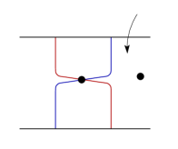
Figure 10: Positioning of the point $z$ and choice of $b_{i}$.

The point $z$ is placed outside the thin strips of isotopy between the $a_{i}$ and $b_{i}$. We denote by $x_{i}$ the unique intersection point between $a_{i}$ and $b_{i}$. Define

$$EH(P,\phi,\{a_{1},\dots,a_{n}\})=\{x_{1},\dots,x_{n}\}.$$

By construction of the Heegaard diagram $EH$ is a cycle in the Heegaard Floer homology associated to the data $(-\Sigma,\alpha,\beta,z)$. We choose the negative surface orientation since with this orientation there can be no holomorphic Whitney disc emanating from $EH$ (cf. Figure 10).

Lemma 8.15 (see [18]).

The Heegaard Floer cohomology $\widehat{\mbox{\rm HF}}\,^{\!*}(Y)$ is isomorphic to $\widehat{\mbox{\rm HF}}(-Y)$.

The Heegaard diagram $(-\Sigma,\alpha,\beta)$ is a Heegaard diagram for $-Y$ and, thus, represents the Heegaard Floer cohomology of $Y$. Instead of switching the surface orientation we can swap the boundary conditions of the Whitney discs at their $\alpha$-boundary and $\beta$-coundary, i.e. we will be interested in Whitney discs in $(\Sigma,\beta,\alpha)$. The element $EH$ can be interpreted as sitting in the Heegaard Floer cohomology of $Y$. The push-off $b_{i}$ is chosen such that there is no holomorphic disc emanating from $x_{i}$.

Theorem 8.16.

The class $EH(P,\phi,\{a_{1},\dots,a_{n}\})$ is independent of the choices made in its definition. Moreover, the associated cohomology class $c(Y,\xi)$ is an isotopy invariant of the contact structure $\xi$, up to sign. We call $c(Y,\xi)$ contact element.

The proof of this theorem relies on several steps we would like to sketch: An arc slide is a geometric move allowing us to change the cut system. Any two cut systems can be transformed into each other by a finite sequence of arc slides. Let $a_{1}$ and $a_{2}$ be two adjacent arcs. Adjacent means that in $P\backslash\{a_{1},\dots,a_{n}\}$ one of the boundary segments associated to $a_{1}$ and $a_{2}$ are connected via one segment $\tau$ of $\partial P$. An arc slide of $a_{1}$ over $a_{2}$ (or vice versa) is a curve in the isotopy class of $a_{1}\cup\tau\cup a_{2}$. We denote it by $a_{1}+a_{2}$.

Lemma 8.17.

Any two cut systems can be transformed into each other with a finite number of arc slides.

It is easy to observe that an arc slide affects the associated Heegaard diagram by two handle slides. The change under the $\alpha$-circles is given by a handle slide of $\alpha_{1}$ over $\alpha_{2}$. But the associated $\beta$-curve moves with the $\alpha$-curve, i.e. we have to additionally slide $\beta_{1}$ over $\beta_{2}$. We have to see that these handle slides preserve the contact element. To be more precise: After the first handle slide we moved out of the set of Heegaard diagrams induced by open books. Thus, we cannot see the contact element in that diagram. After the second handle slide, however, we move back into that set and, hence, see the contact element again. We have to check that the composition of the maps between the Heegaard Floer cohomologies induced by the handle slides preserves the contact element. This is a straightforward computation.

Definition 8.18.

Let a Heegaard diagram $(\Sigma,\alpha,\beta)$ and a homologically essential, simple, closed curve $\delta$ on $\Sigma$ be given. The Heegaard diagram $(\Sigma,\alpha,\beta)$ is called $\delta$-adapted if the following conditions hold.

1. It is induced by an open book and the pair $\alpha$, $\beta$ is induced by a cut system (cf. §8.3) for this open book.

2. The curve $\delta$ intersects $\beta_{1}$ once and does not intersect any other of the $\beta_{i}$, $i\geq 2$.

We can always find $\delta$-adapted Heegaard diagrams. This is already stated in [8] and [10] but not proved.

Lemma 8.19.

Let $(P,\phi)$ be an open book and $\delta\subset P$ a homologically essential closed curve. There is a choice of cut system on $P$ that induces a $\delta$-adapted Heegaard diagram.

Observe that $a_{1},\dots,a_{n}$ to be a cut system of a page $P$ essentially means to be a basis of $H_{1}(P,\partial P)$: Suppose the curves are not linearly independent. In this case we are able to identify a surface $F\subset P$, $F\not=P$, bounding a linear combination of some of the curves $a_{i}$. But this means the cut system disconnects the page $P$ in contradiction to the definition. Conversely, suppose the curves in the cut system are homologically linearly independent. In this case the curves cannot disconnect the page. If they disconnected, we could identify a surface $F$ in $P$ with boundary a linear combination of some of the $a_{i}$. But this contradicts their linear independence. The fact that $\Sigma\backslash\{a_{1},\dots,a_{n}\}$ is a disc shows that every element in $H_{1}(P,\partial P)$ can be written as a linear combination of the curves $a_{1},\dots,a_{n}$.

Proof.

Without loss of generality, we assume that $P$ has connected boundary: Suppose the boundary of $P$ has two components. Choose a properly embedded arc connecting both components of $\partial P$. Define this curve to be the first curve $a_{0}$ in a cut system. Cutting out this curve $a_{0}$, we obtain a surface with connected boundary. The curve $a_{0}$ determines two segments $S_{1}$ and $S_{2}$ in the connected boundary. We can continue using the construction process for connected binding we state below. We just have to check the boundary points of the curves to remain outside of the segments $S_{1}$ and $S_{2}$. Given that $P$ has more than two boundary components, we can, with this algorithm, inductively decrease the number of boundary components.
The map $\phi$ is an element of the mapping class group of $P$. Thus, if $\{a_{1},\dots,a_{n}\}$ is a cut system, then $\{\phi(a_{1}),\ldots,\phi(a_{n})\}$ is a cut system, too. It suffices to show that there is a cut system $\{a_{1},\ldots,a_{n}\}$ such that $\delta$ intersects $a_{i}$ once if and only if $i=1$.

2pt $\gamma$ [bl] at 199 214

Figure 11: Possible choice of curve $\gamma$.

We start by taking a band sum of $\delta$ with a small arc $\gamma$ as shown in Figure 11. We are free to choose the arc $\gamma$. Denote the result of the band sum by $a_{2}$. The arc $a_{2}$ indeed bounds a compressing disc in the respective handlebody because its boundary lies on $\partial P$. Because of our prior observation it suffices to show that $a_{2}$ is a primitive class in $H_{1}(P,\partial P)$. Since $H_{1}(P,\partial P)$ is torsion free the primitiveness of $a_{2}$ implies that we can extend $a_{2}$ to a basis of $H_{1}(P,\partial P)$. The curves defining this basis can easily be chosen to be not closed, with their boundary lying on $\partial P$.
Writing down the long exact sequence of the pair $(P,\partial P)$ we see that $\partial_{*}$ is surjective since $\partial_{*}[P]=[\partial P]$. Hence, exactness of the sequence implies that the inclusion $\iota\colon\thinspace P\longrightarrow(P,\partial P)$ induces an isomorphism on homology. Note that the zero at the end of the sequence appears because $\partial P$ is assumed to be connected. Let $g$ denote the genus of $P$. Of course $H_{1}(P;\mathbb{Z})$ is $\mathbb{Z}^{2g}$, which can be seen by a Mayer-Vietoris argument or from handle decompositions of surfaces (compute the homology using a handle decomposition). Since $\delta$ was embedded it follows from the lemma below that it is a primitive class in $H_{1}(P;\mathbb{Z})$. The isomorphism $\iota_{*}$ obviously sends $\delta$ to $a_{2}$, i.e. $\iota_{*}[\delta]=[\gamma]$. Thus, $a_{2}$ is primitive in $H_{1}(P,\partial P)$.

Cut open the surface along $\delta$. We obtain two new boundary components, $C_{1}$ and $C_{2}$ say, which we can connect with the boundary of $P$ with two arcs. These two arcs, in $P$, determine a properly embedded curve, $a_{1}$ say, whose boundary lies on $\partial P$. Furthermore, $a_{1}$ intersects $\delta$ in one single point, transversely. The curve $a_{1}$ is primitve, too. To see, that we can extend to a cut system such that $\delta$ is disjoint from $a_{3},\dots,a_{n}$, cut open the surface $P$ along $\delta$ and $a_{1}$. We obtain a surface $P^{\prime}$ with one boundary component. The curves $\delta$ and $a_{1}$ determine $4$ segments, $S_{1},\dots,S_{4}$ say, in this boundary. We extend $a_{2}$ to a cut system $a_{2},\dots,a_{n}$ of $P^{\prime}$ and arrange the boundary points of the curves $a_{3},\dots,a_{n}$ to be disjoint from $S_{1},\dots,S_{4}$. The set $a_{1},\dots,a_{n}$ is a cut system of $P$ with the desired properties. ∎

As a consequence of the proof we may arrange $\delta$ to be a push-off of $a_{2}$ outside a small neighborhood where the band sum is performed. Geometrically spoken, we cut open $\delta$ at one point, and move the boundaries to $\partial P$ to get $a_{2}$. Given a positive Giroux stabilization, we can find a special cut system which is adapted to the curve $\gamma$. It is not hard to see that there is only one homotopy class of triangles that connect the old with the new contact element and that the associated moduli space is a one-point space.

Lemma 8.20.

An embedded circle $\delta$ in an orientable, compact surface $\Sigma$ which is homologically essential is a primitive class of $H_{1}(\Sigma,\mathbb{Z})$.

Proof.

Cut open the surface $\Sigma$ along $\delta$. We obtain a connected surface $S$ with two boundary components since $\delta$ is homologically essential in $\Sigma$. We can recover the surface $\Sigma$ by connecting both boundary components of $S$ with a $1$-handle and then capping off with a disc. There is a knot $K\subset S\cup h^{1}$ intersecting the co-core of $h^{1}$ only once and intersecting $\delta$ only once, too. To construct this knot take a union of two arcs in $S\cup h^{1}$ in the following way: Namely, define $a$ as the core of $h^{1}$, i.e. as $D^{1}\times\{0\}\subset D^{1}\times D^{1}\cong h^{1}$ and let $b$ be a curve in $S$, connecting the two components of the attaching sphere $h^{1}$ in $\partial S$. We define $K$ to be $a\cup b$. Obviously,

$$\pm 1=\#(K,\delta)=\bigl{<}PD[K],[\delta]\bigr{>}.$$

Since $H_{1}(\Sigma;\mathbb{Z})$ is torsion, free $H^{1}(\Sigma;\mathbb{Z})\cong\mbox{\rm Hom}(H_{1}(\Sigma;\mathbb{Z}),\mathbb{Z})$. Thus, $[\delta]$ is primitive. ∎

Recall that a positive/negative Giroux stabilization of an open book $(P,\phi)$ is defined as the open book $(P^{\prime},D^{\pm}_{\gamma}\circ\phi)$ where $P^{\prime}$ is defined by attaching a $1$-handle to $P$ and $\gamma$ is a embedded, simple closed curve in $P^{\prime}$ that intersects the co-core of $h^{1}$ once (see Definition 8.10). Using the proofs of Lemma 8.11 and Lemma 8.12, we see that there is a cut system $\{a_{1},\dots,a_{n+1}\}$ of the stabilized open book such that $\gamma$ intersects only $a_{n+1}$ which is the co-core of $h^{1}$. Denote by $\alpha=\{\alpha_{1},\dots,\alpha_{n}\}$ the associated attaching circles. We define a map

$$\Phi\colon\thinspace\widehat{\mbox{\rm CF}}(\Sigma,\alpha,\beta,z)\longrightarrow\widehat{\mbox{\rm CF}}(\Sigma\#T^{2},\alpha\cup\{\alpha_{n+1}\},\beta\cup\{\beta_{n+1}\},z)$$

by assigning to $x\in\mathbb{T}_{\alpha}\cap\mathbb{T}_{\beta}$ the element $\Phi(x)=(x,q)$ where $q$ is the unique intersection point $\gamma\cap a_{n+1}$. This is an isomorphism by reasons similar to those given in Example 4.1.
With our preparations done, we can easily prove one of the most significant properties of the contact element: Its functoriality under $(+1)$-contact surgeries. We will outline the proof since it can be regarded as a model proof.

Theorem 8.21 ([15]).

Let $(Y^{\prime},\xi^{\prime})$ be obtained from $(Y,\xi)$ by $(+1$)-contact surgery along a Legendrian knot $L$. Denote by $W$ the associated cobordism. Then the map

$$\widehat{F}_{-W}\colon\thinspace\widehat{\mbox{\rm HF}}(-Y)\longrightarrow\widehat{\mbox{\rm HF}}(-Y^{\prime})$$

preserves the contact element, i.e. $\widehat{F}_{-W}(c(Y,\xi))=c(Y^{\prime},\xi^{\prime})$.

Proof.

2pt $x^{\prime}_{1}$ [B] at 149 230 $z$ [r] at 201 239 $\mathcal{D}_{z}$ [l] at 255 242 $\gamma_{1}$ [B] at 272 167 $\beta_{1}$ [t] at 12 129 $\widehat{\Theta}_{1}$ [t] at 97 129 $x_{1}$ [t] at 147 73 $\alpha_{1}$ [t] at 283 97 Domain of a holomorphic triangle [t] at 133 23 ₁ [t] at 38 208 ₂ [l] at 70 236

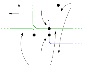
Figure 12: Significant part of the Heegaard triple diagram.

Let an open book $(P,\phi)$ adapted to $(Y,\xi,L)$ be given. By Lemma 8.14, a $(+1)$-contact surgery acts on the monodromy as a composition with a negative Dehn twist. Without loss of generality, the knot $L$ just intersects $\beta_{1}$ once, transversely and is disjoint from the other $\beta$-circles. Moreover, we can arrange the associated Heegaard triple to look as indicated in Figure 12. The contact element $c(Y,\xi)$ is represented by the point $\{x_{1},\dots,x_{n}\}$. Obviously, there is only one domain which carries a holomorphic triangle. It is the small holomorphic triangle connecting $x_{1}$ and $x_{1}^{\prime}$ (cf. §4.4). Thus, there is only one domain with positive coefficients, with $n_{z}=0$, connecting the points $\{x_{1},\dots,x_{n}\}$ with $\{x_{1}^{\prime},\dots,x_{n}^{\prime}\}$. By considerations similar to those given at the end of the proof of Lemma 4.9, we see that the associated moduli space is a one-point space. Hence, the result follows. ∎

8.5 The Invariant $\widehat{\mathcal{L}}$

Ideas very similar to those used to define the contact element can be utilized to define an invariant of Legendrian knots we will briefly call LOSS. This invariant is due to Lisca, Ozsváth, Stipsicz and Szabó and was defined in [10]. It is basically the contact element but now it is interpreted as sitting in a filtered Heegaard Floer complex. The filtration is constructed with respect to a fixed Legendrian knot:

2pt Page $P\!\times\!\{1/2\}$ of the open book [bl] at 131 189 $w$ [l] at 95 116 $z$ [b] at 167 104 $w$ [tl] at 332 53 $z$ [t] at 408 85

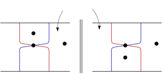
Figure 13: Positioning of the point $w$ depending on the knot orientation.

Let $(Y,\xi)$ be a contact manifold and $L\subset Y$ a Legendrian knot. There is an open book decomposition of $Y$, subordinate to $\xi$, such that $L$ sits on the page $P\times\{1/2\}$ of the open book (cf. §8.3). Choose a cut system that induces an $L$-adapted Heegaard diagram (cf. §8.4, Definition 8.18 and Lemma 8.19). Figure 13 illustrates the positioning of a point $w$ in the Heegaard diagram induced by the open book. Similar to the case of the contact element those intersection points $\alpha_{i}\cap\beta_{i}$ who sit on $P\times\{1/2\}$ determine one specific generator of $\widehat{\mbox{\rm CF}}(-Y)$. This element may be interpreted as sitting in $\widehat{\mbox{\rm CFK}}(-Y,L)$, and it is a cycle there, too. The induced element in the knot Floer homology is denoted by $\widehat{\mathcal{L}}(L)$.

Remark.

1. Since this is an important issue we would like to recall the relation between the pair $(w,z)$ and the knot orientation. In homology we connect $z$ with $w$ in the complement of the $\alpha$-curves and $w$ with $z$ in the complement of the $\beta$-curves (oriented as is obvious from the definition). In cohomology we orient in the opposite manner, i.e. we move from $z$ to $w$ in the complement of the $\beta$-curves and from $w$ to $z$ in the complement of the $\alpha$-curves.

2. Observe, that the definition of the invariant $\widehat{\mathcal{L}}$ as well as the contact element always comes with a specific presentation of the groups $\widehat{\mbox{\rm HF}}$ and $\widehat{\mbox{\rm HFK}}$. If we want to compare for instance invariants of two different Legendrian knots, we have to get rid of the presentation in the background. This can be done by modding out a certain mapping class group action on the homologies. We point the reader to [13].

Analogous to the properties of the contact element the invariant $\widehat{\mathcal{L}}$ is preserved when a $(+1)$-contact surgery is performed in its complement (see [13]): Suppose we are given a contact manifold $(Y,\xi)$ with two Legendrian knots $L$ and $S$ sitting in it. Performing a $(+1)$-contact surgery along $S$, denote by $W$ the associated cobordism. Furthermore, we denote by $(Y_{S},\xi_{S})$ the result of the contact surgery. The cobordism $-W$ induces a map

$$\widehat{F}_{-W}\colon\thinspace\widehat{\mbox{\rm HFK}}(-Y,L)\longrightarrow\widehat{\mbox{\rm HFK}}(-Y_{S},L_{S})$$

such that $\widehat{F}_{-W}(\widehat{\mathcal{L}}(L))=\widehat{\mathcal{L}}(L_{S})$. Here, $L_{S}$ denotes the knot $L$ in the manifold $Y_{S}$. Observe, that the cobordism maps constructed for the hat-theory can be defined the same way for knot Floer homologies.

Finally, the contact element and the invariant $\widehat{\mathcal{L}}$ are connected, too. Performing a $(+1)$-contact surgery along the knot $L$, denote by $W$ the associated cobordism and by $(Y_{L},\xi_{L})$ the result of the contact surgery. The cobordism $-W$ induces a map

$$\Gamma_{-W}\colon\thinspace\widehat{\mbox{\rm HFK}}(-Y,L)\longrightarrow\widehat{\mbox{\rm HF}}(-Y_{L}^{+})$$

such that $\Gamma_{-W}(\widehat{\mathcal{L}}(L))=c(\xi_{L}^{+})$ (see [26]). This map is not defined by counting holomorphic triangles. It needs a specific construction we do not outline here. We point the interested reader to [26].

References

- [1] G. E. Bredon, Geometry and Topology, Graduate Texts in Mathematics, Vol. 139, Springer-Verlag, 1993.
- [2] F. Ding and H. Geiges, Symplectic fillability of tight contact structures on torus bundles, Algebr. Geom. Topol. 1 (2001), 153–172.
- [3] F. Ding and H. Geiges, A Legendrian surgery presentation of contact -manifolds, Math. Proc. Cambridge Philos. Soc. 136 (2004), 583–598.
- [4] Y. Eliashberg, Topological characterization of Stein manifolds of dimension , Internat. J. Math. 1 (1990), 29–46.
- [5] J. B. Etnyre, Lectures on open-book decompositions and contact structures, Amer. Math. Soc. 5 (2006), 103–142, (Proceedings of the Clay Mathematics Summer School).
- [6] H. Geiges, An Introduction to Contact Topology, Cambridge Studies in Advanced Mathematics, Vol. 109, Cambridge University Press, 2008.
- [7] R. E. Gompf and A. I. Stipsicz, -Manifolds and Kirby Calculus, Graduate Studies in Mathematics, Vol. 20, American Mathematical Society, 1999.
- [8] K. Honda, W. H. Kazez, and G. Matić, On the contact class in Heegaard Floer homology, J. Diff. Geom., to appear.
- [9] R. Lipshitz and P. Ozsváth and D. Thurston, Bordered Heegaard Floer homology: Invariance and pairing, arXiv:0810.0687.
- [10] P. Lisca, P. Ozsváth, A. I. Stipsicz, and Z. Szabó, Heegaard Floer invariants of Legendrian knots in contact three-manifolds, JEMS, to appear.
- [11] D. McDuff and D. Salamon, -Holomorphic Curves and Symplectic Topology, Colloquium Publications, Vol. 52, American Mathematical Society, 2004.
- [12] A. Juhasz, Holomorphic disks and sutured manifolds, Algebr. Geom. Topol. 6 (2006), 1429–1457.
- [13] P. Ozsváth and A. I. Stipsicz, Contact surgeries and the transverse invariant in knot Floer homology, arXiv:0803.1252.
- [14] P. Ozsváth and Z. Szabó, Holomorphic disks and knot invariants, Adv. Math. 186(1) (2004), 58–116.
- [15] P. Ozsváth and Z. Szabó, Heegaard Floer homologies and contact structures, Duke Math. J. 129(1) (2005), 39–61.
- [16] P. Ozsváth and Z. Szabó, Heegaard diagrams and holomorphic disks, Diff. faces of Geom., Int. Math. Series, 301–348.
- [17] P. Ozsváth and Z. Szabó, Holomorphic disks and topological invariants for closed three-manifolds, Ann. of Math. 159(3) (2004), 1027–1158.
- [18] P. Ozsváth and Z. Szabó, Holomorphic disks and three-manifold invariants: Properties and applications, Ann. of Math. 159(3) (2004), 1159–1245.
- [19] P. Ozsváth and Z. Szabó, Holomorphic triangles and invariants of smooth four-manifolds, Adv. Math. 202(2) (2006), 326–400.
- [20] P. Ozsváth and Z. Szabó, On the Heegaard Floer homology of branched double-covers, Adv. in Math. 194 (2005), 1–33.
- [21] P. Ozsváth and Z. Szabó, Introduction to Heegaard Floer theory, Clay Math. Proc. Volume 5 (2006), 3-28.
- [22] P. Ozsváth and Z. Szabó, Lectures on Heegaard Floer homology, Clay Math. Proc. Volume 5 (2006), 29-70.
- [23] P. Ozsváth and Z. Szabó, Heegaard diagrams and holomorphic disks, arXiv:math/0403029.
- [24] P. Ozsváth and Z. Szabó, On the skein exact sequence for knot Floer homology, arXiv:0707.1165.
- [25] B. Ozbagci and A. I. Stipsicz, Surgery on Contact -Manifolds and Stein Surfaces, Bolyai Society Mathematical Studies Volume 13, Springer-Verlag, 2004.
- [26] B. Sahamie, Dehn twists in Heegaard Floer homology, Algebr. Geom. Topol. 10(1) (2010), 465–524.
- [27] S. Sarkar and J. Wang, An algorithm for computing some Heegaard Floer homologies, (2008), to appear in Ann. of Math.
- [28] V. Turaev, Torsion invariants of -structures on -manifolds, Math. Research Letters 6 (1997), 679–695.