The Modulation of de Haas-van Alphen Effect in Graphene by Electric Field

Abstract

This paper is to explore the de Haas-van Alphen effect $(dHvA)$ of graphene in the presence of an in-plane uniform electric field. Three major findings are yielded. First of all, the electric field is found to modulate the de Haas-van Alphen magnetization and magnetic susceptibility through the dimensionless parameter $(\beta=\frac{E}{\upsilon_{F}B})$. As the parameter $\beta$ increases, the values of magnetization and magnetic susceptibility increase to positive infinity or decrease to negative infinity at the exotic point $\beta_{c}=1$. Besides, the $dHvA$ oscillation amplitude rises abruptly to infinity for zero temperature at $\beta_{c}=1$, but eventually collapses at a finite temperature thereby leading to the vanishing of de Haas-van Alphen effect. In addition, the magnetic susceptibility depends on the electric and magnetic fields, suggesting that the graphene should be a non-linear magnetic medium in the presence of the external field. These results, which are different from those obtained in the standard nonrelativistic 2D electron gas, are attributed to its anomalous Landau level spectrum in graphene.

1 Introduction

Owing to the progress of experimental methods, graphene (or a graphite monolayer) is now gaining increasing interests in the field of physics of electronic systems with reduced dimensionality [1, 2, 3, 4]. It is promising to be applied in nanoelectronics because of the exotic chiral features [5, 6, 7, 8, 9] in its electronic structure. In particular, such two-dimensional (2D) or quasi-two-dimensional systems have led to some of the most startling discoveries in condensed matter physics in the recent years. Moreover, these anomalous phenomena are found to be tied to the remarkable ”relativistic-like” spectrum of electrons and holes in graphene, which makes graphene important and interesting in physics. One of them that have been experimentally testified is the abnormality of the 2D quantum Hall effect [10, 11].

Another important physics effect is the de Haas-van Alphen $(dHvA)$ oscillation of the graphene. It has been predicted in Ref. [12], which proposes that the magnetization oscillates periodically in a sawtooth pattern as a function of $1/B$, in agreement with the old Peierls prediction [13]. A question of great interest arising here is what will happen if an additional electric field is applied in graphene. Indeed, the electric and magnetic fields effects on its magnetization and magnetic susceptibility are of vital significance to our understanding of the Dirac fermion behaviors. However, little theoretical or experimental research has been done on this issue yet.

Motivated by the concerns mentioned above, the present study is to investigate the 2D $dHvA$ effect of the graphene in the presence of the electric field. The paper is organized as follows. In section $2$, a brief introduction is given to the 2D model for graphene. The energy eigenvalues and eigenstates, as well as the density of states $(DOS)$ and the $dHvA$ oscillation period $\Delta(1/B)$ are obtained analytically. Section $3$ describes some details of the magnetization and magnetic susceptibility study. In the meantime, the analytical expressions are derived for the magnetization and magnetic susceptibility. More specifically, the one regarding the condition of $T=0~{}\mbox{K}$ is reported in section $3.1$ while the one pertaining to the condition of nonzero temperature in section $3.2$. The section winds up with a discussion of the modulation of $dHvA$ in graphene by the electric field. In the last section, the conclusions are presented.

2 Energy eigenvalues and eigenstates

In order to investigate the modulation of $dHvA$, we begin with the study of the energy eigenvalues and eigenstates belonging to the carriers in graphene. The charge carriers in graphene mimic relativistic particles with zero rest mass and have an effective ‘speed of light’ $c^{\ast}=\upsilon_{F}\thickapprox 1.0\times 10^{6}$ ms^-1, which is essentially governed by Dirac equation [10, 11]. So we start by considering the Dirac equation for such a 2D gas of Dirac fermions in crossed electric $\left[\vec{E}=\left(-E,0,0\right),U=Eex\right]$ and magnetic $\left[\vec{B}=\left(0,0,B\right),\vec{A}=\left(0,Bx,0\right)\right]$ fields, where $E$ is the electric field strength and $B$ the magnetic induction intensity. The single particle Hamiltonian is then given by

$$\hat{H}=\upsilon_{F}\mathbf{\hat{\alpha}\cdot\Pi}+\mathbf{\hat{I}}eEx$$ (1)

in which $\hat{\alpha}$ is the Pauli matrix, $\Pi$ is the canonical momentum, $\hat{I}$ is the 2 $\times$ 2 unit matrix. Following Landau and Lifshitz [14] the first-order equation of eigenvalue problem of $\hat{H}$ becomes the second-order equation

$$\left[\left(\varepsilon-eEx\right)^{2}-\left(\upsilon_{F}\vec{p}-e\vec{A}\right)^{2}+e\hbar B\upsilon_{F}^{2}\mathbf{\hat{\alpha}}_{z}+ie\hbar E\upsilon_{F}\mathbf{\hat{\alpha}}_{x}\right]\Psi=0,$$ (2)

where $\varepsilon$ is the eigenvalue of $\hat{H}$ and other notations are standard. From Eq. (2), we obtain the energy spectra and eigenfunctions of the problem,

$$\varepsilon_{n,k_{y}}=sgn\left(n\right)\sqrt{2\left|n\right|\hbar eB}\upsilon_{F}\left(1-\beta^{2}\right)^{3/4}+\hbar\upsilon_{F}\beta k_{y},$$ (3)

$$\Psi_{n,k_{y}}(x,y)\propto\exp\left(ik_{y}y\right)\exp[-(\beta/2)\alpha_{y}]\left({}_{i^{\left|n\right|}\phi_{n}\left(\xi\right)}^{sgn(n)i^{\left|n\right|-1}\phi_{\left|n\right|-1}\left(\xi\right)}\right),$$ (4)

with

$$\xi\equiv\frac{\left(1-\beta^{2}\right)^{1/4}}{l_{c}}\left(x+l_{c}^{2}k_{y}-sgn(n)\frac{\sqrt{2\left|n\right|}l_{c}\beta}{(1-\beta^{2})^{1/4}}\right).$$ (5)

In Eq. (3), $e$ and $\hbar=h/2\pi$ are electron charge and Planck’s constant divided by $2\pi$, respectively. The integer $n$ represents the Landau level index, $k_{y}=2\pi l/L_{y}$ $\left(l=0,\pm 1,\pm 2,\cdot\cdot\cdot,\right)$ is the quantum number corresponding to the translation symmetry along the $y$ axis, $L_{y}$ stands for the size of the graphene in $y$ direction. The electric field dependent dimensionless parameter $\beta$ is defined by $\beta=E/\left(\upsilon_{F}B\right)$ and obeys $\left|\beta\right|<1$, where $\upsilon_{F}$ is the Fermi velocity. In Eq. (4), $\phi_{n}\left(\xi\right)$ are the harmonic oscillator eigenfunctions. From Eq. $(5)$ we observe that the centers of the x-dependent orbits are located at

$$x_{0}=l_{c}^{2}k_{y}-sgn(n)\frac{\sqrt{2\left|n\right|}l_{c}\beta}{(1-\beta^{2})^{1/4}}$$ (6)

where $l_{c}=\sqrt{\hbar/eB}$ is the magnetic length. The eigenvalues of $\hat{H}$ show that the exact energies are given by the sum of quantized harmonic-oscillator energies and the potential energy of a charged particle located at coordinate $x_{0}$ in potential field $U(x)$. They agree with those in Ref. [15], the authors of which solved the problem by transforming the original system into a case with the null electric field, in terms of a Lorentz boost transformation.

We then count the Landau states $\Psi_{n,k_{y}}$ in the presence of the potential $U(x)$ following the same argument employed in the absence of crossed electric field. Since $k_{y}=2\pi l/L_{y}$, the separation between adjacent allowed $k_{y}$ values is given by $\delta k_{y}=2\pi/L_{y}$. From Eq. (6) we may relate the possible range $\Delta k_{y}$ of $k_{y}$ to the physically accessible range $\Delta x_{0}$ of $x_{0}$:

$$\Delta x_{0}=l_{c}^{2}\Delta k_{y}.$$ (7)

Since $\Delta x_{0}=L_{x}$, in order for the Landau states to be centered within the strip $0\leq x_{0}\leq L_{x}$ we must have allowed the range of $k_{y}$ values given by $\Delta k_{y}=\Delta x_{0}/l_{c}^{2}.$ The number of Landau states $\Psi_{n,k_{y}}\left(x,y\right)$ per unit area for each quantum number $n$ is:

$$D_{n}=\frac{g_{s}\Delta k_{y}}{L_{x}L_{y}\delta k_{y}}=\frac{2eB}{\hbar\pi},$$ (8)

which is independent of $n$ and the degeneracy yields $g_{s}=4$, accounting for spin degeneracy and sublattice degeneracy in graphene.

We consider a system of $N$ electrons within an area $S$ moving in the potential $U(x)$ and the magnetic field $B$. Let the system remain at $0$ K and accordingly the free energy reduces to the total energy. The full occupation of Landau levels obeys $D_{n}S=N/\left(n_{F}+1\right)$ with Fermi quantum number $n_{F}$. The total energy $E=\sum_{n,k_{y}}\varepsilon_{n,k_{y}}\left(B\right)$ will give a discontinuous derivative $M=-\partial E/\partial B$ at the field values $B_{n}$ where $M$ is the magnetization. From $D_{n}S=N/\left(n_{F}+1\right)$ these discontinuities in the magnetization occur at reciprocal fields $1/B_{n}$, so that the period of magnetization oscillation is given by:

$$\Delta\left(\frac{1}{B}\right)=\frac{1}{B_{n+1}}-\frac{1}{B_{n}}=\frac{2e}{\pi\hbar N_{0}},$$ (9)

where $B_{n+1}$ and $B_{n}$ are the magnetic induction intensity corresponding to two neighboring levels, which cross the Fermi level in succession and $N_{0}=N/S$ is the sheet concentration. Eq. (9) means that the discontinuous zero-temperature oscillations are periodic in $1/B$. It is just compatible with the results regarding the null electric field obtained by Sharapov et al [12].

3 Magnetization and magnetic susceptibility

3.1 Zero temperature

Then we move on to investigate the magnetization of electrons in graphene in the presence of crossed uniform electric and magnetic fields at $T=0~{}\mbox{K}$. For simplicity, we ignore spin-orbit coupling of electrons in the present work. The magnetization reads [16, 17]

$$M=-\left(\partial E/\partial B\right)_{N}$$ (10)

where $E$ is the total energy and $N$ denotes the total number of electrons in graphene. To have units in Tesla, we symbolize $B=\mu_{p0}H$, $\mu_{p0}$ as being the magnetic permeability of free space, $H$ stands for the magnetic field intensity.

The total energy is given by:

$$E=\sum_{n,k_{y}}\varepsilon_{n,k_{y}} = \sum_{n=0}^{\left[\mu_{0}^{2}/2e\hbar\upsilon_{F}^{2}B\right]}D_{n}\left(\varepsilon_{n}-\mu\right)+\mu N_{0}$$ (11)

$$+\sum_{l=-l_{F}}^{l_{y}}\frac{2\pi}{L_{y}}\hbar\upsilon_{F}\beta l,\left(-l_{F}\leq l_{y}\leq l_{F}\right)$$

in which the last term is the additional energy induced by the electric field corresponding to the $n_{F}$th level partly occupied by electrons and we refer to it as $E_{add}$. Here $\varepsilon_{n}$ is defined as $\varepsilon_{n}=\sqrt{2n\hbar eB}\upsilon_{F}\left(1-\beta^{2}\right)^{3/4}$. The chemical potential $\mu=\mu_{0}\left(1-\beta^{2}\right)^{3/4}$ is derived analytically where $\mu_{0}$ refers to the zero-temperature chemical potential (equal to the Fermi energy) in the absence of electric and magnetic fields as expressed by $\mu_{0}=\hbar\upsilon_{F}\sqrt{N_{0}\pi}$. Using the formula for the generalized zeta function [18], $\zeta\left(z,\upsilon+k\right)=\zeta\left(z,\upsilon\right)-\sum_{m=0}^{k-1}\left(m+\upsilon\right)^{-z}$ and $\zeta\left(-1/2,0\right)\equiv\zeta\left(-1/2\right)\equiv-\left(1/4\pi\right)\zeta\left(3/2\right)$, one can write the first and the second terms in Eq. $(11)$ as the summation of the regular term,

$$E_{reg}=-\frac{\zeta\left(3/2\right)\upsilon_{F}}{\pi^{2}\sqrt{2\hbar}}\left(eB\right)^{3/2}\left(1-\beta^{2}\right)^{3/4}+\frac{2\mu_{0}^{3}}{3\pi\left(\hbar\upsilon_{F}\right)^{2}}\left(1-\beta^{2}\right)^{3/4},$$ (12)

and the oscillating term

$$E_{osc} = -\frac{2\sqrt{2\hbar}\upsilon_{F}}{\pi\hbar}\left(eB\right)^{3/2}\left(1-\beta^{2}\right)^{3/4}\zeta\left(-\frac{1}{2},1+\left[\frac{\mu_{0}^{2}}{2e\hbar\upsilon_{F}^{2}B}\right]\right)$$

$$-\left(1-\beta^{2}\right)^{3/4}\left[\frac{2\mu_{0}^{3}}{3\pi\left(\hbar\upsilon_{F}\right)^{2}}-\frac{2\mu_{0}eB}{\pi\hbar}\left(mod\left[\frac{\mu_{0}^{2}}{2e\hbar\upsilon_{F}^{2}B}\right]-\frac{1}{2}\right)\right].$$

In this expression, $\left[\mu_{0}^{2}/2e\hbar\upsilon_{F}^{2}B\right]$ stands for the integer part of $\mu_{0}^{2}/2e\hbar\upsilon_{F}^{2}B$ and the mod $\left[\mu_{0}^{2}/2e\hbar\upsilon_{F}^{2}B\right]$ is the fractional part of $\mu_{0}^{2}/2e\hbar\upsilon_{F}^{2}B$.

Making use of $\Gamma$ function $\Gamma\left(n+\alpha\right)=\int_{0}^{\infty}dss^{n+\alpha-1}e^{-s}$ and Bernoulli polynomials $B_{n}\left(y\right)$, $\sum_{n=0}^{\infty}\frac{x^{n}}{n!}B_{n}\left(y\right)=\frac{xe^{xy}}{e^{x}-1},$ $\left(\left|x\right|<2\pi\right),$ we obtain

$$\sum_{n=2}^{\infty}\frac{\Gamma\left(n+\alpha\right)B_{n}\left(y\right)}{n!}x^{n}$$ (14)

$$= \int_{0}^{\infty}dss^{\alpha-1}e^{-s}\left[\frac{sxe^{sxy}}{e^{sx}-1}-1-sxB_{1}\left(y\right)\right],$$

where the explicit expressions for the Bernoulli polynomials $B_{0},B_{1},B_{2}$ are

$$B_{0}\left(y\right)=1,B_{1}\left(y\right)=y-1/2,B_{2}\left(y\right)=y^{2}-y-1/6.$$ (15)

The Bernoulli polynomials depend on $mod\left[y\right]$ in the following equations, i.e. $B_{n}\left(mod\left[y\right]\right).$ For brevity, we write it as $B_{n}\left(y\right)$.

Using the formula [17]

$$\int_{0}^{\infty}\frac{x^{v-1}e^{-\mu x}dx}{1-e^{-\beta x}}=\frac{1}{\beta^{v}}\Gamma\left(v\right)\zeta\left(v,\frac{\mu}{\beta}\right),\left(Re\mu>0,Rev>0\right)$$

we have

$$E_{osc}=\frac{2\left(eB\upsilon_{F}\right)^{2}}{\pi^{3/2}\mu_{0}}\left(1-\beta^{2}\right)^{3/4}\sum_{n=0}^{\infty}\frac{\Gamma\left(n+1/2\right)B_{n+2}\left(w/2\right)}{\left(n+2\right)!}\left(\frac{2e\hbar\upsilon_{F}^{2}B}{\mu_{0}^{2}}\right)^{n}$$

in which $w=\mu_{0}^{2}/\left(e\hbar\upsilon_{F}^{2}B\right)$. Regarding small fields, $eB\hbar\upsilon_{F}^{2}\ll\mu_{0}^{2}$, we can apply the following asymptotic expansions for $J_{1}=\int_{0}^{\infty}dte^{-tp}/\left[\sqrt{\pi t}\left(t^{2}+1\right)\right]$:

$$J_{1}\left(p\right)=\frac{1}{\sqrt{\pi}}\sum_{n=0}^{\infty}\frac{\left(-1\right)^{n}\Gamma\left(n+1/2\right)}{p^{n+1/2}}$$ (17)

and the Bernoulli polynomials $B_{n}$ periodically continue beyond the interval [0,1]:

$$B_{n} = -\frac{2n!}{\left(2\pi\right)^{n}}\sum_{k=1}^{\infty}\frac{1}{k^{n}}\cos\left(2\pi kx-\frac{n\pi}{2}\right),$$ (18)

$$n > 1,0\leq x\leq 1;n=1,0<x<1.$$

It is easy to get the following form:

$$E_{osc}=\frac{\left(eB\right)^{3/2}\upsilon_{F}}{\sqrt{\hbar}\pi}\left(1-\beta^{2}\right)^{3/4}\sum_{k=1}^{\infty}\frac{1}{\left(\pi k\right)^{3/2}}J_{1}\left(\pi kw\right)\cos\left(\pi kw\right).$$ (19)

For $\sqrt{eB\hbar\upsilon_{F}^{2}}\ll\mu_{0}$, keeping the leading term in asymptotic expansions for $J_{1}\left(p\right)$, we finally obtain from Eq. (19)

$$E_{osc}\cong\frac{\left(eB\upsilon_{F}\right)^{2}}{\pi\mu_{0}}\left(1-\beta^{2}\right)^{3/4}\sum_{k=1}^{\infty}\frac{\cos\left(\pi kw\right)}{\left(\pi k\right)^{2}}.$$ (20)

Hence the total energy $E$ can be expressed as a sum of regular, oscillating and the additional energy terms,

$$E=E_{reg}+E_{osc}+E_{add}.$$ (21)

According to the results reported above, we get the corresponding de Haas-van Alphen magnetization,

$$M_{reg}=\frac{3e\sqrt{eB\hbar}\varsigma\left(3/2\right)\upsilon_{F}}{2\sqrt{2}\pi^{2}\hbar\left(1-\beta^{2}\right)^{1/4}}-\frac{\mu_{0}^{3}\beta^{2}}{\pi\left(\hbar\upsilon_{F}\right)^{2}B\left(1-\beta^{2}\right)^{1/4}},$$ (22)

$$M_{add}=\frac{\pi\hbar\upsilon_{F}\beta}{BL_{y}}A_{M_{0}},$$ (23)

where

$$A_{M_{0}}=\left[\frac{\mu_{0}^{4}}{\pi^{2}\left(\hbar\upsilon_{F}\right)^{4}}-\left[\frac{\mu_{0}^{2}}{2e\hbar\upsilon_{F}^{2}B}\right]\left(\left[\frac{\mu_{0}^{2}}{2e\hbar\upsilon_{F}^{2}B}\right]+1\right)\left(\frac{2eB}{\hbar\pi}\right)^{2}\right].$$ (24)

This expression involves a dependence on the integer part $\left[\mu_{0}^{2}/2e\hbar\upsilon_{F}^{2}B\right]$ and

$$M_{osc}=A_{M1}\sum_{k=1}^{\infty}\frac{(-1)^{k}}{\pi k}\sin\left(\frac{\pi k\mu_{0}^{2}}{e\hbar\upsilon_{F}^{2}B}\right)+A_{M2}\sum_{k=1}^{\infty}\frac{(-1)^{k}}{\left(\pi k\right)^{2}}\cos\left(\frac{\pi k\mu_{0}^{2}}{e\hbar\upsilon_{F}^{2}B}\right),$$

where $A_{M1}=-\frac{e\mu_{0}\left(1-\beta^{2}\right)^{3/4}}{\pi\hbar}$ and $A_{M2}=-\frac{\left(e\upsilon_{F}\right)^{2}B\left(4-\beta^{2}\right)}{2\pi\mu_{0}\left(1-\beta^{2}\right)^{1/4}}$.

Figure 1 shows that the $dHvA$ oscillation on the magnetization $M$ modulated by electric field in graphene. As shown in Fig. 1(a), the magnetization $M$ oscillates periodically in $1/B$ with the period of $\Delta\left(1/B\right)=2e\hbar\upsilon_{F}^{2}/\mu_{0}^{2}$. Three oscillation curves correspond to the applied electric field strength $E_{1}=5$ V/m, $E_{2}=10$ V/m and $E_{3}=15$ V/m, respectively. From these curves, one can see that the oscillation amplitude $(OA)$ of magnetization is proportional to the electric field $E$. Also, the $OA$ ascends significantly with increasing $1/B$, but remains unchanged for the null electric field in Ref. [12]. Thus, it is demonstrated the electric field effect on the $OA$ of magnetization. However unexpected it may be, according to Eq. (3.1) the $OA$ increases abruptly to infinity at $\beta_{c}=1$ thereby leading to the vanishing of $dHvA$ oscillation. It is interesting that the abnormal phenomena will die out if the electric filed vanishes. Thus, it can be also attributed to the electric field effect. We hope that the new findings will be verified when magnetization experiments under in-plane electric field are carried out in graphene. The predicted effect will hopefully also help interpretation of magnetization in experiment.

Meanwhile, we find that these peculiar features are absent in standard quantum 2D electron gas systems [19, 20, 21]. Hence, the possible reason for the effect might be that it is determined by the ”relativistic” character of carriers in graphene, unlike the usual sample, which can be traced to the exotic structure in graphene.

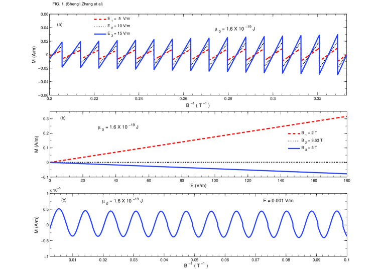
Figure 1: $\left(a\right)$ Magnetization $M$ is plotted as a function of reciprocal magnetic field $1/B$ for a given chemical potential $\mu_{0}=1.6\times 10^{-19}~{}\mbox{J}$ and $T=0~{}\mbox{K}$. Three oscillation curves correspond to $E_{1}=5~{}\mbox{V/m}$, $E_{2}=10~{}\mbox{V/m}$ and $E_{3}=15~{}\mbox{V/m}$, respectively. $\left(b\right)$ $M$ plotted vs electric field $E$ for $\mu_{0}=1.6\times 10^{-19}~{}\mbox{J}$ and $T=0~{}\mbox{K}$. Three curves correspond to $B_{1}=2~{}\mbox{T}$, $B_{2}=3.63~{}\mbox{T}$ and $B_{3}=5~{}\mbox{T}$, respectively. $\left(c\right)$ The magnetization, $M$, as a function of $1/B$ at $E=0.001~{}\mbox{V/m}$, $\mu_{0}=1.6\times 10^{-19}~{}\mbox{J}$ and $T=0~{}\mbox{K}$.

Figure 1(b) demonstrates that the magnetization $M$ is a function of the electric field $E$. Three curves correspond to $B_{1}=2~{}\mbox{T}$, $B_{2}=3.63~{}\mbox{T}$ and $B_{3}=5~{}\mbox{T}$, respectively. They exhibit the magnetization varies approximately linearly with increasing $E$ within the given values of parameters. For $B_{1}=2~{}\mbox{T}$, the magnetization increases with increasing E. But for $B_{3}=5~{}\mbox{T}$, as $E$ increases the magnetization decreases. Especially, there is a special behavior of the magnetization at some magnetic fields (e.g. $B_{2}=3.63~{}\mbox{T}$). In this case, the magnetization satisfies $M\simeq 0$, accounting for the disappearance of magnetization in graphene. Note that, the magnetization become infinite when the variation of $E$ obeys $\beta_{c}=1$ according to Eqs. (22) and (3.1). For example, the dashed line $(B_{1}=2~{}\mbox{T})$ rises abruptly to infinity at $E=2\times 10^{6}~{}\mbox{V/m}$, strikingly different from the non-relativistic results.

In Fig. 1(c), we present the $dHvA$ effect for a wide range of magnetic fields starting from 10 to 400 T, in order to examine what will happen if the magnetic field tends to be infinite. As a result, we observe that on this scale, the electric field effect could be negligible corresponding to the case $\beta\rightarrow 0$. In other words, for the case of $\beta\rightarrow 0$, the magnetization $M$ reduces to the result for the null electric field.

The same discussion above fits for the magnetic susceptibility $\chi$. We can obtain the expression of the $dHvA$ magnetic susceptibility in terms of $\chi=\partial M/\partial H$,

$$\chi_{reg}=\frac{3e\mu_{p0}\sqrt{e\hbar}\varsigma\left(3/2\right)\upsilon_{F}}{4\sqrt{2B}\pi^{2}\hbar\left(1-\beta^{2}\right)^{5/4}}\left(1-2\beta^{2}\right)+\frac{\mu_{0}^{3}\beta^{2}\mu_{p0}\left(6-5\beta^{2}\right)}{2\pi\left(\hbar\upsilon_{F}B\right)^{2}\left(1-\beta^{2}\right)^{5/4}},$$ (26)

$$\chi_{add}=-\frac{2\mu_{p0}\beta\mu_{0}^{4}}{L_{y}B^{2}\left(\hbar\upsilon_{F}\right)^{3}},$$ (27)

and

$$\chi_{osc} = \left(A_{\chi 1}+A_{\chi 2}\right)\sum_{k=1}^{\infty}(-1)^{k}\cos\left(\frac{\pi k\mu_{0}^{2}}{e\hbar\upsilon_{F}^{2}B}\right)$$ (28)

$$+(A_{\chi 3}+A_{\chi 4})\sum_{k=1}^{\infty}\frac{(-1)^{k}}{\pi k}\sin\left[\frac{\pi k\mu_{0}^{2}}{e\hbar\upsilon_{F}^{2}B}\right],$$

where

$$A_{\chi 1} = \frac{\mu_{p0}\mu_{0}^{3}\left(1-\beta^{2}\right)^{3/4}}{\pi\left(\hbar\upsilon_{F}B\right)^{2}},A_{\chi 2}=-\frac{\left(e\upsilon_{F}\right)^{2}\mu_{p0}\left(8-10\beta^{2}-\beta^{4}\right)}{4\pi\mu_{0}\left(\pi k\right)^{2}\left(1-\beta^{2}\right)^{5/4}},$$

$$A_{\chi 3} = -\frac{\mu_{p0}e\mu_{0}\left(4-\beta^{2}\right)}{2\pi\hbar B\left(1-\beta^{2}\right)^{1/4}},A_{\chi 4}=-\frac{3\mu_{p0}e\mu_{0}\beta^{2}}{2\pi\hbar B\left(1-\beta^{2}\right)^{1/4}}.$$ (29)

We can see that the magnetic susceptibility is related to both the electric and magnetic fields. It follows that, unlike the usual samples, graphene may be a non-linear magnetic medium.

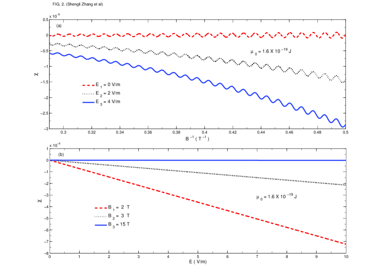
Figure 2: $\left(a\right)$ Magnetic susceptibility $\chi$ depends on reciprocal field $1/B$ for a given chemical potential $\mu_{0}=1.6\times 10^{-19}~{}\mbox{J}$ and $T=0~{}\mbox{K}$. Three oscillation curves of magnetic susceptibility correspond to $E_{1}=0~{}\mbox{V/m}$, $E_{2}=2~{}\mbox{V/m}$ and $E_{3}=4~{}\mbox{V/m}$, respectively. $\left(b\right)$ $\chi$ as a function of electric field $E$ for $\mu_{0}=1.6\times 10^{-19}~{}\mbox{J}$ and $T=0~{}\mbox{K}$. Three curves correspond to $B_{1}=$ 2 T, $B_{2}=$ 3 T and $B_{3}=$ 15 T, respectively.

Figure 2(a) shows that the magnetic susceptibility $\chi$ oscillates periodically as a function of $1/B$ and the period follows Eq. (9). Three oscillation curves correspond to $E_{1}=0~{}\mbox{V/m}$, $E_{2}=2~{}\mbox{V/m}$ and $E_{3}=4~{}\mbox{V/m}$, respectively. For the case $(E_{1})$, the reader may observe that the magnetic susceptibility $\chi$ swings between negative and positive values, thus the curve shows a totally orbital diamagnetic to paramagnetic transition. As for the finite electric fields, one can see that the magnetic susceptibility decreases in company with the periodic oscillation while $1/B$ rising and the $OA$ augments as $1/B$ increases. Furthermore, from Eq. (28) it can be seen that the $OA$ increases to infinity at $\beta_{c}=1$, leading to the vanishing of $dHvA$ effect on magnetic susceptibility. In general, the magnetic susceptibility $\chi$ is a constant in usual electron gas, but in graphene it exhibits the dependence on the external field.

Figure 2(b) depicts the magnetic susceptibility $\chi$ with respect to the electric field E. Three curves correspond to $B_{1}=2~{}\mbox{T}$, $B_{2}=3~{}\mbox{T}$ and $B_{3}=15~{}\mbox{T}$, respectively. As is shown by the three curves, the magnetic susceptibility varies approximately linearly with increasing $E$. For $B=2$ T, or 3 T, the magnetic susceptibility decreases as $E$ increases and yields $\chi<0$, indicating the existence of Landau diamagnetism in graphene, the origin of which can be traced to the quantized Landau level. In the case of $B=15~{}\mbox{T}$ or larger, the magnetic susceptibility $\chi\simeq 0$ despite the increase of $E$, suggesting the disappearance of the diamagnetism in graphene. That is, there is no increase in the magnetic susceptibility with increasing $E$. Moreover, the dashed line $(B_{1}=2~{}\mbox{T}$) decreases to negative infinity at the exotic point $E=2\times 10^{6}$ V/m (i.e. $\beta_{c}=1$) as illustrated by Eqs. (26) and (28).

3.2 Finite temperature

We now consider the temperature effect on the oscillations of magnetization and magnetic susceptibility. As documented in [12], the thermodynamic potential of electrons in graphene, can be expressed as

$$\Omega\left(T,\mu\right)=\int_{-\infty}^{\infty}d\omega P_{T}\left(\omega-\mu\right)E\left(\omega\right),$$ (30)

with energy variable $\omega$ and $\mu$. And $P_{T}\left(z\right)$ is the distribution function as

$$P_{T}\left(z\right)=-\frac{\partial n_{F}\left(z\right)}{\partial z}=\frac{1}{4k_{B}T\cosh^{2}\frac{z}{2k_{B}T}}.$$ (31)

Using Eq. $\left(30\right)$, the thermodynamic potential $\Omega$ can be divided as follows:

$$\Omega\left(T,\mu\right)=\Omega_{reg}+\Omega_{add}+\Omega_{osc}.$$ (32)

At the low temperatures, neglecting $0(k_{B}T),$ we can obtain

$$\Omega_{reg}=-\frac{\zeta\left(3/2\right)\upsilon_{F}}{\pi^{2}\sqrt{2\hbar}}\left(eB\right)^{3/2}\left(1-\beta^{2}\right)^{3/4}+\frac{2\mu_{0}^{3}}{3\pi\left(\hbar\upsilon_{F}\right)^{2}}\left(1-\beta^{2}\right)^{3/4},$$ (33)

$$\Omega_{add}=\frac{\pi}{L_{y}}\hbar\upsilon_{F}\beta A_{\Omega_{T}}R_{T}\left(k,\mu\right),$$ (34)

where

$$A_{\Omega_{T}} = \frac{\mu_{0}^{4}}{\pi^{2}\left(\hbar\upsilon_{F}\right)^{4}}-\frac{2eB\mu_{0}^{2}}{\hbar\left(\pi\hbar\upsilon_{F}\right)^{2}}(2\left[\frac{\mu_{0}^{2}}{2e\hbar\upsilon_{F}^{2}B}\right]+1)+\left[\frac{\mu_{0}^{2}}{2e\hbar\upsilon_{F}^{2}B}\right]$$ (35)

$$\times\left(\left[\frac{\mu_{0}^{2}}{2e\hbar\upsilon_{F}^{2}B}\right]+1\right)\left(\frac{2eB}{\hbar\pi}\right)^{2}.$$

This expression involves a dependence on the integer part $[\mu_{0}^{2}/2e\hbar\upsilon_{F}^{2}B]$. And here we introduced the temperature reduction factor

$$R_{T}\left(k,\mu\right)=\frac{2\pi^{2}k\mu_{0}k_{B}T/\left(e\hbar\upsilon_{F}^{2}B^{\ast}\right)}{\sinh\frac{2\pi^{2}k\mu_{0}k_{B}T}{e\hbar\upsilon_{F}^{2}B^{\ast}}},$$ (36)

in which $B^{\ast}=B\left(1-\beta^{2}\right)^{3/4}$. Eq. (36) means that the temperature reduction factor $R_{T}$ depends not only on the temperature, but also on the electric and magnetic fields. We return now to the oscillating part of thermodynamic potential. Substituting Eq. (19) into Eq. (30), it is convenient to get the expression of $\Omega_{osc}$ as

$$\Omega_{osc}\left(T,\mu\right) = \frac{\left(eB\right)^{3/2}\upsilon_{F}}{\sqrt{\hbar}\pi^{3/2}}\left(1-\beta^{2}\right)^{3/4}\sum_{k=1}^{\infty}\frac{1}{\left(\pi k\right)^{3/2}}$$ (37)

$$\times Im[e^{-i\pi/4}\int_{0}^{\infty}\frac{dte^{-i\left(\pi kw\right)t}}{\sqrt{t}\left(t+1\right)}\int_{-\infty}^{\infty}\frac{d\epsilon}{4k_{B}T\cosh^{2}\frac{\left(\epsilon-\mu\right)}{2k_{B}T}}$$

$$\exp\left(\frac{-i\pi k\epsilon^{2}\left(t+1\right)}{e\hbar\upsilon_{F}^{2}B\left(1-\beta^{2}\right)^{3/2}}\right)],$$

in which we used that the function $J_{1}(p,r)$ and $J_{2}(p,r)$ which can be represented as -Im and Re parts of the same function

$$\sqrt{\pi}J_{1}\left(p,r\right) = -Im\int_{0}^{\infty}\frac{dte^{-pt-r/t}}{\sqrt{t}\left(t+i\right)},$$

$$\sqrt{\pi}J_{2}\left(p,r\right) = -Re\int_{0}^{\infty}\frac{dte^{-pt-r/t}}{\sqrt{t}\left(t+i\right)},$$ (38)

and rotated the integration contour to the imaginary axis. Finally we get

$$\Omega_{osc}\left(T,\mu\right)=\frac{\left(eB\upsilon_{F}\right)^{2}}{\pi\mu_{0}}\left(1-\beta^{2}\right)^{3/4}\sum_{k=1}^{\infty}\frac{\cos\left(\pi kw\right)}{\left(\pi k\right)^{2}}R_{T}\left(k,\mu\right),$$ (39)

with $w=\mu_{0}^{2}/\left(e\hbar\upsilon_{F}^{2}B\right)$. Clearly, since $R_{T}\left(k,\mu\right)\rightarrow 1$ for $T\rightarrow 0,$ Eq. (39) reduces to the oscillating energy for zero temperature. When the temperature $T\neq 0,$ the magnetization can be obtained as follows:

$$M_{reg}^{T}=\frac{3e\sqrt{eB\hbar}\zeta\left(3/2\right)\upsilon_{F}}{2\sqrt{2}\pi^{2}\hbar\left(1-\beta^{2}\right)^{1/4}}-\frac{\mu_{0}^{3}\beta^{2}}{\pi\left(\hbar\upsilon_{F}\right)^{2}B\left(1-\beta^{2}\right)^{1/4}},$$ (40)

$$M_{add}^{T}=\frac{\pi\hbar\upsilon_{F}\beta R_{T}}{BL_{y}}A_{M_{0}}-\frac{\pi\hbar\upsilon_{F}\beta\left(2+\beta^{2}\right)}{2BL_{y}\left(1-\beta^{2}\right)}A_{\Omega_{T}}\left(R_{T}^{\ast}-R_{T}\right),$$ (41)

and

$$M_{osc}^{T} = -\frac{e\mu_{0}}{\pi\hbar}\left(1-\beta^{2}\right)^{3/4}\sum_{k=1}^{\infty}\frac{\sin\left(\pi kw\right)}{\pi k}R_{T}-\frac{\left(e\upsilon_{F}\right)^{2}B}{2\pi\mu_{0}\left(1-\beta^{2}\right)^{1/4}}$$ (42)

$$\times[\left(4-\beta^{2}\right)R_{T}+\left(2+\beta^{2}\right)\left(R_{T}^{\ast}-R_{T}\right)]\sum_{k=1}^{\infty}\frac{\cos\left(\pi kw\right)}{\left(\pi k\right)^{2}},$$

where $R_{T}^{\ast}\left(k,\mu\right)=R_{T}^{2}\left(k,\mu\right)\cosh\left(2\pi^{2}k\mu_{0}k_{B}T/e\hbar\upsilon_{F}^{2}B^{\ast}\right)$. Apparently, since $R_{T}\left(k,\mu\right)\rightarrow 1$ and $R_{T}^{\ast}\left(k,\mu\right)\rightarrow 1$ for $T\rightarrow 0,$ Eq. (42) reduces to the magnetization in Eq. (3.1) for zero temperature.

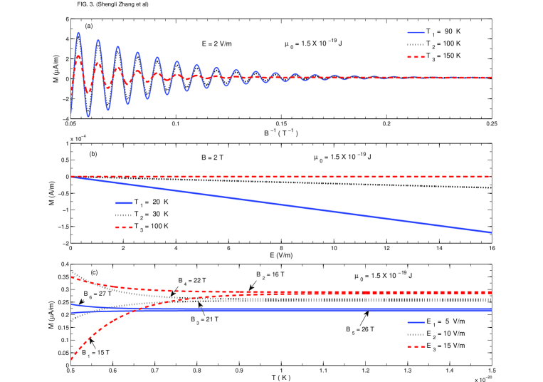
Figure 3: $\left(a\right)$ Magnetization $M$ is plotted as a function of reciprocal magnetic field $1/B$ for a given chemical potential $\mu_{0}=1.5\times 10^{-19}~{}\mbox{J}$ and $E=2~{}\mbox{V/m}$. Three curves correspond to temperature $T_{1}=90~{}\mbox{K}$, $T_{2}=100~{}\mbox{K}$ and $T_{3}=150~{}\mbox{K}$, respectively. $\left(b\right)$  $M$ plotted to electric field $E$ with $B=2$ T and $\mu_{0}=1.5\times 10^{-19}~{}\mbox{J}$. Three curves correspond to $T_{1}=20~{}\mbox{K}$, $T_{2}=30~{}\mbox{K}$ and $T_{3}=100~{}\mbox{K}$, respectively. $\left(c\right)$ $M$ is plotted as a function of temperature $T$ for $\mu_{0}=1.5\times 10^{-19}~{}\mbox{J}$.

As is illustrated in Figure 3(a), finite $T$ causes a reduction of the magnetization amplitude as opposed to the case of $T=0~{}\mbox{K}$. Meanwhile, it shows the magnetization $M$ versus reciprocal field $1/B$ for three different temperatures with a given $E$. It can be seen that as the value of $1/B$ increases, the $OA$ of magnetization decreases and eventually collapses when $\beta\rightarrow 1$. Nevertheless, regarding the zero temperature, there is no such a collapse for the $OA$ of magnetization as shown in Fig. $1(a)$. Accordingly, we attribute them to the finite temperature effect.

Figure 3(b) depicts the magnetization $M$ as a function of $E$ for three different temperatures with a given $B$. Three curves correspond to $T_{1}=20~{}\mbox{K}$, $T_{2}=30~{}\mbox{K}$ and $T_{3}=100~{}\mbox{K}$, respectively. It has been shown that the magnetization decreases approximately linearly with increasing $E$ except in the case of $T_{3}=100~{}\mbox{K}$. Finally, the magnetization decreases to the negative infinity at $\beta_{c}=1$ following Eqs. (40), (41) and (42). At the temperature $T_{3}$ or even a higher one, the magnetization $M\simeq 0$ rather than decrease with increasing $E$. Fig. $3(c)$ gives the magnetization $M$ as function of the temperature $T$. Increasing $T$, the magnetization $M$ increases for $B_{1}$, $B_{3}$, $B_{5}$ and decreases for $B_{2}$, $B_{4}$, $B_{6}$, but they all end up approaching different constants.

We get the $dHvA$ magnetic susceptibility from the magnetization:

$$\chi_{reg}^{T}=\frac{3e\mu_{p0}\sqrt{e\hbar}\varsigma\left(3/2\right)\upsilon_{F}}{4\sqrt{2B}\pi^{2}\hbar\left(1-\beta^{2}\right)^{5/4}}\left(1-2\beta^{2}\right)+\frac{\mu_{0}^{3}\beta^{2}\mu_{p0}\left(6-5\beta^{2}\right)}{2\pi\left(\hbar\upsilon_{F}B\right)^{2}\left(1-\beta^{2}\right)^{5/4}},$$ (43)

$$\chi_{add}^{T} = -\frac{2\mu_{p0}\beta\mu_{0}^{4}R_{T}}{L_{y}B^{2}\left(\hbar\upsilon_{F}\right)^{3}}+\frac{\pi\hbar\upsilon_{F}\mu_{p0}\beta\left(2+\beta^{2}\right)}{B^{2}L_{y}\left(1-\beta^{2}\right)}A_{M_{0}}\left(R_{T}^{\ast}-R_{T}\right)$$ (44)

$$-A_{\chi 0_{T}}A_{\Omega_{T}}\frac{\pi\hbar\upsilon_{F}\mu_{p0}\beta}{L_{y}},$$

and

$$\chi_{osc}^{T}=A_{\chi 1_{T}}\sum_{k=1}^{\infty}\cos\left(\pi kw\right)+A_{\chi 2_{T}}\sum_{k=1}^{\infty}\sin\left(\pi kw\right),$$ (45)

in Eq. (44), $A_{M_{0}}$ and $A_{\Omega_{T}}$ are defined by Eqs. (24) and (35), respectively. We also define,

$$A_{\chi 0_{T}} = \frac{\left(2\beta^{4}-10\beta^{2}-4\right)}{\left[2B\left(1-\beta^{2}\right)\right]^{2}}[R_{T}^{\ast}-R_{T}]+\left(\frac{2+\beta^{2}}{2B\left(1-\beta^{2}\right)}\right)^{2}[2R_{T}$$

$$\times(R_{T}^{\ast}-R_{T})\cosh\frac{2\pi^{2}kT\mu_{0}}{e\hbar\upsilon_{F}^{2}B^{\ast}}-R_{T}^{3}\sinh^{2}\frac{2\pi^{2}kT\mu_{0}}{e\hbar\upsilon_{F}^{2}B^{\ast}}-\left(R_{T}^{\ast}-R_{T}\right)],$$

$$A_{\chi 1_{T}} = \frac{\mu_{0}^{3}\mu_{p0}\left(1-\beta^{2}\right)^{3/4}}{\pi\left(\hbar\upsilon_{F}B\right)^{2}}R_{T}-\frac{\left(e\upsilon_{F}\right)^{2}\mu_{p0}\left(4-\beta^{2}\right)\left(2+\beta^{2}\right)}{2\pi\mu_{0}\left(\pi k\right)^{2}\left(1-\beta^{2}\right)^{5/4}}\left(R_{T}^{\ast}-R_{T}\right)$$

$$-R_{T}\frac{\left(e\upsilon_{F}\right)^{2}\mu_{p0}(8-10\beta^{2}-\beta^{4})}{4\pi\mu_{0}\left(\pi k\right)^{2}\left(1-\beta^{2}\right)^{5/4}}-\frac{A_{\chi 0_{T}}\mu_{p0}\left(e\upsilon_{F}B\right)^{2}}{\pi\mu_{0}\left(\pi k\right)^{2}}\left(1-\beta^{2}\right)^{3/4},$$

$$A_{\chi 2_{T}}=-\frac{e\mu_{0}\mu_{p0}\left(2+\beta^{2}\right)}{\pi^{2}\hbar kB\left(1-\beta^{2}\right)^{1/4}}R_{T}^{\ast}.$$ (48)

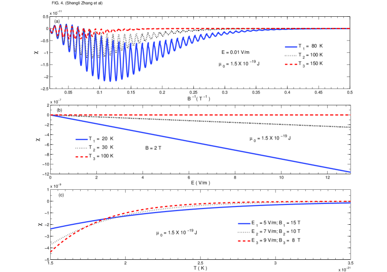
Figure 4: $\left(a\right)$ Magnetic susceptibility $\chi$ to reciprocal field $1/B$ for a given chemical potential $\mu_{0}=1.5\times 10^{-19}~{}\mbox{J}$ and $E=0.01~{}\mbox{V/m}$. Three oscillation curves of magnetic susceptibility correspond to $T_{1}=80~{}\mbox{K}$, $T_{2}=100~{}\mbox{K}$ and $T_{3}=150~{}\mbox{K}$, respectively. $\left(b\right)$ $\chi$ as a function of electric field $E$ with $B=$ 2 T and $\mu_{0}=1.5\times 10^{-19}~{}\mbox{J}$. Three oscillation curves of magnetic susceptibility correspond to $T_{1}=20~{}\mbox{K}$, $T_{2}=30~{}\mbox{K}$ and $T_{3}=100~{}\mbox{K}$, respectively. $\left(c\right)$ $\chi$ as a function of temperature $T$ for $\mu_{0}=1.5\times 10^{-19}~{}\mbox{J}$.

Figure 4(a) shows the magnetic susceptibility $\chi$ oscillates periodically as a function of $1/B$, for three characteristic temperatures, namely, 80, 100, and 150 K. Similar to the magnetization as shown in Fig. $3(a)$, it also exhibits the dependence on temperature. It can be seen clearly that finite $T$ causes a reduction of the oscillation amplitude and as the value of $1/B$ increases, the $OA$ of magnetic susceptibility finally decays to zero.

Figure 4(b) shows the magnetic susceptibility $\chi$ plotted as a function of $E$ with a given $B$. Three curves correspond to $T_{1}=20~{}\mbox{K}$, $T_{2}=30~{}\mbox{K}$ and $T_{3}=100~{}\mbox{K}$, respectively. For a finite temperature such as $T_{1}$ or $T_{2}$, the magnetic susceptibility decreases approximately linearly with increasing $E$ and exhibits the Landau diamagnetism in graphene supported by $\chi<0$. In contrast, at the temperature $T_{3}$, the magnetic susceptibility $\chi\simeq 0$, standing for the disappearance of the diamagnetism in graphene. In addition, there is no increase in the magnetic susceptibility with increasing $E$. It warrants great attention that from Eqs. (43), (44) and (45), it could be inferred that the magnetic susceptibility eventually decreases to the negative infinity at $\beta_{c}=$ 1. Fig. $4(c)$ directly gives the magnetic susceptibility $\chi$ with respect to the temperature $T$. More specifically, it shows that the magnetic susceptibility $\chi$ increases with increasing $T$ and finally approaches zero under different electric field $Es$ and the magnetic field $Bs$.

4 Conclusions

In summary, this paper reports on a theoretical study on the modulation of de Haas-van Alphen effect in graphene by electric field. Three major findings emerge from the study. First of all, we find that both magnetization and magnetic susceptibility are modulated by the electric field. At the zero or finite temperature, both magnetization and magnetic susceptibility are predicted to oscillate periodically as a function of reciprocal field $1/B$. The $dHvA$ oscillation period $\Delta(1/B)$ is derived analytically. It is also discovered that as the parameter $\beta$ increases, the values of magnetization and magnetic susceptibility finally increase to positive infinity or decrease to negative infinity at the exotic point $\beta_{c}=1$. Besides, the analytical results indicate that the $dHvA$ oscillation amplitude increases abruptly to infinity for zero temperature at $\beta_{c}=1$, but eventually collapses at a finite temperature directly leading to the vanishing of the de Haas-van Alphen effect. The ”vanishing” is accounted for the anomalous effect of the electric field on Landau level, which arises from the instability of a relativistic quantum field vacuum. In addition, it is established that the magnetic susceptibility depends on the electric and magnetic fields, which suggests the graphene should be a non-linear magnetic medium. These phenomena, not available in the standard 2D electron gas, are deemed as the consequence of the relativistic type spectrum of low energy electrons and holes in graphene.

5 Acknowledgments

We thank Dr D. Q. Liu, Q. Wang, X. H. Zhang, B. H. Gong, L. Xu, and H. W. Chen for helpful discussions. This work is supported by the Cultivation Fund of the Key Scientific and Technical Innovation Project Ministry of Education of China (NO 708082).

References

• [1] Novoselov K S, Geim A K, Morozov S V, Jiang D, Zhang Y, Dubonos S V, Grigorieva I V and Firsov A A 2004 Science 306 666
• [2] Novoselov K S, Jiang D, Schedin F, Booth T J, Khotkevich V V, Morozov S V and Geim A K 2005 Proc. Natl. Acad. Sci. U.S.A. 102 10451
• [3] Zhang Y, Small J P, Amori M E S and Kim P 2005 Phys. Rev. Lett. 94 176803
• [4] Li G and Andrei E Y 2007 Nature physics. 3 623
• [5] Kane C L and Mele E J 2005 Phys. Rev. Lett. 95 226801
• [6] Haldane F D M 1988 Phys. Rev. Lett. 61 2015
• [7] Sinitsyn N A, Hill J E, Min H, Sinova J and MacDonald A H 2006 Phys. Rev. Lett. 97 106804
• [8] Yao W, Yang S A and Niu Q 2009 Phys. Rev. Lett. 102 096801
• [9] Wilson M 2006 Phys. Today 59(1) 21
• [10] Novoselov K S, Geim A K, Morozov S V, Jiang D, Katsnelson M I, Grigorieva I V, Dubonos S V and Firsov A A 2005 Nature 438 197
• [11] Zhang Y B, Tan Y W, Stormer H L and Kim P 2005 Nature 438 201; Zhang Y, Jiang Z, Small J P, Purewal M S, Tan Y W, Fazlollahi M, Chudow J D, Jaszczak J A, Stormer H L and Kim P 2006 Phys. Rev. Lett. 96 136806
• [12] Sharapov S G, Gusynin V P and Beck H 2004 Phys. Rev. B 69 075104
• [13] Peierls R 1933 Z. Phys. 81 186
• [14] Landau L D and Lifshitz E M 1971 Relativistic Quantum Theory (Pergamon, New York) p. 100.
• [15] Lukose V, Shankar R and Baskaran G 2007 Phys. Rev. Lett. 98 116802
• [16] Callaway J 1976 Quantum Theory of the Solid State New York: Academic Press
• [17] Shoenberg D 1984 Magnetic Oscillations in Metals Cambridge: Cambridge University Press
• [18] Gradshtein I S and Ryzhik I M 1980 Table of Integrals, Series and Products (Academic Press, Orlando)
• [19] Wilde M A, Schwarz M P, Heyn C, Heitmann D, Grundler D, Reuter D and Wieck A D 2006 Phys. Rev. B 73 125325
• [20] Simserides C 2009 J. Phys.: Condens. Matter 21 015304
• [21] Hu J and MacDonald A H 1992 Phys. Rev. B 46 12554