Non-Markovian master equation for a damped oscillator with time-varying parameters

Abstract

We derive an exact non-Markovian master equation that generalizes the previous work [Hu, Paz and Zhang, Phys. Rev. D 45, 2843 (1992)] to damped harmonic oscillators with time-varying parameters. This is achieved by exploiting the linearity of the system and operator solution in Heisenberg picture. Our equation governs the non-Markovian quantum dynamics when the system is modulated by external devices. As an application, we apply our equation to parity kick decoupling problems. The time-dependent dissipative coefficients in the master equation are shown to be modified drastically when the system is driven by $\pi$ pulses. For coherence protection to be effective, our numerical results indicate that kicking period should be shorter than memory time of the bath. The effects of using soft pulses in an ohmic bath are also discussed.

I Introduction

An oscillator linearly coupled with a harmonic oscillator bath has been an important model for studying quantum dissipation and decoherence. While the solution for the damped harmonic oscillator is well-known under Born- and/or Markov-approximation Breuer ; Weiss ; Gardiner ; Carmichael , general treatments waiving those approximations did not appear until studies of Wigner functions by Haake and Reibold Haake who addressed the issues in low temperature and strong damping regimes. Exact non-Markovian master equation for the model was later derived by Hu, Paz and Zhang (HPZ) HPZ who employed the path-integral approach for initially factorizable states. The use of Wigner function Yu ; Connell and characteristic functions Pereverzev presented alternative means to derive the master equation. The study was generalized by Karrlein and Grabert Karrlein with path-integral approach to cover non-factorizable initial states, who also pointed out that the exact Liouville operator for a damped harmonic oscillator is not independent of initial system states in general. Recently, non-Markovian master equations have been generalized to two-oscillator problems in order to study quantum disentanglement processes Hu2008 ; Oh2 ; Paris1 ; Paris2 ; Roncaglia .

In parallel with these advances, there is a growing interest in coherence protection due to the need of preserving quantum information stored in a system that is inevitably coupled with its environment Viola . In particular, dynamical decoupling techniques for two-level systems based on various pulses sequences have been developed and optimized Agarwal ; Uhrig1 ; Uhrig2 ; Uhrig3 ; Kurizki . For damped harmonic oscillator systems, parity kicks by a stream of $\pi$ pulses is a conceptually simple strategy in realizing dynamical decoupling Viola ; Tombesi1 . Such a strategy has been studied primarily in the $\delta$-pulse regime Tombesi1 ; Tombesi2 ; ShiokawaHu , but little was explored in the soft-pulse regime. In order to address the problem one needs to establish equations describing the dissipation dynamics for systems driven by time-varying external fields.

The main purpose of this paper is to present an exact non-Markovian master equation for an oscillator with time-varying parameters in general. Such time-varying parameters correspond to the modulation of oscillator frequency and parametric interactions strengths caused by external devices. As a demonstrative example, we apply our master equation to study the dynamics in ‘parity kick’ problems. Numerical results of dissipative coefficients in the master equation are found to be drastically modified by the $\pi$ pulses. By solving the master equation, we also address the effectiveness of coherence protection, quantified by fidelity ${\cal F}(t)$ of system state, at various kicking frequencies with soft pulses.

II The Master Equation

We consider an oscillator coupled linearly with an oscillator bath the total Hamiltonian $H=H_{S}(t)+H_{B}+H_{I}$, where

$$H_{S}(t) = \frac{\lambda(t)}{2}a^{2}+\frac{{\lambda^{\ast}(t)}}{2}{a^{\dagger 2}}+\left[\omega_{0}+\Omega(t)\right]a^{\dagger}a{}$$ (1)

$$H_{B} = \sum_{k}\omega_{k}b_{k}^{\dagger}b_{k}$$ (2)

$$H_{I} = \sum_{k}g_{k}(a+a^{\dagger})(b_{k}+b_{k}^{\dagger}).$$ (3)

Here the system oscillator has a time-dependent natural frequency $\omega_{0}+\Omega(t)$ and a parametric coupling strength $\lambda(t)$. With these time-dependent parameters, we treat in generality the time-dependent damped harmonic oscillator problem, which distinguishes our work from previous studies. Physically, the frequency shift $\Omega(t)$ can be induced by off-resonance driving fields, and $\lambda(t)$ describes time-dependent parametric effects, for example in down conversion processes in nonlinear optics. In our model the bath consists of a large number of oscillators, with $\omega_{k}$ and real coupling strength $g_{k}$ being the frequency and coupling strength of the $k$-th mode oscillator. We also define the annihilation operators of the system oscillator and the bath oscillators by $a\equiv\sqrt{\frac{m\omega_{0}}{2}}\left(X+\frac{iP}{m\omega_{0}}\right)$ and $b_{k}\equiv\sqrt{\frac{m_{k}\omega_{k}}{2}}\left(q_{k}+\frac{ip_{k}}{m_{k}\omega_{k}}\right)$. Here $X$ and $P$ are position and momentum operators of system oscillator with mass $m$ and frequency $\omega_{0}$, while $q_{k}$ and $p_{k}$ are position and momentum operators of $k$-th mode of bath oscillator with mass $m_{k}$.

The bath structure is characterized by spectral density $J(\omega)\equiv\sum_{k}g_{k}^{2}\delta(\omega-\omega_{k})$. In the limit $\omega_{k}$ becomes continuum, we adopt the commonly used spectral density of the form

$$J(\omega)=\eta\omega\left(\frac{\omega}{\omega_{c}}\right)^{n-1}e^{-\frac{\omega}{\omega_{c}}}$$ (4)

where $\eta$ is a dimensionless real number governing the strength of system-bath coupling, and $\omega_{c}$ is the cut-off frequency. Necessity and justification to introduce cut-off frequency have been discussed in Weiss . The exponent $n$ is a real number that determines the $\omega$-dependence of $J(\omega)$ in the low frequency region, and for physical baths $n\geq 0$. In literatures, $0<n<1$, $n=1$ and $n>1$ are termed as ‘subohmic’, ‘ohmic’ and ‘superohmic’ baths respectively. We will focus on ohmic bath as an example given in Sec. III.

To derive the master equation, we first consider the initial total density matrix of the factorizable form:

$$\rho_{tot}(0) = |\alpha_{0}\rangle\langle\alpha_{0}|$$ (5)

$$\otimes\prod_{k}\left[(e^{-\hbar\omega_{k}b_{k}^{\dagger}b_{k}/k_{B}T})(1-e^{-\hbar\omega_{k}/k_{B}T})\right]$$

where $|\alpha_{0}\rangle$ is a coherent state for system and the bath is initially in thermal equilibrium at temperature $T$. At later time $t>0$, the total density matrix in position-space representation reads

$$\rho_{tot}(X^{\prime\prime},{\bf q^{\prime\prime}},X^{\prime},{\bf q^{\prime}},t)$$ (6)

$$= \int\!dXd{\bf q}\int\!dX^{\prime\prime\prime}d{\bf q^{\prime\prime\prime}}\,U(X^{\prime\prime},{\bf q^{\prime\prime}},t;X,{\bf q},0)$$

$$\times\rho_{tot}(X,{\bf q},X^{\prime\prime\prime},{\bf q^{\prime\prime\prime}},0)U^{\ast}(X^{\prime},{\bf q^{\prime}},t;X^{\prime\prime\prime},{\bf q^{\prime\prime\prime}},0)$$

where $\rho_{tot}(X^{\prime\prime},{\bf q^{\prime\prime}},X^{\prime},{\bf q^{\prime}},0)\equiv\langle X^{\prime\prime},{\bf q^{\prime\prime}}|\rho_{tot}(0)|X^{\prime},{\bf q^{\prime}}\rangle$, where ${\bf q}\equiv(\{q_{k}\})$ and $U(X^{\prime\prime},{\bf q^{\prime\prime}},t;X^{\prime},{\bf q^{\prime}},0)\equiv\langle X^{\prime\prime},{\bf q^{\prime\prime}}|{\cal T}\exp\left[-i\int_{0}^{t}\!ds\,H(s)\right]|X^{\prime},{\bf q^{\prime}}\rangle$, with ${\cal T}$ being the time-ordering operator. The factorized initial density matrix (5) guarantees that the Liouville operator is independent of initial system state, which was also observed in HPZ ; Connell ; Yu . The Guassian initial state (5) and the Gaussian kernel in Eq. (6) resulted from the linearity of total Hamiltonian allow exact integration, which makes the reduced density matrix $\rho_{S}={\rm Tr}_{B}(\rho_{tot})$ also a Gaussian. In other words, the master equation governing the evolution of $\rho_{S}$ must preserve the Gaussian properties. This requires that the master equation involves only some quadratic combinations of $a$ and $a^{\dagger}$ as in the HPZ master equations. Together with the requirements of conservation of probability [${\rm Tr}(\dot{\rho}_{S})=0$], hermiticity ($\rho_{S}=\rho_{S}^{\dagger}$) and state-independent coefficients ($\gamma_{1}$, $\gamma_{2}$, $\gamma_{3}$, $\Delta\omega$ and $\Delta\lambda$ in below), we have the following form of time-convolutionless master equation:

$$\dot{\rho}_{S} = -i\left[{H_{S}(t)+\Delta H_{S}(t),\rho_{S}}\right]$$ (7)

$$-\gamma_{1}(t)\left({a^{\dagger}a\rho_{S}+\rho_{S}a^{\dagger}a-2a\rho_{S}a^{\dagger}}\right)$$

$$-\gamma_{2}(t)\left({aa^{\dagger}\rho_{S}+\rho_{S}aa^{\dagger}-2a^{\dagger}\rho_{S}a}\right)$$

$$-\gamma_{3}(t)\left({aa\rho_{S}+\rho_{S}aa-2a\rho_{S}a}\right)$$

$$-\gamma_{3}^{\ast}(t)\left({a^{\dagger}a^{\dagger}\rho_{S}+\rho_{S}a^{\dagger}a^{\dagger}-2a^{\dagger}\rho_{S}a^{\dagger}}\right)$$

where

$$\Delta H_{S}(t)=\frac{{\Delta\lambda(t)}}{2}a^{2}+\frac{{\Delta\lambda^{*}(t)}}{2}a^{\dagger 2}+\Delta\omega(t)a^{\dagger}a$$ (8)

are modifications to the system Hamiltonian due to system-bath interaction. In particular, $\Delta\omega(t)$ is the frequency shift term, $\Delta\lambda(t)$ modifies the parametric interaction, $\gamma_{1}(t)$ and $\gamma_{2}(t)$ are functions governing dissipation and amplification, and the terms with $\gamma_{3}(t)$ describe phase-dependent decoherence typically appear in squeezed baths Gardiner .

Our next task is to determine the time-dependent coefficients. To this end, with the formal solution of $b_{k}(t)$, let us write down the Heisenberg’s equation for $a(t)$,

$$\dot{a}(t) = -i\lambda^{\ast}(t)a^{\dagger}(t)\!-\!i\left[\omega_{0}+\Omega(t)\right]a(t)$$ (9)

$$-i\sum_{k}g_{k}\left[b_{k}(0)e^{-i\omega_{k}t}+b_{k}^{\dagger}(0)e^{i\omega_{k}t}\right]$$

$$-\!\int_{0}^{t}\!ds\,K(t-s)\left[a(s)+a^{\dagger}(s)\right]$$

where $K(\tau)$ is the memory kernel and $K(\tau)\equiv-2i\sum_{k}g_{k}^{2}\sin\omega_{k}\tau=-2i\int_{0}^{\infty}\!d\omega\,J(\omega)\sin\omega\tau$.

The linearity of Eq. (9) leads to a general operator solution for $a(t\geq 0)$ that can be expressed in terms of initial conditions,

$${a}(t)=G(t)\,{a}(0)+L^{\ast}\!(t)\,a^{\dagger}(0)+{F}(t)$$ (10)

where $F(t)=\sum_{k}\left(\mu_{k}(t)b_{k}(0)+\nu_{k}^{\ast}(t)b_{k}^{\dagger}(0)\right)$. The functions $G(t)$, $L(t)$, $\mu_{k}(t)$ and $\nu_{k}(t)$ can be determined by substituting Eq. (10) into Eq. (9) and comparing coefficients of initial system operators. This gives,

$$\dot{G} = -i\lambda^{\ast}(t)L-i\left[\omega_{0}+\Omega(t)\right]G$$ (11)

$$-\!\int_{0}^{t}\!ds\,K(t-s)\,\left[G(s)+L(s)\right],$$

$$\dot{L} = i\lambda(t)G+i\left[\omega_{0}+\Omega(t)\right]L$$ (12)

$$+\!\int_{0}^{t}\!ds\,K(t-s)\,\left[G(s)+L(s)\right],$$

$$\dot{F} = -i\lambda^{\ast}(t)F^{\dagger}-i\left[\omega_{0}+\Omega(t)\right]F$$ (13)

$$-\!\int_{0}^{t}\!ds\,K(t-s)\left[F(s)+F^{\dagger}(s)\right]$$

$$-i\sum_{k}g_{k}\left[b_{k}(0)e^{-i\omega_{k}t}+b^{\dagger}_{k}(0)e^{i\omega_{k}t}\right]$$

with initial conditions $G(0)=1$, $L(0)=0$, $\mu_{k}(0)=0$ and $\nu_{k}(0)=0$ (see Appendix A for further reduction on $F(t)$). Hence for a given spectral density $J(\omega)$ and system Hamiltonian, $G(t)$ and $L(t)$ can be solved and the operator solution $a(t)$ can be found.

Now we make use of the fact that the time derivative for $\langle a(t)\rangle$, $\langle a(t)a(t)\rangle$ and $\langle a^{\dagger}(t)a(t)\rangle$ obtained by the master equation (7) must agree with that obtained by the corresponding Heisenberg operator solution after taking expectation values. A direct comparison of these equations (see Appendix B for details) allows us to determine $\gamma_{1}$, $\gamma_{2}$, $\gamma_{3}$, $\Delta\omega$ and $\Delta\lambda$. It is easy to show in the comparison that

$$\Delta\lambda=\Delta\omega-i(\gamma_{1}-\gamma_{2})$$ (14)

which is not independent from other time-dependent coefficients, and the remaining coefficients are:

$$2i\Delta\omega = \frac{1}{W(t)}\int_{0}^{t}\!ds\,K(t-s)\,$$ (15)

$$\{\left[G(t)-L(t)\right]\left[L^{\ast}(s)+G^{\ast}(s)\right]$$

$$\hskip 14.22636pt+\left[G^{\ast}(t)-L^{\ast}(t)\right]\left[G(s)+L(s)\right]\}$$

$$\gamma_{1} = -\frac{1}{2}\frac{\dot{W}(t)}{W(t)}+\gamma_{2}$$ (16)

$$2\gamma_{2} = \frac{d}{dt}\langle F^{\dagger}F\rangle-\frac{\dot{W}(t)}{W(t)}\langle F^{\dagger}F\rangle$$ (17)

$$-\frac{\dot{L}G^{\ast}-\dot{G}^{\ast}L}{W(t)}\langle FF\rangle$$

$$-\frac{\dot{L}^{\ast}G-\dot{G}L^{\ast}}{W(t)}\langle F^{\dagger}F^{\dagger}\rangle$$

$$-2\gamma_{3}^{\ast} = \frac{d}{dt}\langle FF\rangle-2\frac{\dot{G}G^{\ast}-\dot{L}^{\ast}L}{W(t)}\langle FF\rangle$$ (18)

$$-\frac{\dot{L}^{\ast}G-\dot{G}L^{\ast}}{W(t)}\langle F^{\dagger}F+FF^{\dagger}\rangle$$

where $W(t)\equiv G(t)G^{\ast}(t)-L(t)L^{\ast}(t)$ and the bath-bath correlation functions are

$$\langle F(t)F(t)\rangle = -\int_{0}^{t}\!ds^{\prime}\int_{0}^{t}\!ds^{\prime\prime}\,\kappa_{T}(s^{\prime\prime}-s^{\prime})$$ (19)

$$\left[G(s^{\prime})-L^{\ast}(s^{\prime})\right]\left[G(s^{\prime\prime})-L^{\ast}(s^{\prime\prime})\right]$$

$$\langle F^{\dagger}(t)F(t)\rangle = \int_{0}^{t}\!ds^{\prime}\int_{0}^{t}\!ds^{\prime\prime}\,\kappa_{T}(s^{\prime\prime}-s^{\prime})$$ (20)

$$\left[G^{\ast}(s^{\prime})-L(s^{\prime})\right]\left[G(s^{\prime\prime})-L^{\ast}(s^{\prime\prime})\right]$$

$$\langle F(t)F^{\dagger}(t)\rangle = \int_{0}^{t}\!ds^{\prime}\int_{0}^{t}\!ds^{\prime\prime}\,\kappa_{T}(s^{\prime\prime}-s^{\prime})$$ (21)

$$\left[G(s^{\prime})-L^{\ast}(s^{\prime})\right]\left[G^{\ast}(s^{\prime\prime})-L(s^{\prime\prime})\right]$$

The temperature-dependent memory kernel $\kappa_{T}(\tau)$ takes the form

$$\kappa_{T}(\tau)\equiv\sum_{k}g_{k}^{2}\left[2\cos\left(\omega_{k}\tau\right)\left(e^{\frac{\hbar\omega_{k}}{k_{B}T}}-1\right)^{-1}+e^{-i\omega_{k}\tau}\right]$$ (22)

for a thermal bath at temperature $T$. In particular, at zero temperature,

$$\kappa_{0}(\tau)\equiv\sum_{k}g_{k}^{2}e^{-i\omega_{k}\tau}.$$ (23)

In the special case $\Omega(t)=\lambda(t)=0$, we have ${\rm Re}(\gamma_{3})=(\gamma_{1}+\gamma_{2})/2$ and our equation can be reduced to HPZ master equation.

Since the master equation (7) works for any initial system coherent state $|\alpha_{0}\rangle$, we can generalize the results to arbitrary initial system states by using the Glauber-Sudarshan P-representation. This is because for an arbitrary system state, we can formally express its density matrix in the diagonal form,

$$\rho_{S}(0)=\int\!d^{2}\alpha\,P(\alpha)|\alpha\rangle\langle\alpha|.$$ (24)

By the linearity of (7) and the fact that all the coefficients are independent of initial $\alpha_{0}$, we can conclude that the master equation (7) is also valid for any initial system states.

III Example: Parity kick control

The master equation (7) with the coefficients given in Eq. (15-18) is the main result of this paper. Such an equation provides a useful tool to determine the behavior of a damped harmonic oscillator subjected to external modulation of system parameters. To provide an explicit example, we employ our master equation to study the dynamics in ‘parity kick’ decoherence control problems. Previous studies of this subject were mostly confined to ideal $\delta$-pulses or square pulses that have finite discontinuous jumps Tombesi1 ; Tombesi2 ; ShiokawaHu . In this section we examine parity kick with soft pulses and its efficiency. Specifically, we consider the system Hamiltonian $H_{S}(t)$ in Eq. (1) with $\lambda(t)=0$ and

$$\Omega(t)=\sum_{n}\frac{2\pi}{\epsilon}\{-\phi(\epsilon,n\tau+\frac{\tau}{4},t)+\phi(\epsilon,n\tau+\frac{3\tau}{4},t)\}$$ (25)

where

$$\phi(\epsilon,s,t) \equiv \theta\left[t-\left(s-\frac{\epsilon}{2}\right)\right]\theta\left[\left(s+\frac{\epsilon}{2}\right)-t\right]$$ (26)

$$\times\sin^{2}\left[\frac{\pi}{\epsilon}\left(t-s+\frac{\epsilon}{2}\right)\right]$$

and $\theta(t)$ is the unit-step function. The driving frequency $\Omega(t)$ corresponds to a pair of sine-squared pulses within one pulse period $n\tau\leq t<(n+1)\tau$, each with pulse duration characterized by $\epsilon$, and they peak at $t=n\tau+\frac{\tau}{4}$ and $t=n\tau+\frac{3\tau}{4}$ with strengths $-\pi$ and $\pi$ respectively (see Fig. 1). The idea of using pulses with alternating signs has been discussed in ShiokawaHu . The pair of $\pi$ pulses with zero pulse width ($\epsilon\rightarrow 0$) can effectively reverse the direction of interaction. If the system and bath start uncoupled, then one can prevent the system from coupling with the bath at later times by applying Dirac-delta shaped pulses frequently.

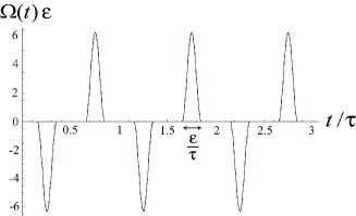
Figure 1: Sketch of the pulses in three periods with $\tau/2$ being the time between successive peaks. Here $\epsilon/\tau=0.2$ is used.

For ideal Dirac-delta shaped pulses $(\epsilon\to 0)$, the pulse width is so short and the strength so strong as that Eqs. (11) and (12) yield $\dot{G}(t)\approx-i\pi\delta(t-t_{0})G(t)$ and $\dot{L}(t)\approx i\pi\delta(t-t_{0})L(t)$ around $t=t_{0}$ where the $\pi$-strength pulse peaks. Integrating, we observe that the sole effect of such an ideal pulse is to flip the sign of $G(t)$ and $L(t)$, while leaving $\dot{G}(t)$ and $\dot{L}(t)$ unchanged, i.e., $G(t_{0}^{-})\rightarrow-G(t_{0}^{+})$, $\dot{G}(t_{0}^{-})\rightarrow\dot{G}(t_{0}^{+})$, $L(t_{0}^{-})\rightarrow-L(t_{0}^{+})$ and $\dot{L}(t_{0}^{-})\rightarrow\dot{L}(t_{0}^{+})$. This leads to the sign-flip of coefficients $\gamma_{1}$, $\gamma_{2}$, $\gamma_{3}$ and $\Delta\omega$ of the above master equation.

However, we point out that while the coefficients of master equation (7) acquire negative sign immediately after the kick, it does not necessarily constitute an effective scheme in coherence protection. Typically memory time characterizes the transient time before the coefficients eventually settle at their long-time limits with the system decaying steadily. Frequent kicking leads to quick and repeating sign-flips that inhibits the free evolution of the coefficients $\gamma_{j}(t)$ and their subsequent settlements, which also produces sawtooth-like graphs for the coefficients. The dissipative coefficients would average to zero over an extended period of time and thus protect the system state and coherence from decaying. Specifically, for an effective scheme the kicking period $\tau$ should be less than the memory time, which is of the order $1/\omega_{c}$, in order to achieve good coherence protection. Vitali and Tombesi Tombesi1 also pointed out that high-frequency bath oscillators with $\omega_{k}\gg\omega_{0}$ would not be able to evolve significantly before interaction Hamiltonian changes sign if a kicking frequency much higher than cut-off frequency is used. Memory time, or equivalently the inverse of cut-off frequency, then plays an important role in fixing the coherence protection scheme. In light of this, the ideal decoupling pulse sequence would consist of pulses with width $\epsilon\rightarrow 0$ and pulse period $\tau\ll 1/\omega_{c}$. More discussions about the use of $\delta$-pulses can be found in Tombesi1 ; Tombesi2 ; ShiokawaHu .

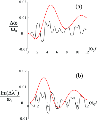
Figure 2: (Colour online) Black solid line: Time-dependence of modification of oscillation frequency (a) and the imaginary part of parametric coupling (b), with $\eta=0.2$, $\omega_{c}/\omega_{0}=0.2$. $\epsilon/\tau=0.5$ and $\omega_{0}\tau=2.0$. Red dashed line correspond to cases without parity kicks for comparison. The bath is ohmic at zero temperature.

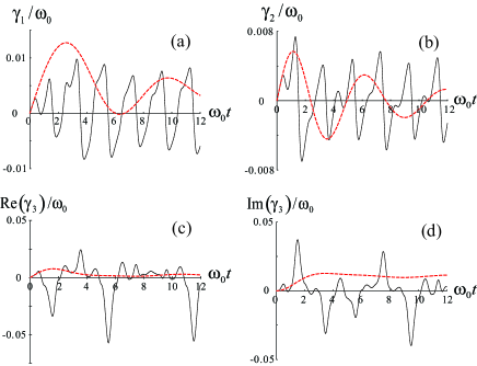
Figure 3: (Colour online) Black solid line: Time-dependence of relaxation coefficients of the master equation for an ohmic bath at zero temperature with $\eta=0.2$, $\omega_{c}/\omega_{0}=0.2$, $\epsilon/\tau=0.5$ and $\omega_{0}\tau=2.0$. Red dashed lines correspond to cases without parity kicks for comparison. The bath is ohmic at zero temperature.

For soft pulses, we can obtain numerically the time-dependent coefficients of master equation according to the prescription in Sec. II. An example is given in Figs. 2 and 3 in which we can compare the coefficients of master equation under the influence of soft-pulse kicks with the free-evolution scenario. In our calculations, we consider an ohmic bath at zero temperature. The parameters $\eta$ and $\omega_{c}$ are chosen such that non-Markovian features, including transient behaviour and non-exponential decay of coherence, can be observed for several natural oscillation cycles. In Fig. 2 we show the modifications of system Hamiltonian $\Delta H_{S}$ in Eq. (8) due to the bath interaction. Without kicking (red dashed lines), $\Delta\omega$ and $\Delta\lambda$ are seen to exhibit oscillatory patterns with frequency close to the natural frequency $\omega_{0}$ of the system. The effect of parity kicks (black solid lines) seem to suppress partially both $\Delta\omega$ and $\Delta\lambda$ with complicated oscillations that follow the kicking frequency $1/\tau$ when ‘parity kick’ is in place. In Fig. 3 the time-dependence of dissipative coefficients $\gamma_{1}$, $\gamma_{2}$ and $\gamma_{3}$ are shown. We note that perfect sign-flip is not present in the figures due to the use of soft pulses. Instead, $\gamma_{1}$ and $\gamma_{2}$ display sawtooth-like periodic oscillations, which average to numbers close to zero in the long run.

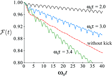
Figure 4: (Color online) Evolution of fidelity ${\cal F}(t)$ subjected to soft pulses with $\omega_{0}\epsilon=1.0$ and various kicking period $\tau$. The parameters are: $\eta=0.2$, $\omega_{c}/\omega_{0}=0.2$ and an ohmic bath at zero temperature.

With the coefficients solved, we proceed to examine the dissipation decay of an initially excited system. As an illustration, we consider the initial state $|\psi_{S}(0)\rangle=|1\rangle$, where $|1\rangle$ is the first excited energy eigenstate of the system. The efficiency of decoherence protection is quantified by the fidelity ${\cal F}(t)\equiv\sqrt{\langle\psi_{S}(0)|\rho_{S}(t)|\psi_{S}(0)\rangle}$ for the pure initial system state. For an ohmic bath and at zero temperature, we observe in Fig. 4 that free evolution (without kicks) no longer gives an exponentially decaying fidelity, and the initial slip is obvious. Our numerical results indicate that parity kicks with soft pulses can suppress the decay if $\tau$ is sufficiently short. However, we notice a transition from coherence protection to decoherence acceleration with increasing pulse period, despite the fact that the pulse periods used in Fig. 4 are all shorter than characteristic memory time of the bath. This is related to the anti-Zeno effect antizeno , and it has been discussed the $\delta$-pulse limit in Ref. ShiokawaHu where the authors suggested that this transition, which occurs when $\tau\sim 1/\omega_{c}$, is not unique to ohmic bath. We have also performed other simulations (not shown) for soft pulses with various widths. For the same parameters in Fig. 4, we find that increasing the width $\epsilon$ would slightly decrease the fidelity.

IV Conclusion

We have derived an exact non-Markovian master equation for a damped harmonic oscillator linearly coupled with an oscillator thermal bath, with a time-dependent natural frequency and parametric interaction strength. The equation enables us to determine the evolution of system density matrix under the influence of various pulses or signals. Expressions of the coefficients of master equation as well as the correlation functions are computable once we solve the functions $G(t)$ and $L(t)$. We emphasize that the method works because of the linearity of the whole system, which leads to the Gaussian propagator, so that we need only to consider a finite number of equations. Our approach has been applied to parity kick problems using soft pulses, and we observe that coefficients of master equations exhibit complicated time-dependence when the system frequency is modulated by $\pi$-pulses. In particular, our numerical results suggest that suppression of decoherence can be achieved by soft pulses, as long as the kicking frequency sufficiently higher than cut-off frequency of the bath.

Appendix A derivation of $G$, $L$ and $F$

With the Heisenberg’s equation of motion of system operator $a(t)$, by combining (9) and (10) we can write down equations (11-13) by comparing coefficients of operators $a(0)$ and $a^{\dagger}(0)$. From the expectation value of (10), we have the initial conditions $G(0)=1$, $L(0)=0$ and $\langle F(0)\rangle=0$, which would solve the differential equations for $G(t)$ and $L(t)$ above given the memory kernel $K(\tau)$. The bath operator $F(t)$ is solved by Green’s function approach. We let

$${\cal\vec{V}}=\int_{0}^{t}\!dt^{\prime}\,{\bf\Gamma}(t-t^{\prime})\,{\cal\vec{B}}(t^{\prime})$$ (27)

where

$${\cal\vec{V}}\equiv\left(F,F^{\dagger}\right)^{T}$$ (28)

and

$${\cal\vec{B}}(t) \equiv \left(B(t),-B^{\dagger}(t)\right)^{T}$$ (29)

$$\equiv \sum_{k}g_{k}\left[e^{-i\omega_{k}t}b_{k}(0)+e^{i\omega_{k}t}b_{k}^{\dagger}(0)\right]\begin{bmatrix}1\\ -1\\ \end{bmatrix}$$

The $2\times 2$ matrix $\bf\Gamma(\tau)$ has two independent entries, which may be viewed as the Green functions. Differentiating (27) w.r.t. $t$ and setting ${\bf\Gamma}(0)=-i{\bf I}$, where ${\bf I}$ is the $2\times 2$ identity matrix, we arrive at

$$\int_{0}^{t}[i\dot{{\bf\Gamma}}(t-t^{\prime})-{\bf M}{\bf\Gamma}(t-t^{\prime})$$

$$+i\!\int_{0}^{t}\!ds\,{\bf K}(t-s)\,{\bf\Gamma}(s-t^{\prime})]{\cal\vec{B}}(t^{\prime})dt^{\prime}=0$$ (30)

with the matrices ${\bf M}(\tau)$ and ${\bf K}(\tau)$ defined as

$${\bf M}(\tau)=\begin{bmatrix}\omega_{0}+\Omega(\tau)&\lambda^{\ast}(\tau)\\ -\lambda(\tau)&-\omega_{0}-\Omega(\tau)\\ \end{bmatrix}$$ (31)

$${\bf K}(\tau)=K(t-s)\begin{bmatrix}1&1\\ -1&-1\\ \end{bmatrix}$$ (32)

Since the L.H.S. of equation (30) must vanish for all ${\cal\vec{B}}(\tau)$, we have

$$i\dot{{\bf\Gamma}}(t-t^{\prime})-{\bf M}{\bf\Gamma}(t-t^{\prime})+i\!\int_{0}^{t}\!ds\,{\bf K}(t-s)\,{\bf\Gamma}(s-t^{\prime})=0$$ (33)

While one can solve the Green’s functions with the initial condition stated above, a simple comparison with the differential equations for $G(t)$ and $L(t)$ immediately yields the following correspondence

$${\bf\Gamma}(\tau)=-i\begin{bmatrix}G(\tau)&L^{\ast}(\tau)\\ L(\tau)&G^{\ast}(\tau)\\ \end{bmatrix}$$ (34)

Thus the bath operator $F(t)$ can be completely solved if coupling constants are given and $G(\tau)$ and $L(\tau)$ are known. Explicitly,

$$F(t)= - i\int_{0}^{t}ds\left[G(t-s)-L^{\ast}(t-s)\right]$$ (35)

$$\times \sum_{k}g_{k}\left[b_{k}(0)e^{-i\omega_{k}s}+b_{k}^{\dagger}(0)e^{i\omega_{k}s}\right]$$

Appendix B comparison of coefficients

From the operator solution of $a(t)$ (10), taking derivatives w.r.t. $t$ and eliminating operators at $t=0$, we have the following operator equation

$$\dot{a}= \frac{\dot{G}G^{\ast}-\dot{L}^{\ast}L}{W(t)}a+\frac{\dot{L}^{\ast}G-\dot{G}L^{\ast}}{W(t)}a^{\dagger}$$ (36)

$$+\dot{F}-\frac{\dot{G}G^{\ast}-\dot{L}^{\ast}L}{W(t)}F-\frac{\dot{L}^{\ast}G-\dot{G}L^{\ast}}{W(t)}F^{\dagger}$$

where $W(t)\equiv G(t)G^{\ast}(t)-L(t)L^{\ast}(t)$. This operator equation also enables us to express second moments’ equations in terms of $G(t)$ and $L(t)$. Expectation values are taken with respect to the initially factorizable state, with the bath at thermal equilibrium. With this choice of initial state, system-bath correlations would be reduced to bath-bath correlations, e.g.

$$\langle a(t)F(t)\rangle=\langle F(t)F(t)\rangle.$$ (37)

This follows from the fact that ${\rm{Tr_{B}}}[\rho_{B}(0)F(t)]$ vanishes, and (37) is an essential condition that guarantees a state-independent master equation. We proceed to write down the equations obtained from the master equation (7) and equation (36). From the master equation (7),

$$\frac{d}{dt}\langle a\rangle = -[\xi(t)+i\chi(t)]\langle a\rangle-i\Lambda^{\ast}(t)\langle a^{\dagger}\rangle$$ (38)

$$\frac{d}{dt}\langle aa\rangle = -2[\xi(t)+i\chi(t)]\langle aa\rangle-2i\Lambda^{\ast}(t)\langle a^{\dagger}a\rangle$$ (39)

$$-i\Lambda^{\ast}(t)-2\gamma_{3}^{\ast}(t)$$

$$\frac{d}{dt}\langle a^{\dagger}a\rangle = -2\xi(t)\langle a^{\dagger}a\rangle+i\Lambda(t)\langle aa\rangle$$ (40)

$$-i\Lambda^{\ast}(t)\langle a^{\dagger}a^{\dagger}\rangle+2\gamma_{2}(t)$$

where $\xi(t)\equiv\gamma_{1}(t)-\gamma_{2}(t)$, $\chi(t)\equiv\omega_{0}+\Omega(t)+\Delta\omega(t)$ and $\Lambda(t)\equiv\lambda(t)+\Delta\lambda(t)$. and from the Heisenberg’s equation (36),

$$\frac{d}{dt}\langle a\rangle = \frac{\dot{G}G^{\ast}-\dot{L}^{\ast}L}{W(t)}\langle a\rangle+\frac{\dot{L}^{\ast}G-\dot{G}L^{\ast}}{W(t)}\langle a^{\dagger}\rangle$$ (41)

$$\frac{d}{dt}\langle aa\rangle = 2\frac{\dot{G}G^{\ast}-\dot{L}^{\ast}L}{W(t)}\langle aa\rangle$$ (42)

$$+2\frac{\dot{L}^{\ast}G-\dot{G}L^{\ast}}{W(t)}\langle a^{\dagger}a\rangle+\frac{\dot{L}^{\ast}G-\dot{G}L^{\ast}}{W(t)}$$

$$+\frac{d}{dt}\langle FF\rangle-2\frac{\dot{G}G^{\ast}-\dot{L}^{\ast}L}{W(t)}\langle FF\rangle$$

$$-\frac{\dot{L}^{\ast}G-\dot{G}L^{\ast}}{W(t)}\langle F^{\dagger}F+FF^{\dagger}\rangle$$

$$\frac{d}{dt}\langle a^{\dagger}a\rangle = \frac{\dot{W}(t)}{W(t)}\langle a^{\dagger}a\rangle+\frac{\dot{L}G^{\ast}-\dot{G}^{\ast}L}{W(t)}\langle aa\rangle$$ (43)

$$+\frac{\dot{L}^{\ast}G-\dot{G}L^{\ast}}{W(t)}\langle a^{\dagger}a^{\dagger}\rangle+\frac{d}{dt}\langle F^{\dagger}F\rangle$$

$$-\frac{\dot{W}(t)}{W(t)}\langle F^{\dagger}F\rangle-\frac{\dot{L}G^{\ast}-\dot{G}^{\ast}L}{W(t)}\langle FF\rangle$$

$$-\frac{\dot{L}^{\ast}G-\dot{G}L^{\ast}}{W(t)}\langle F^{\dagger}F^{\dagger}\rangle$$

where $G$ and $L$ are understood to be time-dependent functions. By comparing these two sets of equations we obtain the coefficients of master equation (7).

References

- (1) H. -P. Breuer and F. Petruccione, The Theory of Open Quantum Systems (Oxford, Great Britain, 2002).
- (2) H. J. Carmichael, Statistical Methods in Quantum Optics 1 (Springer, Germany, 1999).
- (3) C. W. Gardiner and P. Zoller, Quantum Noise (Springer, Germany, 2004).
- (4) Ulrich Weiss, Quantum Dissipative Systems (World Scientific, Singapore, 1999).
- (5) Fritz Haake and Reinhard Reibold, Phys. Rev. A 32, 2462 (1985).
- (6) Robert Karrlein and Hermann Grabert, Phys. Rev. E 55, 153 (1997).
- (7) Chung-Hsien Chou, Ting Yu, and B. L. Hu, Phys. Rev. E 77, 011112 (2008).
- (8) B. L. Hu, Juan Pablo Paz, and Yuhong Zhang, Phys. Rev. D 45, 2843 (1992).
- (9) J. J. Halliwell and T. Yu, Phys. Rev. D 53, 2012 (1996).
- (10) G. W. Ford and R. F. O’Connell, Phys. Rev. D 64, 105020 (2001).
- (11) Andrey Pereverzev, Phys. Rev. E 68, 026111 (2003).
- (12) Lorenza Viola, Emanuel Knill, and Seth Lloyd, Phys. Rev. Lett. 82, 2417 (1999).
- (13) G. S. Agarwal, M. O. Scully, and H. Walther, Phys. Rev. Lett. 86, 4271 (2001).
- (14) S. Pellegrin and G. Kurizki, Phys. Rev. A 71, 032328 (2005).
- (15) P. Karbach, S. Pasini, and G. S. Uhrig, Phys. Rev. A 78, 022315 (2008).
- (16) Götz S. Uhrig, Phys. Rev. Lett. 98, 100504 (2007).
- (17) Götz S. Uhrig, Phys. Rev. Lett. 102, 120502 (2009).
- (18) Leonid P. Pryadko and Gregory Quiroz, Phys. Rev. A 80, 042317 (2009).
- (19) S. Pasini, P. Karbach, C. Raas, and G. S. Uhrig, Phys. Rev. A 80, 022328 (2009).
- (20) Jun-Hong An, Ye Yeo, and C. H. Oh, Ann. Phys. 324, 1737 (2009).
- (21) Jun-Hong An, Ye Yeo, Wei-Min Zhang, and C. H. Oh, J. Phys. A: Math. Theor. 42, 015302 (2009).
- (22) Juan Pablo Paz and Augusto J. Roncaglia, Phys. Rev. Lett. 100, 220401 (2008).
- (23) Ruggero Vasile, Stefano Olivares, Matteo G. A. Paris, and Sabrina Maniscalco, Phys. Rev. A 80, 062324 (2009).
- (24) Sabrina Maniscalco, Stefano Olivares, and Matteo G. A. Paris, Phys. Rev. A 75, 062119 (2007).
- (25) D. Vitali and P. Tombesi, Phys. Rev. A 59, 4178 (1999).
- (26) D. Vitali and P. Tombesi, Phys. Rev. A 65, 012305 (2001).
- (27) K. Shiokawa and B. L. Hu, Quantum Inf. Process. 6, 55 (2007).
- (28) A. G. Kofman and G. Kurizki, Nature 405, 546 (2000).