Large effects of boundaries on spin amplification in spin chains

Abstract

We investigate the effect of boundary conditions on spin amplification in spin chains. We show that the boundaries play a crucial role for the dynamics: A single additional coupling between the first and last spins can macroscopically modify the physical behavior compared to the open chain, even in the limit of infinitely long chains. We show that this effect can be understood in terms of a “bifurcation” in Hilbert space that can give access to different parts of Hilbert space with macroscopically different physical properties of the basis functions, depending on the boundary conditions. On the technical side, we introduce semiclassical methods whose precision increase with increasing chain length and allow us to analytically demonstrate the effects of the boundaries in the thermodynamic limit.

I Introduction

Quantum state transfer through spin chains has attracted considerable attention starting with a seminal paper by Bose Bose (2003). In such a scheme, an initial quantum state is prepared on a spin at one end of a chain, whereas all other spins are in a pre-defined state, say all pointing down. The system of coupled spins is then let to evolve freely, and after a certain time, long enough for a spin wave to propagate to the other end of the chain, the quantum state of the last spin is read-out. The last spin becomes in general entangled with the rest of the chain, and one therefore obtains a mixed state when ignoring the rest of the chain. Bose showed that the fidelity of such a transfer through an un-modulated spin chain with fixed nearest-neighbors Heisenberg couplings exceeds the maximum classically possible value for up to 80 spins. This work has been generalized in several directions Christandl et al. (2005); Chiara et al. (2005); Karbach and Stolze (2005); Yung and Bose (2005); Furman et al. (2006); Kay (2006); Lyakhov et al. (2007); Franco et al. (2008); Wiesniak (2008). Substantial effort was spent to increase the fidelity of the state transfer. Perfect state transfer was predicted for chains with couplings that increase like a square root as function of position along the chain towards the center of the chain, leading effectively to a rotation of a large collective spin Christandl et al. (2004). Also, reducing the coupling between the terminating spins of the chain and the rest of the chain was shown to provide a recipe for perfect state transfer, at the cost of slowing down the transfer Wójcik et al. (2005). It was noted that arbitrarily high fidelity could also be achieved through dual-rail encoding Burgarth and Bose (2005a) in two chains, even with randomly coupled chains Burgarth and Bose (2005b).
Spin chains have also been studied in the context of spin amplification. Detecting single spins, and even more so, to measure their state is a formidable challenge Rugar et al. (2004). Lee and Khitrin proposed a clever scheme of a “quantum domino”, where an initially flipped spin leads to the propagation of a domain wall and ultimately the copying of the initial spin state onto a GHZ like state, $(\alpha|\downarrow\rangle+\beta|\uparrow\rangle)|\downarrow\rangle^{\otimes(N-1)}\rightarrow\alpha|\downarrow\rangle^{\otimes N}+\beta|\uparrow\rangle^{\otimes N}$. Kay noted a connection between quantum state transfer and spin amplification, which allowed to map insights from optimal state transfer to optimal spin amplification Kay (2007) and vice versa. Indeed, the same representation of the Hamilton operator in the two cases can be obtained by exchanging the couplings and basis functions at the same time. For spin amplification, one wants basis functions with a single domain wall and a hamiltonian which flips just the spin adjacent to the domain wall, inducing the domino effect. For quantum state transfer, the interesting basis functions all have a single excitation located on one of the $N$ spins, and the hamiltonian consists of nearest-neighbors exchange couplings.

Recently, there has been interest in geometrical and topological effects in spin-networks. Quantum state transfer was extended to more complicated networks, in particular hypercubes Christandl et al. (2004), and to quantum computing during the transfer Kay and Ericsson (2005). It was shown that during the transfer along a chain, an arbitrary single qubit rotation can be performed by appropriately splitting and recombining the chain. Even two qubit gates can be performed by coupling incoming and outgoing chains that carry the qubits to and from a central chain. Also, topological quantum gates were proposed, in which the chain is closed to a ring, and threaded by an appropriate Aharonov-Bohm flux Kay and Ericsson (2005). Very recently, topological effects were exploited for locally controlling the dynamics in spin-networks Burgarth et al. (2009).

In this paper we study the influence of the boundaries on spin amplification in spin chains. One might think that the boundaries consisting of the two terminating spins should play a negligible role in the limit of very long chains, $N\to\infty$. The effects of boundary conditions indeed vanish in the thermodynamical limit in most situations in physics. Well–known exceptions exist in the presence of long-range correlations, as for example exactly at a quantum phase transition Braun et al. (1998). But, surprisingly, it turns out that in spin chains, far away from any phase transition, the boundary conditions can drastically modify the dynamical behavior. The presence or absence of a single additional coupling between the last and the first spin can lead to macroscopically different time-dependent polarization even in the limit of arbitrarily long chains. We will demonstrate that a kind of “bifurcation” in Hilbert space can take place that explains the macroscopically different behavior. Depending on the boundary conditions, basis functions can be reached which may differ both in their physical properties, as well as in the scaling of the dimension of the basis with $N$. Furthermore, we will show that there are different ways of closing a chain to a ring, which not only drastically modify the physical behavior of the chain, but even lead to nonequivalent matrix representations of the hamiltonian, and different dynamics in the accessible part of Hilbert space. There is even a way of closing the chain such that the different topology is felt in one part of the Hilbert space, but not in another.

To study the chains in the limit of very large $N$, we introduce an innovative semiclassical approach, the precision of which increases with increasing $N$. The method works well for dimensions of the relevant basis which scale linearly with $N$, and allows us to prove persistent macroscopic differences in the physical behavior for $N\to\infty$. We start the analysis by reviewing the “quantum domino” system introduced in J.S.Lee and K.Khitrin (2005), and developing the semiclassical method at the example of linear chains with open boundary conditions (simply called “linear chains”) in the following.

II Linear chain

II.1 Description of the system

We consider a linear chain of $N_{L}$ spins $-\frac{1}{2}$ with nearest-neighbors interactions, whose hamiltonian is given by

$$H^{(L)}=\frac{J}{2}\sum_{k=2}^{N_{L}-1}X_{k}\left(1_{k-1}\otimes 1_{k+1}-Z_{k-1}\otimes Z_{k+1}\right).$$ (1)

$X_{k}$, $Z_{k}$ are Pauli operators acting on spin $k$. The coupling constant $J$ will be set to $J=1/2$ throughout the paper. $H^{(L)}$ is an effective hamiltonian derived in J.S.Lee and K.Khitrin (2005) for a one-dimensional Ising chain of two level atoms with nearest-neighbors interactions, irradiated by a weak resonant transverse field. The hamiltonian has the physical meaning that when a spin $S_{k}$ is surrounded by two spins ($S_{k-1}$ and $S_{k+1}$) of opposite sign, the operator $X_{k}$ flips spin $S_{k}$. In the original model, this is achieved by the dependence of the resonance frequency of an atom on the state of its neighbors. If we consider the situation where the system is initially in the state $|\Lambda_{1}\rangle=|\downarrow_{1}\uparrow_{2}\ldots\uparrow_{N_{L}}\rangle$, i.e. the first spin is down, all the others up, the dynamic is restrained to evolve in a subset of the total Hilbert space of size $N_{L}-1$. Initially $H^{(L)}$ couples $\left|\Lambda_{1}\right\rangle$ to $\left|\Lambda_{2}\right\rangle=\left|\downarrow_{1}\downarrow_{2}\uparrow_{3}\ldots\uparrow_{N_{L}}\right\rangle$. Then in general the system couples $\left|\Lambda_{k}\right\rangle=\left|\downarrow_{1}\ldots\downarrow_{k}\uparrow_{k+1}\ldots\uparrow_{N_{L}}\right\rangle$ ($k$ spins down, all the others up with $k=2,\ldots,N_{L}-2$) to $\left|\Lambda_{k-1}\right\rangle$ and $\left|\Lambda_{k+1}\right\rangle$. Finally, at the end of the chain, $\left|\Lambda_{N_{L}-1}\right\rangle$ is reached, which is itself only coupled back to $\left|\Lambda_{N_{L}-2}\right\rangle$. On the other hand, the state where all spins are initially up, is an eigenstate of $H^{(L)}$ of eigenvalue $0$ and is therefore stationary. Thus, a stimulated wave of flipped spins can be triggered by the flip of a single spin. In other words the system acts as a spin amplifier that amplifies the initial states $\left|\downarrow\right\rangle$ or $\left|\uparrow\right\rangle$ to a macroscopic polarization of the entire chain. Note that the restriction to the small subspace of $N_{L}-1$ states $\left|\Lambda_{1}\right\rangle,\ldots,\left|\Lambda_{N_{L}-1}\right\rangle$ is a consequence of the fact that the initially excited spin is at the beginning of the chain. A single excited spin in the middle of the chain leads to significantly different dynamics (see section III). The states $\left\{\left|\Lambda_{k}\right\rangle\right\}$, $k\in\left[1,\ldots,N_{L}-1\right]$, form an orthonormal basis in which $H^{(L)}$ is represented by

$$H^{(L)}=\frac{1}{2}\left(\begin{array}[]{ccccc}0&1&&&\\ 1&\ddots&\ddots&&\\ &\ddots&\ddots&\ddots&\\ &&\ddots&\ddots&1\\ &&&1&0\\ \end{array}\right)~{}.$$ (7)

In the subspace considered, $H^{(L)}$ is therefore equivalent to a 1D tight-binding hamiltonian with constant nearest-neighbors hopping, $\displaystyle H^{(L)}=\frac{1}{2}\sum_{k=1}^{N_{L}-2}\left|\Lambda_{k}\right\rangle\left\langle\Lambda_{k+1}\right|+h.c.$, whose eigenstates are Bloch waves,

$$\left|\Phi_{p}^{(L)}\right\rangle=\sqrt{\frac{2}{N_{L}}}\sum_{k=1}^{N_{L}-1}\sin\left[\frac{p\pi k}{N_{L}}\right]\left|\Lambda_{k}\right\rangle~{}.$$ (8)

The corresponding eigenvalues form a 1D energy band,

$$\lambda_{p}^{(L)}=\cos\left(\frac{p\,\pi}{N_{L}}\right),p=1,\ldots,N_{L}-1\,.$$ (9)

The knowledge of the exact eigenvalues and eigenvectors of $H^{(L)}$ allows us to obtain an analytical expression of the propagator,

$$U_{k,k_{0}}^{(L)}(t) = \left\langle\Lambda_{k}\right|e^{-iH^{(L)}t}\left|\Lambda_{k_{0}}\right\rangle$$

$$= \sum_{p=1}^{N_{L}-1}\left\langle\Lambda_{k}\right|\left.\Phi^{(L)}_{p}\right\rangle e^{-it\lambda_{p}^{(L)}}\left\langle\Phi^{(L)}_{p}\right|\left.\Lambda_{k_{0}}\right\rangle$$

$$= \sum_{p=1}^{N_{L}-1}F^{(L)}_{k,k_{0}}(p\,,t)~{},$$

$$F^{(L)}_{k,k_{0}}\left(p\,,t\right) \equiv \frac{2}{N_{L}}\sin\left(\frac{p\pi k}{N_{L}}\right)\sin\left(\frac{p\pi k_{0}}{N_{L}}\right)e^{-it\cos\frac{p\pi}{N_{L}}}~{}.$$ (10)

In J.S.Lee and K.Khitrin (2005), this form of the propagator was used to study numerically the time dependent mean polarization. In spite of the exponential simplification of the problem in the subspace considered, compared to the dynamics in the full $2^{N_{L}}$ dimensional Hilbert space, each of the $(N_{L}-1)^{2}$ matrix elements of the propagator (II.1) still contains a sum of ${\cal O}(N_{L})$ terms. We now show that very precise approximations of $U^{(L)}$ can be obtained that only involve one or few terms. This allows us to obtain closed analytical expressions for the time dependent mean polarization. We propose two such approximations. The first one is based on an exact representation of $U^{(L)}$ in terms of Bessel functions. The second is of semiclassical nature. For a given $t$, both become the more precise the larger $N_{L}$, i.e. the longer the chain.

II.2 Representation of the propagator in terms of Bessel functions

Considering that $F^{(L)}_{k,k_{0}}(p\,,t)=F^{(L)}_{k,k_{0}}(-p\,,t)$, and that $F^{(L)}_{k,k_{0}}(0\,,t)=F^{(L)}_{k,k_{0}}(N_{L}\,,t)=0$, we can double the summation range and evaluate the sum by Poisson summation,

$$U^{(L)}_{k,k_{0}}(t) = \frac{1}{2}\sum_{p\,=-N_{L}}^{N_{L}-1}F^{(L)}_{k,k_{0}}(p\,,t)$$ (11)

$$= \frac{1}{2}\sum_{m\,=-\infty}^{\infty}\int_{-N_{L}-\frac{1}{2}}^{N_{L}-\frac{1}{2}}e^{i2\pi mp}F^{(L)}_{k,k_{0}}(p\,,t)~{}dp~{}.$$

We have $F^{(L)}_{k,k_{0}}(p\,,t)=F^{(L)}_{k,k_{0}}(2N_{L}+p\,,t)$, i.e. all matrix elements have a $2N_{L}$ periodicity in $p$. Hence, the integrals are over a period of the integrand and we are allowed to shift the integration interval as we like. Setting $x=\pi p/N_{L}$ we arrive at the propagator in terms of the Bessel functions with the argument $t,$

$$U^{(L)}_{k,k_{0}}(t) = \frac{1}{2}\sum_{m=-\infty}^{\infty}\int_{0}^{2N_{L}}e^{i2\pi mp}F^{(L)}_{k,k_{0}}(p\,,t)~{}dp$$

$$= -\frac{1}{4\pi}\sum_{m=-\infty}^{\infty}\int_{0}^{2\pi}e^{2iN_{L}mx-it\cos x}\left[e^{i\left(k+k_{0}\right)x}+e^{-i\left(k+k_{0}\right)x}\right]dx$$

$$+\frac{1}{4\pi}\sum_{m=-\infty}^{\infty}\int_{0}^{2\pi}e^{2iN_{L}mx-it\cos x}\left[e^{i\left(k-k_{0}\right)x}+e^{-i\left(k-k_{0}\right)x}\right]dx$$

$$= -\frac{1}{2}\sum_{m=-\infty}^{\infty}\left(-i\right)^{k+k_{0}+2N_{L}m}J_{k+k_{0}+2N_{L}m}\left(t\right)$$

$$-\frac{1}{2}\sum_{m=-\infty}^{\infty}\left(-i\right)^{-\left(k+k_{0}+2N_{L}m\right)}J_{-\left(k+k_{0}+2N_{L}m\right)}\left(t\right)$$

$$+\frac{1}{2}\sum_{m=-\infty}^{\infty}\left(-i\right)^{k-k_{0}+2N_{L}m}J_{k-k_{0}+2N_{L}m}\left(t\right)$$

$$+\frac{1}{2}\sum_{m=-\infty}^{\infty}\left(-i\right)^{-\left(k-k_{0}+2N_{L}m\right)}J_{-\left(k-k_{0}+2N_{L}m\right)}\left(t\right).$$

Using $J_{-n}(x)=\left(-1\right)^{n}J_{n}\left(x\right)$ we can simplify the result,

$$U^{(L)}_{k,k_{0}}(t) = \left(-i\right)^{k-k_{0}}\sum_{m=-\infty}^{\infty}\left(-1\right)^{N_{L}m}J_{k-k_{0}+2N_{L}m}\left(t\right)$$ (12)

$$-\left(-i\right)^{k-k_{0}}\sum_{m=-\infty}^{\infty}\left(-1\right)^{k_{0}+N_{L}m}J_{k+k_{0}+2N_{L}m}\left(t\right).$$

For the case $k_{0}=1$ (i.e. the situation of a single initially flipped spin at the left edge that we are interested in), we get further simplification due to the identity $J_{n-1}(t)+J_{n+1}(t)=2\left(n/t\right)J_{n}(t)$,

$$U^{(L)}_{k,1}(t)=\frac{2\left(-i\right)^{k-1}}{t}\sum_{m=-\infty}^{\infty}\left(-1\right)^{N_{L}m}\left(k+2N_{L}m\right)J_{k+2N_{L}m}(t),$$ (13)

for all $1\leq k\leq N_{L}-1$. Eq.(13) is an exact expression that satisfies the initial condition $U^{(L)}_{k,1}(0)=\delta_{k,1}$. At times less or equal to $N_{L}$ (a single propagation from left to right), $U_{k,1}^{(L)}$ can be well approximated by the term $m=0$,

$$U^{(L)}_{k,1}(t)\simeq\frac{2\left(-i\right)^{k-1}}{t}kJ_{k}(t),$$ (14)

owing to the fact that $\left|J_{k}\left(t\right)\right|\ll 1$ for $\left|t\right|\ll k$ and $k\gg 1$. Fig.1 shows an example of the time dependence of $U^{(L)}_{k,1}$ for $N_{L}=20,k=5$. Visible disagreement of the numerically exact propagator and the single-Bessel function approximation develops only for $t\gtrsim 27$.

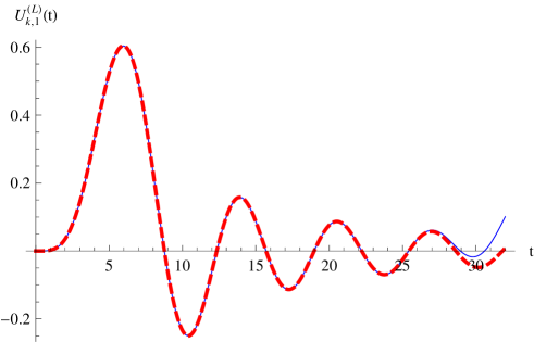
Figure 1: (Color online) Approximation with a single Bessel function ($m=0$ in Eq.(13), dashed red line) of $U^{(L)}_{k,1}(t)$ (continuous blue line) for $k=5,N_{L}=20$

Each additional term in (13) increases the range of $t$ where the Bessel approximation is valid by $N_{L}$. E.g., with $N_{L}=20,k=5$, adding two more Bessel functions (terms $m=\pm 1$) we get the continuation of the plot in Fig.1, with a visible deviation of the approximation from the exact result only at $t\gtrsim 65$ (see Fig. 2). Physically, these terms correspond to waves reflected from the right and left edges, which explains their irrelevance for times when the spin waves have not yet reached the corresponding boundaries.

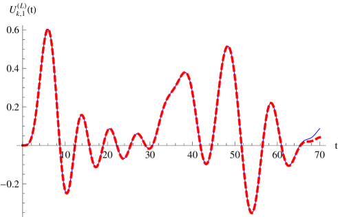
Figure 2: (Color online) Approximation with three Bessel functions ($m=-1,0,1$ in Eq.(13), dashed red line) of $U^{(L)}_{k,1}(t)$ (continuous blue line) for $k=5,N_{L}=20$

II.3 Semiclassical propagator: WKB approximation

In section II.4 we will attempt to obtain a closed analytical formula for the time dependent polarization. In order to do so, another simplification of $U_{k,1}^{(L)}$ is in order. In fact, the leading term $m=0$ in (13), that gives $U^{(L)}_{k,1}(t)=\frac{2\left(-i\right)^{k-1}}{t}kJ_{k}(t)$, valid for $t\lesssim N_{L}$, lends itself to further approximation. From M.Abramowitz and A.Stegun (1970) (leading term of 9.3.15), we can obtain a “WKB approximation” for the Bessel function,

$$J_{k}^{WKB}(t) = \sqrt{\frac{2}{\pi}}\frac{1}{\sqrt[4]{t^{2}-k^{2}}}\cos\left(\phi_{k}(t)\right)\mbox{ for }k<t,$$ (15)

$$\phi_{k}(t) = k\arccos\left(\frac{k}{t}\right)-\sqrt{t^{2}-k^{2}}+\frac{\pi}{4}~{}.$$ (16)

This approximation is commonly called the Debye approximation Weisstein . The name “WKB approximation” is motivated by the fact that the Bessel function is approximated by a sum of two exponential functions with slowly varying amplitude and phase, in close analogy to the well-known WKB approximation method. The corresponding approximation of $U_{k,1}^{(L)}(t)$ can also be obtained from a semiclassical solution of the Schrödinger equation, i.e. a Van Vleck propagator. This will be presented in III.3.3 for circular chains. The WKB approximation breaks down near the classical turning point, which corresponds here to $k=t$ (see Fig.3). For $k>t$, $\phi_{k}(t)$ becomes complex and Eq.(15) has to be replaced by an exponentially decaying function. In the vicinity of the turning point, a uniform approximation is called for which interpolates smoothly between the two regimes.

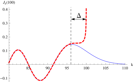
Figure 3: (Color online) Comparison of exact Bessel function (continuous blue line) and its “WKB approximation” (dashed red line), Eq.(15)

Bessel functions can be approximated near the turning point by an Airy function (M.Abramowitz and A.Stegun (1970): 9.3.23),

$$J_{k}(t)\approx\left(\frac{2}{t}\right)^{\frac{1}{3}}Ai(-z),~{}z=\left(\frac{2}{t}\right)^{\frac{1}{3}}(t-k)~{}.$$ (17)

This allows to determine precisely the domain in which the WKB approximation is valid, and where it is not. Fig. 3 shows the comparison for $t=100$ between exact Bessel function and its WKB approximation. The two plots practically coincide up to the last maximum of $J_{k}(t)$ as function of $k$, observed at $k_{m}=t-\Delta$. After that the WKB approximation tends to infinity like $(t-k)^{-\frac{1}{4}}$ whereas the exact $J_{k}(t)$ quietly goes to zero. The maximal allowed approach of $k$ to $t$ in the WKB estimate is given by the position of the last maximum of the Airy function $Ai(-z)$ which takes place at $z_{m}=1.01879$ and is equal to $Ai(-z_{m})=0.535$. The width of the “bad” region where WKB is senseless is thus given by $\Delta=t-k_{m}=\left(\frac{t}{2}\right)^{\frac{1}{3}}z_{m}\approx 0.8t^{\frac{1}{3}}$. It grows with time, but slowly compared to $t$.

II.4 Mean polarization

The total polarization of the chain is defined as $\displaystyle P^{(L)}=\sum_{k=1}^{N_{L}-1}Z_{k}$. In a basis state $\left|\Lambda_{k}\right\rangle$, we have the mean polarization $\left\langle\Lambda_{k}\right|P^{(L)}\left|\Lambda_{k}\right\rangle=N_{L}-2k$. If we put the system initially in the state $\left|\Lambda_{1}\right\rangle$, we obtain the time dependent mean polarization

$$\langle P^{(L)}\left(t\right)\rangle = \sum_{k=1}^{N_{L}-1}\left(N_{L}-2k\right)\left|U_{k,1}^{(L)}(t)\right|^{2}~{}.$$ (18)

Now let us substitute the WKB approximation of the propagator into the expression of the mean polarization. We are allowed to do so only in the “good” interval where the summands are smooth functions of $k$ and the sums can be approximated by integrals. Neglecting the exponentially small terms for $k\geq t$, we are thus led to

$$\left\langle P_{WKB}^{(L)}(t)\right\rangle = \sum_{k<t}(N_{L}-2k)\left|U^{(L)}_{k,1}(t)\right|^{2}$$ (19)

$$= \sum_{k=1}^{[t-\Delta]}(N_{L}-2k)\left|U^{(L)}_{k,1}(t)\right|^{2}$$

$$+\sum_{k=[t-\Delta]}^{[t]}(N_{L}-2k)\left|U^{(L)}_{k,1}(t)\right|^{2}$$

$$= \frac{8}{\pi t^{2}}\sum_{k=1}^{[t-\Delta]}\frac{k^{2}(N_{L}-2k)}{\sqrt{t^{2}-k^{2}}}\frac{1+\cos[2\phi_{k}(t)]}{2}$$

$$+\sum_{k=[t-\Delta]}^{[t]}(N_{L}-2k)\left|U_{k,1}(t)\right|^{2}$$

$$\simeq \frac{4}{\pi t^{2}}\int_{0}^{t}(N_{L}-2k)\frac{k^{2}}{\sqrt{t^{2}-k^{2}}}dk$$

$$-\frac{4}{\pi t^{2}}\int_{t-\Delta}^{t}(N_{L}-2k)\frac{k^{2}}{\sqrt{t^{2}-k^{2}}}dk$$

$$+\frac{4}{\pi t^{2}}\sum_{k=1}^{[t-\Delta]}\frac{k^{2}(N_{L}-2k)}{\sqrt{t^{2}-k^{2}}}\cos(2\phi_{k}(t))$$

$$+\sum_{k=[t-\Delta]}^{[t]}(N_{L}-2k)\left|U^{(L)}_{k,1}(t)\right|^{2}~{},$$

where $[x]$ denotes the integer part of $x$. The first integral in (19) is proportional to $t$,

$$\left\langle P_{WKB}^{(L)}(t)\right\rangle\simeq N_{L}-\frac{16t}{3\pi}~{}.$$ (20)

Let us make an estimate of the remaining terms. The second integral $\frac{1}{t^{2}}\int_{t-\Delta}^{t}\ldots$ is of the order $\sqrt{t\Delta}\approx t^{2/3}$ which is small compared to $t$ when $t\rightarrow\infty$. The sum containing $\cos\left[2\phi_{k}(t)\right]$ contains many summands of both signs which mutually almost cancel and can be neglected (rigorous estimates can be made using the Poisson summation formula). Finally, the last sum can be estimated as the number of summands $\Delta\propto t^{1/3}$, times the maximal value of the summand $(N_{L}-2t)\left[2\left(\frac{2}{t}\right)^{1/3}Ai(-z_{m})\right]^{2}\propto t^{1/3}$. The result is again $\propto t^{2/3}$ and can again be neglected compared to $t$ when $t$ is very large.

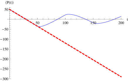
Figure 4: (Color online) Comparison of mean polarizations: exact result (Eq.(18), continuous blue line) versus linear term of WKB approximation (Eq.(20), dashed red line), for $N_{L}=50$

Thus the estimates for the relative errors decay like $t^{-1/3}$ as $t\rightarrow\infty$, and Eq.(20) is therefore the leading behavior of the WKB approximation. While this approximation is rather crude, it nevertheless shows very good agreement with the exact result for times small enough not to allow spin waves to reach the end of the chain. E.g., for $N_{L}=50$ and $t=40$ the Bessel representation (which is basically exact here), gives $P(t)=-17.922$ whereas the WKB result is $N_{L}-\frac{16}{3\pi}t=-17.9601$, i.e. reproduces the Bessel result with 3 digits. In Fig.4 we compare the exact mean polarization (18) with its semiclassical approximation (20) for a chain of $50$ spins. From Eq.(20) we read off a constant rate of spin flips (corresponding here to the speed of propagation of a single spin-wave front) for times $t\apprle N_{L}$, $\left|v^{(L)}\right|=\frac{16}{3\pi}$.

III Circular chain

There are several ways of closing the linear chain (1) of $N_{L}$ spins to a ring:

1. By identification of $S_{N_{L}+1}$ and $S_{1}$: in this system $S_{2},\ldots,S_{N_{L}}$ are subject to spin flipping (see Eq.(21) below);

2. By identification of $S_{N_{L}+1}$ and $S_{1}$ and introduction of an additional interaction term containing $X_{1}$ in (1) that allows $S_{1}$ to flip: in this system $S_{1},\ldots,S_{N_{L}}$ are subject to spin flipping (see Eq.(34) below);

3. By introducing a different coupling between the first spins and the last spins of the linear chain: in section III.3, we will introduce a particular four-spin coupling between $S_{N_{L}-1},S_{N_{L}},S_{1},S_{2}$ .

We will now investigate the dynamics in these different chains. $S_{1}$ will designate always the spin chosen as the reference spin from which all the others are numbered (from $S_{2}$ to $S_{N_{L}}$ turning clockwise on the chains).

III.1 Closing by identification of spins $S_{N_{L}+1}$ and $S_{1}$

The simplest way of closing a linear chain consists in identifying the first and the last spin. When we talk about circular chains we will call the number of spins $N_{C}$. For the present subsection we consider $N_{C}=N_{L}$, such that $S_{N_{C}+1}=S_{1}$. This imposes a corresponding boundary condition on the wave function, but also implies an extra term in the hamiltonian since identifying $S_{1}$ with $S_{N_{C}+1}$ allows to flip spin $S_{N_{C}}$ depending on the state of $S_{N_{C}-1}$ and $S_{N_{C}+1}=S_{1}$. Thus we have to add the term $k=N_{C}$ to $H_{1}^{(L)}$, i.e.

$$H_{1}^{(C)}=\frac{1}{4}\sum_{k=2}^{N_{C}}X_{k}\left(1_{k-1}\otimes 1_{k+1}-Z_{k-1}\otimes Z_{k+1}\right).$$ (21)

Note that $S_{1}$ still never flips as there is no term containing $X_{1}$. In section III.2 we will consider the situation of complete rotational symmetry implemented already on the level of the hamiltonian, where the introduction of yet another flip term also allows $S_{1}$ to flip. The system described by Eq.(21) evolves inside a subspace whose $N_{C}(N_{C}-1)/2$ basis states $\left|\chi_{I,J}\right\rangle$ ($I\in[1,N_{C}-1]$ and $J\leq I$) can be arranged in the form of a triangle,

$$\left|\chi_{1,1}\right\rangle$$

$$\left|\chi_{2,1}\right\rangle,\left|\chi_{2,2}\right\rangle$$

$$\left|\chi_{3,1}\right\rangle,\left|\chi_{3,2}\right\rangle,\left|\chi_{3,3}\right\rangle$$

$$\vdots\hskip 90.0pt\ddots$$

$$\left|\chi_{N_{C}-1,1}\right\rangle,~{}\ldots\ldots\ldots~{},\left|\chi_{N_{C}-1,N_{C}-1}\right\rangle~{}.$$ (22)

We define $\left|\chi_{I,J}\right\rangle$ as the state containing $I$ consecutive spins down (all the others are up), with $J-1$ spins down at the left of $S_{1}$, $S_{1}$ down, and $I-J$ spins down at the right of $S_{1}$ (imagine $S_{1}$ at the top of the chain). For instance, $\left|\chi_{1,1}\right\rangle=\left|\downarrow_{1}\uparrow_{2}\ldots\uparrow_{N_{C}}\right\rangle$, $\left|\chi_{2,1}\right\rangle=\left|\downarrow_{1}\downarrow_{2}\uparrow_{3}\ldots\uparrow_{N_{C}}\right\rangle$, $\left|\chi_{2,2}\right\rangle=\left|\downarrow_{1}\uparrow_{2}\ldots\uparrow_{N_{C}-1}\downarrow_{N_{C}}\right\rangle$, $\left|\chi_{3,1}\right\rangle=\left|\downarrow_{1}\downarrow_{2}\downarrow_{3}\uparrow_{4}\ldots\uparrow_{N_{C}}\right\rangle$, $\left|\chi_{3,2}\right\rangle=\left|\downarrow_{1}\downarrow_{2}\uparrow_{3}\ldots\uparrow_{N_{C}-1}\downarrow_{N_{C}}\right\rangle$, $\left|\chi_{3,3}\right\rangle=\left|\downarrow_{1}\uparrow_{2}\ldots\uparrow_{N_{C}-2}\downarrow_{N_{C}-1}\downarrow_{N_{C}}\right\rangle$, etc.

$H_{1}^{(C)}$ couples a state $\left|\chi_{I,J}\right\rangle$ to at most four neighbors in the triangle: the one above, the one above to the left, the one below, and the one below to the right. Depending on the region in the triangle, not all four of the states exist. A state is coupled to exactly those of the four states that do exist. In order to obtain a matrix representation of $H_{1}^{(C)}$, we order the states $\left|\chi_{I,J}\right\rangle$ in the order $\left|\chi_{1,1}\right\rangle,\left|\chi_{2,1}\right\rangle,\left|\chi_{2,2}\right\rangle,\left|\chi_{3,1}\right\rangle\ldots$, i.e. we introduce a single label $L(I,J)=I(I-1)/2+J$. Therefore, top state $1$ couples to states $\left\{2,3\right\}$ , lower left hand corner state $L=\frac{(N_{C}-1)(N_{C}-2)}{2}+1$ couples to state $L-N_{C}+2$, lower right hand corner state $L=\frac{(N_{C}-1)(N_{C}-2)}{2}+N_{C}-1$ couples to state $L-N_{C}+1$, left border states $L=\frac{I(I-1)}{2}+1$ with $I\in\left[2,N_{C}-2\right]$ couple to states $\left\{L-I+1,L+I,L+I+1\right\}$, right border states $L=\frac{I(I-1)}{2}+I$ with $I\in\left[2,N_{C}-2\right]$ couple to states $\left\{L-I,L+I,L+I+1\right\}$, base states $L=\frac{(N_{C}-1)(N_{C}-2)}{2}+J$ with $J=\left[2,N_{C}-2\right]$ couple to states $\left\{L-N_{C}+1,L-N_{C}+2\right\}$, and inside states $L=\frac{I(I-1)}{2}+J$ with $I\in\left[3,N_{C}-2\right]$ and $1<J<I$ couple to states $\left\{L-I,L-I+1,L+I,L+I+1\right\}$. For example, the matrix representation of $H_{1}^{(C)}$ for $N_{C}=5$ ($\frac{N_{C}(N_{C}-1)}{2}=10$ basis states) reads

$$H_{1}^{(C)}=\frac{1}{2}\left(\begin{array}[]{cccccccccc}0&1&1&0&0&0&0&0&0&0\\ 1&0&0&1&1&0&0&0&0&0\\ 1&0&0&0&1&1&0&0&0&0\\ 0&1&0&0&0&0&1&1&0&0\\ 0&1&1&0&0&0&0&1&1&0\\ 0&0&1&0&0&0&0&0&1&1\\ 0&0&0&1&0&0&0&0&0&0\\ 0&0&0&1&1&0&0&0&0&0\\ 0&0&0&0&1&1&0&0&0&0\\ 0&0&0&0&0&1&0&0&0&0\\ \end{array}\right)~{}.$$ (33)

The general structure of the matrix corresponding to a system of $N_{C}$ spins can be easily derived. The matrix is real and symmetric, and we need to consider only the upper right triangle $(H_{1}^{(C)})_{L,L^{\prime}}$ with $L^{\prime}>L$. To fill this part of the matrix we have to know for a state of the basis to which state below in the triangle (III.1) it is connected. Each state from the first line to the last but one of the triangle is only connected to two consecutive states below it in the triangle (the state directly below and the one below to the right). Therefore, in each line of the upper right part of $H_{1}^{(C)}$ there are only two consecutive non zero elements. Given two states $\chi_{L}$ and $\chi_{L+1}$ of a same line of the triangle, there is one common state among the states coupled to $\chi_{L}$ and the ones coupled to $\chi_{L+1}$. That explains that we observe staircase-structures extending over $1,2,3,\ldots$ rows . Since there are $N_{C}-1$ lines in (III.1) and each line with the exception of the last one gives rise to a staircase, there are altogether $N_{C}-2$ staircases. From one staircase structure to the next, there is a shift of one line and one column, since the first state of a line is not connected to the last state of the preceding one.

A brief remark is in order about the global structure of the distribution of non-zero elements over the matrix. Let us consider for each staircase-structure the first element, i.e. $(H_{1}^{(C)})_{1,2}$, $(H_{1}^{(C)})_{2,4}$, $(H_{1}^{(C)})_{4,7}$, $\ldots$  The coordinates (line, column) of these elements are given by the index $L$ for the elements of the left border in (III.1), $X_{I}=L=\frac{I(I-1)}{2}+1$, and the element below it, $Y_{I}=X_{I}+I=\frac{I(I+1)}{2}+1$. If we plot the $(X_{I},Y_{I})$ points in a plan, we obtain a line whose slope $\frac{Y_{I+1}-Y_{I}}{X_{I+1}-X_{I}}=1+\frac{1}{I}$ converges for $I\rightarrow\infty$ to $1$. This means that for $N_{C}\gg 1$, the matrix representation of $H_{1}^{(C)}$ is very close to a matrix having four non zero diagonals parallel to the main diagonal, but a final curvature of the “off-diagonals” remains for all finite $I$. In the next section we see that straight lines of off-diagonal matrix elements over the entire matrix, parallel to the main diagonal, are obtained with the second way of closing the chain. Lacking a viable analytical technique for diagonalizing $H_{1}^{(C)}$, we diagonalize the hamiltonian numerically, and derive the propagator. The results will be compared to those of the linear chain in section IV.

III.2 Completely periodic chain

Another way of closing the system is to impose periodic boundary conditions $S_{N_{C}+k}=S_{k}$, $k\in\left[1,N_{C}\right]$. This amounts to subjecting also $S_{1}$ to flip by adding an additional flip term $X_{1}$ controlled by $S_{N_{C}}$ and $S_{2}$. The hamiltonian of this system thus reads

$$H_{2}^{(C)} = \frac{1}{4}\sum_{k=1}^{N_{C}}X_{k}\left(1_{k-1}\otimes 1_{k+1}-Z_{k-1}\otimes Z_{k+1}\right)~{}.$$ (34)

The physical important point is that in this system $S_{1}$ is flipped if its nearest-neighbors are of opposite signs ($S_{N_{C}}$ and $S_{2}$), whereas in section III.1, $S_{1}$ is never subjected to spin flipping and always remains in its initial down state. As a consequence, the number of basis states that are dynamically accessible is doubled. Indeed, allowing $S_{1}$ to be flipped, gives access to basis states related to the $\left|\chi_{L}\right\rangle$ by flipping all spins. They form an ensemble of states having $k$ consecutive spins down ($k\in\left[1,N_{C}-1\right]$), where in addition, for each $k\in\left[1,N_{C}-1\right]$, we have the freedom of choosing the starting point of the sequence of flipped spins among the $N_{C}$ spins. So the dimension of the accessible Hilbert space is now $N_{C}(N_{C}-1)$.

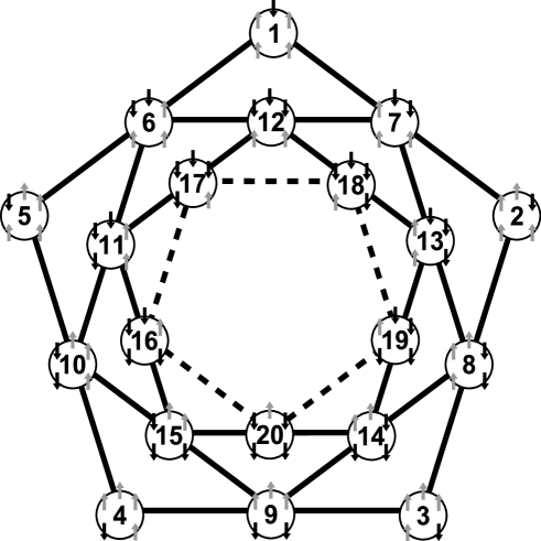
Figure 5: (Color online) Coupling of states introduced by $H_{2}^{(C)}$, Eq.(34), for $N_{C}=5$

It is interesting to note that the couplings between the basis states can be obtained by arranging the states on the vertices of $(N_{C}-1)$ nested $N_{C}$-sided polygons as can be observed in Fig.5 for $N_{C}=5$. A full line represents the coupling between two states. We label the states as can be seen in Fig.5: we follow a polygon until all of its states have been accounted for. Then we move to the next polygon further inside by moving to its first vertex on the center of the last link of the previous polygon, and so on. Using this numbering, we obtain a matrix representation of $H_{2}^{(C)}$, with a simple structure. For example for $N_{C}=4$ we obtain

$$H_{2}^{(C)}=\frac{1}{2}\left(\begin{array}[]{cccccccccccc}0&0&0&0&1&1&0&0&0&0&0&0\\ 0&0&0&0&0&1&1&0&0&0&0&0\\ 0&0&0&0&0&0&1&1&0&0&0&0\\ 0&0&0&0&1&0&0&1&0&0&0&0\\ 1&0&0&1&0&0&0&0&1&1&0&0\\ 1&1&0&0&0&0&0&0&0&1&1&0\\ 0&1&1&0&0&0&0&0&0&0&1&1\\ 0&0&1&1&0&0&0&0&1&0&0&1\\ 0&0&0&0&1&0&0&1&0&0&0&0\\ 0&0&0&0&1&1&0&0&0&0&0&0\\ 0&0&0&0&0&1&1&0&0&0&0&0\\ 0&0&0&0&0&0&1&1&0&0&0&0\\ \end{array}\right)~{}.$$ (47)

The general structure corresponding to a system of $N_{C}$ spins can again be easily derived. Since the matrix is real and symmetric, we need to consider only the upper right triangle $(H_{2}^{(C)})_{L,L^{\prime}}$ with $L^{\prime}>L$. We observe two neighboring off-diagonals, parallel to the main diagonal, and a few non zero elements next to the (vanishing) main diagonal. The non zero terms directly next to the main diagonal are the elements $(H_{2}^{(C)})_{kN_{C},kN_{C}+1}$ with $k\in\left[1,N_{C}-2\right]$. The first diagonal extends from $(H_{2}^{(C)})_{1,N_{C}+1}$ to $(H_{2}^{(C)})_{N_{C}(N_{C}-2),N_{C}(N_{C}-1)}$ (all elements equal to one), the second diagonal goes from $(H_{2}^{(C)})_{1,N_{C}+2}$ to $(H_{2}^{(C)})_{N_{C}(N_{C}-2)-1,N_{C}(N_{C}-1)}$ (all elements equal to one except the $(kN_{C})^{th}$ with $k\in[1,N_{C}-3]$). The fact that the two most straightforward ways of closing the chain lead to a relevant Hilbert space of dimension of ${\cal O}(N_{C}^{2})$ instead of ${\cal O}(N_{L})$, is rather interesting and will be explored further below. At the same time it would be interesting to find out whether there exist other ways of closing the chain that lead to dynamics resembling as closely as possible, the dynamics of the linear chain, and in particular to a relevant Hilbert space of dimension of ${\cal O}(N_{C})$. In the following two subsections we present such a closure and profit from the machinery developed in section II to study the corresponding dynamics.

III.3 Closing by a particular coupling between $S_{N_{C}-1}$, $S_{N_{C}}$, $S_{1}$, and $S_{2}$

We now study a particular way of closing the linear chain for which, as we are going to see, the system evolves in a Hilbert space whose dimension scales only linearly with the size of the chain. We consider a system that has the same nearest-neighbors interactions as $H_{2}^{(C)}$ for spin $S_{2}$ to spin $S_{N_{C}-1}$, and an additional particular coupling for spins $S_{N_{C}-1}$, $S_{N_{C}}$, $S_{1}$ and $S_{2}$ that leads to the following action: if spin $S_{N_{C}-1}$ and spin $S_{2}$ are the same, then spin $S_{N_{C}}$ and spin $S_{1}$ are flipped, otherwise nothing is done. The hamiltonian of such a system is

$$H_{3}^{(C)} = \frac{1}{4}\sum_{k=2}^{N_{C}-1}X_{k}\left(1_{k-1}\otimes 1_{k+1}-Z_{k-1}\otimes Z_{k+1}\right)$$ (48)

$$+\frac{1}{4}X_{N_{C}}X_{1}\left(1_{N_{C}-1}1_{2}+Z_{N_{C}-1}Z_{2}\right)~{}.$$

Note the small difference compared to $H_{2}^{(C)}$. As before, we denote $\left|\chi_{k}\right\rangle=\left|\downarrow_{1}\ldots\downarrow_{k}\uparrow_{k+1}\ldots\uparrow_{N_{C}}\right\rangle=\left|\Lambda_{k}\right\rangle$ the state where spins $S_{1}$ to $S_{k}$ are down and all the others up for $k\in\left[1\,,N_{C}-1\right]$. Then we define $\left|\chi_{N_{C}+k-1}\right\rangle=\left|\uparrow_{1}\ldots\uparrow_{k}\downarrow_{k+1}\ldots\downarrow_{N_{C}}\right\rangle=\left|\overline{\Lambda_{k}}\right\rangle$, $k\in\left[1\,,N_{C}-1\right]$, the state where spins $S_{1}$ to $S_{k}$ are up, all the others down. The $\left|\overline{\Lambda_{k}}\right\rangle$ are the mirror states of $\left|\Lambda_{k}\right\rangle$ in the sense that all spins are flipped. Let us suppose again that the system starts in the state $\left|\chi_{1}\right\rangle=\left|\downarrow_{1}\uparrow_{2}\ldots\uparrow_{N_{C}}\right\rangle$. This state couples to $\left|\chi_{2}\right\rangle=\left|\downarrow_{1}\downarrow_{2}\uparrow_{3}\ldots\uparrow_{N_{C}}\right\rangle$ and $\left|\chi_{2(N_{C}-1)}\right\rangle=\left|\uparrow_{1}\uparrow_{2}\ldots\uparrow_{N_{C}-1}\downarrow_{N_{C}}\right\rangle$. For general $k\in\left[2\,,N_{C}-2\right]$, $\left|\chi_{k}\right\rangle$ couples to $\left|\chi_{k-1}\right\rangle$ and $\left|\chi_{k+1}\right\rangle$ and $\left|\chi_{N_{C}+k-1}\right\rangle=\left|\overline{\Lambda_{k}}\right\rangle$ couples to $\left|\overline{\Lambda_{k-1}}\right\rangle$ and $\left|\overline{\Lambda_{k+1}}\right\rangle$. Thus, at the end of the chain, the system branches over into the mirror states, which in turn lead back to the original states and therefore give rise to a closed basis of $2(N_{C}-1)$ states. We note, however, that neither the state with all spins up nor the state with all spins down is any longer an eigenstate of $H_{3}^{(C)}$, with consequences for the spin amplification discussed in Sec.IV. The matrix of the hamiltonian in the basis of the $\left|\chi_{k}\right\rangle$, for $k\in\left[1,2(N_{C}-1)\right]$ is

$$H_{3}^{(C)}=\frac{1}{2}\left(\begin{array}[]{ccccccc}0&1&0&\ldots&\ldots&0&1\\ 1&0&1&\ddots&{}\hfil&{}\hfil&0\\ 0&1&0&\ddots&\ddots&{}\hfil&\vdots\\ \vdots&\ddots&\ddots&\ddots&\ddots&\ddots&\vdots\\ \vdots&{}\hfil&\ddots&\ddots&0&1&0\\ 0&{}\hfil&{}\hfil&\ddots&1&0&1\\ 1&0&\ldots&\ldots&0&1&0\\ \end{array}\right)~{}.$$ (56)

This is a well-known hamiltonian of a regular chain closed into a ring. Its eigenvalues and eigenvectors are given by

$$\lambda_{p}^{(C)}=\cos[\frac{p\,\pi}{N_{C}-1}]\mbox{ and }$$

$$\left|\Phi_{p}^{(C)}\right\rangle=\frac{1}{\sqrt{2(N_{C}-1)}}\sum_{k=1}^{2(N_{C}-1)}e^{i\frac{p\pi k}{N_{C}-1}}\left|\chi_{k}\right\rangle$$ (57)

for $p\in\left[1,2(N_{C}-1)\right]$. Finally, we obtain the expression of the propagator

$$U_{k,k_{0}}^{(C)}\left(t\right) = \left\langle\chi_{k}\right|e^{-iH_{3}^{(C)}t}\left|\chi_{k_{0}}\right\rangle$$ (58)

$$= \sum_{p=1}^{2(N_{C}-1)}\left\langle\chi_{k}\right|\left.\Phi^{(C)}_{p}\right\rangle e^{-it\lambda_{p}^{(C)}}\left\langle\Phi^{(C)}_{p}\right|\left.\chi_{k_{0}}\right\rangle$$

$$= \sum_{p=1}^{2(N_{C}-1)}F^{(C)}_{k,k_{0}}(p\,,t)$$

with $F^{(C)}_{k,k_{0}}(p\,,t)\equiv\frac{1}{2(N_{C}-1)}e^{i\frac{p\pi(k-k_{0})}{N_{C}-1}}e^{-it\cos\frac{p\pi}{N_{C}-1}}~{}.$

III.3.1 Representation of the propagator in terms of Bessel functions

Using that $F^{(C)}_{k,k_{0}}(p\ +2(N_{C}-1)\,,t)=F^{(C)}_{k,k_{0}}(p\,,t)$, we can use the Poisson summation formula to find

$$U_{k,k_{0}}^{(C)}\left(t\right) = \sum_{m=-\infty}^{\infty}\int_{0}^{2(N_{C}-1)}e^{2i\pi mp}F^{(C)}_{k,k_{0}}(p\,,t)\,dp$$ (59)

$$= \sum_{m=-\infty}^{\infty}(-i)^{k-k_{0}+2m(N_{C}-1)}J_{k-k_{0}+2m(N_{C}-1)}(t)~{}.$$

For the special case where the system starts in the state $\left|\chi_{1}\right\rangle$, we obtain

$$U_{k,1}^{(C)}\left(t\right) = (-i)^{k-1}\sum_{m=-\infty}^{\infty}(-1)^{m(N_{C}-1)}J_{k-1+2m(N_{C}-1)}\left(t\right).$$ (60)

III.3.2 Semiclassical propagator for small times ( $t<N_{c}-1$)

The Bessel function vanishes exponentially fast if its index is large and exceeds its argument. Therefore the infinite sum (60) reduces in fact to only a few summands significantly different from zero. In particular, if $t<N_{c}-1$ only a single term corresponding to $m=0$ or $m=-1$ survives respectively for $1\leq k\leq N_{c}-1$ (states $\Lambda$) and $N_{c}\leq k\leq 2(N_{c}-1)$ (states $\overline{\Lambda}$),

$$U_{k,1}^{(C)}(t)\approx(-i)^{k-1}J_{k-1}(t)\mbox{, }\,\,\,1\leq k\leq N_{c}-1;$$

$$U_{k,1}^{(C)}(t)\approx(-1)^{N_{C}-1}(i)^{k-1}J_{2N_{c}-k-1}(t)\mbox{, }\,\,\,N_{c}\leq k\leq 2(N_{c}-1)\,.$$

If $1\ll k$ (respectively $1\ll 2N_{c}-k-1$), these Bessel functions can be replaced by their WKB approximation (15).

III.3.3 Van Vleck approach

Before considering the polarization dynamics, we present an alternative and more physical approach for calculating the semiclassical propagator for $k\in\left[1,N_{C}-1\right]$ and $k<t+1$. The same problem as before can be approached by deriving the classical hamiltonian associated to the system; the method and its generalization to chains with slowly changing parameters are described in the review Braun (1993). The action of $H_{3}^{(C)}$ on a basis state, $H_{3}^{(C)}\left|\chi_{k}\right\rangle=\frac{1}{2}\left(\left|\chi_{k-1}\right\rangle+\left|\chi_{k+1}\right\rangle\right)$, can be rewritten in terms of shift operators, if we upgrade the index $k$ to a continuous variable, i.e. $H_{3}^{(C)}\left|\chi(k)\right\rangle=\frac{1}{2}\left(\left|\chi(k-1)\right\rangle+\left|\chi(k+1)\right\rangle\right)=\frac{1}{2}\left(e^{-\partial/\partial_{k}}\left|\chi(k)\right\rangle+e^{\partial/\partial_{k}}\left|\chi(k)\right\rangle\right)$. This is a reasonable approach in the limit of very long chains, $N_{C}\rightarrow\infty$, which can be considered the classical limit. If we denote $\phi=-i\partial/\partial_{k}$ the momentum canonically conjugate to the coordinate $k$, we can write $H_{3}^{(C)}\left|\chi(k)\right\rangle=\frac{1}{2}\left(e^{-i\phi}+e^{i\phi}\right)\left|\chi(k)\right\rangle=\cos\left(\phi\right)\left|\chi(k)\right\rangle$. In the classical limit we therefore obtain a corresponding classical hamiltonian $H_{3}^{Cl}=\cos\left(\phi\right)$. Since $H_{3}^{Cl}$ does not depend on $k$, the momentum is an integral of motion connected with the energy by $E=\mbox{cte}=\cos(\phi)$. The trajectory of the motion follows from the canonical equation $\dot{k}(t)=\frac{\partial H_{3}^{Cl}}{\partial\phi}=-\sin(\phi)$, hence $k(t)=k_{0}-t\sin(\phi)$. The classical action is given by $\displaystyle S(k,k_{0},t)=\int_{k_{0}}^{k}\phi(\tilde{k})d\tilde{k}-E(k,k_{0},t)t=(k-k_{0})\phi-E(k,k_{0},t)t$. We find two classical paths, $\phi_{1}(k,k_{0},t)=-\arcsin(\frac{k-k_{0}}{t})$ and $\phi_{2}(k,k_{0},t)=\pi+\arcsin(\frac{k-k_{0}}{t})$. Their associated classical energies are $E_{1}(k,k_{0},t)=\cos(\phi_{1}(k,k_{0},t))=\frac{1}{t}\sqrt{t^{2}-(k-k_{0})^{2}}$ and $E_{2}(k,k_{0},t)=\cos(\phi_{2}(k,k_{0},t))=-\frac{1}{t}\sqrt{t^{2}-(k-k_{0})^{2}}$. Finally, the associated classical actions are given by $S_{1}(k,k_{0},t)=(k-k_{0})\phi_{1}(k,k_{0},t)-E_{1}(k,k_{0},t)t=-(k-k_{0})\arcsin(\frac{k-k_{0}}{t})-\sqrt{t^{2}-(k-k_{0})^{2}}$ and $S_{2}(k,k_{0},t)=(k-k_{0})\phi_{2}(k,k_{0},t)-E_{2}(k,k_{0},t)t=(k-k_{0})(\pi+\arcsin(\frac{k-k_{0}}{t}))+\sqrt{t^{2}-(k-k_{0})^{2}}$. The semiclassical Van Vleck propagator is obtained by summing over all the classical paths,

$$U^{VV}_{k,k_{0}}(t)=\sum_{\alpha}\sqrt{\frac{1}{2i\pi}\left|\frac{\partial^{2}S_{\alpha}}{\partial k\partial k_{0}}\right|}\exp(i\left(S_{\alpha}(k,k_{0},t)-\nu_{\alpha}\frac{\pi}{2}\right))~{},$$ (61)

where $\nu_{\alpha}$ is the Morse index for the classical path $\alpha$. For the case of the small times considered we have only two classical paths with $\nu_{1}=-1$ and $\nu_{2}=0$ and therefore,

$$U^{VV}_{k,k_{0}}(t)=U^{VV,(1)}_{k,k_{0}}(t)+U^{VV,(2)}_{k,k_{0}}(t)$$ (62)

$$U^{VV,(1)}_{k,k_{0}}(t)=\sqrt{\frac{i}{2\pi\sqrt{t^{2}-(k-k_{0})^{2}}}}\exp(-iX)$$

$$U^{VV,(2)}_{k,k_{0}}(t)=\sqrt{\frac{1}{2i\pi\sqrt{t^{2}-(k-k_{0})^{2}}}}(-1)^{k-k_{0}}\exp(iX)$$

with $X=(k-k_{0})\arcsin(\frac{k-k_{0}}{t})+\sqrt{t^{2}-(k-k_{0})^{2}}$. It can be easily checked that (62) with $k_{0}=1$ is exactly the same as $U^{WKB}_{k,1}(t)^{(C)}=(-i)^{k-1}J^{WKB}_{k-1}(t)$ with $J^{WKB}_{k-1}(t)$ given by (15).

III.3.4 Mean polarization

The operator for the total polarization is now $\displaystyle P^{(C)}=\sum_{k=1}^{2(N_{C}-1)}Z_{k}$. Expressed in the basis of the $\left\{\left|\chi_{k}\right\rangle\right\}$, the mean polarization is $\left\langle\chi_{k}\right|P^{(C)}\left|\chi_{k}\right\rangle=(N_{C}-2k)$ for $k\in[1,N_{C}-1]$, and $\left\langle\chi_{k}\right|P^{(C)}\left|\chi_{k}\right\rangle=-(3N_{C}-2k-2)$ for $k\in[N_{C},2(N_{C}-1)]$. If we put the system initially in the state $\left|\chi_{1}\right\rangle$, we obtain the time dependent mean polarization,

$$\langle P^{(C)}(t)\rangle = \sum_{k=1}^{N_{C}-1}\left(N_{C}-2k\right)\left|U_{k,1}^{(C)}(t)\right|^{2}$$ (63)

$$- \sum_{k=N_{C}}^{2(N_{C}-1)}\left(3N_{C}-2k-2\right)\left|U_{k,1}^{(C)}(t)\right|^{2}$$

As before, the WKB approximation of the mean polarization is obtained by replacing the exact propagator in Eq.(63) by its WKB approximation $U_{k,1}^{WKB}(t)^{(C)}$,

$$\langle P^{(C)}_{WKB}(t)\rangle$$

$$= \sum_{k<t+1}(N_{C}-2k)\left|U^{WKB}_{k,1}(t)^{(C)}\right|^{2}$$

$$- \sum_{k>2(N_{C}-1)-t+1}(3N_{C}-2k-2)\left|U^{WKB}_{k,1}(t)^{(C)}\right|^{2}$$

$$= \sum_{k<t+1}(N_{C}-2k)\left|J^{WKB}_{k-1}(t)\right|^{2}$$

$$- \sum_{k>2(N_{C}-1)-t+1}(3N_{C}-2k-2)\left|J^{WKB}_{2(N_{C}-1)-k+1}(t)\right|^{2}$$

$$= \sum_{k<t+1}(N_{C}-2k)\frac{2}{\pi}\frac{\cos^{2}\left[\phi[k+1,t]\right]}{\sqrt{t^{2}-(k-1)^{2}}}$$

$$- \sum_{k>2(N_{C}-1)-t+1}\frac{2}{\pi}(3N_{C}-2k-2)\frac{\cos^{2}\left[\phi[2(N_{C}-1)-k+1,t]\right]}{\sqrt{t^{2}-\left(2(N_{C}-1)-k+1\right)^{2}}}~{}.$$

Making the same kind of calculation as before and neglecting in the limit $N_{C}\gg 1$ the terms in the vicinity of the turning point (see the discussion about the estimation of remaining terms neglected for the expression of mean polarization in the case of the linear chain in section I.D), we finally obtain for the linear contribution of the mean polarization

$$\left\langle P_{WKB}^{(C)}(t)\right\rangle\simeq(N_{C}-1)-\frac{4t}{\pi}.$$ (64)

We read off a rate of spin flips $\left|v^{(C)}\right|=\frac{4}{\pi}$. It is reduced by $25\%$ compared to the one obtained for the linear chain, $\left|v^{(L)}\right|=\frac{16}{3\pi}$. There are now two propagating wave fronts superposed. Each contributes with about 50% probability, but the additional front propagating to the left has at each time step a smaller number of flipped spins, which explains the reduced total spin-flip rate. We thus have the astonishing result that a single modified coupling at the end of the chain can drastically and macroscopically change the dynamics of the entire chain, even in the limit of arbitrarily long chains. This is a highly unusual situation, as in most physical systems boundary terms are negligible in the thermodynamic limit. Exceptions can exist for systems exactly at a phase transition Braun et al. (1998), but this is clearly not the situation for our spin chains.

In section IV we examine the differences in the dynamics for the three different ways of closing the chain in more detail and elucidate their physical origin. Before doing so, we would like to point out, however, yet another way of closing the chain, with the rather peculiar property of allowing a dynamics corresponding to different topologies of the chain depending on the subspace of Hilbert space considered.

III.4 Existence of a circular chain dynamically equivalent to the linear chain

Consider the situation where spins $S_{2}$ to $S_{N_{C}-2}$ are coupled through the same nearest-neighbor interactions as for $H^{(L)}$, but where we have an additional coupling for spins $S_{N_{C}-2}$, $S_{N_{C}-1}$, $S_{N_{C}}$ and $S_{1}$ that leads to the following action: if spins $S_{N_{C}-2}$ and $S_{1}$ are the same and different from $S_{N_{C}}$, then spin $S_{N_{C}-1}$ is flipped, otherwise nothing is done. The hamiltonian of such a system is given by

$$H^{(C)}_{4} = \frac{1}{4}\sum_{k=2}^{N_{C}-2}X_{k}\left(1_{k-1}\otimes 1_{k+1}-Z_{k-1}\otimes Z_{k+1}\right)$$

$$+ \frac{1}{8}X_{N_{C}-1}\left(1_{N_{C}-2}\otimes 1_{1}+Z_{N_{C}-2}\otimes Z_{1}\right)\left(1_{N_{C}}\otimes 1_{1}-Z_{N_{C}}\otimes Z_{1}\right)\,.$$

In this system the states with all spins up or down are still stationary. One verifies that in the full Hilbert space spanned by the $2^{N_{C}}=2^{N_{L}}$ computational basis states the matrix representations of $H^{(L)}$ and $H^{(C)}_{4}$ differ. Nevertheless, it turns out that the subspaces connected to the initial state $\left|\Lambda_{1}\right\rangle$ through the dynamics generated by $H^{(L)}$ and $H^{(C)}_{4}$ are identical for the two hamiltonians. Furthermore, the matrix representations of $H^{(L)}$ and $H^{(C)}_{4}$ in these parts of Hilbert space connected to $\left|\Lambda_{1}\right\rangle$ are identical, and thus lead to identical dynamics. We therefore have the interesting situation that the different topology of the circular chain manifests itself only in a certain subspace of Hilbert space, whereas within the subspace relevant for the spin amplification problem one cannot distinguish the two hamiltonians through the dynamics which they generate, whatever the observable.

IV Comparison of linear chain and circular chains

In the following subsections we compare the time evolution of the total polarizations as well as the total fidelities with respect to the two initial states of the first spin for the different hamiltonians presented above. We define the total fidelities $F^{(X)}(t)$ ($X\in\left\{L,C1,C2,C3\right\}$) for $H^{(L)}$, $H_{1}^{(C)}$, $H_{2}^{(C)}$ and $H_{3}^{(C)}$, as

$$F^{(X)}(t) = F_{0}^{(X)}(t)+F_{1}^{(X)}(t)\mbox{ with}$$ (66)

$$F_{0}^{(X)}(t) = \langle\Lambda_{0}(t)|\left(\sum_{m=1}^{N_{X}}|\uparrow_{m}\rangle\langle\uparrow_{m}|\right)|\Lambda_{0}(t)\rangle$$

$$F_{1}^{(X)}(t) = \langle\Lambda_{1}(t)|\left(\sum_{m=1}^{N_{X}}|\downarrow_{m}\rangle\langle\downarrow_{m}|\right)|\Lambda_{1}(t)\rangle\,,$$ (67)

with $|\Lambda_{0}(0)\rangle=|\Lambda_{0}\rangle=\left|\uparrow_{1}\ldots\uparrow_{N_{X}}\right\rangle$ and $|\Lambda_{1}(0)\rangle=|\Lambda_{1}\rangle=\left|\downarrow_{1}\uparrow_{2}\ldots\uparrow_{N_{X}}\right\rangle$. These fidelities can be considered as amplification factors summed over the two initial basis states. They are a generalization of the usual fidelity considered in the spin transfer problem, where the fidelity of the state of the final spin with respect to the pure initial states of the first spin are considered Bose (2003). As $H^{(L)}$, $H_{1}^{(C)}$, and $H_{2}^{(C)}$ conserve the basis state $|\Lambda_{0}\rangle$ we will see that for them the total fidelity is directly related to the average total polarization. However, $H_{3}^{(C)}$ does not conserve $|\Lambda_{0}\rangle$. In this situation, the total fidelities are useful for comparing the overall performance of the different devices as spin amplifier. Note that all fidelities have initial value $N_{L}+1$ ($N_{C}+1$), and are bounded from above by $2N_{L}$ ($2N_{C}$) for linear (circular) chains.

IV.1 Comparison of $H^{(L)}$ and $H_{3}^{(C)}$

In Fig.6 we compare the time evolution of the mean polarizations for the linear chain $H^{(L)}$ studied in section II with basis of size $N_{L}-1$, and the circular chain $H_{3}^{(C)}$ studied in section III.3 with basis of size $2(N_{C}-1)$. We first consider the case $N_{C}=N_{L}$. We observe that the mean polarizations for the two types of chains oscillate with approximately the same frequency. For $t\apprle N_{L}$ the mean polarizations decrease linearly, but with a difference in the slopes of $25\%$ as predicted by Eq.(20) and Eq.(64). The question of the physical origin of the different behaviors arises. The simulations shown in Fig.6 were done for $N_{L}=N_{C}=51$.

Adding an additional local term to the hamiltonian for closing the chain would be expected to lead at most to $1/N_{L}\sim 2\%$ effect. Moreover, our analytical results show that the $25\%$ effect persists for $N_{L}\rightarrow\infty$. A first guess about the origin of the different behavior might be the dimension of the involved basis sets. Since the dimension of the basis for $H^{(L)}$ ($\left\{\left|\Lambda_{k}\right\rangle\right\}$ with $k\in[1,N_{L}-1]$, seen in section II.1) is half of the one of $H_{3}^{(C)}$ ($\left\{\left|\Lambda_{k}\right\rangle\right\}$ plus the corresponding mirror states $\left\{\left|\overline{\Lambda_{k}}\right\rangle\right\}$ with $k\in[1,N_{C}-1]$, as seen in section III.3), we might think that this is a reason for the observed difference. In order to check this hypothesis, we recalculated the polarization for the circular chain for $N_{C}=(N_{L}+1)/2$ in which case the two bases have the same dimension. In order to compare the polarization of chains of different length, we subtract the initial polarization, i.e. we consider the change of polarization with respect to the initial state. As Fig.6 shows, we observe the same difference between the slopes of the two mean polarizations as function of time (for $t\apprle N_{L}/2$) as before. Again, this is confirmed by the leading terms in Eq.(20) and Eq.(64), which are independent of $N_{L}$, $N_{C}$. This shows that the difference of basis sizes is not responsible for the different behavior of the two systems. The matrix representations of the two hamiltonians $H^{(L)}$ and $H_{3}^{(C)}$ , Eqs.(7) and (56), differ only by the two off-diagonal matrix elements $H_{1,N_{L}-1}=H_{N_{L}-1,1}$, which equal $1$ for the circular chain, but $0$ for the linear chain. Thus, one would expect at worst a correction of ${\cal O}(N_{L})$ to the eigenvalues and eigenstates of $H_{3}^{(C)}$. This is confirmed by numerical diagonalization, which indicates that the average absolute difference between corresponding matrix elements of the two propagators decays even more rapidly, roughly as $1/N_{L}^{2}$. Clearly, the slightly different matrix representations cannot explain the observed macroscopic differences either. Fig.6 also shows that the mean polarization of the circular chain oscillates approximately twice as fast for $N_{C}=(N_{L}+1)/2$ compared to $N_{C}=N_{L}$. This makes sense, as the oscillation period is set by the time it takes for the spin waves to reach the end of the chain. Also, for $N_{C}=(N_{L}+1)/2$, the amplitude of the signal is roughly half the one for $N_{C}=N_{L}$ since the number of spins of the circular chain has been divided by 2 (up to one spin).

All of this shows that the important difference in the two models lies in the physical structure of the basis functions. The single additional coupling in $H_{3}^{(C)}$ allows access to a new part of Hilbert space (i.e. the additional basis states $\left|\overline{\Lambda_{k}}\right\rangle$). Since the $\left|\overline{\Lambda_{k}}\right\rangle$ have opposite polarization compared to $\left|\Lambda_{k}\right\rangle$, their admixture reduces the total polarization signal compared to the linear chain. Thus, a kind of bifurcation takes place in Hilbert space, depending on the presence of the additional coupling, and the difference in the physical properties of the additionally accessible basis states leads to the macroscopically different behavior.

In Fig.7 we show the total fidelities. For $H^{(L)}$, $F^{(L)}(t)$ behaves like the inverted polarization $\langle P^{(L)}(t)\rangle$, scaled by a factor $1/2$ and shifted by a constant. Indeed we have $F^{(L)}(t)=F_{0}^{(L)}(t)+F_{1}^{(L)}(t)$ with $F_{0}^{(L)}(t)=\frac{N_{L}}{2}+\frac{1}{2}\langle\Lambda_{0}(t)|P^{(L)}|\Lambda_{0}(t)\rangle$ and $F_{1}^{(L)}(t)=\frac{N_{L}}{2}-\frac{1}{2}\langle\Lambda_{1}(t)|P^{(L)}|\Lambda_{1}(t)\rangle$. But since $\left|\Lambda_{0}\right\rangle$ is stationary $F_{0}^{(L)}(t)$ reduces to $N_{L}$, and so

$$F^{(L)}(t)=\frac{3}{2}N_{L}-\frac{1}{2}\langle P^{(L)}(t)\rangle$$ (68)

For $H_{3}^{(C)}$ we observe that the total fidelity immediately deteriorates (whereas $F^{(L)}(t)$ increases initially), and remains much smaller than $F^{(L)}(t)$. This behavior results from $F_{0}^{(C3)}(t)$ which is not constant, as $\left|\Lambda_{0}\right\rangle$ is no longer a stationary state. The dynamics generated by $H_{3}^{(C)}$ starting from $\left|\Lambda_{0}\right\rangle$ evolves apparently in a subspace of dimension $2^{N_{C}-2}$ (verified numerically up to $N_{C}=9$). In order to compare the total fidelities for the different chains on equal footing, all fidelities have been plotted in Fig.7 for chains of 8 spins. Not shown in Fig.7 is that if we wait a sufficiently long time, the total fidelity $F^{(C3)}(t)$ can become large again for particular values of $t$. As an example, for $N_{C}=8$ we obtain $F^{(C3)}(290)\approx 13.09$, close to the maximal possible value 16 for this chain. However, comparisons of the fidelity should be made for a given fixed time interval, as for sufficiently long times a spin-configuration arbitrarily close to a given one can be found Bose (2003).

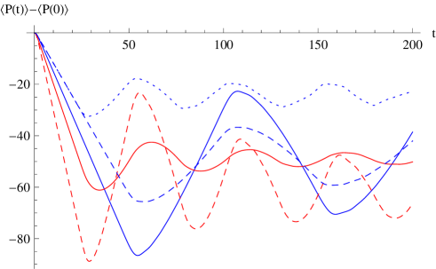
Figure 6: (Color online) Comparison of mean polarizations $\left\langle P(t)\rangle-\langle P(0)\right\rangle$ for linear chain $H^{(L)}$ (continuous blue line), circular chain $H^{(C)}_{3}$ with $N_{C}=N_{L}$ (dashed blue line), circular chain $H^{(C)}_{3}$ with $N_{C}=(N_{L}+1)/2$ (dotted blue line), and circular chains $H_{1}^{(C)}$ (dashed red line), $H_{2}^{(C)}$ (continuous red line) with $N_{C}=N_{L}=51$

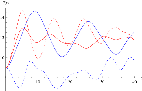
Figure 7: (Color online) Comparison of total fidelities $F(t)$ for linear chain $H^{(L)}$ (continuous blue line), circular chain $H^{(C)}_{3}$ (dashed blue line), and circular chains $H_{1}^{(C)}$ (dashed red line), $H_{2}^{(C)}$ (continuous red line), with $N_{C}=N_{L}=8$

IV.2 Comparison of $H^{(L)}$, $H_{1}^{(C)}$, and $H_{2}^{(C)}$

In Fig.8, Fig.9, and Fig.10, we plot the behavior of mean polarizations $\langle P^{(L)}\rangle$, $\langle P^{(C)}_{1}\rangle$ and $\langle P^{(C)}_{2}\rangle$ for chains of different lengths. For $H_{1}^{(C)}$ and $H_{2}^{(C)}$, the mean polarizations were calculated by numerical diagonalization since generalizing the semiclassical approach to these hamiltonians would be rather cumbersome. For $\langle P^{(L)}\rangle$, $\langle P^{(C)}_{1}\rangle$ and $\langle P^{(C)}_{2}\rangle$ we observe that the slopes of the curves for sufficiently small times, where the mean polarizations behave linearly, are independent of the size of the chains. They equal $\left|v^{(L)}\right|=\frac{16}{3\pi}\approx 1.69$ (obtained analytically, see above) in the case of $H^{(L)}$, $\left|v^{(C)}_{1}\right|\approx 3.39$ and $\left|v^{(C)}_{2}\right|\approx 2.16$ (obtained numerically) in the case of $H^{(C)}_{1}$ and $H^{(C)}_{2}$. Therefore, the polarizations of circular chains $H^{(C)}_{1}$ and $H^{(C)}_{2}$ reach their first minimum respectively about $2$ and $1.28$ times faster than the linear ones.

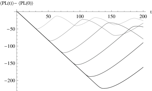
Figure 8: (Color online) Mean polarizations $\langle P^{(L)}(t)\rangle-\langle P^{(L)}(0)\rangle$ for linear chains $H^{(L)}$ for different chain sizes (from $N=30$ (top curve) to $N_{L}=130$ (bottom curve) in steps of $20$)

Figure 9: (Color online) Mean polarizations $\langle P^{(C)}_{1}(t)\rangle-\langle P^{(C)}_{1}(0)\rangle$ for circular chains $H^{(C)}_{1}$ for different chain sizes (from $N=30$ (top curve) to $N_{L}=130$ (bottom curve) in steps of $20$)

Figure 10: (Color online) Mean polarizations $\langle P^{(C)}_{2}(t)\rangle-\langle P^{(C)}_{2}(0)\rangle$ for circular chains $H^{(C)}_{2}$ for different chain sizes (from $N=30$ (top curve) to $N_{L}=130$ (bottom curve) in steps of $20$)

Since $\left|\Lambda_{0}\right\rangle$ remains stationary for $H_{1}^{(C)}$ and $H_{2}^{(C)}$, the total fidelities $F^{(C1)}$ and $F^{(C2)}$ follow the same law as Eq.(68) with corresponding mean polarizations (see Fig.7). The origins of the different behaviors compared to $H^{(L)}$ are more complex here. First of all, the dimensions of the set of basis states connected by $H_{1}^{(C)}$, $H_{2}^{(C)}$ and $H^{(C)}_{3}$ already differ in their scaling with the length of the chains (scaling as ${\cal O}(N_{C}^{2})$ for $H_{1}^{(C)}$, $H_{2}^{(C)}$ and as ${\cal O}(N_{C})$ for $H^{(C)}_{3}$). Secondly, the matrix representations are substantially different, and in fact nonequivalent, such that the spectra of the hamiltonians in the accessible Hilbert spaces are different. This can be observed in Fig.11 where we compare the spectra for the different hamiltonians. The size of the different chains have been chosen such that the basis of $H^{(L)}$, $H_{1}^{(C)}$, $H_{2}^{(C)}$ and $H_{3}^{(C)}$ are of same dimension ($7140$ basis states with $N_{L}=7141$, $N_{C1}=120$, $N_{C2}=80$, $N_{C3}=3571$, with $N_{C1}$, $N_{C2}$, $N_{C3}$, the sizes of the circular chains corresponding to $H_{1}^{(C)}$, $H_{2}^{(C)}$ and $H_{3}^{(C)}$). We can observe that the spectra for $H^{(L)}$ and $H_{3}^{(C)}$ roughly coincide, as do the spectra for $H_{1}^{(C)}$ and $H_{2}^{(C)}$. For $H^{(L)}$ and $H_{3}^{(C)}$ we have seen in subsections II.1 and III.3 that the energy levels are given by a 1D tight-binding model with nearest-neighbors hopping, and thus follow the cosine laws in Eq.(9) and Eq.(III.3). For $H_{1}^{(C)}$, $H_{2}^{(C)}$ we have in the limit of large $N_{C}$ for most states essentially a 2D tight-binding model: All states inside the pyramid Eq.(III.1) are coupled to four nearest neighbors, and the same is true for the states on the vertices of all polygons in Fig.5 for $H_{2}^{(C)}$, with the exception of the innermost and the outermost polygons. However, the spectra differ substantially here from the usual $\cos(k_{x})+\cos(k_{y})$ spectra for a tight-binding model on a square lattice due to the unusual geometry. For example, for $N_{C}=5$, the lattice corresponding to $H_{2}^{(C)}$ has the dihedral symmetry of a pentagon ($C_{5v}$, see Fig. 5). This symmetry leads to rather large degeneracies, in particular in the center of the spectrum, and to finite slopes of the dispersion relation at the edges of the spectrum, which are particularly visible for relatively small chain lengths (see Fig. 11). Finally, also the relevant basis states are once more different from those of $H^{(L)}$.

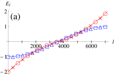
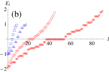
Figure 11: (Color online) (a) Spectra for $H^{(L)}$ (blue squares, $N_{L}=7141$), $H_{1}^{(C)}$ (continuous red line with crosses, $N_{C}=120$), $H_{2}^{(C)}$ (red circles, $N_{C}=80$), $H_{3}^{(C)}$ (blue triangles, $N_{C}=3571$). The cosine dispersion law of Eq.(9) is plotted as continuous blue line. Only a subset of the ordered set of all eigenvalues $E_{l}$ is plotted as function of $l$ in order to show the dispersion relation. (b) Spectra for $H^{(L)}$, $H_{1}^{(C)}$, $H_{2}^{(C)}$ and $H_{3}^{(C)}$ for $N_{L}=N_{C}=10$. Same symbols as in (a).

V Conclusion

In this article, we have shown how the way of closing a linear chain into a circular chain can lead to significantly different dynamical behavior. A single additional coupling may open access to additional parts of Hilbert space which may differ in their dimensions (and even the scaling of the dimensions with the number of spins), the physical properties of the basis functions, or give rise to different, nonequivalent matrix representations of the hamiltonian. This can modify the time-dependent polarizations on a macroscopical level, even though the hamiltonians only differ locally by one spin and its coupling to the rest of the chain. For example, the rates of change of polarization in the linear regime for $H_{3}^{(C)}$ and $H^{(L)}$ (see Eqs.(64) and (20)) differ by about $25\%$, even for arbitrarily long chains. In this case, the number of basis states of $H_{3}^{(C)}$ is twice as large as the number of basis states of $H^{(L)}$ but remains of the same order ${\cal O}(N_{L})$. When adjusted to the same dimension of the basis by changing the length of the chain, almost the same representation of the hamiltonian results, but the physical properties of the basis functions differ strongly. The rates of polarization change for $H_{1}^{(C)}$ and $H_{2}^{(C)}$ differ even from the one of $H^{(L)}$, by roughly a factor $2$ and $1.28$, respectively. Here, the number of basis states connected by $H_{1}^{(C)}$ or $H_{2}^{(C)}$ scales as ${\cal O}(N_{C}^{2})$. The matrix representations of the hamiltonians have a substantially different structure, and also the physical properties of the basis states differ. It remains to be seen whether applications can be found which exploit the high sensitivity of the time dependent polarizations to the additional local couplings used to change the boundary conditions.