Spectral radius, index estimates
for Schrödinger operators
and geometric applications

Abstract

In this paper we study the existence of a first zero and the oscillatory behavior of solutions of the ordinary differential equation $(vz^{\prime})^{\prime}+Avz=0$, where $A,v$ are functions arising from geometry. In particular, we introduce a new technique to estimate the distance between two consecutive zeros. These results are applied in the setting of complete Riemannian manifolds: in particular, we prove index bounds for certain Schrödinger operators, and an estimate of the growth of the spectral radius of the Laplacian outside compact sets when the volume growth is faster than exponential. Applications to the geometry of complete minimal hypersurfaces of Euclidean space, to minimal surfaces and to the Yamabe problem are discussed.

1 Introduction

Radialization techniques are a powerful tool in investigating complete Riemannian manifolds. In favourable circumstances these lead to the study of an ordinary differential equation in order to control the solutions of a given partial differential equation. In this respect, one of the challenging problems involved is the study of the sign of the solutions of the ODE, and the positioning of the possible zeros. In this paper we determine some conditions ensuring the oscillatory behavior, the existence of zeros and their positioning, of a solution $z(t)$ of the following Cauchy problem:

$$\left\{\begin{array}[]{l}(v(t)z^{\prime}(t))^{\prime}+A(t)v(t)z(t)=0\qquad\mathrm{on\ }(0,+\infty)\\[2.84544pt] z^{\prime}(t)=O(1)\quad\mathrm{as\ }t\downarrow 0^{+}\quad,\quad z(0^{+})=z_{0}>0\end{array}\right.$$ (1.1)

where $v(t),A(t)$ are nonnegative functions. The application of these results to the geometric problems we shall consider below leads us to assume the following structural conditions:

$$\begin{array}[]{l}\displaystyle A(t)\in L^{\infty}_{\mathrm{loc}}([0,+\infty))\quad,\quad A(t)\geq 0\quad,\quad A(t)\not\equiv 0\\[5.69046pt] \displaystyle 0\leq v(t)\in L^{\infty}_{\mathrm{loc}}([0,+\infty))\quad,\quad 1/v(t)\in L^{\infty}_{\mathrm{loc}}((0,+\infty))\\[5.69046pt] \displaystyle v(t)\text{ is non decreasing near }0\text{ and }\lim_{t\rightarrow 0^{+}}v(t)=0.\end{array}$$

Of course, requests $A,v\geq 0$, $A\not\equiv 0$ are intended in $L^{\infty}_{\mathrm{loc}}$ sense, while the last request means that there exists a version of $v(t)$ which is non-decreasing in a neighborhood of zero and whose limit as $t\rightarrow 0^{+}$ is equal to zero.
Due to the weak regularity of $v$ and $A$, solutions $z(t)$ of (1.1) are not expected to be classical, and the Cauchy problem is expected to hold almost everywhere (a.e.) on $(0,+\infty)$. Equivalently (integrating and using the condition in zero), we are interested in solutions $z(t)$ of the integral equation

$$z(t)=z_{0}-\int_{0}^{t}\frac{1}{v(s)}\left\{\int_{0}^{s}A(x)v(x)z(x)dx\right\}ds.$$

For our purposes we shall look for $z(t)\in\mathrm{Lip}_{\mathrm{loc}}([0,+\infty))$, that is, locally Lipschitz solutions. Note that the locally Lipschitz condition near zero ensures that $z^{\prime}(t)=O(1)$ hold almost everywhere in a neighborhood of zero. The existence of such solutions in our assumptions will be given in Appendix, where we will also prove that the zeros of $z(t)$, if any, are attained at isolated points.
The Cauchy problem (1.1) is a somewhat ”integrated” version of that presented in [BR], in the sense that, as we shall see, in the geometric applications the role of $v(t)$ will be played by the volume growth of geodesic spheres of some complete Riemannian manifold $M$, and $A(t)$ will represent the spherical mean of some given function $a(x)$. However, the techniques introduced here are completely different from those in [BR], and remind some in the work of Do Carmo and Zhou [DoCZ].

Nevertheless, as in [BR], we recognize an explicit critical function $\chi(t)$, depending only on $v(t)$, which serves as a border line for the behavior of $z(t)$: roughly speaking, if $A(t)$ is much greater than $\chi(t)$ in some region, then $z(t)$ has a first zero, while if $A(t)$ is not greater than $\chi(t)$ there are examples of positive solutions. We will see that $\chi(t)$ generalizes the critical functions presented in [BR].

Using $\chi(t)$ we will provide a condition in finite form for the existence and localization of a first zero of $z(t)$ (Corollary 2.3), and a sharp condition for the oscillatory behavior (Corollary 2.4). In particular, this latter Corollary improves on the application of the Hille-Nehari oscillation theorem (see [RRS]) to (1.1).

The key technical result of the paper is Theorem 4.1 which, under very general assumptions, estimates the distance between two consecutive zeros of an oscillatory solution of (1.1): denoting with $T_{1}(\tau)<T_{2}(\tau)$ the first two consecutive zeros of $z(t)$ after $t=\tau$, Theorem 4.1 states that

$$T_{2}(\tau)-T_{1}(\tau)=O(\tau)\qquad\mathrm{as\ }\tau\rightarrow+\infty.$$

This result is achieved using a new but elementary technique which highly improves on the application of Sturm’s type arguments to (1.1). Roughly speaking, the estimate will be obtained performing a careful control on the level sets of the solution of the Riccati equation associated to (1.1). Moreover, in case

$$v(t)\leq f(t)=\Lambda\exp\{at^{\alpha}\log^{\beta}t\}\qquad\Lambda,a,\alpha>0,\ \beta\geq 0,$$

we provide an upper estimate for

$$\limsup_{\tau\rightarrow+\infty}\frac{T_{2}(\tau)}{\tau}$$

with an explicit constant depending only on $\alpha$ and the growth of $A(t)$ with respect to $\chi(t)$ (more precisely, with respect to a critical curve $\chi_{f}(t)$ modelled on $f(t)$ instead of $v(t)$).

There are several geometric applications of the above results; the main idea is that (1.1) naturally appears in spectral estimates. We will follow two slightly different ways. On the one hand, we will provide an index estimate for Schrödinger type operators $L=\Delta+a(x)$, while, on the other hand, we will bound from above the growth of the spectral radius of the Laplacian outside geodesic balls, even when the volume growth of the manifold is faster than exponential. Applications naturally arise in the setting of minimal hypersurfaces of Euclidean space, their Gauss map, minimal surfaces and the Yamabe problem. We state these geometric results in the next subsections.

1.1 The geometric setting

From now on, we let $(M,\langle,\rangle)$ denote a connected, geodesically complete, non compact Riemannian manifold of dimension $m\geq 2$. Fix an origin $o\in M$ and let $r(x)=\mathrm{dist}(x,o)$ be the distance function from $o$. It is well known that $r(x)$ is a Lipschitz function on $M$ which is smooth outside $o$ and its cut-locus $\mathrm{cut}(o)$. For later use we briefly recall some basic facts on the cut-locus in case $M$ is geodesically complete; the interested reader can consult, for instance, [DoC] pp. 267-275.
Denote with $\exp$ the exponential map

$$\exp\ :\ T_{o}M\rightarrow M,$$

which, by the Hopf-Rinow theorem, is surjective and defined on the whole $T_{o}M$. The origin $o$ is called a pole of $M$ if it has no conjugate points; for example, this is the case if the sectional curvature of $M$ is non positive. It turns out that, if $o$ is a pole, $\exp$ is a covering map, hence a diffeomorphism if $M$ is simply connected. For every $w\in T_{o}M$ such that $|w|=1$, we indicate with $\gamma_{w}:[0,+\infty)\rightarrow M$ the geodesic ray starting from $o$ with velocity $1$ in the direction of $w$, and we consider

$$t_{w}=\sup\left\{s\in[0,+\infty)\ \text{ such that }\ r(\gamma_{w}(s))=s\right\}.$$

Clearly, $t_{w}>0$ because of the existence of geodesic neighborhoods. If $t_{w}<+\infty$, we define the cut-point of $o$ along $\gamma_{w}$ as $\gamma_{w}(t_{w})$. The cut-locus of $o$ is defined as the union of the cut-points of $o$ along every geodesic ray. In other words, $\mathrm{cut}(o)=\exp(\Sigma)$, where

$$\Sigma=\left\{tw\in T_{o}M\ :\ |w|=1\ \text{ and }\ t=t_{w}<+\infty\right\}.$$

It is easy to see that, if $r(\gamma_{w}(s))=s$ for some $s>0$, then the same equality holds for every $t\in[0,s)$. Therefore, if $t_{w}<+\infty$ then $\gamma_{w}$ is length minimizing for every $t\in(0,t_{w}]$ and it does not minimize length for any $t\in(t_{w},+\infty)$. By the Hopf-Rinow theorem we argue that the exponential map restricted to the set $\mathcal{U}\cup\Sigma$, where

$$\mathcal{U}=\left\{tw\in T_{o}M\ :\ |w|=1\ \text{ and }\ t<t_{w}\right\}$$

is still surjective, hence $\exp(\mathcal{U})=M\backslash\mathrm{cut}(o)=\mathrm{cut}(o)^{c}$. One can prove that

• $\mathrm{cut}(o)$ is a zero measure, closed subset of $M$, hence $\mathcal{U}=\exp^{-1}\big{\{}\mathrm{cut}(o)^{c}\big{\}}$ is open in $T_{o}M$;

• $M$ is compact if and only if, for every $w\in T_{o}M$, $t_{w}<+\infty$.

• $p\in\mathrm{cut}(o)$ if and only if either it is a conjugate point of $o$, or there exist at least 2 distinct geodesics joining $o$ to $p$ with the same length. The two possibilities do not reciprocally exclude.

• For every $q\in\exp(\mathcal{U})$, there exists a unique minimizing geodesic from $o$ to $q$. In other words, $\exp:\mathcal{U}\rightarrow\mathrm{cut}(o)^{c}$ is a bijection (indeed, a diffeomorphism).

We indicate with $B_{r}$ the geodesic ball of radius $r$ centered at $o$, with $\partial B_{r}$ its boundary and we call $\partial B_{r}\cap\mathrm{cut}(o)^{c}$ the regular part of $\partial B_{r}$. The regular part of $\partial B_{r}$ is an open set in the induced topology on $\partial B_{r}$, and $\partial B_{r}\cap\mathrm{cut}(o)^{c}$ is diffeomorphic, through the exponential map, to the set $\mathcal{U}\cap\mathbb{S}^{m-1}(r)$, where $\mathbb{S}^{m-1}(r)$ is the hypersphere

$$\mathbb{S}^{m-1}(r)=\left\{w\in T_{o}M\ :\ |w|=r\right\}.$$

We denote with $\mathrm{Vol}(\partial B_{r})$ the $(m-1)$-dimensional volume of $\partial B_{r}$, that is, the Hausdorff measure of $\partial B_{r}$. It turns out that it coincides with the induced Riemannian measure when restricted to the regular part of $\partial B_{r}$. The points of $\partial B_{r}\cap\mathrm{cut}(o)$ may be image of many points of $\Sigma\cap\mathbb{S}^{m-1}(r)$. For this reason, indicating with $\theta$ a point of the unit sphere $\mathbb{S}^{m-1}=\mathbb{S}^{m-1}(1)\subset T_{o}M$, we define the multiplicity function

$$n_{r}(\theta)=\text{ cardinality of }\{\varphi\in\mathbb{S}^{m-1}\ :\ \exp(r\theta)=\exp(r\varphi)\}\leq+\infty.$$

This coincides with the number of distinct minimizing geodesic segments joining $o$ to $q=\exp(r\theta)$, which, analogously, we denote with $n_{r}(q)$. According to the work of Grimaldi and Pansu [GP], if we set

$$\chi_{r}(\theta)=\left\{\begin{array}[]{ll}1&\text{if }\ r<t_{\theta}\\[2.84544pt] 1/n_{r}(\theta)&\text{if }\ r=t_{\theta}\\[2.84544pt] 0&\text{if }\ r>t_{\theta}\end{array}\right.\qquad\text{and}\qquad\chi_{r^{\pm}}(\theta)=\lim_{t\rightarrow r^{\pm}}\chi_{t}(\theta)$$

then the Hausdorff measure of $\partial B_{r}$ is given by

$$\mathrm{Vol}(\partial B_{r})=\int_{\mathbb{S}^{m-1}}\Theta(r,\theta)\chi_{r}(\theta)d\theta,$$

where $\Theta(r,\theta)$ is the density of the Riemannian measure. Moreover, by the dominated convergence theorem,

$$\lim_{t\rightarrow r^{\pm}}\mathrm{Vol}(\partial B_{t})=\int_{\mathbb{S}^{m-1}}\Theta(r,\theta)\chi_{r^{\pm}}(\theta)d\theta.$$

Therefore, in general circumstances $\mathrm{Vol}(\partial B_{r})$ may present discontinuities of the “first kind”, that is, at a point $r>0$ we always have the existence of finite limits both from the right and from the left, possibly with two different values. Indeed, setting $v(r)=\mathrm{Vol}(\partial B_{r})$, it is shown in [GP] that for every complete Riemannian manifold

$$v(r^{+})-v(r^{-})=-2\mathrm{Vol}(\partial B_{r}\cap\mathrm{cut}(o)).$$

The key ingredient of their proof is a technical Lemma which shows that, up to a set of $(m-1)$-dimensional measure zero, $\partial B_{r}\cap\mathrm{cut}(o)$ is made up of points having exactly $2$ distinct geodesics which minimize distance from $o$. Observe that $v(t)$ jumps downward and that, a priori, the discontinuities of $v(t)$ may be non isolated. Note also that, from the definition of $\chi_{r}(\theta)$, we get

$$\chi_{r^{+}}(\theta)=\left\{\begin{array}[]{ll}1&\text{if }\ r<t_{\theta}\\[2.84544pt] 0&\text{if }\ r=t_{\theta}\\[2.84544pt] 0&\text{if }\ r>t_{\theta}\end{array}\right.\qquad\chi_{r^{-}}(\theta)=\left\{\begin{array}[]{ll}1&\text{if }\ r<t_{\theta}\\[2.84544pt] 1&\text{if }\ r=t_{\theta}\\[2.84544pt] 0&\text{if }\ r>t_{\theta}\end{array}\right.,$$

hence from $\chi_{r^{+}}\leq\chi_{r}\leq\chi_{r^{-}}$ we deduce that $v(t)\in[v^{+}(t),v^{-}(t)]$. Therefore, a necessary and sufficient condition on $\mathrm{Vol}(\partial B_{r})$ to be continuous on $[0,+\infty)$ is given by the “transversality condition”

$$\mathrm{Vol}(\partial B_{r}\cap\mathrm{cut}(o))=0\qquad\forall\ r\geq 0.$$

However, this reasonable request sometimes is not easy to verify. This is the case, for example, when one constructs manifolds as immersed submanifolds of some ambient space. This suggests to work with discontinuous volume functions $\mathrm{Vol}(\partial B_{r})$ which will take the role of $v$ in (1.1). The next result will reveal important in what follows.

Proposition 1.2.

Let $v(r)=\mathrm{Vol}(\partial B_{r})$ be the volume of geodesic spheres of a connected, complete, non compact Riemannian manifold. Then $v(r)$ is continuous and increasing in a neighborhood of $r=0$. Furthermore,

$$v(r)=\frac{v(r^{+})+v(r^{-})}{2}\quad,\quad v(r)>0\ \text{ for }\ r>0\quad,\quad\frac{1}{v(r)}\in L^{\infty}_{\mathrm{loc}}((0,+\infty))$$ (1.2)

Proof. The first part is immediate using polar coordinates around zero. As for the first property in (1.2), we denote with $\mathcal{V}=\{w\in\mathbb{S}^{m-1}\ :\ rw\in\mathcal{U}\}$ and with $\mathcal{W}=\{w\in\mathbb{S}^{m-1}\ :\ rw\in\Sigma\}$. Since $r\mathcal{V}=\mathbb{S}^{m-1}(r)\cap\mathcal{U}$ is open, then $\mathcal{V}$ is an open set of $\mathbb{S}^{m-1}$. In polar coordinates

$$\begin{array}[]{ll}v(r)&=\displaystyle\int_{\mathbb{S}^{m-1}}\Theta(r,\theta)\chi_{r}(\theta)d\theta\equiv\int_{\mathcal{V}}\Theta(r,\theta)d\theta+\int_{\mathcal{W}}\Theta(r,\theta)\frac{1}{n_{r}(\theta)}d\theta\\[14.22636pt] &=\mathrm{Vol}(\partial B_{r}\cap\mathrm{cut}(o)^{c})+\mathrm{Vol}(\partial B_{r}\cap\mathrm{cut}(o))\\[14.22636pt] v(r^{+})&=\displaystyle\int_{\mathbb{S}^{m-1}}\Theta(r,\theta)\chi_{r^{+}}(\theta)d\theta\equiv\int_{\mathcal{V}}\Theta(r,\theta)d\theta=\mathrm{Vol}(\partial B_{r}\cap\mathrm{cut}(o)^{c})\\[14.22636pt] v(r^{-})&=\displaystyle\int_{\mathbb{S}^{m-1}}\Theta(r,\theta)\chi_{r^{-}}(\theta)d\theta\equiv\int_{\mathcal{V}}\Theta(r,\theta)d\theta+\int_{\mathcal{W}}\Theta(r,\theta)d\theta\\[14.22636pt] &=\displaystyle\mathrm{Vol}(\partial B_{r}\cap\mathrm{cut}(o)^{c})+\int_{\partial B_{r}\cap\mathrm{cut}(o)}n_{r}(x)d\sigma(x)\end{array}$$

By the Grimaldi-Pansu lemma [GP], up to a set of $(m-1)$-dimensional measure zero, the multiplicity $n_{r}(x)$ is equal to $2$. Therefore, by the above expressions is immediate to deduce that $v(r^{+})+v(r^{-})=2v(r)$. We observe now that if we prove that $1/v\in L^{\infty}_{\mathrm{loc}}((0,+\infty))$, then $v(r)>0$ on $(0,+\infty)$. Indeed, assume $v(r_{0})=0$ for some $r_{0}\in(0,+\infty)$. Then necessarily $v(r_{0}^{+})=0$, $v(r_{0}^{-})=2v(r_{0})-v(r_{0}^{+})=0$ and $1/v$ is unbounded in a neighborhood of $r_{0}$. It remains to prove that $1/v\in L^{\infty}_{\mathrm{loc}}((0,+\infty))$, that is, $v(r)$ is bounded away from zero on every compact set $K$ disjoint from $r=0$. Assume by contradiction that there exists $\{r_{k}\}\subset K$ such that $v(r_{k})\rightarrow 0$. By compactness, there exists $\widetilde{r}\in K$ such that $r_{k}\rightarrow\widetilde{r}$. Up to passing to a subsequence we have two cases: $r_{k}\uparrow\widetilde{r}$ or $r_{k}\downarrow\widetilde{r}$. In the first case $v(\widetilde{r}^{-})=0$, in the second $v(\widetilde{r}^{+})=0$. However, since $v$ jumps downward, in both cases $v(\widetilde{r}^{+})=0$. We are going to show that

$$\partial B_{\widetilde{r}}\subseteq\mathrm{cut}(o).$$ (1.3)

Indeed, let (1.3) be false, and let $q\in\partial B_{\widetilde{r}}\cap\mathrm{cut}(o)^{c}$. Since $\exp$ is a diffeomorphism in a neighborhood of $q$, we can choose a unique $\theta_{0}\in\mathcal{V}$ such that $q=\exp(\widetilde{r}\theta_{0})$. Moreover, since $\mathcal{U}$ is open, from $\widetilde{r}\theta_{0}\in\mathcal{U}$ we can chose a neighborhood $\mathcal{J}$ with compact closure in $\mathcal{U}$ of the form

$$\mathcal{J}=\{r\theta\ :\ r\in(\widetilde{r}-2\varepsilon,\widetilde{r}+2\varepsilon)\ ,\ \theta\in\mathcal{V}_{\theta_{0}}\},$$

where $\varepsilon>0$ is sufficiently small and $\mathcal{V}_{\theta_{0}}$ is a neighborhood of $\theta_{0}$ on the unit sphere $\mathbb{S}^{m-1}$, independent from $\varepsilon$. Since the Riemannian density $\Theta$ is smooth and positive, there exists $C>0$ independent of $\varepsilon$ such that $\Theta(r,\theta)\geq C$ on $\mathcal{J}$. It follows that

$$v(\widetilde{r}+\varepsilon)=\int_{\mathbb{S}^{m-1}}\Theta(\widetilde{r}+\varepsilon,\theta)\chi_{\widetilde{r}+\varepsilon}(\theta)d\theta\geq\int_{\mathcal{V}_{\theta_{0}}}Cd\theta=C\mathrm{Vol}_{\mathrm{Eucl}}(\mathcal{V}_{\theta_{0}})\qquad\forall\ \varepsilon.$$

This contradicts $v(\widetilde{r}^{+})=0$ and proves (1.3). By (1.3) we deduce that, for every geodesic ray $\gamma_{w}$ starting from $o$, there exists $t_{w}\leq r$ such that $\gamma_{w}(t_{w})\in\mathrm{cut}(o)$. Therefore, $M$ is compact with diameter $\leq 2r$, against our assumptions. $\blacktriangle$

Let $s(x)$ be the scalar curvature of $(M,\langle,\rangle)$. The previous proposition enables us to define the spherical mean

$$S(r)=\frac{1}{\mathrm{Vol}(\partial B_{r})}\int_{\partial B_{r}}s$$

on the whole $(0,+\infty)$. $S(r)$ is continuous in a neighborhood of zero with $\lim_{r\rightarrow 0^{+}}S(r)=s(o)$, and possesses at least the same regularity as $\mathrm{Vol}(\partial B_{r})$. In case $(\mathrm{Vol}(\partial B_{r}))^{-1}\in L^{1}(+\infty)$ we define the critical function

$$\chi(r)=\Big{(}2\mathrm{Vol}(\partial B_{r})\int_{r}^{+\infty}\frac{ds}{\mathrm{Vol}(\partial B_{s})}\Big{)}^{-2}\ \ \in L^{\infty}_{\mathrm{loc}}((0,+\infty)),$$ (1.4)

that we shall consider below.

Since in the sequel we will be concerned with spectral arguments, we briefly recall some definitions. Let $\Delta$ denote the Laplace-Beltrami operator on $M$, and consider a differential operator $L=\Delta+a(x)$, where $a(x)\in C^{0}(M)$, and a bounded domain $\Omega\subset M$. The $k$-th eigenvalue $\lambda_{k}^{L}(\Omega)$, of $L$ on $\Omega$ (counted with its multiplicity) is defined by Rayleigh characterization:

$$\lambda_{k}^{L}(\Omega)=\inf_{\scriptsize{\begin{array}[]{c}V_{k}\leq C^{\infty}_{0}(\Omega)\\[2.84544pt] \dim(V_{k})=k\end{array}}}\left(\sup_{0\neq\phi\in V_{k}}\frac{\int_{\Omega}{|\nabla\phi|^{2}}-\int_{\Omega}a\phi^{2}}{\int_{\Omega}\phi^{2}}\right),$$ (1.5)

where we can substitute $C^{\infty}_{0}(\Omega)$ with $\mathrm{Lip}_{0}(\Omega)$. If $\Omega$ has sufficiently regular boundary, $\lambda_{1}^{L}(\Omega)$ is achieved by the non zero solutions of the Dirichlet problem

$$\left\{\begin{array}[]{l}Lu+\lambda_{1}^{L}(\Omega)u=0\qquad{\rm on}\ \Omega\\ u\equiv 0\qquad{\rm on}\ \partial\Omega\end{array}\right.$$ (1.6)

Note that $L$ is non positive on $C^{\infty}_{0}(\Omega)$ if and only if $\lambda_{1}^{L}(\Omega)\geq 0$. The main example of a non positive operator on every $\Omega$ is the Laplacian itself.

We define the index $\mathrm{ind}_{L}(\Omega)$ as the number of negative eigenvalues of $-L$. By Rellich Theorem, this number is finite. Indeed, using Rayleigh characterization

$$\lambda_{k}^{L}(\Omega)\geq\lambda_{k}^{\Delta}(\Omega)-\|a\|_{L^{\infty}(\Omega)},$$

therefore $\widetilde{L}=L-\|a\|_{L^{\infty}(\Omega)}$ is strictly non positive on $C^{\infty}_{0}(\Omega)$, hence it is invertible. The Friedrich extension of $(-\widetilde{L})^{-1}:L^{2}(\Omega)\rightarrow L^{2}(\Omega)$ is a compact operator, so that its spectrum consists in a discrete sequence $\{\lambda_{j}\}$ of eigenvalues, each of them with finite multiplicity. It follows that the spectrum of $-L$ is $\{\lambda_{j}-\|a\|_{L^{\infty}(\Omega)}\}$, and $\mathrm{ind}_{L}(\Omega)$ is clearly finite. The bottom of the spectrum of $L$ on $M$, also called the first eigenvalue or the spectral radius, $\lambda_{1}^{L}(M)$, is defined by

$$\lambda_{1}^{L}(M)=\inf\left\{\lambda_{1}^{L}(\Omega)\ :\ \Omega\subset M\ {\rm is}\ {\rm a}\ {\rm bounded}\ {\rm domain}\right\}$$ (1.7)

Let $Z\subset M$ be a subset. We define the first eigenvalue of $L$ on the ”punctured” manifold $M\backslash Z$ by

$$\lambda_{1}^{L}(M\backslash Z)=\inf\left\{\lambda_{1}^{L}(\Omega)\ :\ \Omega\subset M\backslash Z\ {\rm is}\ {\rm a}\ {\rm bounded}\ {\rm domain}\right\}$$ (1.8)

Similarly, the index of $L$ on $M$ is defined by

$$\mathrm{ind}_{L}(M)=\sup\left\{\mathrm{ind}_{L}(\Omega)\ :\ \Omega\subset M\ {\rm is}\ {\rm a}\ {\rm bounded}\ {\rm domain}\right\}$$

and it may be infinite. Note that $\mathrm{ind}_{L}(M)=0$ if and only if $\lambda_{1}^{L}(M)\geq 0$.

1.3 Spectral estimates: the two main results

The first theorem deals with the index of $L$.

Theorem 1.4.

Let $a(x)\in C^{0}(M)$. Suppose that the spherical mean $A(r)$ of $a(x)$ is non negative and not identically null. Consider the following assumptions:

• either

  $$(\mathrm{Vol}(\partial B_{r}))^{-1}\not\in L^{1}(+\infty)$$

  or $(\mathrm{Vol}(\partial B_{r}))^{-1}\in L^{1}(+\infty)$ and there exist $0<R_{0}<R_{1}$ such that $A(r)\not\equiv 0$ on $[0,R_{0}]$ and

  $$\int^{R_{1}}_{R_{0}}\big{(}\sqrt{A(s)}-\sqrt{\chi(s)}\big{)}ds>-\frac{1}{2}\Big{(}\log\int_{B_{R_{0}}}a+\log\int_{R_{0}}^{+\infty}{\frac{ds}{\mathrm{Vol}(\partial B_{s})}}\Big{)}$$ (1.9)

• either

  $$(\mathrm{Vol}(\partial B_{r}))^{-1}\not\in L^{1}(+\infty)\quad,\quad a(x)\not\in L^{1}(M)$$ (1.10)

  or

  $$(\mathrm{Vol}(\partial B_{r}))^{-1}\in L^{1}(+\infty)\quad,\quad\limsup_{r\rightarrow+\infty}\int_{R}^{r}\big{(}\sqrt{A(s)}-\sqrt{\chi(s)}\big{)}ds=+\infty.$$ (1.11)

  for some $R$ sufficiently large.

• $(\mathrm{Vol}(\partial B_{r}))^{-1}\in L^{1}(+\infty)$,

  $$\mathrm{Vol}(\partial B_{r})\leq\Lambda\exp\{ar^{\alpha}\log^{\beta}r\}\qquad\mathit{for\ some\ }\Lambda,a,\alpha>0,\ \beta\geq 0$$

  and, for some $R>0$, $c>1$,

  $$\sqrt{A(r)}\geq c\Big{(}\frac{a\alpha}{2}\Big{)}r^{\alpha-1}\log^{\beta}r\qquad\forall\ r\geq R$$ (1.12)

Let $L=\Delta+a(x)$. Then

• under assumption $(i)$, $\lambda_{1}^{L}(M)<0$;

• under assumption $(ii)$, $L$ is unstable at infinity, that is, $\lambda_{1}^{L}(M\backslash B_{R})<0$ for every $R>0$. In particular, $L$ has infinite index;

• under assumption $(iii)$, $L$ is unstable at infinity and

  $$\liminf_{r\rightarrow+\infty}\frac{\mathrm{ind}_{L}(B_{r})}{\log r}\geq\frac{\alpha}{2\log\Big{(}\frac{c+1}{c-1}\Big{)}}.$$ (1.13)

We observe that (1.11) and (1.12) are conditions “at infinity” and they are typical of oscillation results. On the other hand, condition (1.9) deserves some special attention since it is in finite form, in the sense that it only involves the behavior of $a(x)$ on a compact set, namely $B_{R_{1}}$: the left hand side states how much must $a(x)$ exceed the critical curve on the compact annular region $\overline{B}_{R_{1}}\backslash B_{R_{0}}$ in order to have a negative spectral radius, and it only depends on the behavior of $a(x)$ near zero (on $B_{R_{0}}$) and on the geometry at infinity of $M$. Note also that $R_{1}$ does not appear in the right hand side of (1.9).

Remark 1.5.

By a famous result of Fisher-Colbrie [FC], condition $\mathrm{Ind}_{L}(M)<\infty$ implies the stability at infinity (that is, $\lambda_{1}^{L}(M\backslash B_{R})\geq 0$ for some $R\geq 0$). As far as we know, it is yet an open problem to prove the converse, or to provide an explicit counterexample. However, we remark that a sufficient condition to have finite index is that the strict inequality $\lambda_{1}^{L}(M\backslash B_{R})>0$ hold for some $R$. For a detailed account of spectral theory for Schrödinger operators on Riemannian manifolds we refer the reader to [PRS1].

The second result can be probably regarded as the core of the paper: it provides a sharp upper bound for the growth of $\lambda_{1}^{\Delta}(M\backslash B_{R})$ as a (monotone) function of $R$. In the literature, bounds for the spectral radius on $M$ are obtained under at most exponential volume growth of geodesic spheres. On the contrary, Theorem 1.6 works also with faster volume growths. To better appreciate the result that we shall introduce below, we begin with some preliminary considerations.

It is well known that, if $Z$ is any compact subset of $\mathbb{R}^{m}$, then $\lambda_{1}^{\Delta}(\mathbb{R}^{m}\backslash Z)=0$. Extending a result of Cheng and Yau [CY], Brooks [B] has shown that if the manifold $(M,\langle,\rangle)$ has at most sub-exponential volume growth then $\lambda_{1}^{\Delta}(M)=0$. However, if we puncture the manifold by a compact set $Z\not=\emptyset$, contrary to the case of $\mathbb{R}^{m}$, it may happen that $\lambda_{1}^{\Delta}(M\backslash Z)\not=0$. Indeed, Do Carmo and Zhou, [DoCZ], give an example where $\mathrm{Vol}(M)<+\infty$ and

$$\lambda_{1}^{\Delta}(M\backslash\overline{B}_{1})\geq\frac{1}{4}$$

Moreover, up to the missing requirement of continuity of $\mathrm{Vol}(\partial B_{r})$, they prove that in case $M$ has infinite volume,

• if $M$ has sub-exponential volume growth of geodesic spheres, then

  $$\lambda_{1}^{\Delta}(M\backslash B_{R})=0\qquad\forall\ R\geq 0;$$ (1.14)

• if $\mathrm{Vol}(\partial B_{r})\leq C{\rm e}^{ar}$ for some $C,a>0$, then

  $$\lambda_{1}^{\Delta}(M\backslash B_{R})\leq\frac{a^{2}}{4}\qquad\forall\ R\geq 0.$$ (1.15)

It is interesting to see what happens when the volume growth is faster than exponential. Towards this aim, we extend Do Carmo and Zhou’s example to grasp the situation a step further. Thus we consider the model, in the sense of Greene and Wu, $(M,ds^{2})=(\mathbb{R}^{m},ds^{2})$, with metric given in polar coordinates by

$$ds^{2}=dr^{2}+h(r)^{2}d\theta^{2}$$ (1.16)

where $h\in C^{\infty}([0,+\infty))$ is positive on $(0,+\infty)$ and satisfies

$$h(r)=\left\{\begin{array}[]{l}\displaystyle r\quad{\rm on}\ [0,1]\\[5.69046pt] \displaystyle\exp\left\{\frac{ar^{\alpha}}{m-1}\right\}\quad{\rm on}\ [2,+\infty)\end{array}\right.$$ (1.17)

for some $a>0,\ \alpha\geq 1$. Note that (1.16) extends smoothly at the origin because of the definition of $h$ near 0, and that, for $r\geq 2$, $\mathrm{Vol}(\partial B_{r})=\exp\{ar^{\alpha}\}$. We let $b\in(0,a)$ and set

$$u_{b}(x)={\rm e}^{-br(x)^{\alpha}}\qquad{\rm on}\ M\backslash B_{2}.$$ (1.18)

A simple checking shows that

$$\Delta u_{b}+\lambda_{b}(r)u_{b}=0\qquad{\rm on}\ M\backslash B_{2},$$

where $\lambda_{b}(r)$ is defined as

$$\lambda_{b}(r)=\alpha^{2}b(a-b)r^{2(\alpha-1)}+\alpha(\alpha-1)br^{\alpha-2}.$$ (1.19)

Observe that, in case $\alpha=1$, $\lambda_{b}(r)\equiv b(a-b)$, while, if $\alpha>1$, $\lambda_{b}(r)$ is strictly increasing on $(R_{0},+\infty)$, with $R_{0}$ sufficiently large that

$$2\alpha(a-b)R_{0}^{\alpha}+(\alpha-2)>0.$$

Up to further enlarging $R_{0}$, we can also assume that

$$\frac{\alpha-1}{2\alpha}\frac{1}{r^{\alpha}}<\frac{a}{2}\qquad{\rm for}\ r\geq R_{0}.$$ (1.20)

Applying a result of Cheng and Yau, [CY] we have that, for every $b\in(0,a)$, $R\geq R_{0}$,

$$\lambda_{1}^{\Delta}(M\backslash B_{R})\geq\inf_{M\backslash B_{R}}{-\frac{\Delta u_{b}}{u_{b}}}=\inf_{[R,+\infty)}{\lambda_{b}(r)}=\lambda_{b}(R)$$

The choice

$$\widetilde{b}=\frac{a}{2}+\frac{\alpha-1}{2\alpha}\frac{1}{R^{\alpha}}$$

maximize $\lambda_{b}(R)$ and $\widetilde{b}\in(0,a)$ because of (1.20). Then, for $R\geq R_{0}$

$$\lambda_{1}^{\Delta}(M\backslash B_{R})\geq\alpha^{2}\left(\frac{a^{2}}{4}-\frac{(\alpha-1)^{2}}{4\alpha^{2}}\frac{1}{R^{2\alpha}}\right)R^{2(\alpha-1)}$$ (1.21)

Note that for $\alpha=1$ the above reduces to

$$\lambda_{1}^{\Delta}(M\backslash B_{R})\geq\frac{a^{2}}{4}$$

In particular, this shows that the upper bound in Theorem 3.1 in [DoCZ] is sharp. This example, for $\mathrm{Vol}(\partial B_{r})\leq C{\rm e}^{ar^{\alpha}}$, $C,a>0$, $\alpha\geq 1$, suggests to look for an upper bound of $\lambda_{1}^{\Delta}(M\backslash B_{R})$ of the form

$$C_{1}R^{2(\alpha-1)}$$

with $C_{1}=C_{1}(a,\alpha)>0$. The guess is indeed correct, as Theorem 1.6 shows.

Theorem 1.6.

If $M$ is a connected, complete, non compact Riemannian manifold such that

$$(\mathrm{Vol}(\partial B_{r}))^{-1}\in L^{1}(+\infty)\quad,\quad\mathrm{Vol}(\partial B_{r})\leq\Lambda\exp[ar^{\alpha}\log^{\beta}r]\qquad{\rm for}\ r\ {\rm large,}$$

for some $\Lambda,a,\alpha>0,\ \beta\geq 0$, the following estimates hold:

• If $0<\alpha<1$ then

  $$\lambda_{1}^{\Delta}(M\backslash B_{R})=0\qquad\forall\ R\geq 0.$$

• If $\alpha\geq 1$ then

  $$\limsup_{R\to+\infty}\Bigg{(}\frac{\lambda_{1}^{\Delta}(M\backslash B_{R})}{R^{2(\alpha-1)}\log^{2\beta}R}\Bigg{)}\leq\frac{a^{2}\alpha^{2}}{4}\inf_{c\in(1,+\infty)}\Big{\{}c^{2}\Big{(}\frac{c+1}{c-1}\Big{)}^{\frac{4(\alpha-1)}{\alpha}}\Big{\}}$$ (1.22)

Remark 1.7.

Note that $(\mathrm{Vol}(\partial B_{r}))^{-1}\in L^{1}(+\infty)$ implies $\mathrm{Vol}(M)=\infty$. This follows from Schwarz inequality

$$\int_{r}^{R}\frac{ds}{\mathrm{Vol}(\partial B_{s})}\int_{r}^{R}\mathrm{Vol}(\partial B_{s})ds\geq(R-r)^{2}$$

letting $R\rightarrow+\infty$.

We stress that the hypothesis $\mathrm{Vol}(M)=\infty$ is essential. In fact, Do Carmo and Zhou example quoted above shows that the theorem fails if $\mathrm{Vol}(M)<\infty$. On the contrary, the stronger assumption $(\mathrm{Vol}(\partial B_{r}))^{-1}\in L^{1}(+\infty)$ is for convenience: if it fails, we will show in Lemma 5.13 that $\lambda_{1}^{\Delta}(M\backslash B_{R})=0$ for every $R\geq 0$. We underline that in Theorem 1.6 we have been considering volume growth assumptions, which are weaker and more general than the usual curvature conditions used in estimating $\lambda_{1}^{\Delta}(M)$ (see for instance [P]). It is also worth mentioning that the problem of estimating $\lambda_{1}^{\Delta}(M\backslash B_{R})$ from above arises naturally in the study of unstable hypersurfaces with constant mean curvature: see for example [DoCZ] for details and further references.

1.8 Geometric consequences

The first geometric consequence is the following density theorem for complete minimally immersed hypersurfaces of Euclidean space.

Theorem 1.9.

Let $\varphi:M\rightarrow\mathbb{R}^{m+1}$ be a minimal hypersurface. We identify $T_{x}M$ with $\varphi_{\ast}T_{x}M$ viewed as an affine hyperplane in $\mathbb{R}^{m+1}$ passing through $\varphi(x)$. Assume that

$$(\mathrm{Vol}(\partial B_{r}))^{-1}\not\in L^{1}(+\infty)\quad,\quad s(x)\not\in L^{1}(M)$$ (1.23)

or that

$$(\mathrm{Vol}(\partial B_{r}))^{-1}\in L^{1}(+\infty)\quad,\quad\mathrm{Vol}(\partial B_{r})\leq\Lambda\exp\{r^{\alpha}\}\\$$ (1.24)

$$S(r)\leq-\frac{C}{r^{\mu}}$$ (1.25)

for $r\gg 1$ and some constants $C,\Lambda,\alpha>0$, $\mu\in\mathbb{R}$, with

$$2\alpha<2-\mu.$$ (1.26)

Then, for every compact set $\Omega\subseteq M$

$$\bigcup_{x\in M\backslash\Omega}T_{x}M\equiv\mathbb{R}^{m+1}$$ (1.27)

We note that Halpern [H] has proved that, when the hypersurface is compact and orientable, $\bigcup_{x\in M}T_{x}M\not\equiv\mathbb{R}^{m+1}$ if and only if $M$ is embedded as the boundary of an open star-shaped domain of $\mathbb{R}^{m+1}$. In case $M$ is non compact there are many examples with $\bigcup_{x\in M}T_{x}M\not\equiv\mathbb{R}^{m+1}$, for instance cylinders over suitable curves. However, in case $m=2$ complete minimal surfaces in $\mathbb{R}^{3}$ for which $\bigcup_{x\in M}T_{x}M\not\equiv\mathbb{R}^{3}$ are planes: this has been proved by Hasanis and Koutroufiotis in [HK].

In an analogous way, we prove the following result.

Theorem 1.10.

Let $\varphi:M\rightarrow\mathbb{R}^{m+1}$ be a connected, complete non compact minimal hypersurface. Assume that either

$$(\mathrm{Vol}(\partial B_{r}))^{-1}\not\in L^{1}(+\infty)\quad,\quad s(x)\not\in L^{1}(M)$$ (1.28)

or that, for some $C,\Lambda,\alpha>0$, $\mu\in\mathbb{R}$

$$\begin{array}[]{l}\displaystyle(\mathrm{Vol}(\partial B_{r}))^{-1}\in L^{1}(+\infty)\quad,\quad\mathrm{Vol}(\partial B_{r})\leq\Lambda\exp\{r^{\alpha}\}\\[8.5359pt] \displaystyle S(r)\leq-\frac{C}{r^{\mu}}\qquad\text{and}\qquad 2\alpha<2-\mu.\end{array}$$ (1.29)

Fix an equator $E$ in $\mathbb{S}^{m}$. Then the spherical Gauss map $\nu$ meets $E$ infinitely many times along a divergent sequence in M.

Note that we have not assumed the orientability of $M$; hence, the spherical Gauss map is only locally defined. However, due to the central symmetry of the equators, the conclusion of the theorem does not depend on the chosen local orientation: if $\nu(x)\in E$, then also $-\nu(x)\in E$.

As a third consequence of Theorem 1.4, we have the following result of Fisher-Colbrie [FC] and Gulliver [G].

Theorem 1.11.

Let $N$ be a flat $3$-manifold, and let $\varphi:M\rightarrow N$ be a simply connected, minimally immersed surface. We denote with $K$ the (necessarily non positive) sectional curvature of $M$.
Consider the stability operator $L=\Delta+|II|^{2}$. If $M$ is stable at infinity (in particular, if $\mathrm{Ind}_{L}(M)<\infty$), then $M$ is parabolic and

$$\int_{M}|K|<+\infty.$$ (1.30)

Remark 1.12.

Indeed, it is shown in [FC] that

$$\int_{M}|K|<+\infty\Longleftrightarrow\mathrm{Ind}_{L}(M)<\infty.$$

Combining with the above result yields that if a simply connected, minimal surface in $\mathbb{R}^{3}$ is stable at infinity, then its stability index is finite. Therefore, referring to Remark 1.5, a possible counterexample to the equivalence between $\mathrm{Ind}_{L}(M)<\infty$ and $\lambda_{1}^{L}(M\backslash B_{R})\geq 0$ must not be searched in the setting of minimal surfaces in $\mathbb{R}^{3}$, when $L$ is the stability operator.

With the same technique, we recover a well known result of Do Carmo and Peng [DoCP], Fisher-Colbrie and Schoen [FCS] and Pogorelov [Po].

Corollary 1.13.

Let $\varphi:M\rightarrow\mathbb{R}^{3}$ be a minimally immersed surface. If $M$ is stable, then $M$ is totally geodesic (hence, an affine plane).

The last geometrical application employs directly Theorem 1.4, together with Theorems $2.4$ and $2.1$ of [PRS], to yield the following existence result for the Yamabe problem which requires no assumptions on the Ricci curvature.

Theorem 1.14.

Suppose that the dimension of $M$ is $m\geq 3$ and that the spherical mean $S(r)$ satisfies

$$S(r)\leq 0\quad\mathit{on\ }[0,+\infty)\quad,\quad S\not\equiv 0$$

Let $k(x)\in C^{\infty}(M)$ be non positive on $M$ and strictly negative outside a compact set. Set $\mathcal{K}_{0}=k^{-1}\{0\}$ and, for

$$L=\Delta-\frac{1}{c_{m}}s(x)\qquad\mathit{where}\quad c_{m}=\frac{4(m-1)}{m-2},$$

define $\lambda_{1}^{L}(\mathcal{K}_{0})=\sup_{D}\lambda_{1}^{L}(D)$, where $D$ varies among all open sets with smooth boundary containing $\mathcal{K}_{0}$. Suppose

$$\lambda_{1}^{L}(\mathcal{K}_{0})>0.$$

Assume that either $(\mathrm{Vol}(\partial B_{r}))^{-1}\not\in L^{1}(+\infty)$ or otherwise that there exists $0<R_{0}<R_{1}$ such that $S\not\equiv 0$ on $[0,R_{0}]$ and

$$\int^{R_{1}}_{R_{0}}\big{(}\sqrt{\frac{|S(t)|}{c_{m}}}-\sqrt{\chi(t)}\big{)}dt>-\frac{1}{2}\Big{(}\log\int_{B_{R_{0}}}\frac{|s(x)|}{c_{m}}+\log\int_{R_{0}}^{+\infty}{\frac{dt}{\mathrm{Vol}(\partial B_{t})}}\Big{)}$$ (1.31)

Then, the metric $\langle,\rangle$ can be conformally deformed to a new metric of scalar curvature $k(x)$.

As the discussion after Theorem 1.4 suggests, this latter result implies that a strongly negative scalar curvature on a compact region $\Omega$ gives the existence of the conformal deformation independently of the behavior of $s(x)$ outside $\Omega$.

2 Existence of a first zero and oscillations

Fix $R\in(0,+\infty]$ (note that the value $+\infty$ is allowed), and consider the following set of assumptions:

$$0\leq A(t)\in L^{\infty}_{\mathrm{loc}}([0,R))\quad,\quad A\not\equiv 0\quad\text{in }L^{\infty}_{\mathrm{loc}}\text{ sense}$$ (A1)

$$0\leq v(t)\in L^{\infty}_{\mathrm{loc}}([0,R))\quad,\quad\frac{1}{v(t)}\in L^{\infty}_{\mathrm{loc}}((0,R))\quad,\quad\lim_{t\rightarrow 0^{+}}v(t)=0$$ (V1)

In case $1/v\in L^{1}(R^{-})$, we define the critical function

$$\chi_{R}(t)=\Big{(}\displaystyle 2v(t)\int_{t}^{R}\frac{ds}{v(s)}\Big{)}^{-2}=\Big{[}\Big{(}-\frac{1}{2}\log\int_{t}^{R}\frac{ds}{v(s)}\Big{)}^{\prime}\Big{]}^{2}\quad\in L^{\infty}_{\mathrm{loc}}((0,R))$$ (2.1)

For the ease of notation we write $\chi(t)$ in case $R=+\infty$. We are now ready to prove:

Theorem 2.1.

Let $A,v$ satisfy (A1), (V1) and let $z\in\mathrm{Lip}_{\mathrm{loc}}([0,R))$ be a positive solution of

$$\left\{\begin{array}[]{l}(v(t)z^{\prime}(t))^{\prime}+A(t)v(t)z(t)=0\qquad\text{almost everywhere on }(0,R)\\[5.69046pt] z^{\prime}(t)=O(1)\quad\mathrm{as\ }t\downarrow 0^{+}\quad,\quad z(0^{+})=z_{0}>0\end{array}\right.$$ (2.2)

Then

$$\frac{1}{v}\in L^{1}(R^{-})$$ (2.3)

and for every $0<T<t<R$ such that $A\not\equiv 0$ in $L^{\infty}([0,T])$

$$\int_{T}^{t}\big{(}\sqrt{A(s)}-\sqrt{\chi_{R}(s)}\big{)}ds\leq-\frac{1}{2}\Big{(}\log\int_{0}^{T}A(s)v(s)ds+\log\int_{T}^{R}\frac{ds}{v(s)}\Big{)}$$ (2.4)

Proof. We set

$$y(t)=-\frac{v(t)z^{\prime}(t)}{z(t)}\qquad\text{on }(0,R)$$ (2.5)

Then $y\in\mathrm{Lip}_{\mathrm{loc}}([0,R))$; this follows since $(vz^{\prime})^{\prime}=-Avz\in L^{\infty}_{\mathrm{loc}}([0,R))$, therefore $vz^{\prime}$ is locally Lipschitz. Moreover, from (V1) and (2.2) we deduce that $y(0^{+})=0$. Differentiating, we can argue that $y(t)$ satisfies Riccati equation

$$y^{\prime}=A(t)v(t)+\frac{1}{v(t)}y^{2}\qquad\text{a.e. on }(0,R)$$ (2.6)

Note that, since $A(t)\not\equiv 0$, $z$ is non constant and $y\not\equiv 0$. Moreover, $y^{\prime}(t)\geq 0$ almost everywhere on $(0,R)$. From (A1) and (2.6) it follows that, for every $T>0$ such that $A\not\equiv 0$ on $[0,T]$

$$y(t)\geq y(T)\geq\int_{0}^{T}A(s)v(s)ds>0\qquad\forall\ t\in[T,R)$$ (2.7)

From (2.6) and the elementary inequality $\epsilon a^{2}+\epsilon^{-1}b^{2}\geq 2|a||b|$, $a,b\in\mathbb{R}$, $\epsilon>0$ we also deduce $y^{\prime}\geq 2\sqrt{A(t)}|y(t)|$ and therefore

$$y^{\prime}\geq 2\sqrt{A(t)}y\qquad\text{a.e. on }[T,R)$$ (2.8)

From (2.7) and (2.8) we infer

$$y(t)\geq\Big{(}\int_{0}^{T}A(s)v(s)ds\Big{)}{\rm e}^{2\int_{T}^{t}{\sqrt{A(s)}ds}}\qquad\text{on }[T,R)$$ (2.9)

Moreover, from (2.6) and (A1),

$$\frac{y^{\prime}}{y^{2}}\geq\frac{1}{v(t)}\qquad\text{a.e. on }[T,R)$$ (2.10)

Integrating on $[t,R-\varepsilon]$ for some small $\varepsilon>0$ we get

$$\frac{1}{y(t)}\geq\frac{1}{y(R-\varepsilon)}+\int_{t}^{R-\varepsilon}\frac{ds}{v(s)}\geq\int_{t}^{R-\varepsilon}\frac{ds}{v(s)}$$ (2.11)

Letting $\varepsilon\rightarrow 0^{+}$ we obtain (2.3), and using (2.11) into (2.9) we reach the following inequality:

$$\int^{t}_{T}{\sqrt{A(s)}ds}\leq-\frac{1}{2}\log\int_{0}^{T}A(s)v(s)ds-\frac{1}{2}\log\int_{t}^{R}{\frac{ds}{v(s)}}$$ (2.12)

Inequality (2.4) is simply a rewriting of (2.12): it is enough to point out that

$$-\frac{1}{2}\log\int_{t}^{R}{\frac{ds}{v(s)}}=-\frac{1}{2}\log\int_{T}^{R}{\frac{ds}{v(s)}}+\int_{T}^{t}\sqrt{\chi_{R}(s)}ds$$ (2.13)

which follows integrating the definition of $\chi_{R}(t)$. $\blacktriangle$

Although very simple, inequality (2.4) is deep. As we have already stressed in the Introduction, the right hand side of (2.4) is independent both of $t$ and of the behavior of $A$ after $T$: if (2.4) is contradicted for some $0<T<t<R$, the left hand side represents how much must $A(t)$ exceed the critical curve on the compact region $[T,t]$ in order to have a first zero of $z(t)$, and it only depends on the behavior of $A$ and $v$ before $T$ (the first addendum of the right hand side), and on the growth of $v$ after $T$.

For geometrical purposes, from now on we will focus on the case $R=+\infty$. However, the next corollaries can be restated on $(0,R)$ replacing $+\infty$ with $R$ and $\chi(t)$ with $\chi_{R}(t)$.

Remark 2.2.

Consider (2.13) with $R=+\infty$:

$$-\frac{1}{2}\log\int_{t}^{+\infty}{\frac{ds}{v(s)}}=-\frac{1}{2}\log\int_{T}^{+\infty}{\frac{ds}{v(s)}}+\int_{T}^{t}\sqrt{\chi(s)}ds\quad,$$

valid for $1/v\in L^{1}(+\infty)$. Letting $t\rightarrow+\infty$ we deduce that

$$\sqrt{\chi(t)}\not\in L^{1}(+\infty)$$ (2.14)

Corollary 2.3 (Existence of a first zero).

In the assumptions of Theorem 2.1 with $R=+\infty$, suppose that either $1/v\not\in L^{1}(+\infty)$ or otherwise there exist $0<T<t$ such that

$$\int^{t}_{T}\big{(}\sqrt{A(s)}-\sqrt{\chi(s)}\big{)}ds>-\frac{1}{2}\Big{(}\log\int_{0}^{T}A(s)v(s)ds+\log\int_{T}^{+\infty}{\frac{ds}{v(s)}}\Big{)}$$ (2.15)

Then, for every solution $z(t)\in\mathrm{Lip}_{\mathrm{loc}}([0,+\infty))$ of (2.2), there exists $T_{0}=T_{0}(z)>0$ such that $z(T_{0})=0$. Moreover, the first zero is attained on $(0,\overline{R}]$, where $\overline{R}>0$ is the unique real number satisfying

$$\int^{t}_{T}{\sqrt{A(s)}ds}=-\frac{1}{2}\log\int_{0}^{T}A(s)v(s)ds-\frac{1}{2}\log\int_{t}^{\overline{R}}{\frac{ds}{v(s)}}$$ (2.16)

Proof. Observe that (2.15) is equivalent to say that (2.4) with $R=+\infty$ is false for some $0<T<t$. Hence, the existence of a first zero on $(0,+\infty)$ is immediate from Theorem 2.1.

As for the position of $T_{0}$, note first that (2.4) is a rewriting of (2.12). Suppose that $1/v\in L^{1}(+\infty)$. We note that the $RHS$ of (2.12) is strictly decreasing as a function of $R\in(t,+\infty)$, $\lim_{R\rightarrow t^{-}}RHS=+\infty$, and (2.12) is contradicted for $R=+\infty$ by assumption (2.15). Therefore, there exists a unique $\overline{R}\in(t,+\infty)$ such that (2.16) holds. Choosing $\varepsilon>0$ and applying Theorem 2.1 on the interval $(0,\overline{R}+\varepsilon)$ we deduce the existence of a first zero on $(0,\overline{R}+\varepsilon)$. Letting $\varepsilon\rightarrow 0$ we reach the desired conclusion.

The case $1/v\not\in L^{1}(+\infty)$ is similar: we restrict the considerations on a finite interval $[0,R]$, with $R>t$ small enough that (2.12) holds on $[0,R]$. Then, we enlarge $R$ in such a way to reach the equality in (2.12), and we conclude as in the previous case. $\blacktriangle$

Corollary 2.4 (Oscillatory behavior).

Fix $t_{0}\in(0,+\infty)$. Suppose that (A1), (V1) are met on $[t_{0},+\infty)$, with $1/v\in L^{\infty}_{\mathrm{loc}}([t_{0},+\infty))$, and let $z_{0}\in\mathbb{R}\backslash\{0\}$. Assume that either

$$\frac{1}{v(t)}\not\in L^{1}(+\infty)\quad,\quad A(t)v(t)\not\in L^{1}(+\infty)$$ (2.17)

or

$$\frac{1}{v(t)}\in L^{1}(+\infty)\quad,\quad\limsup_{t\rightarrow+\infty}\int_{T}^{t}\big{(}\sqrt{A(s)}-\sqrt{\chi(s)}\big{)}ds=+\infty$$ (2.18)

for some (hence any) $T>t_{0}$. Then, every solution $z(t)\in\mathrm{Lip}_{\mathrm{loc}}([t_{0},+\infty))$ of

$$\left\{\begin{array}[]{l}(v(t)z^{\prime}(t))^{\prime}+A(t)v(t)z(t)=0\qquad\text{a.e. on }(t_{0},+\infty)\\[5.69046pt] z(t_{0})=z_{0}\end{array}\right.$$ (2.19)

is oscillatory.

Proof. First, we claim that the two conditions in (2.18) imply that $A(t)v(t)\not\in L^{1}(+\infty)$. Indeed, from (2.14) and the second condition of (2.18) it follows that $\sqrt{A(t)}\not\in L^{1}(+\infty)$, and from Cauchy-Schwarz inequality

$$\Big{(}\int_{T}^{t}A(s)v(s)\Big{)}\Big{(}\int_{T}^{t}\frac{ds}{v(s)}\Big{)}\geq\Big{(}\int_{T}^{t}\sqrt{A(s)}ds\Big{)}^{2}$$

letting $t\rightarrow+\infty$ we deduce the claim.
Suppose by contradiction that $z(t)$ has eventually constant sign. Up to replacing $z$ with $-z$, we can assume $z(t)>0$ on $[\tau,+\infty)$, for some $\tau\geq t_{0}$. We define $y$ as in (2.5). Then $y\in\mathrm{Lip}_{\mathrm{loc}}([\tau,+\infty))$ and satisfies (2.6), hence it is increasing. Integrating we get

$$y(t)\geq y(T)\geq y(\tau)+\int^{T}_{\tau}A(s)v(s)ds\qquad\forall\ t>T>\tau$$ (2.20)

By assumption, in both cases the non integrability of $A(t)v(t)$ ensures that there exists $T>\tau$ such that

$$y(\tau)+\int_{\tau}^{T}A(s)v(s)ds>0,$$

therefore $y>0$ on $[T,+\infty)$. Now, we argue as in Theorem 2.1. In particular, integrating (2.10) on $[t,R_{0}]$ we get

$$\frac{1}{y(t)}\geq\frac{1}{y(t)}-\frac{1}{y(R_{0})}\geq\int_{t}^{R_{0}}\frac{ds}{v(s)}\qquad\forall\ R_{0}>t>T$$ (2.21)

so that $1/v\in L^{1}(+\infty)$, which contradicts (2.17). As for (2.18), from $y^{\prime}\geq 2y\sqrt{A}$ almost everywhere we deduce

$$y(t)\geq y(T)\exp\left\{2\int_{T}^{t}\sqrt{A(s)}ds\right\}\qquad\forall\ t>T.$$ (2.22)

Combining (2.20), (2.21), (2.22) and using the definition of $\chi(t)$ we obtain the following inequality:

$$\int^{t}_{T}\big{(}\sqrt{A(s)}-\sqrt{\chi(s)}\big{)}ds\leq-\frac{1}{2}\log\Big{(}y(\tau)+\int_{\tau}^{T}A(s)v(s)ds\Big{)}-\frac{1}{2}\log\int_{T}^{+\infty}{\frac{ds}{v(s)}}$$

Letting $t\rightarrow+\infty$ along a sequence realizing (2.18) we reach the desired contradiction. $\blacktriangle$

Here are some stronger conditions which imply oscillation, and that will be used in the sequel.

Proposition 2.5.

In the assumptions (A1), (V1) on the interval $[t_{0},+\infty)$, equation (2.19) is oscillatory in the following cases:

• $1/v\in L^{1}(+\infty)$ and one of the following conditions is satisfied for some $T>t_{0}$:

  $$\begin{array}[]{cl}(i)&\displaystyle A(t)\geq\chi(t)\quad\text{a.e. on }[T,+\infty)\quad\text{and}\quad\sqrt{A(s)}-\sqrt{\chi(s)}\not\in L^{1}(+\infty)\\[5.69046pt] (ii)&\displaystyle\limsup_{t\rightarrow+\infty}\frac{\int_{T}^{t}\sqrt{A(s)}ds}{\int_{T}^{t}\sqrt{\chi(s)}ds}>1\\[14.22636pt] (iii)&\displaystyle\liminf_{t\rightarrow+\infty}\frac{\sqrt{A(t)}}{\sqrt{\chi(t)}}>1\\[14.22636pt] (iv)&\displaystyle\limsup_{t\rightarrow+\infty}\frac{\int_{T}^{t}\sqrt{A(s)}ds}{-\frac{1}{2}\log\int_{t}^{+\infty}\frac{ds}{v(s)}}>1\end{array}$$

• $v(t)\not\in L^{1}(+\infty)$, $v(t)\leq f(t)$ a.e. for some continuous function $f(t)$ such that $1/f\in L^{1}(+\infty)$ and

  $$\begin{array}[]{cl}(v)&A\ \mathit{is\ positive,\ increasing\ and\ }\displaystyle\sqrt{A(t_{n})}>\inf_{t>t_{n}}\Big{\{}-\frac{1}{2}\frac{\log\int_{t}^{+\infty}\frac{ds}{f(s)}}{t-t_{n}}\Big{\}}\\[8.5359pt] &\mathit{for\ some\ increasing\ sequence}\ \{t_{n}\}\uparrow+\infty\end{array}$$

Proof. Implications $(i),(ii),(iii)$ are immediate from (2.14). To obtain $(iv)$ we also use equality (2.13) with $R=+\infty$. Regarding $(v)$, we proceed, by contradiction, as in Corollary 2.4, restricting the problem on $[\tau,+\infty)$, $\tau>t_{0}$. Since $A(t)$ is increasing, it is bounded from below away from zero on $[\tau,+\infty)$. Therefore, since $v(t)\not\in L^{1}(+\infty)$ we can choose $T>\tau$ such that

$$y(\tau)+\int_{\tau}^{T}A(s)v(s)ds\geq 1.$$

Using the monotonicity of $A$ and $v\leq f$, (2.12) becomes

$$\sqrt{A(T)}(t-T)\leq\int_{T}^{t}\sqrt{A(s)}ds\leq-\frac{1}{2}\log\int_{t}^{+\infty}\frac{ds}{v(s)}\leq-\frac{1}{2}\log\int_{t}^{+\infty}\frac{ds}{f(s)}$$

for every $T<t$; $(v)$ contradicts this last chain of inequalities. $\blacktriangle$

Corollary 2.4 is related to the classical Hille-Nehari oscillation theorem (see [S]). However, in order to apply this latter to ensure that a solution $z(t)$ of (2.19) is oscillatory, one needs to perform a change of variables which requires $1/v\in L^{1}(+\infty)$. Therefore, Hille-Nehari criterion is not straightforwardly applicable when $1/v\not\in L^{1}(+\infty)$. Moreover, in case $1/v\in L^{1}(+\infty)$, in order to have oscillatory solutions the criterion requires that

$$\liminf_{t\rightarrow+\infty}\sqrt{A(t)}v(t)\int_{t}^{+\infty}\frac{ds}{v(s)}>\frac{1}{2}$$ (2.23)

which is exactly request $(iii)$ of Proposition 2.5, using definition (2.1) of $\chi(t)$. It is worth to point out that (2.18) implies oscillations even in some cases when the “liminf” in (2.23) is equal to $1/2$, an unpredictable case in Hille-Nehari theorem.

3 Why is the critical curve really critical?

In this section we show that Corollary 2.4 is sharp. This will be done by studying the relationship between $\chi(t)$ and the two critical functions introduced in [BR].

Consider the “Euclidean” problem

$$\left\{\begin{array}[]{l}(t^{m-1}z^{\prime}(t))^{\prime}+A(t)t^{m-1}z(t)=0\qquad\mathrm{on\ }(0,+\infty)\\[2.84544pt] z^{\prime}(0^{+})=0\quad,\quad z(0)=z_{0}>0\quad,\quad m\geq 3\end{array}\right.$$ (3.1)

In this case, from $v(t)=t^{m-1}$ it is immediate to see that

$$\chi(t)=\frac{(m-2)^{2}}{4}\frac{1}{t^{2}}.$$ (3.2)

Suppose that $0\leq A(t)\in C^{\infty}([0,+\infty))$ is such that, for some $\varepsilon>0$,

$$A(t)\left\{\begin{array}[]{ll}\leq\displaystyle\frac{(m-2)^{2}}{4}\frac{1}{t^{2}}&\mathrm{on\ }[0,\varepsilon)\\[8.5359pt] \displaystyle=\frac{(m-2)^{2}}{4}\frac{1}{t^{2}}&\mathrm{on\ }[\varepsilon,+\infty)\end{array}\right.$$ (3.3)

Then, problem (3.1) admits a positive solution $0<z(t)\in C^{1}([0,+\infty))$ satisfying, by Proposition $4.1$ of [BR],

$$C^{-1}t^{-\frac{m-2}{2}}\log t\leq z(t)\leq Ct^{-\frac{m-2}{2}}\log t$$

for some positive constant $C$ and $t\gg 1$. Suppose now that $A(t)=H^{2}/t^{2}$ on $[\varepsilon,+\infty)$. By Proposition 6.4 in Appendix, there exists a positive solution for every $H\leq\frac{m-2}{2}$, while in case $H>\frac{m-2}{2}$ the limit in item $(iii)$ of (2.5) is

$$\lim_{t\rightarrow+\infty}\frac{\displaystyle\sqrt{A(t)}}{\displaystyle\sqrt{\chi(t)}}=\frac{2H}{m-2}>1,$$ (3.4)

and by Corollary 2.4 every solution $z(t)$ is oscillatory. Therefore, in the Euclidean case we recognize (3.2) as the correct critical curve for the behavior of $z(t)$.

The hyperbolic case is less immediate. However, fix $B>0$ and consider

$$\left\{\begin{array}[]{l}(\sinh^{m-1}(Bt)z^{\prime}(t))^{\prime}+A(t)\sinh^{m-1}(Bt)z(t)=0\qquad\mathrm{on\ }(0,+\infty)\\[2.84544pt] z^{\prime}(0^{+})=0\quad,\quad z(0)=z_{0}>0\quad,\quad m\geq 2\end{array}\right.$$ (3.5)

In this case $v(t)=\sinh^{m-1}(Bt)$ and the expression of $\chi(t)$ is more complicated. Nevertheless, using De l’Hopital theorem, we see that, as $t\rightarrow+\infty$,

$$\chi(t)=\displaystyle\Big{[}\frac{1}{2\sinh^{m-1}(Bt)\int_{t}^{+\infty}\sinh^{1-m}(Bs)ds}\Big{]}^{2}\sim\displaystyle\frac{(m-1)^{2}B^{2}}{4}\coth(Bt)$$

Suppose now that $0\leq A(t)\in C^{\infty}([0,+\infty))$ is such that, for some $\varepsilon>0$,

$$A(t)\left\{\begin{array}[]{ll}\leq\displaystyle\frac{(m-1)^{2}B^{2}}{4}\coth(Bt)&\mathrm{on\ }[0,\varepsilon)\\[8.5359pt] \displaystyle=\frac{(m-1)^{2}B^{2}}{4}\coth(Bt)&\mathrm{on\ }[\varepsilon,+\infty)\end{array}\right.$$ (3.6)

Then, (3.5) has a positive solution $z\in C^{1}([0,+\infty))$ satisfying

$$C^{-1}t\mathrm{e}^{-\frac{m-1}{2}Bt}\leq z(t)\leq Ct\mathrm{e}^{-\frac{m-1}{2}Bt}$$

for some appropriate constant $C>0$ and $t\gg 1$.

In case $A(t)=H^{2}B^{2}\coth(Bt)$ on $[\varepsilon,+\infty)$, again using Proposition 6.4 we deduce that, for every $H\leq\frac{m-1}{2}$, there exists a positive solution of (3.5). On the contrary, if $H>\frac{m-1}{2}$ the limit in item $(iii)$ of Proposition 2.5 is strictly greater than $1$, hence every solution is oscillatory. The characteristic curve $\chi(t)$ is “asymptotically sharp” even in the hyperbolic case, and numerical evidences show it agrees sharply with the curve $\frac{(m-1)^{2}B^{2}}{4}\coth(Bt)$ outside $t=0$.

4 Oscillation estimates: the key result

So far, we have only ensured an oscillatory behavior of solutions of (2.19) in case $A(t)$ is, for example, asymptotic to the critical curve and $\sqrt{A(t)}-\sqrt{\chi(t)}$ is eventually positive and non integrable at infinity. Under these assumptions, we cannot expect the oscillations to be automatically thick, since we have proved that $\chi(t)$ is sharp as a border line function. Nevertheless, suppose that

$$\frac{A(t)}{\chi(t)}\geq c>1\qquad\mathrm{for}\ t\gg 1.$$

In this case, one may expect that the somewhat “uniform” mass of $A(t)$ exceeding from $\chi(t)$ can control the distance between zeros from above. The key result, Theorem 4.1, goes in this direction: given two consecutive zeros $T_{1}(\tau)<T_{2}(\tau)$ of $z(t)$ after $\tau$ it states that

$$T_{2}(\tau)-T_{1}(\tau)=O(\tau)\qquad\mathrm{as\ }\tau\rightarrow+\infty.$$

Moreover, in case

$$v(t)\leq f(t)=\Lambda\exp\{at^{\alpha}\log^{\beta}t\}\qquad\Lambda,a,\alpha>0\ ,\ \beta\geq 0$$ (4.1)

we will be able to estimate the quantity

$$\limsup_{\tau\rightarrow+\infty}\frac{T_{2}(\tau)}{\tau}.$$

Theorem 4.1 exploits upper bounds for the function $v(t)$ in terms of some function $f(t)$, instead of dealing with $v(t)$ itself. The necessity of working with such an upper bound needs some preliminary comment.

Although the critical function $\chi(t)$ is suitable to describe the oscillatory behavior of (2.19), due to its integral expression in $v(t)$ it is in general not easy to handle. Moreover, $v(t)$ itself can behave very badly since, in our geometric applications, it represents the volume growth of geodesic spheres; indeed, in many situations, such as volume comparison results, one deals only with upper bounds of the volume growth in terms of some known function $f(r)$ which possesses some further regularity property (for example, as we will suppose in the sequel, monotonicity and differentiability). Hence, it would be useful to look for slightly precise but more manageable critical functions depending on $f(t)$ instead of $v(t)$. The most natural way is to define

$$\chi_{f}(t)=\Big{[}\frac{1}{2f(t)\int_{t}^{+\infty}\frac{ds}{f(s)}}\Big{]}^{2}=\Big{[}\Big{(}-\frac{1}{2}\log\int_{t}^{+\infty}\frac{ds}{f(s)}\Big{)}^{\prime}\Big{]}^{2}.$$ (4.2)

Since the integral of $\sqrt{\chi_{f}(t)}$ is greater than the integral of $\sqrt{\chi(t)}$ on every compact interval, we have that $\chi_{f}(t)\geq\chi(t)$ on $(0,+\infty)$, and obviously $\chi_{f}\equiv\chi$ in case $v\equiv f$. It is not hard to see that, if we substitute $\chi(t)$ with $\chi_{f}(t)$ and $v(t)$ with $f(t)$ (with the exception of the terms involving integrals of $A(t)v(t)$), all the conclusions of the theorems of Section 2 are still true.

Unfortunately, despite the further properties of $f$, even this critical function is too difficult to handle in many instances. Hence, we choose the simpler critical function

$$\widetilde{\chi}_{f}(t)=\Big{[}\frac{f^{\prime}(t)}{2f(t)}\Big{]}^{2}.$$ (4.3)

Since (4.1) represents the prototype of most volume growth bounds, it is important to stress the relationship between $\chi_{f}(t)$ and $\widetilde{\chi}_{f}(t)$ in case $f(t)=\Lambda\exp\{at^{\alpha}\log^{\beta}t\}$. Using De l’Hopital theorem we have

$$\lim_{t\rightarrow+\infty}\frac{\sqrt{\widetilde{\chi}_{f}(t)}}{\sqrt{\chi_{f}(t)}}=\lim_{t\rightarrow+\infty}\frac{f^{\prime}(t)^{2}}{f(t)f^{\prime\prime}(t)}=1\qquad\mathrm{since\ }\alpha>0.$$ (4.4)

Therefore, with this choice of $f$ the modified critical function $\widetilde{\chi}_{f}(t)$ is asymptotic to the critical function $\chi_{f}(t)$. This justifies the use of $\widetilde{\chi}_{f}(t)$ as a border line “at infinity” for $A(t)$.

Throughout this section we shall require the validity of the following properties on $[t_{0},+\infty)$, for some $t_{0}>0$.

$$0\leq v(t)\in L^{\infty}_{\mathrm{loc}}([t_{0},+\infty)),\quad\frac{1}{v(t)}\in L^{\infty}_{\mathrm{loc}}([t_{0},+\infty)),\quad\frac{1}{v(t)}\in L^{1}(+\infty)$$ (V2)

$$f\in C^{1}([t_{0},+\infty))\quad,\quad f(t_{0})>0\quad$$ (F1)

$$f\ {\rm is\ non\ decreasing\ on}\ [t_{0},+\infty)$$ (F2)

$$v(t)\leq f(t)\quad\text{a.e. on }[t_{0},+\infty)$$ (F3)

$$\forall\ t\geq t_{0}\quad\frac{f^{\prime}(t)}{f(t)}\geq\frac{1}{Dt^{\mu}}\quad{\rm for\ some}\ D>0,\ \mu<1$$ (F4)

$$A\in L^{\infty}_{\mathrm{loc}}([t_{0},+\infty)),\quad A(t)\geq 0\quad\text{a.e. on }[t_{0},+\infty)$$ (A2)

$$\limsup_{t\rightarrow+\infty}\int_{t_{0}}^{t}\big{(}\sqrt{A(s)}-\sqrt{\chi(s)}\big{)}ds=+\infty$$ (A3)

$$\exists\ c>0\ {\rm such\ that\ }\quad\sqrt{A(t)}\geq c\sqrt{\widetilde{\chi}_{f}(t)}=\frac{c}{2}\frac{f^{\prime}(t)}{f(t)}\qquad\text{a.e. on }[t_{0},+\infty)$$ (A4)

Next, we introduce two classes of functions: for $f\in C^{0}([t_{0},+\infty))$, $f>0$ on $[t_{0},+\infty)$, $h,k$ piecewise $C^{0}$ and non-negative on $[t_{0},+\infty)$, $c>0$ we set

$$\begin{array}[]{ll}\displaystyle{\cal A}(f,h,c)=&\Big{\{}g:[t_{0},+\infty)\to[0,+\infty)\ {\rm\ piecewise\ }C^{0}{\rm\ such\ that}\\ &\left.\displaystyle\limsup_{t\to+\infty}\left(\sup_{\xi\in(0,1)}\frac{(1-\xi)g(t)f(t+g(t)+h(t))^{c}}{f(t+(1-\xi)g(t)+h(t))^{c+1}}\right)<+\infty\right\}\end{array}\\$$ (4.5)

$$\begin{array}[]{ll}\displaystyle{\cal B}(f,k,c)=&\Big{\{}g:[t_{0},+\infty)\to[0,+\infty)\ {\rm\ piecewise\ }C^{0}{\rm\ such\ that}\\ &\left.\displaystyle\limsup_{t\to+\infty}\left(\sup_{\xi\in(0,1)}\frac{\xi g(t)f(t+(1-\xi)g(t)+k(t))^{c}}{f(t+g(t)+k(t))\cdot f(t+k(t))^{c}}\right)<+\infty\right\}\end{array}\\$$ (4.6)

Definition: We shall say that $f$ satisfies property $(P)$ for some $c>0$ if whenever

$$h(t),\ k(t)=O(t)\quad\mathit{as}\ t\to+\infty\quad,\quad g\in{\cal A}(f,h,c)\cup{\cal B}(f,k,c)$$

implies $g(t)=O(t)$ as $t\to+\infty$.

An example of $f$ satisfying property $(P)$ that we shall use in the sequel is the following. Let

$$f(t)=\exp\{at^{\alpha}\log^{\beta}t\}\qquad a>0,\ \alpha>0,\ \beta\geq 0\qquad{\rm for}\ t\geq t_{0}.$$ (4.7)

Then $f$ satisfies property $(P)$ for every $c>1$. Indeed, let $h$ and $k$ be non negative and such that $h(t),\ k(t)=O(t)$ as $t\to+\infty$ and let $g\in{\cal A}(f,h,c)$. Assume, by contradiction, the existence of a sequence $\{t_{n}\}\to+\infty$ with the property

$$\frac{g(t_{n})}{t_{n}}\to+\infty\qquad{\rm as}\ n\to+\infty$$ (4.8)

Without loss of generality we suppose $g(t_{n})>1$ $\forall\ n$ and we define $\xi_{n}=1-\frac{1}{g(t_{n})}$. Then

$$\displaystyle\frac{(1-\xi_{n})g(t_{n})f(t_{n}+g(t_{n})+h(t_{n}))^{c}}{f(t_{n}+(1-\xi_{n})g(t_{n})+h(t_{n}))^{c+1}}=\frac{f(t_{n}+g(t_{n})+h(t_{n}))^{c}}{f(t_{n}+1+h(t_{n}))^{c+1}}=$$ (4.9)

$$\displaystyle=\exp\Big{\{}ac(t_{n}+g(t_{n})+h(t_{n}))^{\alpha}\log^{\beta}(t_{n}+g(t_{n})+h(t_{n}))\ +$$

$$-a(c+1)(t_{n}+1+h(t_{n}))^{\alpha}\log^{\beta}(t_{n}+1+h(t_{n}))\Big{\}}=$$

$$=\exp\Big{\{}acg(t_{n})^{\alpha}\log^{\beta}(t_{n}+g(t_{n})+h(t_{n}))\cdot$$

$$\displaystyle\Big{[}\Big{(}1+\frac{t_{n}}{g(t_{n})}+\frac{h(t_{n})}{g(t_{n})}\Big{)}^{\alpha}+$$ (4.10)

$$\displaystyle-\frac{(c+1)t_{n}^{\alpha}}{cg(t_{n})^{\alpha}}\Big{(}1+\frac{1}{t_{n}}+\frac{h(t_{n})}{t_{n}}\Big{)}^{\alpha}\frac{\log^{\beta}(t_{n}+1+h(t_{n}))}{\log^{\beta}(t_{n}+g(t_{n})+h(t_{n}))}\Big{]}\Big{\}}$$ (4.11)

Note that expression (4.10) tends to $1$ as $n\to+\infty$, while expression (4.11) goes to $0$. Their difference is thus eventually positive, so (4.9) goes to $+\infty$, but this contradicts the fact that $g\in{\cal A}(f,h,c)$. Observe that here any $c>0$ would work. Let now $g\in{\cal B}(f,k,c)$ and reason again by contradiction. Let $\{t_{n}\}$ be as above. Then

$$\displaystyle\xi g(t_{n})\frac{f(t_{n}+(1-\xi)g(t_{n})+k(t_{n}))^{c}}{f(t_{n}+g(t_{n})+k(t_{n}))\cdot f(t_{n}+k(t_{n}))^{c}}=$$ (4.12)

$$=\xi g(t_{n})\exp\Big{\{}ac(1-\xi)^{\alpha}g(t_{n})^{\alpha}\Big{(}1+\frac{1}{1-\xi}\Big{(}\frac{t_{n}}{g(t_{n})}+\frac{k(t_{n})}{g(t_{n})}\Big{)}\Big{)}^{\alpha}\cdot$$

$$\log^{\beta}(t_{n}+(1-\xi)g(t_{n})+k(t_{n}))-ag(t_{n})^{\alpha}\Big{(}1+\frac{t_{n}}{g(t_{n})}+\frac{k(t_{n})}{g(t_{n})}\Big{)}^{\alpha}\cdot$$

$$\log^{\beta}(t_{n}+g(t_{n})+k(t_{n}))-act_{n}^{\alpha}\Big{(}1+\frac{k(t_{n})}{t_{n}}\Big{)}^{\alpha}\log^{\beta}(t_{n}+k(t_{n}))\Big{\}}=$$

$$\geq\xi g(t_{n})\exp\Big{\{}ag(t_{n})^{\alpha}\log^{\beta}(t_{n}+(1-\xi)g(t_{n})+k(t_{n}))\cdot$$

$$\Big{[}\Big{(}c(1-\xi)^{\alpha}-\frac{\log^{\beta}(t_{n}+g(t_{n})+k(t_{n}))}{\log^{\beta}(t_{n}+(1-\xi)g(t_{n})+k(t_{n}))}\Big{)}\Big{(}1+\frac{t_{n}}{g(t_{n})}+\frac{k(t_{n})}{g(t_{n})}\Big{)}^{\alpha}\ +$$ (4.13)

$$\displaystyle-c\frac{t_{n}^{\alpha}}{g(t_{n})^{\alpha}}\Big{(}1+\frac{k(t_{n})}{t_{n}}\Big{)}^{\alpha}\frac{\log^{\beta}(t_{n}+k(t_{n}))}{\log^{\beta}(t_{n}+(1-\xi)g(t_{n})+k(t_{n}))}\Big{]}\Big{\}}$$ (4.14)

Since expression (4.14) goes to $0$ as $n\to+\infty$, we can choose $n$ such that it is eventually less than $\epsilon$, for some fixed $\epsilon>0$. Moreover, since $\forall\ \xi\in(0,1)$

$$\frac{\log^{\beta}(t_{n}+g(t_{n})+k(t_{n}))}{\log^{\beta}(t_{n}+(1-\xi)g(t_{n})+k(t_{n}))}\to 1\quad{\rm as\ }n\to+\infty$$

and using now $c>1$, we can choose a suitable $\xi$ such that expression (4.13) is eventually strictly positive and greater than $2\epsilon$, if we choose $\epsilon$ sufficiently small. Now letting $n\to+\infty$ we have that (4.12) goes to infinity, which implies $g\not\in{\cal B}(f,k,c)$, a contradiction. Note that assumption $\alpha>0$ is necessary: it is not hard to see that, if $f(t)$ has polynomial growth, then $f$ does not satisfy property $(P)$ for any $c>0$. On the contrary, proceeding in a way similar to that outlined above one verifies, for instance, that also the function

$$\Lambda\exp\{a\mathrm{e}^{bt}\}\quad,\quad\Lambda,a,b>0$$

satisfies property $(P)$ for every $c>1$. Assuming $f(t)$ of this type, one can prove analogous estimates as those in (4.16) and (1.22).

Going back to (4.7), we observe that (F1), (F2) and (F4) are satisfied. We also observe that the validity of (V2), (A2) and (A3) enables us to apply Corollary 2.4 to conclude that equation (2.19) is oscillatory on $[t_{0},+\infty)$, and that, by Proposition 6.3 of the Appendix, the zeros of $z(t)$ are isolated.

Now, we are ready to prove our main technical result.

Theorem 4.1.

Assume the validity of (V2), (F1), (F2), (F3), (F4), (A2), (A3), (A4) and that $f$ satisfies property $(P)$ for the parameter $c>0$ required in (A4). Let $z\not\equiv 0$ be a locally Lipschitz solution of (2.19) on $[t_{0},+\infty)$. Let $\tau\in[T,+\infty)$, where $T$ is defined in Corollary 2.4, and let $T_{1}(\tau)$, $T_{2}(\tau)$ be the first two consecutive zeros of $z(t)$ on $[\tau,+\infty)$. Then

$$T_{2}(\tau)-\tau=O(\tau)\qquad{\rm as}\ \tau\to+\infty.$$ (4.15)

Moreover, in case $f(t)=\Lambda\exp[at^{\alpha}\log^{\beta}t]$ we have the estimate

$$\limsup_{\tau\to+\infty}\frac{T_{2}(\tau)}{\tau}\leq\Big{(}\frac{c+1}{c-1}\Big{)}^{\frac{2}{\alpha}}.$$ (4.16)

Proof. As we have observed, $z(t)$ is oscillatory. Having fixed $\tau\in[T,+\infty)$, let

$$U=[\tau,T_{2}(\tau))\backslash\{T_{1}(\tau)\}$$

and on $U$ consider the locally Lipschitz function

$$y(t)=-\frac{v(t)z^{\prime}(t)}{z(t)}$$

solution of

$$y^{\prime}(t)=A(t)v(t)+\frac{1}{v(t)}y^{2}(t)\qquad\text{a.e. on }[t_{0},+\infty)$$ (4.17)

Because of (A2) and (V2), (4.17) shows that $y$ is non decreasing on $U$. Indeed, from (A4), (F4), (V2) we can argue that $y$ is strictly increasing on $U$. Since $z\not\equiv 0$, proceeding analogously to Proposition 6.3 in Appendix we deduce that

$$y(T_{1}(\tau)^{+})=-\infty,\quad y(T_{1}(\tau)^{-})=+\infty,\quad y(T_{2}(\tau)^{-})=+\infty$$ (4.18)

Note that it could be $U=(T_{1}(\tau),T_{2}(\tau))$: this is exactly the case when $T_{1}(\tau)=\tau$.

Due to the fact that $y$ is non decreasing, $U$ can be decomposed as a disjoint union of intervals of the types

$$\begin{array}[]{ll}I_{1}\subseteq\{x\in U\ :\ y(x)\in[-1,1]\}&\quad{\rm interval\ of\ type\ 1}\\[2.84544pt] I_{2}\subseteq\{x\in U\ :\ y(x)>1\}&\quad{\rm interval\ of\ type\ 2}\\[2.84544pt] I_{3}\subseteq\{x\in U\ :\ y(x)<-1\}&\quad{\rm interval\ of\ type\ 3}\end{array}$$ (4.19)

To fix ideas we consider the case $y(\tau)<-1$ pictured below.

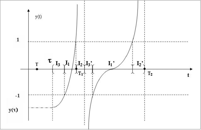
Figure 1: Riccati solution

In this case we have

$$U=I_{3}\cup I_{1}\cup I_{2}\cup I_{3}^{\prime}\cup I_{1}^{\prime}\cup I_{2}^{\prime}$$

where:

$I_{1}$ is the first interval of type $1$, after $\tau$ and before $T_{1}(\tau)$;

$I_{2}$ is the first interval of type $2$, after $\tau$ and before $T_{1}(\tau)$;

$I_{3}$ is the first interval of type $3$, after $\tau$ and before $T_{1}(\tau)$;

$I_{1}^{\prime}$ is the first interval of type $1$, after $T_{1}(\tau)$ and before $T_{2}(\tau)$;

$I_{2}^{\prime}$ is the first interval of type $2$, after $T_{1}(\tau)$ and before $T_{2}(\tau)$;

$I_{3}^{\prime}$ is the first interval of type $3$, after $T_{1}(\tau)$ and before $T_{2}(\tau)$.

We study this situation which is “the worst” it could happen. The remaining cases can be dealt with similarly and we shall skip proofs.

For $i=\{1,2,3\}$ we set $|I_{i}|=g_{i}(\tau)$ and $|I_{i}^{\prime}|=g_{i}^{\prime}(\tau)$. We are going to prove that, in the above hypotheses, each $g_{i}(\tau),\ g_{i}^{\prime}(\tau)$ is $O(\tau)$ as $\tau\to+\infty$.

We consider at first an open interval $J$ of type $3$ so that $J$ could be either $I_{3}$ or $I_{3}^{\prime}$. Set $P(\tau)<Q(\tau)$ to denote its end points; thus $g_{3}(\tau)=|J|(\tau)=Q(\tau)-P(\tau)$ and $g_{3}(\tau)$ is clearly piecewise $C^{0}([T,+\infty))$. We have $y(Q)=-1$ and $y(P)\leq-1$ if $y$ is defined in $P$, otherwise $y(P^{+})=-\infty$. As in Theorem 2.1, (4.17) yields

$$y^{\prime}\geq 2\sqrt{A(t)}|y|=2\sqrt{A(t)}(-y)\qquad\text{a.e. on }J$$

Fix $t\in(P,Q]$ and integrate on $[t,Q]$. Recalling that $y(s)\leq y(Q)=-1$ $\forall\ s\in(P,Q]$ we have

$$y(t)\leq-\exp\Big{\{}2\int_{t}^{Q}{\sqrt{A(s)}ds}\Big{\}}\qquad\forall\ t\in(P,Q]$$ (4.20)

Since $y^{\prime}/y^{2}\geq 1/v$ almost everywhere, integrating on $[P+\varepsilon,t]$ for some small $\varepsilon>0$ we obtain

$$\frac{1}{y(P+\varepsilon)}-\frac{1}{y(t)}\geq\int^{t}_{P+\varepsilon}{\frac{ds}{f(s)}}$$ (4.21)

Letting $\varepsilon\to 0^{+}$ we get

$$-\frac{1}{y(t)}\geq-\frac{1}{y(P^{+})}+\int_{P}^{t}\frac{ds}{f(s)}\geq\int_{P}^{t}\frac{ds}{f(s)}$$ (4.22)

which is valid $\forall$ $t\in(P,Q]$. Now, from (4.20) and because of (A4)

$$2\int_{t}^{Q}\sqrt{A(s)}ds\geq c\int_{t}^{Q}\frac{f^{\prime}(s)}{f(s)}ds=\log\left(\frac{f(Q)}{f(t)}\right)^{c}$$

and therefore, from (4.20),

$$-\frac{1}{y(t)}\leq\left(\frac{f(t)}{f(Q)}\right)^{c}$$

Substituting into (4.22) and using (F2) we obtain

$$1\geq\left(\frac{f(Q)}{f(t)}\right)^{c}\int_{P}^{t}\frac{ds}{f(s)}\geq(t-P)\frac{f(Q)^{c}}{f(t)^{c+1}}\quad\forall\ t\in(P,Q)$$ (4.23)

Suppose now that $J=I_{3}$, so that $P(\tau)=\tau$ and $Q(\tau)=\tau+g_{3}(\tau)$ . Since $t\in(P,Q)$, there exists $\xi\in(0,1)$ such that

$$t=\tau+(1-\xi)g_{3}(\tau)\quad,\quad t-P=(1-\xi)g_{3}(\tau)$$

and since $t$ was arbitrary, from (4.23) we obtain

$$\sup_{\xi\in(0,1)}\frac{(1-\xi)g_{3}(\tau)f(\tau+g_{3}(\tau))^{c}}{f(\tau+(1-\xi)g_{3}(\tau))^{c+1}}\leq 1$$ (4.24)

in this case it follows that $g_{3}\in{\cal A}(f,0,c)$ and then $g_{3}(\tau)=O(\tau)$ as $\tau\to+\infty$.
We will deal with the case $J=I_{3}^{\prime}$ later.

Next, we consider an interval $J$ of type $1$. Set $P(\tau)<Q(\tau)$ to denote its end points; thus $g_{1}(\tau)=|J|(\tau)=Q(\tau)-P(\tau)$ and $g_{1}(\tau)$ is piecewise $C^{0}([T;+\infty))$. In this case $y(P)=-1$, $y(Q)=1$ and $|y|\leq 1$ on $J$. We integrate Riccati equation (4.17) on $[P,Q]$ to obtain

$$2=\int_{P}^{Q}{y^{\prime}(s)ds}=\int_{P}^{Q}{A(s)v(s)ds}+\int_{P}^{Q}\frac{y^{2}(s)}{v(s)}ds\geq\int_{P}^{Q}A(s)v(s)ds$$

Next, without loss of generality we can suppose to have chosen $T$ sufficiently large that (V2), in particular $1/v\in L^{1}(+\infty)$, implies

$$\int_{T}^{+\infty}\frac{ds}{v(s)}\leq 1$$

so that

$$\int_{P}^{Q}\frac{ds}{v(s)}\leq 1$$

From the above inequality, using (A4) and the generalized mean value theorem it follows that, for some $T_{0}\in[P,Q]$,

$$\begin{array}[]{lcl}2&\geq&\displaystyle\int_{P}^{Q}{A(s)v(s)ds}\int_{P}^{Q}{\frac{ds}{v(s)}}\geq\int_{P}^{Q}\frac{c^{2}}{4}\left(\frac{f^{\prime}(t)}{f(t)}\right)^{2}v(s)ds\int_{P}^{Q}\frac{ds}{v(s)}\\[14.22636pt] &=&\displaystyle\frac{c^{2}}{4}\left(\frac{f^{\prime}(T_{0})}{f(T_{0})}\right)^{2}\int_{P}^{Q}{v(s)ds}\int_{P}^{Q}{\frac{ds}{v(s)}}\end{array}$$

On the other hand, from Hölder inequality

$$(Q-P)^{2}\leq\int_{P}^{Q}{v(s)ds}\int_{P}^{Q}{\frac{ds}{v(s)}}$$

so that

$$\sqrt{2}\geq\frac{c}{2}\left(\frac{f^{\prime}(T_{0})}{f(T_{0})}\right)(Q-P)$$

or, in other words, using (F1), (F2) and observing that (F4) implies that $f^{\prime}$ is eventually positive,

$$\frac{2\sqrt{2}}{c}\frac{f(T_{0})}{f^{\prime}(T_{0})}\geq Q-P$$ (4.25)

Now, if $J=I_{1}$, $P(\tau)=\tau+g_{3}(\tau)$, $Q(\tau)=P(\tau)+g_{1}(\tau)$ and there exists $\theta\in[0,1]$ such that $T_{0}=\tau+g_{3}(\tau)+\theta g_{1}(\tau)$. Substituting in (4.25) and using (F4) we obtain

$$g_{1}(\tau)\leq\frac{2\sqrt{2}}{c}\frac{f(\tau+g_{3}(\tau)+\theta g_{1}(\tau))}{f^{\prime}(\tau+g_{3}(\tau)+\theta g_{1}(\tau))}\leq\frac{2D\sqrt{2}}{c}(\tau+g_{3}(\tau)+\theta g_{1}(\tau))^{\mu}$$ (4.26)

In case $\mu\leq 0$ we immediately obtain $g_{1}(\tau)=O(\tau)$, hence we examine the case $\mu\in(0,1)$. Using the already known equality $g_{3}(\tau)=O(\tau)$ and inequality $(x+y)^{\mu}\leq x^{\mu}+y^{\mu}$, there exist constants $K_{1},K_{2}>0$ such that

$$\frac{g_{1}(\tau)}{\tau}\leq\frac{K_{1}}{\tau^{1-\mu}}+\frac{K_{2}g_{1}(\tau)^{\mu}}{\tau}.$$ (4.27)

Using a simple reasoning by contradiction, (4.27) implies $g_{1}(\tau)=O(\tau)$ as $\tau\to+\infty$.

If $J=I_{1}^{\prime}$, $P(\tau)=\tau+(g_{1}+g_{2}+g_{3})(\tau)+g_{3}^{\prime}(\tau)$, $Q(\tau)=P(\tau)+g^{\prime}_{1}(\tau)$, $T_{0}=\tau+(g_{1}+g_{2}+g_{3})(\tau)+g_{3}^{\prime}(\tau)+\theta g^{\prime}_{1}(\tau)$, and substituting into (4.25)

$$g_{1}^{\prime}(\tau)\leq\frac{2\sqrt{2}}{c}\frac{f(\tau+(g_{1}+g_{2}+g_{3})(\tau)+g_{3}^{\prime}(\tau)+\theta g_{1}^{\prime}(\tau))}{f^{\prime}(\tau+(g_{1}+g_{2}+g_{3})(\tau)+g_{3}^{\prime}(\tau)+\theta g_{1}^{\prime}(\tau))}$$ (4.28)

We will come back to this inequality later to prove $g_{1}^{\prime}(\tau)=O(\tau)$ as $\tau\to+\infty$. Indeed, by the same argument as above, the only things that remain to show for this purpose are $g_{2}(\tau)=O(\tau)$ and $g_{3}^{\prime}(\tau)=O(\tau)$ as $\tau\to+\infty$, and we are going to prove these facts now.

We consider an interval $J$ of type $2$ and again let $P(\tau)<Q(\tau)$ denote its end points. Clearly $y(P)=1$ and $y(Q)=\mu>1$ (or $y(Q^{-})=+\infty$ in case that $z(Q)=0$. Indeed, what follows works with any $\mu>0$). Again

$$y^{\prime}\geq 2\sqrt{A(t)}y\qquad\text{and}\qquad\frac{y^{\prime}}{y^{2}}\geq\frac{1}{v}\qquad\text{a.e. on }J$$

Fix $t\in[P,Q)$. Using $y(P)=1$, integration of the first inequality on $[P,t]$ yields

$$y(t)\geq\exp\Big{\{}2\int_{P}^{t}\sqrt{A(s)}ds\Big{\}}\qquad\forall\ t\in[P,Q),$$ (4.29)

while integrating the second one on $[t,Q-\varepsilon)$, for some small $\varepsilon>0$, and proceeding as in (4.21) we have

$$\frac{1}{y(t)}\geq\int_{t}^{Q}\frac{ds}{f(s)}\qquad\forall\ t\in(P,Q).$$ (4.30)

Thus, observing that

$$2\int_{P}^{t}{\sqrt{A(s)}ds}\geq\log\left(\frac{f(t)}{f(P)}\right)^{c}$$

we deduce from (4.29)

$$\frac{1}{y(t)}\leq\left(\frac{f(P)}{f(t)}\right)^{c}.$$

Finally, substituting into (4.30)

$$1\geq\left(\frac{f(t)}{f(P)}\right)^{c}\int_{t}^{Q}\frac{ds}{f(s)}\geq(Q-t)\frac{1}{f(Q)}\left(\frac{f(t)}{f(P)}\right)^{c}\quad\forall\ t\in(P,Q)$$ (4.31)

Suppose now $J=I_{2}$ so that $g_{2}(\tau)=Q(\tau)-P(\tau)$,

$$\begin{array}[]{l}P(\tau)=\tau+g_{3}(\tau)+g_{1}(\tau)\\ Q(\tau)=\tau+g_{3}(\tau)+g_{1}(\tau)+g_{2}(\tau)\end{array}$$

and since $t\in(P,Q)$, for some $\xi\in(0,1)$ we have

$$\begin{array}[]{l}t=\tau+(1-\xi)g_{2}(\tau)+g_{1}(\tau)+g_{3}(\tau)\\ Q-t=\xi g_{2}(\tau)\end{array}$$

Substituting into (4.31) yields,

$$\sup_{\xi\in(0,1)}{\frac{\xi g_{2}(\tau)f(\tau+(1-\xi)g_{2}(\tau)+g_{1}(\tau)+g_{3}(\tau))^{c}}{f(\tau+g_{2}(\tau)+g_{1}(\tau)+g_{3}(\tau))f(\tau+g_{1}(\tau)+g_{3}(\tau))^{c}}}\leq 1$$ (4.32)

Thus, setting $(g_{1}+g_{3})(\tau)=k(\tau)$ since $g_{1}(\tau)=O(\tau)$ and $g_{3}(\tau)=O(\tau)$ as $\tau\to+\infty$, we have that $k(\tau)=O(\tau)$ as $\tau\to+\infty$ and

$$g_{2}\in{\cal B}(f,k,c)$$

and so $g_{2}(\tau)=O(\tau)$ as $\tau\to+\infty$.

We can now deal with the case $J=I_{3}^{\prime}$. We have already shown that $g_{1}(\tau)+g_{2}(\tau)+g_{3}(\tau)=O(\tau)$ as $\tau\to\infty$. We go back to (4.23) with $J=I_{3}^{\prime}=(P(\tau),Q(\tau))$: note that now

$$P(\tau)=\tau+g_{3}(\tau)+g_{1}(\tau)+g_{2}(\tau)\quad,\quad Q(\tau)=P(\tau)+g_{3}^{\prime}(\tau)$$

where, obviously, $g_{3}^{\prime}(\tau)=|I_{3}^{\prime}|$. Since $t\in(P,Q)$, for some $\xi\in(0,1)$ we have

$$\begin{array}[]{l}t=\tau+(1-\xi)g_{3}^{\prime}(\tau)+(g_{3}+g_{1}+g_{2})(\tau)\\ t-P=(1-\xi)g_{3}^{\prime}(\tau)\end{array}$$

and substituting into (4.23), since $t\in(P,Q)$, is arbitrary we have

$$\sup_{\xi\in(0,1)}\frac{(1-\xi)g_{3}^{\prime}(\tau)f(\tau+g_{3}^{\prime}(\tau)+(g_{1}+g_{2}+g_{3})(\tau))^{c}}{f(\tau+(1-\xi)g_{3}^{\prime}(\tau)+(g_{1}+g_{2}+g_{3})(\tau))^{c+1}}\leq 1$$ (4.33)

Thus, setting $h(\tau)=(g_{1}+g_{2}+g_{3})(\tau)$, $h(\tau)=O(\tau)$ as $\tau\to+\infty$ and so we have $g_{3}^{\prime}\in{\cal A}(f,h,c)$ therefore $g_{3}^{\prime}(\tau)=O(\tau)$ as $\tau\to+\infty$.

Coming back to inequality (4.28), we can now claim that also $g_{1}^{\prime}(\tau)=O(\tau)$ as $\tau\to+\infty$.

The last case is $J=I_{2}^{\prime}$ so that $g_{2}^{\prime}(\tau)=Q(\tau)-P(\tau)$. Now we have

$$\begin{array}[]{l}P(\tau)=\tau+(g_{3}+g_{1}+g_{2}+g_{3}^{\prime}+g_{1}^{\prime})(\tau)\\ Q(\tau)=P(\tau)+g_{2}^{\prime}(\tau)\end{array}$$

and since $t\in(P,Q)$ there exists $\xi\in(0,1)$ such that

$$\begin{array}[]{l}t=\tau+(1-\xi)g_{2}^{\prime}(\tau)+(g_{3}+g_{1}+g_{2}+g_{3}^{\prime}+g_{1}^{\prime})(\tau)\\ Q(\tau)-t=\xi g_{2}^{\prime}(\tau)\end{array}$$

Setting $k(\tau)=(g_{3}+g_{1}+g_{2}+g_{3}^{\prime}+g_{1}^{\prime})(\tau)$, we have already proved that $k(\tau)=O(\tau)$ as $\tau\to+\infty$. Substituting into (4.31) yields

$$\sup_{\xi\in(0,1)}\frac{\xi g_{2}^{\prime}(\tau)f(\tau+(1-\xi)g_{2}^{\prime}(\tau)+k(\tau))^{c}}{f(\tau+g_{2}^{\prime}(\tau)+k(\tau))f(\tau+k(\tau))^{c}}\leq 1$$ (4.34)

Thus we have

$$g_{2}^{\prime}\in{\cal B}(f,k,c)$$

therefore $g_{2}^{\prime}(\tau)=O(\tau)$ as $\tau\to+\infty$, and this shows that

$$T_{2}(\tau)-T_{1}(\tau)\leq T_{2}(\tau)-\tau=(g_{3}+g_{1}+g_{2}+g_{3}^{\prime}+g_{1}^{\prime}+g_{2}^{\prime})(\tau)=O(\tau)$$

as $\tau\to+\infty$, so we have the first part of the theorem, that is, (4.15).

To conclude, we shall estimate the quantity

$$K=\limsup_{\tau\to+\infty}\frac{T_{2}(\tau)-\tau}{\tau}.$$

Looking at the group of equations (4.24), (4.26), (4.32), (4.33), (4.28) and (4.34), we first note that each of the functions $g_{i}(\tau)$ and $g_{i}^{\prime}(\tau)$ involved in the proof (shortly $g(\tau)$) satisfies one of the following inequalities, for $\tau\geq T$ and for some suitable function $h(\tau)$ which is known to be $O(\tau)$:

$$\displaystyle\sup_{\xi\in(0,1)}\frac{(1-\xi)g(\tau)f(\tau+g(\tau)+h(\tau))^{c}}{f(\tau+(1-\xi)g(\tau)+h(\tau))^{c+1}}\leq 1 \quad{\rm for}\ g_{3}\ {\rm and}\ g_{3}^{\prime}$$ (4.35)

$$\displaystyle g(\tau)\leq\frac{2\sqrt{2}}{c}\frac{f(\tau+h(\tau)+\theta g(\tau))}{f^{\prime}(\tau+h(\tau)+\theta g(\tau))} \quad{\rm for}\ g_{1}\ {\rm and}\ g_{1}^{\prime}$$ (4.36)

$$\displaystyle\sup_{\xi\in(0,1)}\frac{\xi g(\tau)f(\tau+(1-\xi)g(\tau)+h(\tau))^{c}}{f(\tau+g(\tau)+h(\tau))\cdot f(\tau+h(\tau))^{c}}\leq 1 \quad{\rm for}\ g_{2}\ {\rm and}\ g_{2}^{\prime}$$ (4.37)

For the sake of simplicity, we perform computations in case

$$f(t)=\Lambda\exp\{at^{\alpha}\},\qquad a,\Lambda,\alpha>0\quad$$

(note that $f$ satisfy property $(P)$ for every $c>1$). We shall determine $K$ by computing, in each of the tree cases above,

$$K_{j}=\limsup_{\tau\to+\infty}\frac{g(\tau)}{\tau}\qquad$$

(the index $j$ corresponds to the cases satisfied by $g_{j}$ and $g_{j}^{\prime}$), and then summing the terms ”inductively” following the changes of the known function $h$ case by case. For this purpose let

$$H\geq\limsup_{\tau\to+\infty}\frac{h(\tau)}{\tau}$$

Consider at first inequality (4.36): we immediately find that, for this choice of $f$,

$$\frac{g(\tau)}{\tau}\leq\frac{2\sqrt{2}}{c}\frac{1}{\tau}\frac{1}{a\alpha(\tau+h(\tau)+\theta g(\tau))^{\alpha-1}}\leq\frac{2\sqrt{2}}{ca\alpha}\frac{\big{(}1+\frac{h(\tau)}{\tau}+\frac{g(\tau)}{\tau}\big{)}^{1-\alpha}}{\tau^{\alpha}}$$

We claim that $K_{1}=0$. Indeed, suppose by contradiction that there exists a divergent sequence $\{\tau_{n}\}$ such that $g(\tau_{n})/\tau_{n}\rightarrow K_{1}>0$. Then, evaluating the above inequality along $\{\tau_{n}\}$ and passing to the limit we reach

$$0<K_{1}\leq 0\qquad\mathrm{a\ contradiction.}$$

We now focus our attention on (4.35). By an algebraic manipulation

$$g(\tau)\leq\frac{1}{1-\xi}\frac{f(\tau+(1-\xi)g(\tau)+h(\tau))^{c+1}}{f(\tau+g(\tau)+h(\tau))^{c}}\quad\forall\ \xi\in(0,1)\ .$$

Due to the form of $f$, better estimates can be obtained choosing $\xi$ near $1$. For $\tau>1$, we choose $\xi=(\tau-1)/\tau$. For the ease of notation let $x(\tau)=g(\tau)/\tau$, so that $x(\tau)$ is bounded on $[T,+\infty)$ because $f$ satisfies property $(P)$. With this choice of $\xi$ we have

$$x(\tau)\leq\frac{f(\tau+x(\tau)+h(\tau))^{c+1}}{f(\tau+\tau x(\tau)+h(\tau))^{c}},$$ (4.38)

thus substituting

$$x(\tau)\leq\Lambda\exp\Big{\{}a\tau^{\alpha}\Big{[}(c+1)\Big{(}1+\frac{x(\tau)}{\tau}+\frac{h(\tau)}{\tau}\Big{)}^{\alpha}-c\Big{(}1+x(\tau)+\frac{h(\tau)}{\tau}\Big{)}^{\alpha}\Big{]}\Big{\}}$$

Suppose now that $K_{3}>0$, and evaluate this inequality along a sequence $\{\tau_{n}\}$ such that $x(\tau_{n})\to K_{3}$. Choose $0<\delta<K_{3}$, and let $n$ be large enough that the following inequalities hold:

$$x(\tau_{n})>K_{3}-\delta\quad,\quad\frac{x(\tau_{n})}{\tau_{n}}<\delta$$

This yields:

$$x(\tau_{n})\leq\Lambda\exp\Big{\{}a\tau_{n}^{\alpha}\Big{[}(c+1)\Big{(}1+\delta+\frac{h(\tau_{n})}{\tau_{n}}\Big{)}^{\alpha}-c\Big{(}1+K_{3}-\delta+\frac{h(\tau_{n})}{\tau_{n}}\Big{)}^{\alpha}\Big{]}\Big{\}}$$ (4.39)

Suppose now that $K_{3}$ satisfies

$$\max_{\mu\in[0,H]}\Big{\{}(c+1)(1+\mu)^{\alpha}-c(1+K_{3}+\mu)^{\alpha}\Big{\}}<0,$$ (4.40)

and compare it with (4.39). We can say that, by continuity, there exists a small $\delta>0$ such that the expression between square brackets is strictly less than $0$. Letting now $\tau_{n}$ go to infinity in (4.39) we deduce $0<K_{3}\leq 0$, a contradiction. Note that (4.40) holds if and only if

$$(c+1)-c\Big{(}\frac{K_{3}}{\mu+1}+1\Big{)}^{\alpha}<0\qquad\forall\ \mu\in[0,H],$$

that is,

$$K_{3}>\Big{[}\Big{(}\frac{c+1}{c}\Big{)}^{\frac{1}{\alpha}}-1\Big{]}(1+H).$$

Hence, if $K_{3}>0$, we necessarily have

$$K_{3}\leq\Big{[}\Big{(}\frac{c+1}{c}\Big{)}^{\frac{1}{\alpha}}-1\Big{]}(1+H).$$ (4.41)

The same technique can be exploited when dealing with (4.37): from

$$g(\tau)\leq\frac{1}{\xi}\frac{f(\tau+g(\tau)+h(\tau))\cdot f(\tau+h(\tau))^{c}}{f(\tau+(1-\xi)g(\tau)+h(\tau))^{c}}\qquad\forall\ \xi\in(0,1)$$ (4.42)

we deduce that it is better to choose $\xi$ near 0, so we set $\xi=1/\tau$ and we obtain, with the same notations,

$$x(\tau)\leq\frac{f(\tau+\tau x(\tau)+h(\tau))\cdot f(\tau+h(\tau))^{c}}{f(\tau+(\tau-1)x(\tau)+h(\tau))^{c}}$$

Thus

$$\begin{array}[]{lcl}x(\tau)&\leq&\Lambda\exp\Big{\{}a\tau^{\alpha}\Big{[}\Big{(}1+x(\tau)+\frac{h(\tau)}{\tau}\Big{)}^{\alpha}+\\[11.38092pt] &&+c\Big{(}1+\frac{h(\tau)}{\tau}\Big{)}^{\alpha}-c\Big{(}1+\frac{\tau-1}{\tau}x(\tau)+\frac{h(\tau)}{\tau}\Big{)}^{\alpha}\Big{]}\Big{\}}\end{array}$$

Next, if $K_{2}>0$ we choose a sequence $\{\tau_{n}\}$ realizing $K_{2}$ and we consider $n$ sufficiently large that

$$\frac{(\tau_{n}-1)}{\tau_{n}}>(1-\delta)\quad,\quad K_{2}-\delta<x(\tau_{n})<K_{2}+\delta$$

obtaining the estimate

$$\begin{array}[]{lcl}x(\tau_{n})&\leq&\Lambda\exp\Big{\{}a\tau_{n}^{\alpha}\cdot\Big{[}\Big{(}1+(K_{2}+\delta)+\frac{h(\tau_{n})}{\tau_{n}}\Big{)}^{\alpha}+\\[11.38092pt] &&+c\Big{(}1+\frac{h(\tau_{n})}{\tau_{n}}\Big{)}^{\alpha}-c\Big{(}1+(1-\delta)(K_{2}-\delta)+\frac{h(\tau_{n})}{\tau_{n}}\Big{)}^{\alpha}\Big{]}\Big{\}}\end{array}$$ (4.43)

Now, if $K_{2}$ satisfies

$$\max_{\mu\in[0,H]}\Big{\{}(1+K_{2}+\mu)^{\alpha}+c(1+\mu)^{\alpha}-c(1+K_{2}+\mu)^{\alpha}\Big{\}}<0,$$ (4.44)

we reach a contradiction proceeding as in the previous case. Similarly to what we did above this yields the bound

$$K_{2}\leq\Big{[}\Big{(}\frac{c}{c-1}\Big{)}^{\frac{1}{\alpha}}-1\Big{]}(1+H)$$ (4.45)

To simplify the writing we now set

$$W=\Big{[}\Big{(}\frac{c+1}{c}\Big{)}^{\frac{1}{\alpha}}-1\Big{]}\quad,\quad Z=\Big{[}\Big{(}\frac{c}{c-1}\Big{)}^{\frac{1}{\alpha}}-1\Big{]}$$

To estimate $g_{3}(\tau)/\tau$, we shall use (4.41) and, from (4.24), we deduce $h(\tau)\equiv 0$ and thus $H=0$. Therefore, we get

$$K_{3}\leq W.$$

We have already shown that $K_{1}=0$. Next, to estimate $g_{2}(\tau)/\tau$ we shall consider (4.45). By (4.32) $h(\tau)=g_{3}(\tau)+g_{1}(\tau)$, so we can use for $H$ the sum $W+0=W$, hence

$$K_{2}\leq Z(1+W).$$

Proceeding along the same lines we obtain the estimates

$$\begin{array}[]{l}K_{3}^{\prime}\leq W\big{(}1+W+Z(1+W)\big{)};\\[5.69046pt] K_{1}^{\prime}=0;\\[5.69046pt] K_{2}^{\prime}\leq Z\Big{(}1+W+Z(1+W)+W\big{(}1+W+Z(1+W)\big{)}\Big{)}.\end{array}$$

Summing up the $K_{j}$ and the $K_{j}^{\prime}$, we obtain the surprisingly simple expression

$$K\leq\sum_{j=1}^{3}(K_{j}+K_{j}^{\prime})=\big{(}W+1\big{)}^{2}\big{(}Z+1\big{)}^{2}-1=\Big{(}\frac{c+1}{c-1}\Big{)}^{\frac{2}{\alpha}}-1\quad.$$

Thus we eventually have

$$\limsup_{\tau\to+\infty}\frac{T_{2}(\tau)}{\tau}\leq\Big{(}\frac{c+1}{c-1}\Big{)}^{\frac{2}{\alpha}}$$ (4.46)

With few modifications in the computations, it can be seen that, considering $f(t)=\Lambda\exp[at^{\alpha}\log^{\beta}t]$ instead of the above, the value of the constant $K$ does not change. $\blacktriangle$

Remark 4.2.

Since $f(t)=\Lambda\exp\{at^{\alpha}\log^{\beta}t\}$ satisfies property $(P)$ for every $c>1$, in this case conditions (A3) and (A4) may be replaced by

$$\sqrt{A(t)}\geq c\Big{(}\frac{a\alpha}{2}\Big{)}t^{\alpha-1}\log^{\beta}t\qquad\text{a.e. on }[T,+\infty),\text{ for some }c>1.$$ (A3 + A4)

Note that the right hand side of the above expression is asymptotic to $c\sqrt{\widetilde{\chi}_{f}(r)}$, hence to $c\sqrt{\chi_{f}(t)}$ by (4.4). Indeed, choose $\varepsilon>0$ such that $\overline{c}=c-2\varepsilon>1$. Then, there exists $T>0$ such that, on $[T,+\infty)$,

$$c\Big{(}\frac{a\alpha}{2}\Big{)}t^{\alpha-1}\log^{\beta}t\geq(c-\varepsilon)\sqrt{\chi_{f}(t)}\geq(c-2\varepsilon)\sqrt{\widetilde{\chi}_{f}(t)}=\overline{c}\sqrt{\widetilde{\chi}_{f}(t)},$$

hence (A4) is satisfied with $\overline{c}$. Moreover, $(iv)$ of Proposition 2.5 and $\chi_{f}(t)\geq\chi(t)$ ensure condition (A3). Applying Theorem 4.1 with $\overline{c}$ yields

$$\limsup_{\tau\rightarrow+\infty}\frac{T_{2}(\tau)}{\tau}=\Big{(}\frac{\overline{c}+1}{\overline{c}-1}\Big{)}^{\frac{2}{\alpha}}$$

Since $\varepsilon$ is arbitrary, we conclude the validity of (4.16) under assumption (A3 + A4).

Remark 4.3.

One might ask if varying the choice of the level sets in (4.19) one could obtain better estimates. It is not hard to see that, for every choice of the level, (4.46) does not change.

5 Geometric applications

This section is devoted to the proofs of the geometric applications given in the Introduction, which follow from the results of sections 2 and 4. The core are Theorems 1.4 and 1.6, where the Cauchy problems (2.2), (2.19) appear in order to obtain suitable radial test functions which yield estimates for the Rayleigh quotients of $L$ and $\Delta$ respectively. An almost direct use of Theorem 1.4 proves Theorems 1.9, 1.10 and 1.14, while Theorem 1.11 requires some special attention and further work.

5.1 The index of $\Delta+a(x)$: proof of Theorem 1.4

Choose $v(t)=\mathrm{Vol}(\partial B_{t})$. From Proposition 1.2 it follows that the spherical mean $A(t)$ belongs to $L^{\infty}_{\mathrm{loc}}([0,+\infty))$, the validity of (V1) and the existence of a locally Lipschitz solution of (2.2) whose zeros (if any) are isolated (Theorems 6.1 and 6.3 of the Appendix). Consider problem (2.2), and note that, by the coarea formula,

$$0<\int_{0}^{R_{0}}A(s)v(s)ds=\int_{0}^{R_{0}}\Big{(}\int_{\partial B_{s}}a\Big{)}ds=\int_{B_{R_{0}}}a.$$

By Corollary 2.3, assumption $(i)$ guarantees the existence of a first zero of every locally Lipschitz solution $z(t)$, whereas Corollary 2.4 implies that assumption $(ii)$ forces $z(t)$ to be oscillatory. Note that a different choice of $R$ in assumption $(ii)$ does not affect the value of the “limsup”.

We now consider case $(i)$: choose a locally Lipschitz solution $z(t)$ of (2.2), and denote with $T$ its first zero. Define

$$\psi(x)=z(r(x))$$

so that

$$\psi\in\mathrm{Lip}(\overline{B}_{T})\quad,\quad\psi\equiv 0\quad\text{on }\partial B_{T}\quad,\quad\nabla\psi(x)=z^{\prime}(r(x))\nabla r(x)\quad\text{a.e. on }M$$

and fix $0<\varepsilon<T$. Then, using the coarea formula, Gauss lemma and (2.2) we obtain

$$\begin{array}[]{l}\displaystyle\int_{B_{T}\backslash B_{\varepsilon}}|\nabla\psi|^{2}-a(x)\psi^{2}=\int_{B_{T}\backslash B_{\varepsilon}}|\nabla\psi|^{2}-A(r)\psi^{2}\\[11.38092pt] =\displaystyle\int_{\varepsilon}^{T}(z^{\prime}(r))^{2}v(r)dr-\int_{\varepsilon}^{T}A(r)z^{2}(r)v(r)dr\\[11.38092pt] =\displaystyle-z(\varepsilon)z^{\prime}(\varepsilon)v(\varepsilon)-\int_{\varepsilon}^{T}z(r)\big{[}(v(r)z^{\prime}(r))^{\prime}+A(r)v(r)z(r)\big{]}=-z(\varepsilon)z^{\prime}(\varepsilon)v(\varepsilon)\end{array}$$

and letting $\varepsilon\downarrow 0^{+}$ we deduce

$$\int_{B_{T}}|\nabla\psi|^{2}-a(x)\psi^{2}\leq 0.$$

By Rayleigh characterization of eigenvalues and by domain monotonicity we conclude $\lambda_{1}^{L}(M)<0$.

Suppose now we are in case $(ii)$, and assume by contradiction that there exists $R>0$ such that

$$\lambda_{1}^{L}(M\backslash B_{R})\geq 0.$$ (5.1)

As already stressed in the Introduction, by a result of Fisher-Colbrie [FC], if the index of $L$ is finite then (5.1) holds for a sufficiently large $R$.

In our assumptions, every locally Lipschitz solution $z(t)$ of (2.19) is oscillatory. Let $T_{1}<T_{2}$ be two consecutive zeros of $z(t)$ strictly after $R$. Define $\psi(x)=z(r(x))$ in the annular region $B_{T_{2}}\backslash B_{T_{1}}$, and $\psi(x)\equiv 0$ in the rest of $M$. Then $\psi\in\mathrm{Lip}_{0}(M)$ with support contained in $M\backslash B_{R}$. Proceeding as in the previous case, we obtain

$$\int_{B_{T_{2}}\backslash B_{T_{1}}}|\nabla\psi|^{2}-a(x)\psi^{2}\leq 0,$$

hence, by strict domain monotonicity, $\lambda_{1}(M\backslash B_{R})<0$, contradicting (5.1).

Let us finally consider case $(iii)$. By Remark 4.2 and Theorem 4.1, (2.2) is oscillatory, thus $L$ is unstable at infinity. In particular, the index of $L$ is infinite. Note that (1.13) is equivalent to prove that

$$\liminf_{r\rightarrow+\infty}\frac{\mathrm{ind}_{L}(B_{r})}{\log r}\geq\frac{1}{\log K}\quad,\quad\mathrm{with}\quad K=\Big{(}\frac{c+1}{c-1}\Big{)}^{\frac{2}{\alpha}}.$$

Fix $\varepsilon>0$. Then, by Theorem 4.1 there exists $T=T(\varepsilon)$ such that on $[T,+\infty)$

$$\frac{T_{2}(r)}{r}\leq K_{\varepsilon}=\Big{(}\frac{c+1}{c-1}\Big{)}^{\frac{2}{\alpha}}+\varepsilon.$$

Proceeding as above, on $M\backslash B_{r}$ we can find a radial function $\psi_{1}(x)$, with support contained in $B_{K_{\varepsilon}r}$, which makes the Rayleigh quotient non positive. Starting from $T_{2}(r)$, the second zero after $T_{2}(r)$ is attained before $K_{\varepsilon}T_{2}(r)\leq K_{\varepsilon}^{2}r$, and we can construct a new Lipschitz radial function $\psi_{2}(x)$ which makes the Rayleigh quotient non positive. Moreover, the support of $\psi_{2}$ is disjoint from that of $\psi_{1}$. In conclusion, the index of $L$ grows at least by $1$ when the radius is multiplied by $K_{\varepsilon}$, hence

$$\mathrm{ind}_{L}(B_{r})\geq\mathrm{ind}_{L}(B_{T})+\Big{\lfloor}\log_{K_{\varepsilon}}\Big{(}\frac{r}{T}\Big{)}\Big{\rfloor},$$

where $\lfloor s\rfloor$ denotes the floor of $s$. Therefore we have

$$\liminf_{r\rightarrow+\infty}\frac{\mathrm{ind}_{L}(B_{r})}{\log_{K_{\varepsilon}}r}\geq 1\qquad\forall\ \varepsilon>0.$$ (5.2)

From the change of base theorem, for every $u,v>1$, $r>0$

$$\frac{\log_{u}r}{\log_{v}r}=\log_{u}v=\frac{\log v}{\log u},$$ (5.3)

so that

$$\liminf_{r\rightarrow+\infty}\frac{\mathrm{ind}_{L}(B_{r})}{\log r}\geq\frac{1}{\log K_{\varepsilon}}\qquad\forall\ \varepsilon>0.$$ (5.4)

Letting $\varepsilon\rightarrow 0$ yields the desired conclusion. $\blacktriangle$

5.2 Tangent envelopes: proof of Theorem 1.9

We briefly recall some well known facts. Suppose we are given an isometrically immersed hypersurface

$$\varphi:M^{m}\longrightarrow N^{m+1},$$

where $N$ is orientable. We fix the index notation $i,j,k,t\in\{1,\ldots,m\}$, and we choose a local Darboux frame $\{e_{i},\nu\}$. Let $R,\mathrm{Ricc},s$ (resp $\overline{R},\overline{\mathrm{Ricc}},\overline{s}$) be the curvature tensor, the Ricci tensor and the scalar curvature of $M$ (resp. $N$), denote with $II=(h_{ij})$ the second fundamental form of the immersion, with $|II|^{2}$ the square of its Hilbert-Schmidt norm and with $H=m^{-1}h_{ii}\nu$ the mean curvature vector. Tracing twice the Gauss equations

$$R_{ijkt}=\overline{R}_{ijkt}+h_{ik}h_{jt}-h_{it}h_{jk}$$ (5.5)

we get

$$s=\overline{s}-2\overline{\mathrm{Ricc}}(\nu,\nu)+m^{2}|H|^{2}-|II|^{2}.$$ (5.6)

Moreover, we recall the Codazzi-Mainardi equation

$$h_{ijk}-h_{ikj}=\overline{R}^{m+1}_{ijk},$$ (5.7)

where $(h_{ijk})$ are the components of the covariant derivative $\nabla II$. A minimal immersion $\varphi$ is characterized by $H\equiv 0$, which implies that $\varphi$ is a stationary point for the volume functional on every relatively compact domain with smooth boundary in $M$. It is known that if, for example, $N=\mathbb{R}^{m+1}$, a minimal hypersurface cannot be compact and, by (5.6), $s(x)=-|II|^{2}\leq 0$.
We say that $\varphi$ is stable if it locally minimizes the volume functional up to second order, and unstable otherwise. Analytically the condition of stability is expressed by

$$\int_{M}|\nabla\psi|^{2}-\big{(}|II|^{2}+\overline{\mathrm{Ricc}}(\nu,\nu)\big{)}\psi^{2}\geq 0\qquad\forall\ \ \psi\in C^{\infty}_{0}(M)$$

and it is equivalent to the fact that the Schrödinger operator $L=\Delta+|II|^{2}+\overline{\mathrm{Ricc}}(\nu,\nu)$ satisfies $\lambda_{1}^{L}(M)\geq 0$. Observe that, if $N$ is Ricci flat (for example, $N=\mathbb{R}^{m+1}$), using (5.6) we get

$$L=\Delta+|II|^{2}=\Delta-s(x).$$

The strategy of the proof of Theorem 1.9 is to proceed by contradiction. First we prove that, if (1.27) fails, $M$ is stable at infinity, i.e. $\lambda_{1}^{L}(M\backslash\Omega)\geq 0$ for the chosen compact domain $\Omega$; then, we contradict this fact using Theorem 1.4 under assumptions (1.23) or (1.24), (1.25), (1.26).

Proof (of Theorem 1.9). We reason by contradiction and, without loss of generality, we can assume that the origin $o$ of $\mathbb{R}^{m+1}$ belongs to

$$\mathbb{R}^{m+1}\backslash\bigcup_{x\in M\backslash\Omega}T_{x}M.$$

Consider on $M\backslash\Omega$ a local normal unit vector field $\nu$ and define the local vector field $X=\langle\varphi,\nu\rangle\nu$, where $\langle,\rangle$ denotes the canonical metric on $\mathbb{R}^{m+1}$. For every point $x$ in the domain of $X$ we have $X_{x}\not\equiv 0$ since otherwise $\varphi(x)$ would be orthogonal to $\nu(x)$ and thus $T_{x}M$ would contain the origin $o$. Moreover, under a change of Darboux frame the value of $X$ does not change, hence it provides a globally defined, nowhere vanishing normal vector field, proving that $M\backslash\Omega$ is orientable. Define $u(x)=\langle\varphi(x),\nu(x)\rangle\neq 0$, $u\in C^{\infty}(M\backslash\Omega)$. Possibly inverting the orientation on connected components, we can suppose $u>0$ on $M\backslash\Omega$. A simple computation using minimality of $\varphi$ and Codazzi equation (5.7) for $N=\mathbb{R}^{m+1}$ shows that $u$ is a positive solution of

$$\Delta u-s(x)u=0\qquad\mathrm{on\ }M\backslash\Omega,$$

By the result of Fisher-Colbrie and Schoen [FCS] it follows that $L=\Delta-s(x)$ has non negative spectral radius $\lambda_{1}^{L}(M\backslash\Omega)$, hence $M$ is stable at infinity.
To contradict this latter result, we choose $A(r)=-S(r)$ and we use Theorem 1.4, case $(ii)$. A contradiction is immediate in case of (1.23), while if we assume $(\mathrm{Vol}(\partial B_{r}))^{-1}\in L^{1}(+\infty)$ we can apply Proposition 2.5, item $(iv)$: indeed, under assumptions (1.24), (1.25) and (1.26), observing that

$$\frac{d}{ds}(-s^{1-\alpha}\exp\{-s^{\alpha}\})\leq\widetilde{C}\exp\{-s^{\alpha}\}\qquad\text{for }s\geq 1,$$

for some $\widetilde{C}>0$, there exist positive constants $D$ and $H$ such that

$$\begin{array}[]{lcl}\displaystyle\liminf_{r\rightarrow+\infty}\frac{\int_{R}^{r}\sqrt{A(s)}ds}{-\frac{1}{2}\log\int_{r}^{+\infty}\frac{ds}{\mathrm{Vol}(\partial B_{s})}}&\geq&\displaystyle\liminf_{r\rightarrow+\infty}\frac{\int_{R}^{r}\sqrt{C}s^{-\mu/2}ds}{-\frac{1}{2}\log\int_{r}^{+\infty}\frac{\exp\{-s^{\alpha}\}}{\Lambda}ds}\\[17.07182pt] &\geq&\displaystyle\liminf_{r\rightarrow+\infty}\Big{(}Dr^{1-\frac{\mu}{2}-\alpha}\log^{-H}r\Big{)}=+\infty.\end{array}$$

Proposition 2.5 item $(iv)$ implies (1.11), so that Theorem 1.4 case $(ii)$ contradicts the stability at infinity of $L$. $\blacktriangle$

Remark 5.3.

Obviously, when $\Omega=\emptyset$ there is a version of the above theorem in finite form, which is based on case $(i)$ of Theorem 1.4. We have preferred not to make the proposition too cumbersome, in order to better appreciate the result itself. Nevertheless, even this case seems interesting: inequality (1.9) implies that a strongly negative scalar curvature on a compact set spreads the tangent hyperplanes everywhere on $\mathbb{R}^{m+1}$, independently of the behavior of the curvature outside the compact.

5.4 The Gauss map: proof of Theorem 1.10

The proof follows the same lines of Theorem 1.9, and we maintain the same notations. We fix an equator $E$ and we reason by contradiction: assume that there exist a sufficiently large geodesic ball $B_{R}$ such that, outside $B_{R}$, $\nu$ does not meet $E$. In other words $\nu(M\backslash B_{R})$ is contained in the open spherical cups determined by $E$. Indicating with $w\in\mathbb{S}^{m}$ one of the two focal points of $E$, we can say that $\langle w,\nu(x)\rangle\neq 0$ for every $x\in M\backslash B_{R}$, where $\langle,\rangle$ stands for the scalar product of unit vectors in $\mathbb{S}^{m}\subset\mathbb{R}^{m+1}$. Then, the normal vector field $X=\langle w,\nu\rangle\nu$ is globally defined and nowhere vanishing on $M\backslash B_{R}$, proving that $M\backslash B_{R}$ is orientable. Therefore, the Gauss map is globally defined on $M\backslash B_{R}$. Let $\mathcal{C}$ be one of the (finitely many) connected components of $M\backslash B_{R}$; then, $\nu(\mathcal{C})$ is contained in only one of the open spherical caps determined by $E$. Up to replacing $w$ with $-w$, we can suppose $u=\langle w,\nu\rangle>0$ on $\mathcal{C}$. Proceeding in the same way for every connected component, we can construct a positive function $u$ on $M\backslash B_{R}$. By a standard calculation $u$ satisfies

$$\Delta u=-h_{ikk}\langle e_{i},w\rangle-|II|^{2}u\qquad{\rm on}\ M\backslash B_{R}.$$ (5.8)

Using Schwarz symmetry, Codazzi equation (5.7) and minimality we deduce

$$h_{ikk}=h_{kik}=h_{kki}=0,$$

hence $\Delta u+|II|^{2}u=0$. From (5.6) we get

$$\Delta u-s(x)u=0$$ (5.9)

In particular, (5.9) implies $\lambda_{1}^{L}(M\backslash B_{R})\geq 0$, where $L=\Delta-s(x)$. Observe that $s(x)=-|II|^{2}\leq 0$, so that its spherical mean $S(r)$ is non positive. As in the proof of Theorem 1.9, the assumptions imply case $(ii)$ of Theorem 1.4, and this contradicts $\lambda_{1}^{L}(M\backslash B_{R})\geq 0$. $\blacktriangle$

5.5 The Yamabe Problem: proof of Theorem 1.14

Applying Theorem 1.4 to the operator $L=\Delta-\frac{1}{c_{m}}s(x)$ we obtain $\lambda_{1}^{L}(M)<0$. Hence, the conclusion follows from Theorems $2.4$ and $2.1$ of [PRS], with the observation after Theorem $2.3$ therein. $\blacktriangle$

Remark 5.6.

We can state an alternative version at infinity of condition (1.31) via Proposition 2.5, $(iv)$. This reads as follows. Suppose that

$$S(r)\leq-\frac{H}{r^{\beta}}\qquad\mathrm{for}\ r\gg 1\ \mathit{and\ some\ }H>0,\ \beta\leq 2.$$

Then, condition

$$\sqrt{H\frac{m-2}{m-1}}>\left\{\begin{array}[]{ll}\displaystyle\liminf_{r\rightarrow+\infty}\Big{(}\frac{\frac{\beta}{2}-1}{r^{-\beta/2+1}}\log\int_{r}^{+\infty}\frac{ds}{\mathrm{Vol}(\partial B_{s})}\Big{)}&\quad\mathit{if\ }\beta<2\\[17.07182pt] \displaystyle\liminf_{r\rightarrow+\infty}\Big{(}-\frac{1}{\log r}\log\int_{r}^{+\infty}\frac{ds}{\mathrm{Vol}(\partial B_{s})}\Big{)}&\quad\mathit{if\ }\beta=2\end{array}\right.$$ (5.10)

implies the existence of the desired conformal deformation.

5.7 Minimal surfaces: proof of Theorems 1.11 and 1.13

We will obtain both the results as easy consequences of the next two lemmas, the first of which is a somewhat modified version of a result of Colding and Minicozzi [CM]. We adopt the notations of Theorems 1.9 and 1.10.

Lemma 5.8.

Let $\varphi:M^{2}\rightarrow N^{3}$ be a simply connected, minimally immersed surface in an ambient $3$-manifold. Assume that the Ricci tensor of $N$ satisfies

$$\overline{\mathrm{Ricc}}\geq 0.$$ (5.11)

Suppose that $M$ has a pole $o$, and let $L$ be the stability operator. If $\lambda_{1}^{L}(M\backslash\Omega)\geq 0$ for some compact set $\Omega$, then there exists a constant $C>0$ such that

$$\mathrm{Vol}(B_{R})\leq CR^{2}\qquad\forall\ R\geq 0.$$

Proof. Let $K$ be the sectional curvature of $M$. Since for surfaces $s(x)=2K$, using (5.11) in (5.6) yields

$$\begin{array}[]{lcl}2K&=&\displaystyle\overline{\mathrm{Ricc}}(e_{1},e_{1})+\overline{\mathrm{Ricc}}(e_{2},e_{2})-\overline{\mathrm{Ricc}}(\nu,\nu)-|II|^{2}\\[5.69046pt] &\geq&-\overline{\mathrm{Ricc}}(\nu,\nu)-|II|^{2}\end{array}$$

hence the Rayleigh quotient for the stability operator do not exceed that for $\overline{L}=\Delta-2K$. It follows that, for every subset $D\subset M$, we have inequality

$$\lambda_{1}^{L}(D)\leq\lambda_{1}^{\overline{L}}(D),$$ (5.12)

thus by the assumptions $\lambda_{1}^{\overline{L}}(M\backslash B_{R_{0}})\geq 0$ for some $R_{0}$ sufficiently large that $\Omega\subset B_{R_{0}}$.
Since $M$ is simply connected and has a pole, the geodesic spheres centered at $o$ are smooth and the geodesic balls are diffeomorphic to Euclidean ones. By Gauss-Bonnet theorem together with the first variation formula, we have

$$\int_{B_{r}}K=2\pi-l^{\prime}(r),$$ (5.13)

where $l(r)$ is the length of $\partial B_{r}$ (another way to derive this formula can be found in [PRS1], page $238$). Denote with $K(r)=\int_{B_{r}}K$, and observe that, by the coarea formula $K^{\prime}(r)=\int_{\partial B_{r}}K$.
By the stability of $\overline{L}$, for every $\psi\in\mathrm{Lip}_{0}(M\backslash B_{R_{0}})$ we have

$$\int_{M\backslash B_{R_{0}}}|\nabla\psi|^{2}+2\int_{M\backslash B_{R_{0}}}K\psi^{2}\geq 0.$$ (5.14)

Fix $R>R_{0}+2$ and choose $\psi(x)=f(r(x))$, where

$$f(t)=\left\{\begin{array}[]{ll}0&\mathrm{if\ }t\leq R_{0}\\[2.84544pt] \displaystyle t-R_{0}&\mathrm{if\ }t\in[R_{0},R_{0}+1]\\[2.84544pt] \displaystyle\frac{R-t}{R-R_{0}-1}&\mathrm{if\ }t\in[R_{0}+1,R]\\[2.84544pt] 0&\mathrm{if\ }t\geq R\end{array}\right.$$

Then, using (5.13) into (5.14) and integrating by parts, by the properties of $f$ we have

$$0\leq\int_{R_{0}}^{R}(f^{\prime}(r))^{2}l(r)dr+2\int_{R_{0}}^{R}l^{\prime}(r)(f^{2}(r))^{\prime}dr$$

Inserting the explicit expression of $f$ we obtain

$$\begin{array}[]{l}\displaystyle 0\leq\mathrm{Vol}(B_{R_{0}+1})-\mathrm{Vol}(B_{R_{0}})+\frac{\mathrm{Vol}(B_{R})-\mathrm{Vol}(B_{R_{0}+1})}{(R-R_{0}-1)^{2}}+4l(R_{0}+1)+\\[8.5359pt] \displaystyle-4\big{(}\mathrm{Vol}(B_{R_{0}+1})-\mathrm{Vol}(B_{R_{0}})\big{)}+\frac{4l(R_{0}+1)}{R-R_{0}-1}-\frac{4\big{(}\mathrm{Vol}(B_{R})-\mathrm{Vol}(B_{R_{0}+1})\big{)}}{(R-R_{0}-1)^{2}}\end{array}$$

Therefore, there exists a constant $C=C(R_{0})$ depending on the geometry of $B_{R_{0}+1}$ such that, for every $R>R_{0}+2$,

$$\frac{3\big{(}\mathrm{Vol}(B_{R})-\mathrm{Vol}(B_{R_{0}+1})\big{)}}{(R-R_{0}-1)^{2}}\leq C(R_{0})$$

hence,

$$\mathrm{Vol}(B_{R})\leq\mathrm{Vol}(B_{R_{0}+1})+\frac{C(R_{0})}{3}(R-R_{0}-1)^{2}\leq\widetilde{C(R_{0})}R^{2}.$$

Since near $o$ the geometry of $M$ is “nearly” Euclidean, up to enlarging the constant the same estimate holds on all of $M$, and this concludes the proof. $\blacktriangle$

Remark 5.9.

Note that, in case $\Omega=\emptyset$ and $N=\mathbb{R}^{3}$, we recover Colding and Minicozzi theorem, for which the simply-connectedness assumption is unnecessary: in fact, we can pass to the Riemannian universal covering $\widetilde{M}$ of $M$. Indeed, by Fisher-Colbrie and Schoen result [FCS] stability is equivalent to the existence of a positive solution $u$ of $Lu=0$ on $M$; $u$ can be lifted up by composition with the covering projection, which is a local isometry, yielding a positive solution of the same equation on $\widetilde{M}$. Moreover, in this case the existence of a pole is automatically satisfied since by (5.5) $M$ has non positive sectional curvature.

The next Lemma is a calculus exercise (see [RS]).

Lemma 5.10.

$$\mathit{If}\quad\frac{r}{\mathrm{Vol}(B_{r})}\not\in L^{1}(+\infty)\quad,\quad\mathit{then}\quad\frac{1}{\mathrm{Vol}(\partial B_{r})}\not\in L^{1}(+\infty).$$

Now we are ready to prove Theorem 1.11 and Corollary 1.13.

Proof (of Theorem 1.11). By assumption there exists a relatively compact set $\Omega$ such that $M\backslash\Omega$ is stable, that is, $\lambda_{1}^{L}(M\backslash\Omega)\geq 0$. Moreover, by Gauss equation (5.5) we get $2K=-|II|^{2}\leq 0$, so that every point of $M$ is a pole. Lemma 5.8 implies that $\mathrm{Vol}(B_{r})\leq Cr^{2}$, hence

$$\frac{r}{\mathrm{Vol}(B_{r})}\not\in L^{1}(+\infty).$$

From Lemma 5.10 we obtain $(\mathrm{Vol}(\partial B_{r}))^{-1}\not\in L^{1}(+\infty)$, and by a classical result $M$ is parabolic. Suppose now that (1.30) is false, that is,

$$\int_{M}|K|=\infty.$$

Then, the function $a(x)=-2K$ satisfies all the assumptions of Theorem 1.4, and case $(ii)$ implies that $\Delta-2K\equiv\Delta+|II|^{2}=L$ is unstable at infinity, which is a contradiction and concludes the proof. $\blacktriangle$

Proof (of Corollary 1.13). If $M$ is stable, then there exists a global positive smooth solution $u$ of $Lu=0$. Lifting $u$ to the universal covering $\widetilde{M}$ we deduce that $\widetilde{M}$ is a stable minimal surface with non positive sectional curvature. By Theorem 1.11, $\widetilde{M}$ is parabolic, hence $u$ is a positive constant: indeed,

$$\Delta u=-|II|^{2}u\leq 0.$$

Equality $Lu=0$ shows that $|II|^{2}\equiv 0$. Alternatively, one can conclude as follows: by Lemma 5.8 we deduce $1/v\not\in L^{1}(+\infty)$, where $v$ is the volume of the geodesic spheres of $\widetilde{M}$; applying Theorem 1.4, case $(i)$ we deduce that, if $|II|^{2}\not\equiv 0$, $\lambda_{1}^{L}(\widetilde{M})<0$, contradicting the stability assumption. $\blacktriangle$

Remark 5.11.

Theorems 1.11 and 1.13 can be slightly generalized to the case $\overline{\mathrm{Ricc}}\geq 0$, assuming a-priori that $M$ has a pole. Indeed, with different techniques, by [FC] there is no need to require the existence of the pole. However, this seems to be essential in Lemma 5.8 in order to apply the Gauss-Bonnet theorem.

5.12 The growth of the spectral radius: proof of Theorem 1.6

We begin with a lemma. In case the volume growth is at most exponential, by a direct application of this result we recover Do Carmo and Zhou estimates (1.14) and (1.15).

Lemma 5.13.

Suppose that

$$\mathrm{Vol}(\partial B_{r})\leq f(r)\quad{\rm on}\ (R,+\infty)$$

for some $R$ sufficiently large and some $f\in C^{0}([R_{0},+\infty))$. Fix $R\geq 0$.

• If $M$ has infinite volume and $(\mathrm{Vol}(\partial B_{r}))^{-1}\not\in L^{1}(+\infty)$ then

  $$\lambda_{1}^{\Delta}(M\backslash B_{R})=0$$ (5.15)

• If $(\mathrm{Vol}(\partial B_{r}))^{-1}\in L^{1}(+\infty)$, then for every $\epsilon>0$ there exists $T_{0}=T_{0}(\epsilon)>R$ such that

  $$\lambda_{1}^{\Delta}(M\backslash B_{R})\leq\left\{\inf_{t>T_{0}}\left[-\frac{1}{2}\frac{\log\int_{t}^{+\infty}\frac{ds}{f(s)}}{t-T_{0}}\right]\right\}^{2}+\epsilon$$ (5.16)

Proof. Set $v(r)=\mathrm{Vol}(\partial B_{r})$. We begin with the case $1/v\in L^{1}(+\infty)$. Let $R>0$ be sufficiently large that

$$R_{0}>R\quad,\quad\int_{R_{0}}^{+\infty}\frac{ds}{v(s)}<1$$

and let $\epsilon>0$. We define on $[R_{0},+\infty)$

$$A_{\epsilon}(r)=\left\{\inf_{t>r}\left[-\frac{1}{2}\frac{\log\int_{t}^{+\infty}\frac{ds}{f(s)}}{t-r}\right]\right\}^{2}+\epsilon$$

Then, $A_{\epsilon}(r)\geq\epsilon$, $A_{\epsilon}(r)$ is continuous and non decreasing. By Remark 1.7, $M$ has infinite volume, thus we can apply $(v)$ of Proposition 2.5 to obtain that (2.19) (with $A_{\epsilon}$ instead of $A$) is oscillatory. Let $z_{\epsilon}$ be a locally Lipschitz solution of (2.19), and $R_{0}<T_{1}<T_{2}$ be two consecutive zeros. Define $\phi(x)=z_{\epsilon}(r(x))$ on $B_{T_{2}}\backslash B_{T_{1}}$. Proceeding as in the proof of Theorem 1.4, by the domain monotonicity of eigenvalues we have

$$\begin{array}[]{ll}0\leq\displaystyle\lambda_{1}^{\Delta}(M\backslash B_{R})<\lambda_{1}^{\Delta}(B_{T_{2}}\backslash B_{T_{1}})&\leq\displaystyle\frac{\int_{B_{T_{2}}\backslash B_{T_{1}}}|\nabla\phi|^{2}}{\int_{B_{T_{2}}\backslash B_{T_{1}}}\phi^{2}}=\frac{\int_{T_{1}}^{T_{2}}[z_{\epsilon}^{\prime}(r)]^{2}v(r)dr}{\int_{T_{1}}^{T_{2}}z_{\epsilon}(r)^{2}v(r)dr}=\\[14.22636pt] \displaystyle&\displaystyle=\frac{\int_{T_{1}}^{T_{2}}A_{\epsilon}(r)z_{\epsilon}(r)^{2}v(r)dr}{\int_{T_{1}}^{T_{2}}z_{\epsilon}(r)^{2}v(r)dr}\leq A_{\epsilon}(T_{2})=\\[14.22636pt] \displaystyle&\displaystyle=\left\{\inf_{t>T_{2}}\left[-\frac{1}{2}\frac{\log\int_{t}^{+\infty}\frac{ds}{f(s)}}{t-T_{2}}\right]\right\}^{2}+\epsilon\end{array}$$

Thus we get (5.16) with $T_{0}=T_{2}$ (note that $T_{0}$ depends on $\epsilon$ since $z_{\epsilon}(t)$ does).

In case $1/v\not\in L^{1}(+\infty)$ and $M$ has infinite volume, by Theorem 2.4 equation (2.2) is oscillatory whenever $A(r)\geq\epsilon>0$: indeed

$$\int_{R_{0}}^{+\infty}A(s)v(s)ds\geq\epsilon\int_{R_{0}}^{+\infty}v(s)ds=+\infty.$$

Thus, choosing $A_{\epsilon}(r)=\epsilon$ the above reasoning shows that $\lambda_{1}^{\Delta}(M\backslash B_{R})\leq\epsilon$, and the validity of (5.15) follows at once. $\blacktriangle$

Lemma 5.14.

In case $1/v\in L^{1}(+\infty)$, the previous Lemma yields in particular the weaker estimate

$$\lambda_{1}^{\Delta}(M\backslash B_{R})\leq\left\{\liminf_{t\to+\infty}\left[-\frac{1}{2}\frac{\log\int_{t}^{+\infty}\frac{ds}{f(s)}}{t}\right]\right\}^{2}\qquad\forall\ R>0$$ (5.17)

Proof. This follows immediately from the next observation: if we substitute in (5.16) “inf” with the greater “liminf”, we observe that this does not depend on $T_{0}(\epsilon)$. We can thus fix a particular $T_{0}(\epsilon)$, compute the “liminf” and then let $\epsilon\to 0$. $\blacktriangle$

Proof (of Theorem 1.6). First, we apply Lemma 5.14 to estimate $\lambda_{1}^{\Delta}(M\backslash B_{R})$ in case the volume growth is at most exponential. Towards this aim suppose that $(\mathrm{Vol}(\partial B_{r}))^{-1}\in L^{1}(+\infty)$ and that

$$\mathrm{Vol}(\partial B_{r})\leq f(r)=\Lambda\exp\{ar^{\alpha}\}\qquad 0<\alpha\leq 1\quad,\quad\Lambda,a>0$$ (5.18)

Due to our choice of $\alpha$ we easily see that

$$-\frac{1}{2}\frac{\log\int_{t}^{+\infty}{\frac{ds}{f(s)}}}{t}\quad\sim\quad\frac{a}{2}t^{\alpha-1}\qquad{\rm as\ }t\to\infty$$

Because of this we can apply Lemma 5.14. Hence, for every $R\geq 0$

$$\lambda_{1}^{\Delta}(M\backslash B_{R})\leq\left\{\begin{array}[]{ll}0&{\rm if}\ 0<\alpha<1\\[2.84544pt] a^{2}/4&{\rm if}\ \alpha=1\end{array}\right.$$ (5.19)

In this way we recover Do Carmo and Zhou results quoted in the Introduction, and we also show that the estimate in Lemma 5.13 is sharp. The above observations work also in case $\mathrm{Vol}(\partial B_{r})\leq\Lambda\exp\{ar^{\alpha}\log^{\beta}r\})$, with $\alpha<1,\beta\geq 0$, since it is enough to note that

$$\exp\{ar^{\alpha}\log^{\beta}r\}=O(\exp\{ar^{\overline{\alpha}}\})\qquad\mathrm{for\ every}\ \overline{\alpha}>\alpha$$

and to choose $\overline{\alpha}$ such that $\alpha<\overline{\alpha}<1$.

We are left with the case $\alpha\geq 1,\beta\geq 0$. For $c>1$ and $r>R$ we define

$$A(r)=\Big{[}c\Big{(}\frac{a\alpha}{2}\Big{)}r^{\alpha-1}\log^{\beta}r\Big{]}^{2}.$$

Note that $A(r)$ is monotone increasing. Moreover, Remark 4.2 ensures that (2.19) is oscillatory. Hence, proceeding as in Lemma 5.13 we have for $R\geq R_{0}$

$$\lambda_{1}^{\Delta}(M\backslash B_{R})\leq A(T_{2}),$$

where $T_{2}(R)$ is the second zero of the solution $z$ of (2.19) after $R$. By Theorem 4.1, for every $\varepsilon>0$ there exists $R_{1}(\varepsilon)$ such that, for every $R\geq R_{1}$

$$T_{2}(R)\leq\Big{[}\Big{(}\frac{c+1}{c-1}\Big{)}^{\frac{2}{\alpha}}(1+\varepsilon)\Big{]}R$$

Therefore, from the monotonicity of $A(r)$ we get

$$\lambda_{1}^{\Delta}(M\backslash B_{R})\leq A\Big{(}\Big{[}\Big{(}\frac{c+1}{c-1}\Big{)}^{\frac{2}{\alpha}}(1+\varepsilon)\Big{]}R\Big{)}\qquad\forall R\geq R_{1}(\varepsilon).$$

Inserting the value of $A(r)$, up to choosing $\varepsilon$ small enough and $R_{2}\geq R_{1}$ large enough we deduce that, for every fixed $c>1$,

$$\lambda_{1}^{\Delta}(M\backslash B_{R})\leq\frac{a^{2}\alpha^{2}}{4}R^{2(\alpha-1)}\log^{2\beta}R\Big{[}c^{2}\Big{(}\frac{c+1}{c-1}\Big{)}^{\frac{4(\alpha-1)}{\alpha}}\Big{]}(1+2\varepsilon)\qquad\forall\ R\geq R_{2}(\varepsilon).$$

Thus, letting first $R\to+\infty$ and then $\varepsilon\to 0$, and minimizing over all $c\in(1,+\infty)$ we finally have

$$\limsup_{R\to+\infty}\Bigg{(}\frac{\lambda_{1}^{\Delta}(M\backslash B_{R})}{R^{2(\alpha-1)}\log^{2\beta}R}\Bigg{)}\leq\frac{a^{2}\alpha^{2}}{4}\inf_{c\in(1,+\infty)}\Big{\{}c^{2}\Big{(}\frac{c+1}{c-1}\Big{)}^{\frac{4(\alpha-1)}{\alpha}}\Big{\}}.$$ (5.20)

This concludes the proof of the theorem. $\blacktriangle$

Remark 5.15.

The infimum of the function

$$c^{2}\Big{(}\frac{c+1}{c-1}\Big{)}^{\frac{4(\alpha-1)}{\alpha}}$$

is attained by the unique positive solution $c$ of $\alpha(c+1)(c-1)=4(\alpha-1)c$, which can be computed, although its explicit expression is not so neat.

Remark 5.16.

It is worth to point out that an application of (5.20) in case $\alpha=1$ and $\beta=0$ gives $\lambda_{1}^{\Delta}(M\backslash B_{R})\leq a^{2}/4$, hence estimate (5.20) is sharp with respect to the constant appearing in the $RHS$.

Remark 5.17.

Proceeding as in the Introduction, one can study a model manifold whose function $h(r)$ is of the following type:

$$\begin{array}[]{ll}h(r)=\left\{\begin{array}[]{ll}\displaystyle r&r\in[0,1]\\[5.69046pt] \displaystyle\exp\left\{\frac{ar^{\alpha}}{m-1}\log^{\beta}r\right\}&r\in[2,+\infty)\end{array}\right.\quad,\end{array}$$

for which the volume growth of geodesic spheres is

$$\exp\{ar^{\alpha}\log^{\beta}r\}.$$

Performing the same computations of the Introduction, one obtains for $R$ sufficiently large

$$\begin{array}[]{l}\lambda_{1}^{\Delta}(M\backslash B_{R})\geq KR^{2(\alpha-1)}\log^{2\beta}R\end{array}$$

for some $K>0$. This shows that the estimate of Theorem 1.6 is sharp even with respect to the power of the logarithm.

6 Appendix

This appendix is devoted to showing existence for the Cauchy problem (2.2) under general assumptions on $v(t),A(t)$. Moreover, we prove that the zeros of such solutions, if any, are at isolated points, and we stress a Sturm type comparison result. In this respect, we fix $R\in(0,+\infty]$ (note that $+\infty$ is allowed), and we assume that $v(t),A(t)$ satisfy the following set of assumptions:

$$0\leq A(t)\in L^{\infty}_{\mathrm{loc}}([0,R))\quad,\quad A\not\equiv 0\quad\text{in }L^{\infty}_{\mathrm{loc}}\text{ sense}$$ (A1)

$$0\leq v(t)\in L^{\infty}_{\mathrm{loc}}([0,R))\quad,\quad\frac{1}{v(t)}\in L^{\infty}_{\mathrm{loc}}((0,R))\quad,\quad\lim_{t\rightarrow 0^{+}}v(t)=0$$ (V1)

$$\text{there exists}\ a\in(0,R)\text{ such that}\ v\text{ is strictly increasing on}\ (0,a)$$ (V3)

Proposition 6.1.

Under assumptions (A1), (V1), (V3) there exists a locally Lipschitz function $z\in\mathrm{Lip}_{\mathrm{loc}}([0,R))$ such that

$$\left\{\begin{array}[]{l}(v(t)z^{\prime}(t))^{\prime}+A(t)v(t)z(t)=0\qquad\text{almost everywhere on }\ (0,R)\\[5.69046pt] z(0^{+})=z_{0}>0\end{array}\right.$$ (6.1)

Moreover, up to a zero-measure set $\Omega$,

$$\lim_{\scriptsize{\begin{array}[]{c}t\rightarrow 0^{+}\\ t\not\in\Omega\end{array}}}z^{\prime}(t)=0.$$

If in addiction $A(t),v(t)$ are continuous on $[0,R)$, then $z\in C^{1}([0,R))$ and $z^{\prime}(0^{+})=0$.

Proof. First, fix a sequence $T_{j}\uparrow R$. We can suppose that $a\in(0,T_{j})$ for every $j$, where $a$ is as in (V3), and $A\not\equiv 0$ on $[0,T_{j}]$: the case $A\equiv 0$ is easier and can be treated similarly. Fix $\varepsilon\in(0,a)$, and define

$$v_{\varepsilon}(t)=\left\{\begin{array}[]{ll}v(\varepsilon)&{\rm on}\ (0,\varepsilon]\\[5.69046pt] v(t)&{\rm on}\ [\varepsilon,R)\end{array}\right.$$

Then,

$$k_{\varepsilon}(t,s)=-A(s)v_{\varepsilon}(s)\int_{s}^{t}\frac{dx}{v_{\varepsilon}(x)}$$ (6.2)

belongs to $L^{\infty}_{\mathrm{loc}}([0,R)\times[0,R))$. Thus, by standard theory (one can consult chapter IX of [KF]), Volterra integral equation of the second type

$$w(t)=z_{0}+\int_{0}^{t}k_{\varepsilon}(t,s)w(s)ds,$$ (6.3)

restricted to every interval $[0,T_{j}]$ (where the kernel $k_{\varepsilon}(t,s)$ is bounded), admits a unique solution $z_{\varepsilon,j}\in L^{2}((0,T_{j}))$. From (6.2), using integration by parts applied to the integrable function $-A(s)v_{\varepsilon}(s)z_{\varepsilon,j}(s)$ and to the absolutely continuous one

$$\int_{s}^{t}\frac{dx}{v_{\varepsilon}(x)}$$

We see that $z_{\varepsilon,j}$ satisfies

$$z_{\varepsilon,j}(t)=z_{0}-\int_{0}^{t}\frac{1}{v_{\varepsilon}(s)}\left\{\int_{0}^{s}A(x)v_{\varepsilon}(x)z_{\varepsilon,j}(x)dx\right\}ds$$ (6.4)

on $[0,T_{j}]$. This shows that $z_{\varepsilon,j}(t)$, being an integral function, is absolutely continuous on $[0,T_{j}]$ (hence, almost everywhere differentiable), and its derivative is almost everywhere

$$\frac{1}{v_{\varepsilon}(t)}\int_{0}^{t}A(x)v_{\varepsilon}(x)z_{\varepsilon,j}(x)dx\in L^{\infty}([0,T_{j}]).$$

Therefore, $z_{\varepsilon,j}(t)$ is a Lipschitz function on $[0,T_{j}]$. By the uniqueness of solutions of (6.3), we deduce that, when $j<k$, $z_{\varepsilon,k}$ restricted to $[0,T_{j}]$ coincides with $z_{\varepsilon,j}$. Hence, we can construct a locally Lipschitz solution $z_{\varepsilon}(t)$ defined on the whole $[0,R)$. What we want to prove is that, for every $T_{j}$, the family $\{z_{\varepsilon}\}_{\varepsilon\in(0,a)}$ is equibounded and equi-Lipschitz in $C^{0}([0,T_{j}])$. For the ease of notation, from now on we omit the subscript $j$ and we consider the problem on $[0,T]\subset[0,R)$. We observe that, because of (V3) and (A1), for $0\leq s\leq t\leq a$ we have

$$|k_{\varepsilon}(t,s)|\leq\|A\|(t-s)\leq\|A\|a$$ (6.5)

where $\|A\|=\|A\|_{L^{\infty}([0,T])}$. Next, we consider the case $0\leq s\leq a<t\leq T$. Because of (V1), on $[a,T]$ $v^{-1}$ is bounded. We indicate with $\|v^{-1}\|$ the $L^{\infty}$-norm of $v^{-1}(t)$ on $[a,T]$, and with $\|v\|$ the $L^{\infty}$-norm of $v(t)$ on the whole $[0,T]$. It follows that

$$\begin{array}[]{ll}\displaystyle|k_{\varepsilon}(t,s)|&=\displaystyle A(s)v_{\varepsilon}(s)\left\{\int_{s}^{a}\frac{dx}{v_{\varepsilon}(x)}+\int_{a}^{t}\frac{dx}{v_{\varepsilon}(x)}\right\}\leq\|A\|\Big{(}a+v_{\varepsilon}(s)\|v^{-1}\|T\Big{)}\\[11.38092pt] &\displaystyle\leq\|A\|\left(a+\|v\|\|v^{-1}\|T\right)\end{array}$$

It remains to consider the case $0<a\leq s\leq t\leq T$. In this case we obtain

$$|k_{\varepsilon}(t,s)|\leq A(s)v_{\varepsilon}(s)\|v^{-1}\|T\leq\|A\|\|v\|\|v^{-1}\|T.$$

Therefore, there exists $L=L(T,a)>0$ such that

$$\sup_{\varepsilon\in(0,a)}\left(\sup_{0\leq s\leq t\leq T}|k_{\varepsilon}(t,s)|\right)\leq L$$ (6.6)

Using (6.6) into (6.3) we have

$$|z_{\varepsilon}(t)|\leq z_{0}+L\int_{0}^{t}|z_{\varepsilon}(s)|ds\qquad\forall\ t\in[0,T]$$

So that, applying Gronwall lemma on the continuous function $|z_{\varepsilon}(t)|$, we conclude

$$|z_{\varepsilon}(t)|\leq z_{0}{\rm e}^{Lt}\leq z_{0}{\rm e}^{LT}\qquad{\rm on}\ [0,T]$$ (6.7)

This shows equiboundedness of the family $\{z_{\varepsilon}\}_{\varepsilon\in(0,a)}$. To show equicontinuity we differentiate (6.4) to obtain

$$z_{\varepsilon}^{\prime}(t)=-\frac{1}{v_{\varepsilon}(t)}\int_{0}^{t}A(x)v_{\varepsilon}(x)z_{\varepsilon}(x)dx\qquad\text{almost everywhere on }[0,T].$$ (6.8)

We set

$$H(\varepsilon,t)=\frac{1}{v_{\varepsilon}(t)}\max_{s\in[0,t]}A(s)v_{\varepsilon}(s)$$

If $0\leq t\leq a$, because of (A1) and (V3) we have

$$H(\varepsilon,t)\leq\|A\|$$

If $a<t\leq T$, since $\varepsilon\in(0,a)$, $v_{\varepsilon}(t)=v(t)$ and therefore

$$H(\varepsilon,t)\leq\|A\|\frac{\|v_{\varepsilon}\|_{L^{\infty}([0,t])}}{v(t)}\leq\|A\|\|v^{-1}\|\|v_{\varepsilon}\|_{L^{\infty}([0,t])}\leq\|A\|\|v^{-1}\|\|v\|,$$

where the last inequality is an immediate consequence of (V3) and the definition of $v_{\varepsilon}(t)$. Summarizing, there exists $M=M(T,a)>0$ such that

$$\sup_{\varepsilon\in(0,a)}H(\varepsilon,t)\leq M\qquad\text{a.e. on }[0,T].$$

From (6.8) it follows that

$$|z_{\varepsilon}^{\prime}(t)|\leq M\int_{0}^{t}|z_{\varepsilon}(x)|dx\qquad\text{a.e. on }[0,T]$$

and thus, from (6.7),

$$|z_{\varepsilon}^{\prime}(t)|\leq z_{0}MT{\rm e}^{LT}\qquad\text{a.e. on }[0,T]$$ (6.9)

This shows that $\{z_{\varepsilon}\}_{\varepsilon\in(0,a)}$ is equi-Lipschitz on every compact subset $[0,T]\subset[0,R)$. By the Ascoli-Arzelá theorem, the set $\{z_{\varepsilon}\}_{\varepsilon\in(0,a)}$ is relatively compact in $C^{0}([0,T])$. Therefore, there exists a sequence $\varepsilon_{n}\to 0$ such that $z_{\varepsilon_{n}}$ converges uniformly to a Lipschitz function $z$ on $[0,T]$. A Cantor diagonal argument on the exhaustion $[0,T_{j}]\uparrow[0,R)$ yields a sequence $z_{\varepsilon_{n}}$ which converges locally uniformly to a locally Lipschitz function $z$ on $[0,R)$.
Clearly, $v_{\varepsilon_{n}}\to v$ in $L^{\infty}([0,R))$. If we set

$$r_{\varepsilon}(t)=\frac{1}{v_{\varepsilon}(t)}\int_{0}^{t}{A(s)v_{\varepsilon}(s)z_{\varepsilon}(s)ds}$$

using (6.8) and (6.9) we see that $r_{\varepsilon_{n}}$ is locally a bounded sequence of $L^{\infty}_{\mathrm{loc}}$-functions converging pointwise to

$$r(t)=\frac{1}{v(t)}\int_{0}^{t}{A(s)v(s)z(s)ds}\qquad\text{a.e. on }[0,R)$$

By the dominated convergence theorem $r_{\varepsilon_{n}}\to r$ in $L^{1}((0,t])$ $\forall\ t\in(0,R)$. Hence, for every $t\in[0,R)$,

$$\lim_{n\to+\infty}\int_{0}^{t}\frac{ds}{v_{\varepsilon_{n}}(s)}\left\{\int_{0}^{s}A(x)v_{\varepsilon_{n}}(x)z_{\varepsilon_{n}}(x)dx\right\}=\int_{0}^{t}\frac{ds}{v(s)}\left\{\int_{0}^{s}A(x)v(x)z(x)dx\right\}$$

Because of (6.4) it follows that $z$ satisfies the integral equation

$$z(t)=z_{0}-\int_{0}^{t}\frac{1}{v(s)}\left\{\int_{0}^{s}A(x)v(x)z(x)dx\right\}ds,$$ (6.10)

hence the Cauchy problem (6.1). Note that, in case $v(t),A(t)$ are also continuous, from (6.10) we deduce that $z(t)\in C^{1}((0,R))$. Because of (V3), for $t\in(0,a]$ we have

$$|z^{\prime}(t)|=\left|\frac{1}{v(t)}\left\{\int_{0}^{t}A(s)v(s)z(s)ds\right\}\right|\leq\int_{0}^{t}{A(s)|z(s)|}ds\qquad\text{ almost everywhere}$$

so that, up to a zero-measure set $\Omega$, $z^{\prime}(t)\to 0$ as $t\to 0^{+}$, $t\not\in\Omega$. In case $v(t),A(t)$ are continuous, the above inequality is everywhere valid and shows that $z(t)\in C^{1}([0,R))$ with $z^{\prime}(0^{+})=0$. This concludes the proof. $\blacktriangle$

Remark 6.2.

With the same technique (but a simpler proof) we can provide existence of a locally Lipschitz solution of problem (2.19) when (A1), (V1) are met on $[t_{0},R)$, for some $t_{0}>0$. Note that $1/v$ is required to be bounded also in a neighborhood of $t_{0}$.

Proposition 6.3.

Assume (A1) and (V1). Then, the zeros of every Locally Lipschitz solution $z(t)$ of (6.1), if any, are at isolated points of $[0,R)$.

Proof. Let

$$y(t)=-\frac{v(t)z^{\prime}(t)}{z(t)}.$$

Since $z\in\mathrm{Lip}_{\mathrm{loc}}([0,R))$, $y(t)$ is at least locally Lipschitz on compact sets of $[0,R)\backslash\{t:z(t)=0\}$. This follows since $(vz^{\prime})^{\prime}=-Avz\in L^{\infty}_{\mathrm{loc}}([0,R))$, hence $vz^{\prime}$ is locally Lipschitz. Differentiating and using (6.1) we get

$$y^{\prime}(t)=A(t)v(t)+\frac{y^{2}(t)}{v(t)}\qquad\text{almost everywhere,}$$

hence $y(t)$ is increasing on its domain. Assume that $t_{0}\in(0,R)$ is a zero of $z(t)$ (note that $z_{0}>0$). First, we prove that

$$\lim_{t\rightarrow t_{0}^{\pm}}y(t)=\mp\infty$$ (6.11)

Indeed, both limits exist by monotonicity. Indicating with $L^{\pm}$ the two limits, if by contradiction $L^{-}<+\infty$ (analogously for $L^{+}>-\infty$) then necessarily

$$v(t_{0})z^{\prime}(t_{0})=\lim_{t\rightarrow t_{0}}v(t)z^{\prime}(t)=\lim_{t\rightarrow t_{0}^{-}}v(t)z^{\prime}(t)=-z(t_{0})L^{-}=0.$$

Therefore, $z(t)$ should solve

$$\left\{\begin{array}[]{l}(v(t)z^{\prime})^{\prime}+A(t)v(t)z=0\qquad\text{almost everywhere on }\ (0,R)\\[5.69046pt] z(t_{0})=0\qquad,\qquad v(t_{0})z^{\prime}(t_{0})=0.\end{array}\right.$$ (6.12)

In other words, $z(t)$ should be a locally Lipschitz solution of Volterra integral problem

$$z(t)=-\int_{t_{0}}^{t}\frac{1}{v(s)}\left\{\int_{t_{0}}^{s}A(x)v(x)z(x)dx\right\}ds=-\int_{t_{0}}^{t}\left[A(s)v(s)\int_{s}^{t}\frac{dx}{v(x)}\right]z(s)ds,$$ (6.13)

where the last inequality follows integrating by parts. Since $v(t)$ is bounded away from zero on compact sets of $(0,R)$, the kernel of Volterra operator is locally bounded. Therefore, (6.13) has a unique local solution, which is necessarily $z\equiv 0$ on every $[T_{1},T_{2}]\subset(0,R)$. This contradicts $z(0^{+})=z_{0}>0$ and proves (6.11). Now, if there exists $\{t_{k}\}$ such that $z(t_{k})=0$ and $t_{k}\rightarrow t_{0}$, every neighborhood of $t_{0}$ should contain points $t_{k}$ such that $\lim_{t\rightarrow t_{k}^{\pm}}y(t)=\mp\infty$, and this clearly contradicts the fact that $y(t)$ has both left and right limits in $t_{0}$. $\blacktriangle$

Proposition 6.4.

Assume (V1), and let $A_{1},A_{2}$ satisfy (A1) and $A_{1}\geq A_{2}$ a.e. on $[0,R)$. Suppose that $z_{i}(t)$, $i\in\{1,2\}$, is a locally Lipschitz solution of (6.1) with $A(t)=A_{i}(t)$. Fix $T\leq R$ such that $z_{1}(t),z_{2}(t)>0$ on $[0,T)$. Then $z_{2}(t)\geq z_{1}(t)$ on $[0,T)$.

Proof. We consider the locally Lipschitz function $F=(vz_{1}^{\prime})z_{2}-(vz_{2}^{\prime})z_{1}$. Differentiating we obtain

$$F^{\prime}=\Big{(}vz_{1}^{\prime}z_{2}-vz_{2}^{\prime}z_{1}\Big{)}^{\prime}=z_{2}(-A_{1}vz_{1})-z_{1}(-A_{2}vz_{2})=(A_{2}-A_{1})vz_{1}z_{2}\leq 0$$

almost everywhere on $[0,T)$. This shows that $F$ is non increasing. From $F(0^{+})=0$ we argue $F\leq 0$ and therefore $vz_{1}^{\prime}z_{2}\leq vz_{2}^{\prime}z_{1}$. By (V1) we deduce that $v$ is essentially bounded from below with a positive constant on compact sets of $(0,T)$, thus $z_{1}^{\prime}z_{2}\leq z_{2}^{\prime}z_{1}$ almost everywhere. Hence

$$\left(\frac{z_{1}}{z_{2}}\right)^{\prime}=\frac{z_{1}^{\prime}z_{2}-z_{2}^{\prime}z_{1}}{z_{2}^{2}}\leq 0\qquad\text{almost everywhere on }(0,T).$$

Since $z_{1}(0)/z_{2}(0)=1$ we conclude $z_{1}(t)\leq z_{2}(t)$ on $[0,T)$.

Acknowledgements. The authors express their gratitude to the referee for a very careful reading of the manuscript and for the many useful observations which led to substantial improvements.

References

- [FCS] D. Fisher-Colbrie, R. Schoen, The structure of complete stable minimal surfaces in -manifolds of non negative scalar curvature. Comm. Pure Appl. Math. XXXIII (1980), 199-211.
- [BR] B. Bianchini, M. Rigoli, Non existence and uniqueness of positive solutions of Yamabe type equations on non positively curved manifolds. Trans. AMS 349 (1997), 4753-4774.
- [S] C.A. Swanson, Comparison and oscillation theory of linear differential equations. Academic Press, New York and London, 1968.
- [PRS] S. Pigola, M. Rigoli, A.G. Setti, Existence and non existece results for a logistic type equation on manifolds. To appear in Trans. AMS.
- [PRS1] S. Pigola, M. Rigoli, A.G. Setti, Vanishing and Finiteness Results in Geometric Analysis. Progress in Math. 266, Birkäuser, 2008.
- [H] B. Halpern, On the immersion of an -dimensional manifold in (m+1)-dimensional Euclidean space. Proc. AMS 30 (1971), 181-184.
- [CM] T. Colding, W. Minicozzi, Estimates for parametric elliptic integrands. Int. Math. Res. Not. (2002), 291-297.
- [DoCZ] M.P. Do Carmo, D. Zhou, Eigenvalue estimate on complete non compact Riemannian manifolds and applications. Trans. A.M.S. 351 (1999), 1391-1401.
- [HK] T. Hasanis, D. Koutroufiotis, A property of complete minimal surfaces. Trans. A.M.S. 281 (1984), 833-843.
- [RRS] A. Ratto, M. Rigoli, A.G. Setti, A uniqueness result in PDE’s and Parallel Mean Curvature Immersions in Euclidean Space. Complex Variables 30 (1996), 221-233.
- [RS] M. Rigoli, A.G. Setti, Liouville-type theorems for -subharmonic functions. Rev. Mat. Iberoam., 17 (2001), 471-520.
- [CY] S.Y. Cheng, S.T. Yau, Differential equations on Riemannian Manifolds and geometric applications. Comm. Pure Appl. Math. 28 (1975), 333-354.
- [B] R. Brooks, A relation between growth and the spectrum the Laplacian. Math.Z. 178 (1981), 501-508.
- [FC] D. Fisher-Colbrie, On complete minimal surfaces with finite Morse index in three manifolds. Invent. Math. 82 (1985), 121-132.
- [P] M. Pinsky, The spectrum of the Laplacian on a manifold of negative curvature I. J. Diff. Geom. 13 (1978), 87-91.
- [DoCP] M.P. Do Carmo, C.K. Peng, Stable complete minimal surfaces in are planes. Bull. AMS 1 (1979), 903-906.
- [Po] A.V. Pogorelov, On the stability of minimal surfaces. Soviet Math. Dokl. 24 (1981), 274-276.
- [GP] R. Grimaldi, P. Pansu, Sur la régularité de la fonction croissance d’une variété riemannienne. Geom. Dedicata 50 (1994), 301-307.
- [G] R. Gulliver, Index and total curvature of complete minimal surfaces. Geom. Measure Theory and the Calculus of Variations (Arcata, Calif. 1984), 207-211 Proc. Sympos. Pure Math. 44, Am. Math. Soc., Providence, RI, 1986.
- [KF] A.N. Kolmogorov, S.V. Fomin, Elements of function theory and functional analysis. (Italian translation), Mir, 1980.
- [DoC] M.P. Do Carmo, Riemannian Geometry. Birkhäuser, 1992.