The Interacting Branching Process as a Simple Model of Innovation

Abstract

We describe innovation in terms of a generalized branching process. Each new invention pairs with any existing one to produce a number of offspring, which is Poisson distributed with mean $p$. Existing inventions die with probability $p/\tau$ at each generation. In contrast to mean field results, no phase transition occurs; the chance for survival is finite for all $p>0$. For $\tau=\infty$, surviving processes exhibit a bottleneck before exploding super-exponentially – a growth consistent with a law of accelerating returns. This behavior persists for finite $\tau$. We analyze, in detail, the asymptotic behavior as $p\to 0$.

Networks of elements creating new elements can be found in diverse conditions – from the origin of life to artistic expression. As such, innovation and discovery are intrinsic to life as well as human experience. Economic, technological or social innovations include introducing a new good, method of production, form of governance, etc. Clearly, innovations do not happen in a vacuum. They form contingent and interconnected webs where existing discoveries foster the creation of new ones – leading to a network of self-perpetuating, autocatalytic activity. Landmark innovations ignite radical change – avalanches of new discoveries that were previously unthinkable Burke . These include, for instance, the World Wide Web, or the bursts of creativity associated with the Renaissance. But innovation is not restricted to human society. It is an archetype for any co-evolutionary dynamics. Indeed the intermittent, bursty pattern of innovation in human history resembles punctuated equilibrium observed in biological evolution – where episodes, such as the Cambrian explosion, dominate the history of life’s diversity sneppen .

Previous theoretical approaches to this phenomenon have concentrated on mean field models, where explosions of innovation were attributed to a phase transition Farmer86 ; Hanel05 ; Hanel07 . This transition separates a regime where activity always dies out after giving rise to only a few elements from a phase where large numbers of elements (or inventions) can come forth. The phase transition depends both on the number of initial – or primeval – inventions and the “mating” probability to create new elements from interactions between existing ones.

Here we take a different approach that explicitly considers fluctuations in a microscopic model of innovation. Pairs of inventions mate to create new ones. The relevant criterion is the chance for the process to survive forever, or, in other words to escape extinction. In contrast to conclusions based on mean field arguments, our analysis establishes that fluctuations always lead to a finite probability to escape extinction for any mating probability $p\neq 0$, and any positive number of initial inventions. Hence no phase transition occurs. For small $p$, the population exhibits a long bottleneck, where it grows slowly with time. But after this quiescent period, surviving populations explode faster than exponentially. Indeed both human populations population and technological advances (such as computing speed for fixed cost increasing ) are known to exhibit a ‘law of accelerating return’ accelerating – where growth occurs faster than exponentially. We associate the sudden proliferation of innovations following a landmark invention with such a super-explosion, rather than with a phase transition. We derive analytic results, including exact scaling laws in the limit $p\to 0$, for the bottleneck and transition to super-explosive growth that are confirmed by numerical simulations.

At its most basic level, innovation can be represented as a growing phylogenetic network. Phylogenetic networks Moret04 are generalizations of trees to the case of more than one ancestor. Such trees find wide uses to depict evolutionary relationships between e.g. genes or species, cultures Fujikawa1996 , or languages gray::2003 . Each node in the network represents an element in the population of innovations. It has one or more parent nodes, and can branch to produce daughter nodes (new innovations) at future generations.

Independent branching of each node corresponds to the Galton-Watson (GW) branching process. Assume that starting with a single root node, each node on the tree independently produces a number of daughter nodes that is Poisson distributed with mean $\mu$. The whole tree goes extinct only if each of the subtrees that follow the root’s daughters dies. Hence, the survival probability ${\cal Z}$ satisfies $1-{\cal Z}=e^{-\mu{\cal Z}}$, with a non-zero solution only when $\mu>1$. This phase transition that the GW process exhibits at $\mu=1$ is a general property of growth processes with independent branching.

In contrast, we recognize that innovation is a historically contingent process driven by interactions. Hence we put forward a more relevant process – the interacting branching process (IBP), as a prototypical model. The total population at generation $g$ is $N_{g}$. It consists of survivors from previous generations and new nodes created in generation $g$. At update $g+1$, if $S_{g+1}$ “young” nodes are born, and $K_{g+1}$ “old” nodes are killed,

$$N_{g+1}=N_{g}+S_{g+1}-K_{g+1}\;.$$ (1)

Birth happens because each of the $S_{g}$ nodes in generation $g$ can mate with each of the $N_{g}$ nodes currently alive (including young and old ones, and even itself). Each mating pair produces a Poisson distributed number of offspring with mean $p$. This makes the total number of offspring of a node in a generation $g$ Poisson distributed with mean $U_{g}=pN_{g}$. Hence the size of the next generation $S_{g+1}$ (given $S_{g}$ and $N_{g}$) is also Poisson distributed, with mean ${\bar{S}}_{g+1}=pN_{g}S_{g}$. Note that $U_{g}$ in the IBP depends on $N_{g}$, unlike the GW process.

Killing nodes incorporates the possibility that inventions become obsolete. Killing also happens stochastically: After creating the new $(g+1)^{th}$ generation, we kill and remove each of the $N_{g}$ old individuals, with probability $p/\tau$. Hence the average $\bar{K}_{g+1}=(p/\tau)N_{g}$.

In a mean field analysis, the stochastic variables $S_{g}$ and $K_{g}$ are replaced by their average values ${\bar{S}}_{g}$ and ${\bar{K}}_{g}$. If $\tau=p$ no nodes from older generations survive. Then $N_{g}=S_{g}$ for all $g$ and ${\bar{S}}_{g+1}=p{\bar{S}}_{g}^{2}$. If the initial value $S_{0}<1/p$, the process always dies out, while it escapes extinction if $S_{0}>1/p$ – indicating a phase transition. However, due to fluctuations, some populations can survive for any finite $p$, even when $S_{0}=1$. The probability to survive goes to zero when $p\to 0$, but it is non-zero for any $p>0$. In addition, there exists a critical value of $\tau$ such that for $\tau>\tau_{c}$ the survival probability of the IBP has a precisely known essential singularity as $p\to 0$. We also find that fluctuations drive super-explosions for $\tau\leq\tau_{c}$; while for $\tau>\tau_{c}$ fluctuations are irrelevant. The precise value of $\tau_{c}$ depends on $S_{0}$ ($\tau_{c}\simeq 0.391$ for $S_{0}=1$), but it is finite as long as $S_{0}$ is finite. For brevity, we restrict $S_{0}=1$ in what follows.

For $\tau=\infty$ innovations never die, $K_{g}=0$ for all $g$, and $N_{g}=\sum_{g^{\prime}=0}^{g}S_{g^{\prime}}$. Before the occurence of an empty generation the branching ratio $U_{g}\geq pg$ is an increasing function of $g$ with average slope $\geq p$. Hence, for some long lived processes $U_{g}$ must exceed one at finite $g$. Comparison with the GW process shows that after $U_{g}$ has irreversibly exceeded unity, the population has a non-zero probability to escape extinction. Notice that this is a rigorous result and contradicts the conclusions of Hanel05 ; Hanel07 . Unlike the GW process, the average IBP population size does not explode exponentially with time. It super-explodes: Soon after $U_{g}$ exceeds one, the population size grows faster than exponentially. In fact this is the almost certain fate of an IBP that starts with $S_{0}=N_{0}\gg 1/p$. Then we can ignore fluctuations and set $S_{g+1}=pN_{g}S_{g}$, or

$$pS_{g+1} = p(pN_{g}S_{g})=\left(\sum_{g^{\prime}=0}^{g}pS_{g^{\prime}}\right)pS_{g}\geq(pS_{g})^{2},$$

indicating that $pS_{g}$ and hence $S_{g}$ grows faster than $(pS_{0})^{2^{g}}$ – or faster than exponentially. We say that the IBP reaches the super-explosive phase when $S_{g}$ increases faster than exponentially with $g$, and now study how the IBP approaches this regime.

For any $\tau$, if a population has survived to generation $g$, it dies at the $(g+1)^{th}$ generation if none of the $S_{g}$ nodes have any offspring, an event that happens with probability $e^{-pN_{g}S_{g}}$. Thus if $Z(g)$ is the probability to survive to the $g^{th}$ generation, $Z(g+1)=\left(1-\langle e^{-pN_{g}S_{g}}\rangle^{\prime}\right)Z(g)$. The prime indicates that the average is restricted to populations that survive to $g$. These are “conditioned-to-grow” populations, which do not include empty generations. Iterating this expression gives

$$Z(g) = \prod_{g^{\prime}=0}^{g-1}(1-\left\langle e^{-pN_{g^{\prime}}S_{g^{\prime}}}\right\rangle^{\prime})\quad.$$ (2)

Setting $g=\infty$, we get the probability that the process escapes extinction, ${\cal Z}\equiv Z(\infty)$.

For $p\ll 1$, almost all populations die out after a few generations, frustrating a direct numerical approach to obtain $Z$. However, Eq. (2) motivates a computationally efficient method that conditions on surviving populations and ignores those that die out. The conditioned-to-grow populations entering the expectation value in Eq. (2) have a Poisson offspring distribution

$${\rm Prob}^{\prime}[S_{g+1}=m|N_{g}S_{g}] = \frac{e^{-pN_{g}S_{g}}}{1-e^{-pN_{g}S_{g}}}\frac{(pN_{g}S_{g})^{m}}{m!},$$ (3)

for $m\geq 1$. The trunctation at $m=1$ corresponds to conditioning on survival. We record $N_{g},S_{g}$ for each generation to obtain the death probability $\langle e^{-pN_{g}S_{g}}\rangle^{\prime}$. We now define a rescaled time $t\equiv pg$, and write the death probability as $\langle e^{-pS_{g}N_{g}}\rangle^{\prime}\equiv e^{-t}{\cal D}(t)$, in which case the logarithm of the survival probability $Z(t/p)$ obeys

$$\lim_{p\rightarrow 0}p~{}{\rm log}~{}Z(t/p) = \lim_{p\rightarrow 0}p\sum_{g^{\prime}=0}^{t/p}{\rm ln}\langle 1-e^{-pS_{g^{\prime}}N_{g^{\prime}}}\rangle^{\prime}$$ (4)

$$= \int_{0}^{t}dt^{\prime}{\rm ln}\left(1-e^{-t^{\prime}}{\cal D}(t^{\prime})\right),$$

where the last expression is manifestly independent of $p$.

Fig. 1 shows the scaled logarithm of the survival probability as a function of rescaled time $t$, for $\tau=\infty$. It exhibits near-perfect collapse for different $p\ll 1$, in agreement with Eq. (4). Fig. 1 also indicates that the scaled death probability goes to zero at $t=t_{e}\approx 0.67$ for $p\rightarrow 0$, and concomitantly the survival probability becomes constant for all subsequent times. Thus ${\cal Z}\sim e^{-c/p}$ for $p\to 0$, with $c\approx 0.89$. These numerical results support our claim that for $\tau=\infty$ the IBP has a finite probability to escape extinction for any $p\neq 0$.

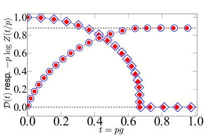
Figure 1: Death and survival probabilities. (color online) Diamonds: rescaled rate ${\cal D}(t)$ at which surviving populations die vs. scaled time $t=pg$, for two different values of $p\ll 1$, $10^{-6}(blue),$ and $10^{-7}(red)$. As $p\to 0$, the death probability converges to a limiting function that vanishes at $t=t_{e}\approx 0.67$. Circles: $-p\;\log Z(t/p)$ vs. $t$, for the same two values of $p$.

We now show how the branching ratio $U_{g}=pN_{g}$ approaches unity from below, before the IBP super-explodes. Multiplying Eq. (3) by ${\rm Prob}^{\prime}[S_{g}|N_{g}]$ and summing over $S_{g}$ gives ${\rm Prob}^{\prime}[S_{g+1}=m|N_{g}]$ conditioned on growth for $m\geq 1$ and fixed $N_{g}$. Using continuous time $t$ and changing notation, Eq. (3) leads to

$$P_{U(t)}(S,t+dt)=\sum_{S^{\prime}}P_{U(t)}(S^{\prime},t)\frac{e^{-S^{\prime}U(t)}}{1-e^{-S^{\prime}U(t)}}\frac{(S^{\prime}U(t))^{S}}{S!}.$$

Setting the conditioning variable $U(t)=U$, numerical iterations of this equation quickly converge to a stationary distribution $P_{U}(S)$ for any $U<1$. Since $U(t)$ involves an integral of $S(t)$, it has both lower fluctuations and slower variations compared to $S$, as long as $U(t)<1$. Hence, by the law of large numbers, $U(t)$ can be replaced by its mean ${\bar{U}}^{\prime}(t)$ over different realizations surviving to time $t$. Then the distribution of $S$ for a given $u\equiv{\bar{U}}^{\prime}$ is obtained from the stationary solution of

$$P_{u}(S) = \sum_{S^{\prime}}P_{u}(S^{\prime})\frac{e^{-S^{\prime}u}}{1-e^{-S^{\prime}u}}\frac{(S^{\prime}u)^{S}}{S!}.$$ (5)

Noting that as neither $p$, time, nor the age of the nodes enter Eq. (The Interacting Branching Process as a Simple Model of Innovation), we expect it to be valid for all $p\neq 0$, and also for all $\tau$ – as long as $u<1$.

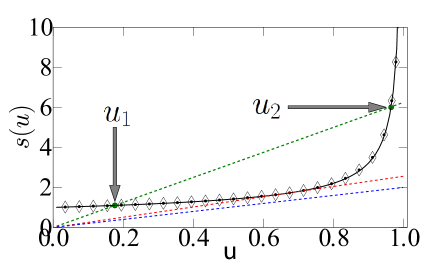
Figure 2: Mean generation size as a function of branching ratio. (color online) The solid black curve is the numerical prediction for the mean generation size $s$ vs. the mean branching ratio $u$ (both conditioned on growth) as obtained from Eq. (5). The diamonds are results of numerical simulations of the IBP. We used $p=10^{-6}$ and $\tau=\infty$, and averaged over $10^{5}$ conditioned-to-grow populations. Agreement is excellent. Also plotted are three lines showing $u/\tau$ on the y-axis, for three values of $\tau$ from top to bottom: (1) 0.16, sub-critical $\tau<\tau_{c}$, (2) critical $\tau=\tau_{c}=0.391$, and (3) 0.5, super-critical $\tau>\tau_{c}$, respectively.

We have tested the distribution given by Eq. (5) against averages over $10^{5}$ realizations of conditioned-to-grow IBP populations for small values of $p$. Fig.  2 shows our result for the mean $s\equiv{\bar{S}}^{\prime}=\sum_{S^{\prime}}S^{\prime}P_{u}(S^{\prime})$ vs. $u$. The agreement is excellent not only for the example $\tau=\infty$ shown, but also for all other $\tau>\tau_{c}\simeq 0.391$. The latter condition is explained next.

For finite $\tau$, the branching ratio evolves as $\dot{U}=S(t)-K(t)$, where $K(t)$ is the number of nodes killed at time $t$. Neglecting fluctuations gives $\dot{u}=v(u)$ where $v(u)=s(u)-u/\tau$. Fig. 2 shows that $v(u)>0$ for all $u$, if $\tau>\tau_{c}\approx 0.391$. As a result, $u(t)$ increases and eventually super-explodes, so populations have a finite probability to escape extinction.

For $\tau<\tau_{c}$, $u/\tau$ intersects $s(u)$ at two values of $u$: $u_{1}$ and $u_{2}$. The smaller of these, $u_{1}$, gives the maximal value of $u(t)$ reached before the process goes extinct. Including fluctuations in a Langevin approach, $\dot{u}=v(u)+p^{\frac{1}{2}}\omega(u)\hat{\zeta}$, with $\hat{\zeta}$ a standard Gaussian noise noise . Now the state with $u=u_{1}$ is metastable: For any finite $p$, a finite fluctuation can kick the system over the potential barrier to the unstable value $u_{2}$. Beyond $u_{2}$, $s$ is larger than $u/\tau$ for all $u$, and surviving processes again super-explode.

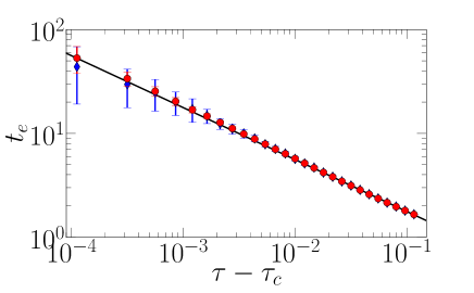
Figure 3: Mean time $\bm{t_{e}}$ to enter the super-explosive phase. (color online) The red circles (blue diamonds ) are the results of numerical simulations at $p=10^{-6}$ $(10^{-5})$ for the mean time to enter the super-explosive phase, the black curve going through them a fit $\propto(\tau-\tau_{c})^{-1/2}$.

This scenario is supported by results of numerical simulations, which we present in Fig. 3. The time, $t_{e}$, to super-explode diverges as $(\tau-\tau_{c})^{-1/2}$. It is independent of $p$, for $\tau>\tau_{c}$ provided $(\tau-\tau_{c})$ is sufficiently large. This divergence is obtained analytically by expanding $u$ about $u_{min}$ – the value where $v(u)$ reaches its minimum $v_{min}$. Writing $u=u_{min}+\epsilon$, one gets $d{\tilde{\epsilon}}/d{\tilde{t}}=1+{\tilde{\epsilon}}^{2}/2+o({\tilde{\epsilon}}^{2})$. Here, ${\tilde{\epsilon}}=\epsilon\sqrt{s_{min}^{\prime\prime}/v_{min}}$, ${\tilde{t}}=t\sqrt{s_{min}^{\prime\prime}v_{min}}$, and $s_{min}^{\prime\prime}\equiv d^{2}s/du^{2}|_{u=u_{min}}$. Surviving populations spend most of the time around $u_{min}$ before reaching $u=1$ and super-exploding. Hence, the time to explode is $t_{e}\sim(s_{min}^{\prime\prime}v_{min})^{-1/2}$. At $\tau=\tau_{c}$, $v_{min}=0$. A Taylor expansion near $\tau_{c}$ gives $v_{min}\sim\tau-\tau_{c}$, and hence $t_{e}\sim(\tau-\tau_{c})^{-1/2}$, in agreement with Fig. 3. For finite $p$, the scaling breaks down when the drift term $v_{min}$ becomes comparable to the noise, or when $v_{min}\sim(\tau-\tau_{c})\sim p^{1/2}$.

For $\tau<\tau_{c}$, the mean time to enter the explosive phase, $t_{e}$, is no longer independent of $p$ in the limit $p\rightarrow 0$. For e.g. $\tau=p$, one has $U_{g}=pS_{g}$, and $U>1$ requires $S_{g}>1/p$. The next paragraph shows that the average time to first reach $S_{g}\geq 1/p$ is $t_{e}\sim\Gamma(1/p)p^{2-(1/p)}$.

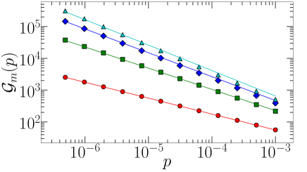
Figure 4: Mean first passage (generation) times (MFPT) to reach a generation of size ${\bm{m}}$, for $\bm{\tau=\infty}$. MFPTs for $m=2,3,4,5$ are shown from bottom to top respectively, along with the predicted values from Eq. (7). For the range of $p$ studied, numerical results obtained by averaging over $10^{6}$ surviving processes agree with predictions for $m=2,3$. For $m=4,5$ they converge to the predicted values as $p\to 0$.

Finally we estimate the mean first passage (rescaled) time, ${\cal T}_{m}(p)\equiv p{\cal G}_{m}(p)$, to a generation of size $m$ or larger in populations conditioned to reach such a generation size. We derive upper bounds by considering only the single most probable path of evolution, which become exact in the limit $p\to 0$. For any $\tau$ and small $p$, the most likely surviving process before super-exploding is a simple chain where $S_{g}=1$ for all $g$. For populations conditioned to reach $S_{g}\geq m$ for some $g$, the most likely shape is a chain up to $g-1$, and a fan-out from $S_{g-1}=1$ to $S_{g}=m$ during the last generation. All other shapes are reduced by factors of $p$. Hence for $\tau=p$ (so $U_{g^{\prime}}=p$ for all $g^{\prime}<g$ in the chain) this gives the same relative chance $p^{m-1}/m!$ to reach $S_{g}\geq m$ ( compared to $S_{g}=1$ ) at any $g$. The probability $\xi_{g}^{m}$ that $S_{g}\geq m$ has not been reached evolves as $\xi_{g+1}^{m}=\left(1-p^{m-1}/m!\right)\xi_{g}^{m}$, and thus

$${\cal G}_{m}(p)=\frac{{\cal T}_{m}(p)}{p}\sim m!\;p^{1-m}\quad({\rm for}\;\;\tau=p)\;.$$ (6)

The time $t_{e}$ can be obtained by setting $m=1/p$.

For $\tau=\infty$, $U_{g}\approx pg$ is no longer independent of $g$. The relative chance to reach $S_{g}\geq m$ ( compared to $S_{g}=1$ ) is $(pg)^{m-1}/m!$, and $\xi_{g+1}^{m}\approx(1-(pg)^{m-1}/m!)\xi_{g}^{m}$. Integrating over $g$ reveals the $g$-dependence of $\xi_{g}^{m}$, and that

$${\cal G}_{m}(p)\propto\left(\frac{1}{p}\right)^{1-1/m}\quad({\rm for}\;\;\tau=\infty)\;.$$ (7)

This is compared in Fig. 4 to direct simulations of the IBP. It describes the numerical results perfectly for $p\to 0$, and gives upper bounds for finite $p$, as it should. Eq. (7) clarifies how surviving populations evolve in the limit $p\to 0$. First, only one individual is born in each generation. Generations of size two start appearing after $p^{-1/2}$ generations, followed by the first appearance of a generation of size three after $p^{-2/3}$ generations and so on. Finally after $1/p$ generations, generations of size $s\to\infty$ appear, indicating the onset of super-explosive growth.

We have described autocatalytic networks of innovation in terms of an interacting branching process (IBP). In contrast to standard branching processes, two parents are needed to generate offspring. The IBP is both analytically and numerically tractable. In mean field theory, it shows a phase transition, which disappears due to fluctuations in a rigorous microscopic treatment. When the probability $p$ to make new innovations from any two existing ones is vanishingly small, we find universal behavior that is independent of $p$. A super-explosive phase, where the rate of new inventions grows faster than exponentially follows a long quiescent bottleneck for $p\ll 1$. This dynamics resembles the Dark Ages preceding the Renaissance or the quiescent times between bursts of speciation in punctuated biological evolution. We speculate that our models unfolds large scale properties of any co-evolutionary dynamics. Indeed its super-explosive behavior is consistent with the law of accelerating returns found in technological progress increasing ; accelerating .

References

- (1) J. Burke, Connections (Simon and Schuster, 2007).
- (2) K. Sneppen, P. Bak, H. Flyvbjerg, and M. H. Jensen, Proc. Nat. Acad. Sci. 92, 5209 (1995).
- (3) J.D. Farmer, S.A. Kauffman, and N.H. Packard, Physica D 22, 50 (1986).
- (4) R. Hanel, S. A. Kauffman, and S. Thurner, Phys. Rev. E 72, 036117 (2005).
- (5) R. Hanel, S. A. Kauffman, and S. Thurner, Phys. Rev. E 76, 036110 (2007).
- (6) H. von Foerster, P. M. Mora, L. W. Amiot, Science 132, 1291 (1960).
-
(7)
H. Moravec, Robot: mere machine to transcendent mind (Oxford University Press, 2000);
http://hoelder1in.org/Modeling_Moores_Law.html.
- (8) R. Kurzweil, The singularity is near: When humans transcend biology (Viking Adult, 2005).
- (9) B.M.E. Moret et al., IEEE Trans. Comput. Biol. 1, 13 (2004).
- (10) A. Fujikawa et al., Ethology and Sociobiol. 17, 87 (1996).
- (11) A.V. Aho and N.J.A. Sloane, Fibonacci Quarterly 11, 429 (1970).
- (12) R.D. Gray and Q.D. Atkinson, Nature 426, 435 (2003).
- (13) The noise intensity is independent of .