Abstract – We define an information topology (I-topology) and a reverse information topology (rI-topology) on the state space of a C*-subalgebra of ${\rm Mat}(n,{\mathbb{C}})$. These topologies arise from sequential convergence with respect to the relative entropy. We prove that open disks, with respect to the relative entropy, define a base for them, while Csiszár has shown in 1967 that the analogue is wrong for probability measures on a countably infinite set. The I-topology is finer than the norm topology, it disconnects the convex state space into its faces. The rI-topology is intermediate between these topologies. We complete two fundamental theorems of information geometry to the full state space, by taking the closure in the rI-topology. The norm topology is too coarse for this aim only for a non-commutative algebra, so its discrepancy to the rI-topology belongs to the quantum domain. We apply our results to the maximization of the von Neumann entropy under linear constraints and to the maximization of quantum correlations.
Index Terms – relative entropy, information topology, exponential family, convex support, Pythagorean theorem, projection theorem, maximum entropy, mutual information.
AMS Subject Classification: 81P45, 81P16, 54D55, 94A17, 90C26.

1 Introduction

Pythagorean and projection theorems in information geometry make statements about the distance of a probability measure from a family of probability measures, see e.g. Amari and Nagaoka [AN] §3 and Csiszár and Matúš [CM1] §I.C. The theorems provide a geometric frame for applications in large deviation theory or maximum-likelihood estimation. While information geometry is often confined to families of mutually absolutely continuous probability measures, some theorems have been extended [Ba, Če, CM1, CM3] using the I-/rI-convergence with respect to the relative entropy, also known as Kullback-Leibler divergence. In quantum information theory, see e.g. [AN, Be, BZ, Hi, Ho, IO, NC, Pe3], there is also a relative entropy, the Umegaki relative entropy, and one can ask the analogue questions as in classical probability theory.

An $n$-level quantum system is described by an algebra of complex $n\times n$-matrices which includes the setting of probability measures on the sample space $\{1,\ldots,n\}$ in form of the commutative algebra of diagonal matrices. It was discovered by Weis and Knauf [WK] for a $3$-level quantum system that the above theorems of information geometry can not be extended using the norm topology, because this topology is too coarse and its closures are too large. We believe that the convex geometry of a quantum state space already makes the norm topology unsuitable, which can not distinguish between the state space, a unit ball, a simplex or any other convex body. In fact, in the commutative setting, the space of probability measures on a finite measurable space is a simplex, and the norm topology does have suitable closures in order to extend e.g. maximum-likelihood estimation for exponential families, see [Ba] p. 155. On the other hand, a quantum state space is a convex body but neither a ball nor a simplex [BW]. It has a Lie group symmetry [BZ] and is studied under the name of free spectrahedron [SS] in the field of convex algebraic geometry, using techniques of algebraic geometry.

This article has two expository sections, §2 and §3, including the main ideas and results. The preparatory section §4 follows and provides techniques for subsequent analysis. The sections §5 and §6 collect the main proofs. The dependence on the matrix representation is investigated in §7.

As we shall see in section §2, the rI-topology is always first countable because the open disks of the relative entropy are its base. This is also true for the I-topology which will be discussed already in §2.1. In a sense, the I-/rI-topology combines simple properties of a metric topology with a special compatibility for geometric structure (decreasing topologies with respect to inclusion):

1. The I-topology recognizes the facial structure of the convex quantum state space, which is split into the connected components of (relative interiors of) its faces.

2. The rI-topology is adjusted to information geometry, it extends the Pythagorean and the projection theorem in topological closures.

3. The norm topology sees the state space as an arbitrary convex body.

In the setting of a non-commutative algebra of $n\times n$-matrices the I-topology is too big and the norm topology is too small to extend the Pythagorean or the projection theorem. In the commutative setting the rI-topology equals the norm topology.

In §3 we show that the rI-topology has the perfect closures to extend the Pythagorean and projection theorem to the full state space of an $n$-level quantum system. However, the extensions are proved using a combination of convex geometry and calculus of matrices, without taking the rI-topology into account.

The Pythagorean theorem implies the first solution in the literature to the maximization of the von Neumann entropy under linear constraints. This completes partial results from 1963 in Wichmann’s article [Wi]. The projection theorem has applications to quantum correlations. In §6.5 we generalize several ideas from Ay’s article [Ay] about local maximizers of correlation into the quantum setting. An essential part of our proof of the projection theorem is to study non-exposed faces of linear images of state spaces using Grünbaum’s notion of poonem [Gr]. We argue in §3.6 why poonems are needed. An analogous approach to exponential families of probability measures was taken in [CM3] with the concept of access sequence.

A broader usefulness of the I-/rI-topology in quantum statistics and quantum hypothesis testing is not yet clarified. In contrast to the commutative setting there is no canonical choice of a computational basis and the consequences for measurement and observation will have to be taken into consideration. One advance is that the infimum of the relative entropy does not decrease under information closures (21). This is useful e.g. in the Sanov theorem in quantum hypothesis testing [BS].

2 Information convergence, information topology

This is an expository section. We recall literature on information convergence and topology in §2.1 where we also define quantum state spaces and have a first discussion about topologies on the state space. After recalling some properties of the relative entropy in §2.2 we give an overview of our purely topological results for finite-level quantum systems in §2.3.

An $n$-level quantum system is described by the algebra ${\rm Mat}(n,{\mathbb{C}})$. We consider a C*-subalgebra $\mathcal{A}$ of ${\rm Mat}(n,{\mathbb{C}})$, i.e. a complex subalgebra ${\mathcal{A}}$ of ${\rm Mat}(n,{\mathbb{C}})$ closed under the adjoint map $a\mapsto a^{*}$. The definition of a C*-subalgebra includes completeness with respect to a norm, but this is clear in finite dimensions. We prefer the term C*-subalgebra because it reminds us of the complex field ${\mathbb{C}}$ and of the closure under the adjoint map. Unless otherwise stated, ${\mathcal{A}}$ is a C*-subalgebra of ${\rm Mat}(n,{\mathbb{C}})$.

2.1 Spaces of probability measures and quantum states

We discuss convergence with respect to the relative entropy, called information convergence. For finite measurable spaces we discuss the associated topology in detail. Then we generalize to finite-level quantum systems and we finish with a short discussion of infinite-dimensional commutative von Neumann algebras. All proofs and further issues follow in §5. A review of information convergence and its topology in probability theory is given in §I.C in [CM1].

Let $\mathcal{M}$ be a set of probability measures on a measurable space $(X,\mathcal{X})$. If $P,Q\in\mathcal{M}$ are absolutely continuous with respect to a $\sigma$-finite measure $\lambda$ and $p(x)$ resp. $q(x)$ is the Radon-Nikodym derivative of $P$ resp. $Q$, then the relative entropy is

$$\textstyle D(P||Q)\;:=\;\int_{X}p(x)\log\tfrac{p(x)}{q(x)}d\lambda\,.$$ (1)

This equals zero if and only if $P=Q$ and otherwise $D(P||Q)$ is strictly positive or $+\infty$, see [KL]. The total variation is

$$\textstyle\|P-Q\|_{1}\;:=\;\int_{X}|p(x)-q(x)|d\lambda\,.$$ (2)

It is well-known that total variation defines a norm on the space of signed measures having a density with respect to $\lambda$. The Pinsker-Csiszár inequality [Gi] shows

$$\textstyle\|P-Q\|_{1}^{2}\;\leq\;2D(P||Q)\,.$$ (3)

Given a sequence $(P_{k})_{k\in\mathbb{N}}\subset\mathcal{M}$ and a probability measure $P\in\mathcal{M}$ we have, according to [CM1], I-convergence resp. rI-convergence of $(P_{k})_{k\in\mathbb{N}}$ to $P$ if

$$\textstyle\lim_{k\to\infty}D(P_{k}||P)\;=\;0\qquad\text{resp.}\qquad\lim_{k\to\infty}D(P||P_{k})\;=\;0\,.$$ (4)

Csiszár has studied these convergences in the context of the $f$-divergence, generalizing the relative entropy. He has proved in Theorem 3 in [Cs2] that the information neighborhoods, defined for $P\in\mathcal{M}$ and $\epsilon>0$ by

$$\textstyle\{Q\in\mathcal{M}\mid D(Q||P)<\epsilon\}\qquad\text{resp.}\qquad\{Q\in\mathcal{M}\mid D(P||Q)<\epsilon\}\,,$$ (5)

are not a base of a topology if $(X,\mathcal{X})=({\mathbb{N}},2^{\mathbb{N}})$ where $2^{\mathbb{N}}$ is the power set of ${\mathbb{N}}$.

In spite of Csiszár’s negative result it is possible to define an I-topology resp. rI-topology on ${\mathcal{M}}$ in terms of the convergence of (countable) sequences (4), see Dudley and Harremoës [Du2, Hs]. Here a subset $U\subset{\mathcal{M}}$ is open if for each probability measure $P\in U$ and each sequence $(P_{k})_{k\in\mathbb{N}}\subset\mathcal{M}$ that I- resp. rI-converges to $P$, there exists $N\in{\mathbb{N}}$ such that for all $k\geq N$ we have $P_{k}\in U$. It follows from (3) that the I-/rI-topology is finer than the norm topology of the total variation.

We will take the approach by Dudley and Harremoës to study information topologies for an $n$-level quantum system. The common ground between finite-level quantum systems and spaces of probability measures are spaces of probability measures on a finite measurable space. The probability simplex of a non-empty (at most) countable set $X$ is

$$\textstyle{\mathbb{P}}(X)\;:=\;\{p=(p_{x})_{x\in X}\in[0,1]^{X}\mid\sum_{x\in X}p_{x}=1\}\,.$$ (6)

Elements $p$ of ${\mathbb{P}}(X)$ are called probability vectors on $X$ and can be identified with probability measures $P$ on $(X,2^{X})$ using $P(A):=\sum_{x\in A}p_{x}$ for $A\subset X$. For a finite measurable space $X=\{1,\ldots,n\}$ the probability simplex ${\mathbb{P}}(X)$ is a simplex of dimension $n-1$ and the information neighborhoods (5) are a base of a topology. The rI-topology on ${\mathbb{P}}(X)$ equals the total variation topology, which is the restriction of the standard Euclidean topology on ${\mathbb{R}}^{X}$. The I-topology splits ${\mathbb{P}}(X)$ into connected components $C(X^{\prime})$ of constant support $X^{\prime}\subset X$,

$$\textstyle C(X^{\prime})\;:=\;\{p\in{\mathbb{P}}(X)\mid p_{x}>0\iff x\in X^{\prime}\}\,.$$

On each connected component the I-topology equals the norm topology. This decomposition into connected components is the stratification (44) of the probability simplex into relative interiors of its faces.

To describe the I-/rI-topology for a C*-subalgebra $\mathcal{A}$ of ${\rm Mat}(n,{\mathbb{C}})$ let us introduce some notation. We denote the identity in ${\rm Mat}(n,{\mathbb{C}})$ by $\mathds{1}_{n}$ (the zero by $0_{n}$ or $0$) and the identity in ${\mathcal{A}}$ by $\mathds{1}$. A state on ${\mathcal{A}}$ is a complex linear functional $f:{\mathcal{A}}\to{\mathbb{C}}$, such that $f(a^{*}a)\geq 0$ for all $a\in{\mathcal{A}}$ and $f(\mathds{1})=1$. The standard trace $\operatorname{tr}$ turns ${\rm Mat}(n,{\mathbb{C}})$ into a complex Hilbert space with the Hilbert-Schmidt inner product $\langle a,b\rangle\,:=\,\operatorname{tr}(ab^{*})$ for $a,b\in{\rm Mat}(n,{\mathbb{C}})$ and we use the two-norm $\|a\|_{2}:=\sqrt{\langle a,a\rangle}$. By ${\mathcal{A}}_{\rm sa}$ we denote the real vector space of self-adjoint matrices in ${\mathcal{A}}$ and $({\mathcal{A}}_{\rm sa},\langle\cdot,\cdot\rangle)$ is a Euclidean vector space. We call its norm topology on any subset simply norm topology as all norms are equivalent in finite dimensions.

There is a one-to-one correspondence between states $f$ on ${\mathcal{A}}$ and matrices in ${\mathcal{A}}$ which are positive semi-definite ($\rho\succeq 0$) and have trace one ($\operatorname{tr}(\rho)=1$), see e.g. Theorem 2.4.21 in [BR]. The functional $f$ and the matrix $\rho$ are related by

$$\textstyle f(a)\;=\;\langle a,\rho\rangle\qquad(a\in{\mathcal{A}})\,.$$ (7)

The matrix representation $\rho$ of $f$ is called density matrix in quantum mechanics. We will use the terms of state and density matrix synonymously. The state space is

$$\textstyle{\mathcal{S}}\;=\;{\mathcal{S}}_{\mathcal{A}}\;:=\;\{\rho\in{\mathcal{A}}\mid\rho\succeq 0,\operatorname{tr}(\rho)=1\,\}\,.$$ (8)

For the commutative subalgebra ${\mathcal{A}}$ of complex diagonal matrices of size $n\times n$ the state space is the probability simplex (6),

$$\textstyle{\mathbb{P}}(\{1,\ldots,n\})\;=\;{\mathcal{S}}_{\mathcal{A}}\;\subset\;{\rm Mat}(n,{\mathbb{C}})\,.$$ (9)

We will show for a possibly non-commutative C*-subalgebra $\mathcal{A}$ of ${\rm Mat}(n,{\mathbb{C}})$ that the analogues of information neighborhoods (5) are bases of two topologies. For a non-commutative algebra ${\mathcal{A}}$ the analogue of the rI-topology is strictly finer than the norm topology (Corollary 5.19) and it defines—unlike the norm topology—useful closures in information theory, as we shall outline in §3.

We show in Theorem 5.18.3 that the analogue of the I-topology splits ${\mathcal{S}}$ into connected components of states $\rho\in\mathcal{S}$ of constant support $s(\rho)\in{\mathcal{A}}$. Here we use the partial ordering $\preceq$ on ${\mathcal{A}}$ defined by $a\preceq b$ for $a,b\in{\mathcal{A}}$ if and only if $b-a$ is positive semi-definite. The projection lattice ${\mathcal{P}}$ of the algebra ${\mathcal{A}}$ is

$$\textstyle{\mathcal{P}}\;=\;{\mathcal{P}}_{\mathcal{A}}\;:=\;\{p\in{\mathcal{A}}\mid p^{2}=p^{*}=p\}\,,$$ (10)

its elements are projections. The partial ordering restricts to ${\mathcal{P}}$, more details about lattices are discussed in §4.1 and infinite-dimensional algebras are treated e.g. in [AS]. The support projection of a self-adjoint matrix $a\in{\mathcal{A}}$ is the infimum

$$\textstyle s(a)\;:=\;\bigwedge\{p\in{\mathcal{P}}\mid pa=a\}\,.$$

Again, like for the probability simplex ${\mathbb{P}}(X)$, the decomposition of ${\mathcal{S}}$ into connected components is the stratification (44) of the state space ${\mathcal{S}}$ into relative interiors of its faces. Of course, ${\mathcal{S}}$ is homeomorphic in the norm topology to the closed Euclidean unit ball. This is a property of any convex body, i.e. compact and convex subset of Euclidean space, known as the Theorem of Sz. Nagy, see e.g. §VIII.1 in [Br].

In the algebraic formalism, the measurable space $({\mathbb{N}},2^{\mathbb{N}})$ corresponds to the von Neumann algebra of bounded sequences

$$\textstyle l^{\infty}\;:=\;\{x=(x_{i})_{i\in{\mathbb{N}}}\in{\mathbb{C}}^{\mathbb{N}}\mid\sup_{i\in{\mathbb{N}}}|x_{i}|<\infty\}$$

acting by multiplication on the Hilbert space $l^{2}:=\{x\in l^{\infty}\mid\sum_{i\in{\mathbb{N}}}|x_{i}|^{2}<\infty\}$ of square summable sequences. The space $l^{1}:=\{x\in l^{\infty}\mid\sum_{i\in{\mathbb{N}}}|x_{i}|<\infty\}$ of absolutely summable sequences contains the probability simplex ${\mathbb{P}}({\mathbb{N}})$. This has, for the algebra ${\mathcal{A}}=l^{\infty}$, the form (8) of a state space if we denote for $x\in l^{1}$ the set of inequalities $x_{i}\geq 0$ for all $i\in{\mathbb{N}}$ simultaneously by $x\succeq 0$ and if we use the trace ${\rm tr}:l^{1}\to{\mathbb{C}}$, $x\mapsto\sum_{i\in{\mathbb{N}}}x_{i}$,

$$\textstyle{\mathbb{P}}({\mathbb{N}})\;=\;{\mathcal{S}}_{\mathcal{A}}\;=\;\{x\in l^{1}\mid x\succeq 0,{\rm tr}(x)=1\}\,.$$

The discussion above shows that the information neighborhoods (5) do not define a topology on ${\mathbb{P}}({\mathbb{N}})$ but two topologies are defined in terms of the convergences (4).

2.2 The relative entropy

The relative entropy is a measure of distance between states. It has an operational meaning e.g. in hypothesis testing [Pe3]. We recall well-known convexity and continuity properties. Although the relative entropy is not continuous in the norm topology, we point out that it is continuous in the I-topology in its first argument and continuous in the rI-topology in its second argument (17).

Definition 2.1.

The relative entropy of a density matrix $\rho\in{\mathcal{S}}$ from $\sigma\in{\mathcal{S}}$ is

$$\textstyle S(\rho,\sigma)\;:=\;\operatorname{tr}\rho(\log(\rho)-\log(\sigma))$$ (11)

if ${\rm Im}(\rho)\subset{\rm Im}(\sigma)$. Otherwise $S(\rho,\sigma):=+\infty$. The logarithm can be defined by functional calculus, see Remark 4.23.3.

The relative entropy (11) satisfies $S(\rho,\sigma)\geq 0$ for all $\rho,\sigma\in{\mathcal{S}}$ with equality if and only if $\rho=\sigma$, see e.g. §11.3 in [Pe3] or §11.3 of [NC]. It is discontinuous (in the norm topology) in the first argument already for the algebra ${\mathcal{A}}={\mathbb{C}}^{2}$ of a bit and in the second argument for the algebra ${\mathcal{A}}={\rm Mat}(2,{\mathbb{C}})$ of a qubit.

Example 2.2.

If ${\mathcal{A}}={\mathbb{C}}^{2}$ then $S\left((\tfrac{n-1}{n},\tfrac{1}{n}),(1,0)\right)=\infty$ for all $n\in{\mathbb{N}}$ while $S\left((1,0),(1,0)\right)=0$. If ${\mathcal{A}}={\rm Mat}(2,{\mathbb{C}})$, then for real $\alpha$ we have

$$\textstyle S\left(\tfrac{1}{2}(\mathds{1}_{2}+\sigma_{1}),\tfrac{1}{2}(\mathds{1}_{2}+\cos(\alpha)\sigma_{1}+\sin(\alpha)\sigma_{2})\right)\;=\;\left\{\begin{array}[]{rl}0&\text{if }\alpha=0\mod 2\pi,\\ \infty&\text{else.}\end{array}\right.$$

Example 11 in [WK] is less trivial: A smooth curve $t\mapsto\sigma_{t}$ converging in norm to $\rho$ on the boundary of the Bloch ball ${\mathcal{S}}_{{\rm Mat}(2,{\mathbb{C}})}$ can have any non-negative limit of $S(\rho,\sigma_{t})$.

Let us now turn to some well-known properties of the relative entropy.

Definition 2.3.

1. A function $f:X\to(-\infty,\infty]$, defined on a convex subset $X$ of a finite-dimensional Euclidean vector space ${\mathbb{E}}$, is convex if for $x_{1},x_{2}\in X$ and $\lambda\in[0,1]$

   $$\textstyle f((1-\lambda)x_{1}+\lambda x_{2})\;\leq\;(1-\lambda)f(x_{1})+\lambda f(x_{2})\,.$$

   In the special case that $Y$ is another convex subset of ${\mathbb{E}}$ and $f:X\times Y\to(-\infty,\infty]$ is defined, such that for $x_{1},x_{2}\in X$, $y_{1},y_{2}\in Y$ and $\lambda\in[0,1]$ we have

   $$\textstyle f((1-\lambda)x_{1}+\lambda x_{2},(1-\lambda)y_{1}+\lambda y_{2})\;\leq\;(1-\lambda)f(x_{1},y_{1})+\lambda f(x_{2},y_{2})$$

   then $f$ is called jointly convex. A function $f:X\to{\mathbb{R}}$ is strictly convex if for $x,y\in X$, $x\neq y$ and $\lambda\in(0,1)$

   $$\textstyle f((1-\lambda)x+\lambda y)\;<\;(1-\lambda)f(x)+\lambda f(y)\,.$$

   If $f$ is (strictly) convex, we say that $-f$ is (strictly) concave.

2. If $(X,d)$ is a metric space and $f:X\to(-\infty,\infty]$ then $f$ is lower semi-continuous if for all $x\in X$ and every sequence $(x_{i})_{i\in\mathbb{N}}\subset X$ converging to $x$ we have

   $$\textstyle\liminf_{i\to\infty}f(x_{i})\;\geq\;f(x)\,.$$

Remark 2.4.

1. The lower semi-continuity of the relative entropy (in the norm topology) is proved e.g. by Wehrl in §III.B in [We], using Lindblad’s representation of the relative entropy [Ld]. Ohya and Petz give another proof in §5 in [OP]. They use Kosaki’s formula and write the relative entropy as a supremum of affine functionals.

2. The joint convexity of the relative entropy follows from Lieb’s theorem [Li], see e.g. §11.4 in [NC] or §III in [We] for proofs and the historic context. Convexity of the relative entropy is a special case of the joint convexity of quasi-entropies [Pe1]. Also, it follows easily from the monotonicity of the relative entropy under quantum operations, see §3.4 in [Pe3].

3. A convex lower semi-continuous function is continuous along straight lines. More precisely, let $f:X\to(-\infty,\infty]$ be a convex and lower semi-continuous function defined on a closed convex subset $X$ of a finite-dimensional Euclidean vector space ${\mathbb{E}}$. We extend $f$ to ${\mathbb{E}}$ by setting its value to $+\infty$ outside of $X$. Since $X$ is convex, the extension $\widetilde{f}$ is convex. Since $X$ is closed, $\widetilde{f}$ is lower semi-continuous. Thus, Corollary 7.5.1 in [Ro] shows for $x,y\in{\mathbb{E}}$, subject to $\widetilde{f}(x)<+\infty$, that

   $$\textstyle\widetilde{f}(y)\;=\;\lim_{\lambda\nearrow 1}\widetilde{f}((1-\lambda)x+\lambda y)\,.$$

   Here the values of $\widetilde{f}$ converge in the Alexandroff compactification $(-\infty,\infty]$ of ${\mathbb{R}}$, see Example 5.12. For example, if $\tau\in{\mathcal{S}}$ is any invertible density matrix, then for arbitrary $\rho,\sigma\in{\mathcal{S}}$ we have $S(\rho,\tau)<\infty$ so

   $$\textstyle S(\rho,\sigma)\;=\;\lim_{\lambda\nearrow 1}S(\rho,(1-\lambda)\tau+\lambda\sigma)\,.$$ (12)

   We use (12) in Theorem 5.18.5 to prove that the state space ${\mathcal{S}}$ is connected in the rI-topology.

2.3 New results about the I- and the rI-topology

This section summarizes properties of the I-/rI-topology of a C*-subalgebra ${\mathcal{A}}$ of ${\rm Mat}(n,{\mathbb{C}})$ with focus on similarities to a metric topology. Reasoning is done within the theory of sequential convergence, recalled in §5, exceptions are the Pinsker-Csiszár inequality (15) and the continuity result of (17) which are from matrix theory. Since the I-topology and the rI-topology share many properties, we use a prefix variable $\omega\in\{{\rm I},{\rm rI}\}$ to denote

$$\omega \omega$$-topology, -closure, etc.

Unless otherwise specified we always use the norm topology. We end the section with an application in information theory.

Definition 2.5 (Information topology).

1. We use short-hand notation for the two possible variable orderings of the relative entropy (11),

   $$\textstyle S^{\rm I}(\rho,\sigma)\;:=\;S(\sigma,\rho)\qquad\text{and}\qquad S^{\rm rI}(\rho,\sigma)\;:=\;S(\rho,\sigma)\,.$$

   If $\{A(i)\}_{i\in{\mathbb{N}}}$ is a sequence of statements, then we shall say that $A(i)$ is true for large $i$ if there is $N\in{\mathbb{N}}$ such that $A(i)$ holds for all $i\geq N$. We define a family of subsets of the state space ${\mathcal{S}}$ by

   $$\textstyle{\mathcal{T}}^{\omega}\;:=\;\left\{U\subset{\mathcal{S}}\;\mid\begin{array}[]{l}\text{if }\rho\in U,(\rho_{i})_{i\in{\mathbb{N}}}\subset{\mathcal{S}}\text{ and }\lim_{i\to\infty}S^{\omega}(\rho,\rho_{i})=0\,,\\ \text{then }\rho_{i}\in U\text{ for large }i\end{array}\right\}\,.$$

   The open $\omega$-disk about $\rho\in{\mathcal{S}}$ with radius $\epsilon\in(0,\infty]$ is

   $$\textstyle V^{\omega}(\rho,\epsilon)\;:=\;\{\sigma\in{\mathcal{S}}\mid S^{\omega}(\rho,\sigma)<\epsilon\}$$ (13)

   and the closed $\omega$-disk about $\rho\in{\mathcal{S}}$ with radius $\epsilon\in(0,\infty]$ is

   $$\textstyle W^{\omega}(\rho,\epsilon)\;:=\;\{\sigma\in{\mathcal{S}}\mid S^{\omega}(\rho,\sigma)\leq\epsilon\}\,.$$ (14)

   We denote the (unique) norm topology on ${\mathcal{S}}$ by ${\mathcal{T}}^{\|\cdot\|}$. For $a\in{\mathcal{A}}$ and $(a_{i})_{i\in{\mathbb{N}}}\subset{\mathcal{A}}$ we denote by $\lim_{i\to\infty}a_{i}=a$ the convergence of $(a_{i})_{i\in{\mathbb{N}}}$ to $a$ in norm.

2. Let $(X,\mathcal{T})$ be a topological space. The topology $\mathcal{T}$ is a Hausdorff topology if each two distinct points of $X$ belong to two disjoint open sets. A family $\mathcal{B}\subset\mathcal{T}$ is a base for $(X,\mathcal{T})$ if any non-empty open subset of $X$ is a union of a subfamily of $\mathcal{B}$. A family $\mathcal{B}(x)$ of open sets containing $x\in X$ is called a base for $(X,\mathcal{T})$ at $x$ if for any open set $V$ containing $x$ there exists $U\in\mathcal{B}(x)$ such that $U\subset V$. The topological space $(X,\mathcal{T})$ is first-countable if there exists a countable base at every point $x\in X$, it is second-countable if it has a countable base.

The family ${\mathcal{T}}^{\omega}$ is easily seen to be a topology on ${\mathcal{S}}$, which we call the $\omega$-topology. The inclusion ${\mathcal{T}}^{\|\cdot\|}\subset{\mathcal{T}}^{\omega}$ follows directly from the Pinsker-Csiszár inequality, which confirms for $\rho,\sigma\in{\mathcal{S}}$ that

$$\textstyle\|\rho-\sigma\|_{1}^{2}\;\leq\;2S(\rho,\sigma)\,.$$ (15)

Here the trace norm from Definition 4.1.2 is used, see e.g. §3.4 in [Pe3] for a proof. The inclusion ${\mathcal{T}}^{\|\cdot\|}\subset{\mathcal{T}}^{\omega}$ implies that the $\omega$-topology is a Hausdorff topology. The convergence of sequences a priori, in terms of the relative entropy, is equivalent to the convergence a posteriori, in terms of the $\omega$-topology. This is formalized as the equivalence a) below, which in Theorem 5.18 takes the form of $C({\mathcal{T}}^{\omega})=C^{\omega}$. For sequences $(\rho_{i})_{i\in{\mathbb{N}}}\subset{\mathcal{S}}$ and states $\rho\in{\mathcal{S}}$ we have

$$\textstyle\lim_{i\to\infty}S^{\omega}(\rho,\rho_{i})=0\;\stackrel{{\scriptstyle\textup{a)}}}{{\iff}}\; \textstyle\forall U\in{\mathcal{T}}^{\omega}\text{ with }\rho\in U\text{ we have }\rho_{i}\in U\text{ for large }i$$ (16)

$$\textstyle\;\stackrel{{\scriptstyle\textup{b)}}}{{\iff}}\; \textstyle\forall\epsilon\in(0,\infty]\text{ we have }\rho_{i}\in V^{\omega}(\rho,\epsilon)\text{ for large }i\,.$$

Equivalence a) holds more generally for any divergence function in the sense of §5.1. In particular, a) holds for infinite-dimensional algebras.

The equivalence b) is more restrictive. It follows from a continuity property. In Proposition 5.16 we use (15), and for the case $\omega={\rm rI}$ some perturbation theory, to show for all $\rho,\sigma\in{\mathcal{S}}$ and $(\sigma_{i})_{i\in{\mathbb{N}}}\subset{\mathcal{S}}$

$$\textstyle\lim_{i\to\infty}S^{\omega}(\sigma,\sigma_{i})\;=\;0\quad\implies\quad\lim_{i\to\infty}S^{\omega}(\rho,\sigma_{i})\;=\;S^{\omega}(\rho,\sigma)\,.$$ (17)

In Theorem 5.18.2 we show that (17) means that the relative entropy is continuous in the first argument for the I-topology and in the second argument for the rI-topology. Therefore the open $\omega$-disks are a base of ${\mathcal{T}}^{\omega}$, which is equivalent to b) in (16). Hence ${\mathcal{T}}^{\omega}$ is first-countable while Corollary 5.19 shows that ${\mathcal{T}}^{\omega}$ is second-countable if and only if $\mathcal{A}$ is commutative. The continuity (17) is wrong for the infinite-dimensional algebra $l^{\infty}$, where the open $\omega$-disks are not a base of a topology, see §2.1.

In addition to proving distance-like properties (16), we use (17) in Theorem 5.18.4 to show

$$\textstyle{\mathcal{T}}^{\|\cdot\|}\;\subset\;{\mathcal{T}}^{\rm rI}\;\subset\;{\mathcal{T}}^{\rm I}\,.$$ (18)

Equivalently we have for all sequences $(\rho_{i})_{i\in{\mathbb{N}}}\subset{\mathcal{S}}$ and states $\rho\in{\mathcal{S}}$ the ordering of convergences

$$\textstyle\lim_{i\to\infty}S(\rho_{i},\rho)\;=\;0\quad\implies\quad\lim_{i\to\infty}S(\rho,\rho_{i})\;=\;0\quad\implies\quad\lim_{i\to\infty}\rho_{i}\;=\;\rho\,.$$

Later in Corollary 5.19 we prove the proper inclusion ${\mathcal{T}}^{\|\cdot\|}\subsetneq{\mathcal{T}}^{\rm rI}$ for non-commutative algebras, whereas ${\mathcal{T}}^{\rm rI}\subsetneq{\mathcal{T}}^{\rm I}$ holds already for the algebra ${\mathbb{C}}^{2}$ of a bit. Other conditions for commutativity will be mentioned in §6.6.

The infimum of the relative entropy between a state and a set of states is useful in information theory and in quantum information theory, e.g. to compute optimal error rates in hypothesis testing [BS].

Definition 2.6 ($\omega$-closure).

For $\rho\in{\mathcal{S}}$ and $X\subset{\mathcal{S}}$ we write

$$\textstyle S^{\omega}(\rho,X)\;:=\;\inf_{\tau\in X}S^{\omega}(\rho,\tau)$$ (19)

and we define the $\omega$-closure of $X\subset{\mathcal{S}}$ by

$$\textstyle{\rm cl}^{\omega}(X)\;:=\;\{\rho\in{\mathcal{S}}\mid S^{\omega}(\rho,X)=0\}\,.$$ (20)

In a C*-subalgebra of ${\rm Mat}(n,{\mathbb{C}})$ we can show in Theorem 5.18.2 for an arbitrary subset $X\subset{\mathcal{S}}$ of states that the $\omega$-closure ${\rm cl}^{\omega}(X)$ is the topological closure of $X$ with respect to ${\mathcal{T}}^{\omega}$. Differently frased, we have for all $\rho\in{\mathcal{S}}$

$$\textstyle S^{\omega}(\rho,{\rm cl}^{\omega}(X))\;=\;S^{\omega}(\rho,X)\,.$$ (21)

This is also proved in Corollary 5.17 directly from (17). The analogue statement for spaces of probability measures on infinite $\sigma$-algebras is wrong by Example 5.4.

3 New results about exponential families

This is an expository section about exponential families in a C*-subalgebra ${\mathcal{A}}$ of ${\rm Mat}(n,{\mathbb{C}})$. With the exception of some corollaries, all proofs are done in §6. We begin in §3.1 by explaining and proving the Pythagorean theorem and the projection theorem in a restriction where this is easy. In §3.2 and §3.3 we define an extension of every exponential family, by lifting faces of a convex parameter space. In §3.4 we explain a new Pythagorean theorem, valid for this extension. A corollary solves the problem of maximizing the von Neumann entropy under linear constraints. This is the first complete solution in the literature. In §3.5 we explain a new projection theorem, valid for the extension. A corollary shows that the extension is the rI-closure of the exponential family.

The Staffelberg family [WK] in §3.5 shows that the norm topology is too coarse to extend an exponential family appropriately, its closures are too large. The Swallow family [WK] in §3.6 demonstrates why poonems [Gr] are essential in our proof of the projection theorem.

Issues proved in §6 but not covered in the present section include applications to quantum correlations in §6.5 and equality conditions for closures of exponential families in §6.6.

3.1 A recap of elementary information geometry

We recall the Pythagorean theorem and the projection theorem for the relative entropy in a C*-subalgebra ${\mathcal{A}}$ of ${\rm Mat}(n,{\mathbb{C}})$. The aim of this article is to extended them from the invertible states to the whole state space. These theorems are exemplary for many elegant ideas in information geometry [Am1]. The following Pythagorean theorem has first appeared in articles [Pe2, Na] by Petz and Nagaoka. It is well-known [Na, AN, Je] that it fits into the differential-geometric context of dually flat spaces, initiated by Amari [Am1].

The Pythagorean theorem of relative entropy applies to states $\rho,\sigma,\tau\in{\mathcal{S}}$ where $\sigma,\tau$ are invertible and $\rho-\sigma$ is orthogonal to $\log(\tau)-\log(\sigma)$ with respect to the Hilbert-Schmidt inner product. An elementary calculation shows for the relative entropy $S$

$$\textstyle S(\rho,\sigma)\,+\,S(\sigma,\tau)\;=\;S(\rho,\tau)\,.$$ (22)

With relative entropy (11) replaced by squared Euclidean distance, this equation reminds us of the Pythagorean theorem in Euclidean geometry. See also §3.4 in [Pe3] and §3.4 in [AN] for further information, as well as §7 in [AN] for an overview of applications in estimation theory.

Definition 3.1.

We use the real analytic function $R_{\mathcal{A}}:{\mathcal{A}}_{\rm sa}\to{\mathcal{A}}_{\rm sa}$,

$$\textstyle R(\theta)\;=\;R_{\mathcal{A}}(\theta)\;:=\;\exp_{\mathcal{A}}(\theta)/\operatorname{tr}(\exp_{\mathcal{A}}(\theta))\,.$$ (23)

The exponential $\exp_{\mathcal{A}}$ is defined by functional calculus in the algebra ${\mathcal{A}}$, see Definition 4.22.3 and Remark 4.23.2. For a non-empty real affine subspace $\Theta\subset{\mathcal{A}}_{\rm sa}$ we define an exponential family in ${\mathcal{A}}$ by

$$\textstyle{\mathcal{E}}\;:=\;R_{\mathcal{A}}(\Theta)\;=\;\{R_{\mathcal{A}}(\theta)\mid\theta\in\Theta\,\}\,.$$ (24)

The parametrization $R_{\mathcal{A}}$ is the canonical parametrization of ${\mathcal{E}}$. We call a one-dimensional exponential family (with/-out parametrization) e-geodesic. We use the translation vector space $U:=\operatorname{lin}(\Theta)=\Theta-\Theta=\{\theta_{1}-\theta_{2}\mid\theta_{1},\theta_{2}\in\Theta\}$.

We mention vocabulary in the literature. The analogue of the parametrization $R_{\mathcal{A}}$ of an exponential family is called canonical parametrization in probability theory, see §20 in [Če]. For an affine map $a:{\mathbb{R}}\to\Theta$ the curve $\gamma:t\mapsto R_{\mathcal{A}}\circ a(t)$ is called e-geodesic in §3.4 in [Pe3]. This curve is called $(+1)$-geodesic in Section 7.2 in [AN] while an e-geodesic is a more general concept there, see also Remark 4 in [WK].

Figure 1: The Staffelberg family is sketched by e-geodesics (thin curves). The Euclidean geodesic from $\sigma$ to $\rho$ meets the e-geodesic from $\sigma$ to $\tau$ (red) orthogonally with respect to the BKM-metric: The Pythagorean theorem $S(\rho,\sigma)+S(\sigma,\tau)=S(\rho,\tau)$ holds. Closure components in different topologies are indicated (bold).

Example 3.2 (The Staffelberg family).

We shall use Pauli $\sigma$-matrices $\sigma_{1}:=\left(\begin{smallmatrix}0&1\\ 1&0\end{smallmatrix}\right)$, $\sigma_{2}:=\left(\begin{smallmatrix}0&-i\\ i&0\end{smallmatrix}\right)$ and $\sigma_{3}:=\left(\begin{smallmatrix}1&0\\ 0&-1\end{smallmatrix}\right)$. The Staffelberg family, studied in [WK], is the exponential family

$$\textstyle R({\rm span}_{\mathbb{R}}(\sigma_{1}\oplus 0,\,\sigma_{2}\oplus 1\,))\;\subset\;{\rm Mat}(2,{\mathbb{C}})\oplus{\mathbb{C}}\;\cong\;\left(\begin{smallmatrix}*&*&0\\ {}*&*&0\\ 0&0&*\end{smallmatrix}\right)\;\subset\;{\rm Mat}(3,{\mathbb{C}})$$

embedded into ${\rm Mat}(3,{\mathbb{C}})$ by block diagonal matrices. The Staffelberg family is depicted in Figure 1. The pointed circle about the family is an equator of the Bloch ball ${\mathcal{S}}({\rm Mat}(2,{\mathbb{C}}))$, parametrized for real $\alpha$ by $\rho(\alpha):=\tfrac{1}{2}(\mathds{1}_{2}+\sin(\alpha)\sigma_{1}+\cos(\alpha)\sigma_{2})\oplus 0$. The figure also shows $c:=\tfrac{1}{2}(\rho(0)+0_{2}\oplus 1)$. Figure 4 shows the Staffelberg family inside the state space ${\mathcal{S}}_{\mathcal{B}}:=\{\rho\in{\mathcal{B}}\mid\rho\succeq 0,{\rm tr}(\rho)=1\}$ of the real *-subalgebra ${\mathcal{B}}$ spanned by $\sigma_{1}\oplus 0$, $\sigma_{2}\oplus 0$, ${\rm i}\sigma_{3}\oplus 0$, ${\rm diag}(1,1,0)$ and $\mathds{1}_{3}$. The algebra ${\mathcal{B}}$ is closed under real scalar multiplication and under the adjoint map. Its state space is a 3D cone with apex $0_{2}\oplus 1$ based on the circle $\{\rho(\alpha)\mid\alpha\in{\mathbb{R}}\}$.

The Pythagorean theorem (22) applies to exponential families. For states $\rho\in{\mathcal{S}}$ and $\sigma,\tau\in{\mathcal{E}}$, such that $\rho-\sigma$ is perpendicular to the translation vector space $U$, with respect to the Hilbert-Schmidt scalar product, we have

$$\textstyle S(\rho,\sigma)+S(\sigma,\tau)=S(\rho,\tau)\,.$$ (25)

The condition $\rho-\sigma\perp U$ means that the Euclidean straight line from $\sigma$ to $\rho$ is perpendicular to the exponential family ${\mathcal{E}}$ with respect to the BKM-Riemannian metric, see Remark 6.2. This is indicated by the right angle in Figure 1.

The projection theorem, is now an easy corollary. For every state $\rho\in{\mathcal{E}}+U^{\perp}$ the intersection $(\rho+U^{\perp})\cap{\mathcal{E}}$ contains a unique state $\pi_{\mathcal{E}}(\rho)$, which defines a projection to ${\mathcal{E}}$

$$\pi_{\mathcal{E}}:\;({\mathcal{E}}+U^{\perp})\cap{\mathcal{S}}\;\to\;{\mathcal{E}}\,,\quad\rho\;\mapsto\;\pi_{\mathcal{E}}(\rho)\,.$$ (26)

By the choice of $\rho$ the intersection is non-empty. If it contains two states $\sigma,\tau$, then $\rho-\sigma\perp U$ and $\rho-\tau\perp U$. Equality $\sigma=\tau$ follows if we add the two corresponding Pythagorean equations (25). The minimal relative entropy of $\rho$ from $\mathcal{E}$, called entropy distance in [WK], is

$$\textstyle{\rm d}_{\mathcal{E}}(\rho)\;:=\;\inf_{\tau\in{\mathcal{E}}}S(\rho,\tau)\,.$$ (27)

If $\rho\in{\mathcal{E}}+U^{\perp}$ then (25) implies the projection theorem

$$\textstyle{\rm d}_{\mathcal{E}}(\rho)\;=\;S(\rho,\pi_{\mathcal{E}}(\rho))\,.$$ (28)

A geometric optimization formula like (28) is called a projection theorem in §3.4 in [AN]. We will extend (28) in this article to arbitrary states $\rho$.

3.2 An algorithm for poonems of the mean value set

We use two equivalent descriptions of the convex set of mean values. Its boundary components are described algebraically in a lattice ${\mathcal{P}}^{U}$ of projections.

Definition 3.3.

The mean value set of a linear subspace $U\subset{\mathcal{A}}_{\rm sa}$ of self-adjoint matrices is the orthogonal projection of the state space onto $U$

$$\textstyle{\mathbb{M}}(U)\;=\;{\mathbb{M}}_{\mathcal{A}}(U)\;:=\;\pi_{U}({\mathcal{S}}_{\mathcal{A}})\;\subset\;U\,.$$ (29)

Here $\pi_{U}:{\mathcal{A}}_{\rm sa}\to U$ denotes the orthogonal projection from ${\mathcal{A}}_{\rm sa}$ onto $U$. This linear mapping is characterized for each $a\in{\mathcal{A}}_{\rm sa}$ by the equation $a-\pi_{U}(a)\perp U$. For $u_{1},\ldots,u_{k}\in{\mathcal{A}}_{\rm sa}$ we abbreviate ${\bf u}:=(u_{1},\ldots,u_{k})$ and we define the mean value mapping by

$$\textstyle m_{\bf u}:\;{\mathcal{A}}_{\rm sa}\;\to\;{\mathbb{R}}^{k}\,,\quad a\;\mapsto\;(\langle u_{1},a\rangle,\ldots,\langle u_{k},a\rangle)\,.$$ (30)

The convex support of ${\bf u}$ is

$$\textstyle{\rm cs}({\bf u})\;=\;{\rm cs}_{\mathcal{A}}({\bf u})\;:=\;\{m_{\bf u}(\rho)\mid\rho\in{\mathcal{S}}_{\mathcal{A}}\}\;\subset\;{\mathbb{R}}^{k}\,.$$ (31)

The concept of convex support was first used by Barndorff-Nielsen [Ba] in probability theory and later by Čencov [Če]. It was refined by Csiszár and Matúš [CM1, CM3] to investigate mean values of exponential families. Barndorff-Nielsen’s definition for a finite measurable space is equivalent to (31) if probability measures are embedded into an algebra of diagonal matrices like in (9).

The convex support introduces coordinates on the mean value set ${\mathbb{M}}(U)$. If $U:={\rm span}_{\mathbb{R}}(u_{1},\ldots,u_{k})$, then the convex bodies ${\mathbb{M}}(U)\cong{\rm cs}({\bf u})$ are “affinely isomorphic” (see Remark 1.1.1 in [We3]): The mean value mapping restricts to the bijection

$$\textstyle m_{\bf u}|_{{\mathbb{M}}(U)}:\;{\mathbb{M}}(U)\;\to\;{\rm cs}({\bf u})$$ (32)

such that $m_{\bf u}\circ\pi_{U}=m_{\bf u}$. In the majority of all proofs we are going to use the Hilbert-Schmidt Euclidean geometry in ${\mathcal{A}}_{\rm sa}$, using orthogonal projection $\pi_{U}$ rather than coordinates.

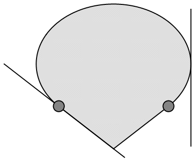
Figure 2: This clove shape is the mean value set of the Swallow family. It is the convex hull of an ellipse and a point (Example 3.4). The supporting hyperplane to the left resp. right defines an exposed face which is a segment resp. a point. Two non-exposed faces (points) of the clove are indicated by small disks.

The simplest boundary component of a convex set $C$ in Euclidean space is an exposed face of $C$, the set of maximizers in $C$ of a linear functional. The empty set is an exposed face by definition. Except for $\emptyset$ and $C$, every exposed face of $C$ is the intersection of $C$ and a supporting hyperplane $H$, i.e. an affine subspace $H$ of codimension one which intersects $C$ such that $C\setminus H$ is convex. Figure 2 shows examples.

Figure 3: Repeated inclusions of exposed faces define a poonem. Here a poonem of point form is visualized by the disk .

A poonem [Gr] of $C$ is a member of a sequence $F_{1}\subset\cdots\subset F_{k}=C$, s.th. $F_{i}$ is an exposed face of $F_{i+1}$ for $i=1,\ldots,k-1$. A non-exposed face of $C$ is a poonem of $C$, which is not an exposed face of $C$. Figure 3 shows an example of a poonem, which is a non-exposed face. The notion of poonem is equivalent to the notion of face (see e.g. §1.2.1 in [We2] for a proof) which we will use in §4.1. The set of exposed faces and the set of poonems are partially ordered by inclusion, they are lattices.

The first step to the extension of ${\mathcal{E}}$ is a lifting construction for poonems of the mean value set ${\mathbb{M}}(U)$. For every poonem $P$ of ${\mathbb{M}}(U)$ the inverse image under projection $\{\rho\in{\mathcal{S}}\mid\pi_{U}(\rho)\in P\}$ is an exposed face of the state space ${\mathcal{S}}$. For every exposed face $F$ of the state space ${\mathcal{S}}$ there exists a unique projection $p\in{\mathcal{P}}_{\mathcal{A}}$ in the projection lattice (10) of ${\mathcal{A}}$, such that

$$\textstyle F\;=\;{\mathcal{S}}_{p{\mathcal{A}}p}\;=\;\{\rho\in p{\mathcal{A}}p\mid\rho\succeq 0,{\rm tr}(\rho)=1\}\,.$$

The C*-subalgebra $p{\mathcal{A}}p=\{pap\mid a\in{\mathcal{A}}\}$ is called compressed algebra. Let us collect in the projection lattice

$$\textstyle{\mathcal{P}}^{U}$$ (33)

all the projections arising in this construction from poonems of ${\mathbb{M}}(U)$. The projection lattice ${\mathcal{P}}^{U}$ ordered by $\preceq$ is isomorphic to the lattice of poonems of ${\mathbb{M}}(U)$ ordered by inclusion. An algorithm to compute ${\mathcal{P}}^{U}$ is described in Remark 4.17. This is the algebraic reformulation of the concept of poonem for the special case of a mean value set.

3.3 The extension of an exponential family

We introduce an extension to the exponential family defined in (23) in terms of a non-empty affine subspace $\Theta\subset{\mathcal{A}}_{\rm sa}$ of self-adjoint matrices,

$$\textstyle{\mathcal{E}}\;=\;R_{\mathcal{A}}(\Theta)\;=\;\{\exp_{\mathcal{A}}(\theta)/{\rm tr}\exp_{\mathcal{A}}(\theta)\mid\theta\in\Theta\}\,.$$

The translation vector space of $\Theta$ is $U:=\Theta-\Theta$. To each poonem of the mean value set ${\mathbb{M}}(U)$ corresponds a projection $p\in{\mathcal{P}}^{U}$, we associate an exponential family to $p$ and take the union over all $p\in{\mathcal{P}}^{U}$.

Figure 4: The Staffelberg family (left) and Swallow family (right) are sketched by e-geodesics inside the conic state space (real algebra). The boundary of the mean value set (projection of the state space) is drawn underneath each family.

Example 3.4.

The Swallow family, studied in [WK], is the exponential family

$$\textstyle R({\rm span}_{\mathbb{R}}(\sigma_{1}\oplus 1,\,\sigma_{2}\oplus 1\,))\,.$$

Figure 4 shows two exponential families ${\mathcal{E}}$ inside the conic state space ${\mathcal{S}}_{\mathcal{B}}$ of the real algebra ${\mathcal{B}}$ from Example 3.2. The figure also shows the mean value sets ${\mathbb{M}}(V)$, translated into the drawing frame, with respect to the canonical tangent space [WK]

$$\textstyle V\;:=\;\{\log(\rho)-{\rm tr}(\log(\rho))\mathds{1}_{3}/3\mid\rho\in{\mathcal{E}}\}\,.$$

The projection of the 3D cone ${\mathcal{S}}_{\mathcal{B}}$ onto $V$ equals the mean value set ${\mathbb{M}}_{\mathcal{A}}(V)$ for algebras ${\mathcal{A}}={\rm Mat}(3,{\mathbb{C}})$ or ${\mathcal{A}}={\rm Mat}(2,{\mathbb{C}})\oplus{\mathbb{C}}$. This follows from Theorem 6.5 as $\mathcal{E}$ is included in the state space ${\mathcal{S}}_{\mathcal{B}}$. This also follows from simpler arguments about state spaces, see Lemma 3.13 in [We3]. So ${\mathbb{M}}(V)=\pi_{V}({\mathcal{S}}_{\mathcal{B}})$ is the convex hull of an ellipse and a point.

We now consider an affine space $p\Theta p=\{p\theta p\mid\theta\in\Theta\}$ for each $p\in{\mathcal{P}}^{U}$ and we use it to define an exponential family in the compressed algebra $p{\mathcal{A}}p$ by

$$\textstyle{\mathcal{E}}_{p}\;:=\;R_{p{\mathcal{A}}p}(p\Theta p)\;=\;\{p\exp(p\theta p)/{\rm tr}(p\exp(p\theta p))\mid\theta\in\Theta\}$$ (34)

using the normalized exponential $R_{p{\mathcal{A}}p}$ in (23). Noticing $\mathds{1}\in{\mathcal{P}}^{U}$ and ${\mathcal{E}}_{\mathds{1}}={\mathcal{E}}$, the disjoint union

$$\textstyle{\rm ext}({\mathcal{E}})\;:=\;\bigcup_{p\in{\mathcal{P}}^{U}\setminus\{0\}}{\mathcal{E}}_{p}$$ (35)

contains ${\mathcal{E}}$ and we will prove in Lemma 6.9 a bijection between this extension and the mean value set

$$\textstyle\pi_{U}|_{{\rm ext}({\mathcal{E}})}:\;{\rm ext}({\mathcal{E}})\;\to\;{\mathbb{M}}(U)\,.$$ (36)

This allows us to define a projection

$$\textstyle\pi_{\mathcal{E}}:\;{\mathcal{S}}\;\to\;{\rm ext}({\mathcal{E}})\,,$$ (37)

such that $\pi_{U}(\rho)=\pi_{U}\circ\pi_{\mathcal{E}}(\rho)$ holds for all states $\rho$.

The bijection (36) is based on the lattice analysis outlined above and on the mean value chart of exponential families, proved in [Wi] and generalized in §6.1.

Example 3.5 (Extension).

The Staffelberg family, shown in Figure 1, is extended by the pointed circle $\{\rho(\alpha)\mid\alpha\in(0,2\pi)\}$ of one-point exponential families, the states $\rho(\alpha)$ being defined in Example 3.2, and by $c=\tfrac{1}{2}(0_{2}\oplus 1+\rho(0))$. Their union is in one-to-one correspondence with the elliptical boundary of the mean value set. Figure 4 shows the Staffelberg family with its mean value set. It also shows the Swallow family, where the extension contains two one-dimensional exponential families, the open segments between $0_{2}\oplus 1$ and $\rho(0)$ resp. $\rho(\tfrac{\pi}{2})$. The extension of the Swallow family is the norm closure. The extension of the Staffelberg family is strictly smaller than the norm closure.

The projection lattice ${\mathcal{P}}^{V}$ of these exponential families ${\mathcal{E}}$ is computed in §3.3 in [We3]. The rI-closure ${\rm cl}^{\rm rI}({\mathcal{E}})$ is computed in §IV.B and §IV.D in [WK]. By Theorem 6.16 the rI-closure ${\rm cl}^{\rm rI}({\mathcal{E}})$ is the extension ${\rm ext}({\mathcal{E}})$ which is computed directly from the projection lattice ${\mathcal{P}}^{V}$ in [WK].

3.4 The Complete Pythagorean theorem

We will extend in Theorem 6.12 the Pythagorean theorem (25) to the full state space using the extension previously defined. A corollary is the maximization of the von Neumann entropy under linear constraints, a fundamental problem in quantum statistical mechanics, see e.g. [IO, Ru, Pe3, AN].

Theorem (Complete Pythagorean theorem).

For any $\rho\in{\mathcal{S}}$ and $\sigma,\tau\in{\rm ext}({\mathcal{E}})$ such that $\rho-\sigma\perp U$ we have $S(\rho,\sigma)+S(\sigma,\tau)=S(\rho,\tau)$.

Definition 3.6.

The von Neumann entropy of $\rho\in{\mathcal{S}}$ is defined by

$$\textstyle S(\rho)\;:=\;-\operatorname{tr}\rho\log(\rho)\,,$$ (38)

using functional calculus, see Remark 4.23.3. The free energy of $\theta\in{\mathcal{A}}_{\rm sa}$ is

$$\textstyle F(\theta)\;=\;F_{\mathcal{A}}(\theta)\;:=\;\log\operatorname{tr}\exp_{\mathcal{A}}(\theta)\,,$$ (39)

where $\exp_{\mathcal{A}}$ is defined by functional calculus in ${\mathcal{A}}$, see (23).

According to Jaynes [Ja] the state which maximizes the von Neumann entropy under arbitrary constraints is the least biased choice of a state compatible with the constraints. Exponential families with linear canonical parameter space $\Theta=U$ are called Gibbsian families [Pe3], they maximize the von Neumann entropy under linear constraints. We can show this for their extension, too. Let $u_{1},\ldots,u_{k}\in{\mathcal{A}}_{\rm sa}$, put $\Theta:=U:={\rm span}_{\mathbb{R}}(u_{1},\ldots,u_{k})$, ${\mathcal{E}}:=R_{\mathcal{A}}(U)$ and denote ${\bf u}=(u_{1},\ldots,u_{k})$. We consider the mean value map $m_{\bf u}$ and the convex support ${\rm cs}({\bf u})=m_{\bf u}({\mathcal{S}})$, defined respectively in (30) and (31).

Corollary 3.7.

For all $x\in{\rm cs}({\bf u})$ there exists a unique state $\sigma\in{\rm ext}({\mathcal{E}})$ such that $\sigma={\rm argmax}\{S(\rho)\mid\rho\in{\mathcal{S}},m_{\bf u}(\rho)=x\}$.

Proof: Using the bijections (36) and (32) there exists a unique state $\sigma\in{\rm ext}({\mathcal{E}})$ such that $m_{\bf u}(\sigma)=x$. Let $\rho\in{\mathcal{S}}$ such that $m_{\bf u}(\rho)=m_{\bf u}(\sigma)=x$. Then by (32) we have $\rho-\sigma\perp U$. Using $S(\rho)=\log({\rm tr}\,\mathds{1})-S(\rho,\tfrac{1}{{\rm tr}\,\mathds{1}}\mathds{1})$, the Complete Pythagorean theorem, applied to the states $\rho,\sigma$ and $\tau:=\tfrac{1}{{\rm tr}\,\mathds{1}}\mathds{1}\in{\mathcal{E}}$, shows

$$\textstyle S(\sigma)-S(\rho)\;=\;S(\rho,\tau)-S(\sigma,\tau)\;=\;S(\rho,\sigma)\,.$$

The claim follows from the distance-like properties of the relative entropy, see §2.2. $\Box$

There exist coordinates $\beta_{1},\ldots,\beta_{k}$ for a Gibbsian family ${\mathcal{E}}$ analogous to inverse temperatures in statistical mechanics [IO]—this explains the sign convention of $-\beta$ (not $+\beta$) below. The extension ${\rm ext}({\mathcal{E}})$ has a second parameter specifying the support projection. We consider the projection lattice ${\mathcal{P}}^{U}$ and the free energy $F$, defined respectively in (33) and (39).

Corollary 3.8.

For every mean value tuple $x=(\xi_{1},\dots,\xi_{k})\in{\rm cs}_{\mathcal{A}}({\bf u})$ there is a unique maximizer $\rho(x)$ of the von Neumann entropy among all states $\rho\in{\mathcal{S}}_{\mathcal{A}}$ with mean values $m_{\bf u}(\rho)=x$. There exists a unique projection $p\in{\mathcal{P}}^{U}\setminus\{0\}$ and there exist (generally not unique) numbers $\beta_{1},\ldots,\beta_{k}\in{\mathbb{R}}$, such that

$$\textstyle\tfrac{\partial}{\partial\beta_{j}}\,F_{p{\mathcal{A}}p}(-\sum_{i=1}^{k}\beta_{i}pu_{i}p)\;=\;-\xi_{j}\,,\qquad j=1,\ldots,k\,.$$

For each solution $p,\beta_{1},\ldots,\beta_{k}$ we have

$$\textstyle\rho(x)\;=\;R_{p{\mathcal{A}}p}(-\sum_{i=1}^{k}\beta_{i}pu_{i}p)$$

and $\rho(x)$ has the von Neumann entropy $S(\rho(x))=\sum_{i=1}^{k}\beta_{i}\xi_{i}+F_{p{\mathcal{A}}p}(-\sum_{i=1}^{k}\beta_{i}pu_{i}p)$.

Proof: Corollary 3.7 shows that the extension ${\rm ext}({\mathcal{E}})$ is the set of unique maximizers of the von Neumann entropy under the linear constraints. Corollary 6.11 provides the described coordinates. It remains to compute the von Neumann entropy of $\rho:=\rho(x)=R_{p{\mathcal{A}}p}(p(-\sum_{i=1}^{k}\beta_{i}u_{i})p)$. By definition of $R_{p{\mathcal{A}}p}$ in (23) we have

$$S(\rho) \;=\;-{\rm tr}\rho\log(\rho)$$

$$\;=\;{\textstyle-\operatorname{tr}\rho[-\sum_{i=1}^{k}\beta_{i}pu_{i}p-F_{p{\mathcal{A}}p}(-\sum_{i=1}^{k}\beta_{i}pu_{i}p)]}$$

$$\;=\;{\textstyle\sum_{i=1}^{k}\beta_{i}\langle pu_{i}p,\rho\rangle+F_{p{\mathcal{A}}p}(-\sum_{i=1}^{k}\beta_{i}pu_{i}p)}\,.$$

We have $\langle pu_{i}p,\rho\rangle=\langle u_{i},\rho\rangle=\xi_{i}$ for $i=1,\ldots,k$ because $\rho$ has support $s(\rho)=p$. $\Box$

In the paragraph following Corollary 6.11 we comment on the uniqueness of parameters $\beta_{1},\ldots,\beta_{k}$. The special case of Corollary 3.8 for states of full support $s(\rho)=\mathds{1}$ in ${\mathcal{A}}$ was known already in 1963. To explain it, let ${\rm ri}(C)$ denote the relative interior of a convex subset $C$ in Euclidean space, i.e. ${\rm ri}(C)$ is the interior of $C$ in the norm topology of the affine hull of $C$. Wichmann [Wi] has proved the bijection

$$\textstyle\pi_{U}|_{\mathcal{E}}:\;{\mathcal{E}}\;\to\;{\rm ri}\,{\mathbb{M}}(U)\,.$$ (40)

It implies the Pythagorean theorem (25) and the projection theorem (28) for all states $\rho\in U+{\rm ri}\,{\mathbb{M}}(U)$, in particular for all invertible states $\rho$. This holds since $\pi_{U}({\rm ri}\,{\mathcal{S}})={\rm ri}\,{\mathbb{M}}(U)$ and because the relative interior ${\rm ri}\,{\mathcal{S}}$ consists of the invertible states, see e.g. Proposition 4.5. The map

$$\textstyle\Phi:\;{\rm cs}({\bf u})\;\to\;{\mathcal{S}}\,,\quad x\;\mapsto\;{\rm argmax}\{S(\rho)\mid\rho\in{\mathcal{S}},m_{\bf u}(\rho)=x\}$$ (41)

parametrizes ${\rm ext}({\mathcal{E}})$ by mean values. Wichmann has shown the following:

1. $\Phi({\rm ri}\,{\rm cs}({\bf u}))={\mathcal{E}}$,

2. $\Phi|_{{\rm ri}\,{\rm cs}({\bf u})}:$ ${\rm ri}\,{\rm cs}({\bf u})\to{\mathcal{E}}$ is real analytic,

3. $\Phi({\rm cs}({\bf u}))\subset\overline{{\mathcal{E}}}$, where $\overline{{\mathcal{E}}}$ denotes the closure of ${\mathcal{E}}$ in the norm topology.

Our result of $\Phi({\rm cs}({\bf u}))={\rm ext}({\mathcal{E}})$ in Corollary 3.8 resolves $\Phi({\rm cs}({\bf u}))\subset\overline{{\mathcal{E}}}$ to an equality. However we do not know how tight the upper bound $\Phi({\rm cs}({\bf u}))\subset\overline{{\mathcal{E}}}$ is. This question is related to the continuity of $\Phi$. A discontinuous $\Phi$ is presented in Example 3.10, see also Proposition 6.22.

3.5 The Complete projection theorem

The following theorem and its corollary hold for our standard assumptions of an affine space $\Theta$ and ${\mathcal{E}}=R_{\mathcal{A}}(\Theta)$. We extend in Theorem 6.16 the projection theorem (28) to the full state space using the extension ${\rm ext}({\mathcal{E}})$ previously defined. As a corollary we write ${\rm ext}({\mathcal{E}})$ as the topological closure in the rI-topology.

For technical reasons we write $S_{\rho}(\sigma):=S(\rho,\sigma)$ for the relative entropy with fixed state $\rho$ and variable state $\sigma$. We use the entropy distance

$$\textstyle{\rm d}_{\mathcal{E}}(\rho)\;=\;\inf_{\sigma\in{\mathcal{E}}}S_{\rho}(\sigma)$$

and the projection $\pi_{\mathcal{E}}$ defined in (27) and (37) respectively.

Theorem (Complete projection theorem).

For each $\rho\in{\mathcal{S}}$ the relative entropy $S_{\rho}$ has on the extension ${\rm ext}({\mathcal{E}})$ a unique local minimizer at $\pi_{\mathcal{E}}(\rho)$. We have

$$\textstyle{\rm d}_{\mathcal{E}}(\rho)\;=\;\min_{\sigma\in{\rm ext}({\mathcal{E}})}S_{\rho}(\sigma)\;=\;S_{\rho}(\pi_{\mathcal{E}}(\rho))\,.$$

The Complete projection theorem shows ${\rm ext}({\mathcal{E}})=\{\rho\in{\mathcal{S}}\mid{\rm d}_{\mathcal{E}}(\rho)=0\}$, where the right-hand side is the rI-closure ${\rm cl}^{\rm rI}({\mathcal{E}})$ of ${\mathcal{E}}$ defined in (20). Theorem 5.18.2 shows that ${\rm cl}^{\rm rI}({\mathcal{E}})$ is the topological closure of ${\mathcal{E}}$ with respect to the rI-topology. This topology can be defined by the base $\{V^{\rm rI}(\rho,\epsilon)\mid\epsilon\in(0,\infty]\}$ of open rI-disks $V^{\rm rI}(\rho,\epsilon)=\{\sigma\in{\mathcal{S}}\mid S(\rho,\sigma)<\epsilon\}$. To sum up:

Corollary 3.9.

We have ${\rm ext}({\mathcal{E}})={\rm cl}^{\rm rI}({\mathcal{E}})$.

We have seen in (18) that the rI-topology is finer than the norm topology. So ${\rm cl}^{\rm rI}({\mathcal{E}})\subset\overline{{\mathcal{E}}}$ is obvious. A proper inclusion is possible.

Example 3.10.

The Staffelberg family ${\mathcal{E}}$ from Example 3.2 satisfies ${\rm cl}^{\rm rI}(\mathcal{E})\subsetneq\overline{\mathcal{E}}$. This exponential family is depicted in Figure 1: The norm closure $\overline{\mathcal{E}}$ is the union of $\mathcal{E}$ with the bold circle around $\mathcal{E}$ and the dashed upright segment from $\rho(0)$ to $0_{2}\oplus 1$. The upright segment is missing in the rI-closure ${\rm cl}^{\rm rI}(\mathcal{E})$ except for its top endpoint $c$. See §IV.B in [WK] for this analysis.

The Staffelberg is a Gibbsian family (with $\tfrac{1}{{\rm tr}\mathds{1}}\mathds{1}\in{\mathcal{E}}$). The rI-closure ${\rm cl}^{\rm rI}({\mathcal{E}})$ is a set of maximizers of the von Neumann entropy under linear constraints. The norm closure $\overline{{\mathcal{E}}}$ is too large for this aim.

3.6 Why poonems are essential

Poonems are essential for the Complete projection theorem. Strictly speaking, the bijection in Lemma 6.9

$$\textstyle\pi_{U}|_{{\rm ext}({\mathcal{E}})}:\;{\rm ext}({\mathcal{E}})\;\to\;{\mathbb{M}}(U)$$

as well as the Complete Pythagorean theorem can be proved without any need for poonems—using the equivalent notion of face.

The first reason to use poonems is that the algebraic algorithm in Remark 4.17 to compute the projection lattice ${\mathcal{P}}^{U}$ proceeds along chains of faces of ${\mathbb{M}}(U)$

$$\textstyle{\mathbb{M}}(U)\;=\;F_{0}\;\supsetneq\;F_{1}\;\supsetneq\;\cdots\;\supsetneq\;F_{m}$$ (42)

such that $F_{i+1}$ is an exposed face of $F_{i}$ for $i=0,\ldots,m-1$. Elements of such chains are poonems by definition. Though the projection lattice ${\mathcal{P}}^{U}$ is essential for defining the extension ${\rm ext}({\mathcal{E}})$ in (35) we are not forced to use the algorithm, since ${\mathcal{P}}^{U}$ is defined in (46) in terms of lattice isomorphisms.

Chains (42) and the algorithm are essential in the Complete projection theorem. Certainly, if $\rho$ is a state, $p\in{\mathcal{P}}^{U}$ and $\pi_{U}(\rho)\in\pi_{U}({\mathcal{E}}_{p})$ then we can compute the minimum

$$\textstyle{\rm d}_{{\mathcal{E}}_{p}}(\rho)\;=\;\inf\{S_{\rho}(\sigma)\mid\sigma\in{\mathcal{E}}_{p}\}\,.$$

This will be done in Proposition 6.15 in the paragraph following (80). But it is not clear how the value ${\rm d}_{{\mathcal{E}}_{p}}(\rho)$ is related to ${\rm d}_{{\mathcal{E}}_{q}}(\rho)$ for $q\succeq p$, $q\in{\mathcal{P}}^{U}$. The equality ${\rm d}_{{\mathcal{E}}_{p}}(\rho)={\rm d}_{{\mathcal{E}}_{q}}(\rho)$ will be proved by approximation of ${\mathcal{E}}_{p}$ from within ${\mathcal{E}}_{q}$, using e-geodesics. E-geodesics guarantee a controlled limit of the (discontinuous) relative entropy (Lemma 6.14). It is not possible to exhaust the extension ${\rm ext}({\mathcal{E}})$ in one step of such an approximation. In fact, we show in Proposition 6.21 that the union $X$ of an exponential family ${\mathcal{E}}$ with the two limit points of all in ${\mathcal{E}}$ included e-geodesics covers only part of the mean value set ${\mathbb{M}}(U)$ under the projection $\pi_{U}$. Relative interiors of non-exposed faces of ${\mathbb{M}}(U)$ are missing.

The Swallow family ${\mathcal{E}}=R_{{\mathcal{A}}}(V)$ in Example 3.4 makes this clear. Two non-exposed faces of the mean value set ${\mathbb{M}}(V)$ are depicted in Figure 2. As depicted in Figure 4, each of these non-exposed faces has a unique inverse projection under $\pi_{U}$, which is $\rho(\alpha)$ for $\alpha\in\{0,\tfrac{\pi}{2}\}$. So there exists no e-geodesic in ${\mathcal{E}}$ with limit $\rho(\alpha)$ although $\rho(\alpha)$ belongs to the extension ${\rm ext}({\mathcal{E}})$ and a fortiori to the norm closure $\overline{{\mathcal{E}}}$. On the other hand, the open segment between $0_{2}\oplus 1$ and $\rho(\alpha)$ is included in $X$ and it is an exponential family ${\mathcal{E}}_{p}$, corresponding to the rank-two projection $p=\rho(\alpha)+0_{2}\oplus 1\in{\mathcal{P}}^{V}$. Now $\rho(\alpha)$ can be approximated in a second step by the e-geodesic ${\mathcal{E}}_{p}$. The corresponding faces of the mean value set ${\mathbb{M}}(V)$ are

$$\textstyle\pi_{V}({\mathcal{S}})={\mathbb{M}}(V)\quad\supsetneq\quad\pi_{V}(\text{segment between }0_{2}\oplus 1\text{ and }\rho(\alpha))\quad\supsetneq\quad\pi_{V}(\rho(\alpha))\,.$$

They are depicted schematically in Figure 3 and they form a chain (42).

For details about missing e-geodesic limits at non-exposed faces we refer to the proof of Proposition 6.21. For explicit calculations on the Swallow family we refer to Remark 29 a) in [WK].

4 Analysis on the state space

This a preparatory section summarizing techniques from convex geometry, geometry of state spaces and mean value sets including their algebraic formulation. Detailed perturbation theoretical proofs are provided in §4.3, where the standard theory is not sufficient.

Let us introduce important notations. The use of spectral values may seem unnecessary. We have decided to work with the extension ${\rm ext}({\mathcal{E}})=\bigcup_{p\in{\mathcal{P}}^{U}\setminus\{0\}}{\mathcal{E}}_{p}$ of an exponential family (35) as a single object in the Euclidean space ${\mathcal{A}}_{\rm sa}$. Thus we need to distinguish between invertibility in several compressed algebras $p{\mathcal{A}}p$.

Definition 4.1 (Spectral values, norms and Euclidean vector spaces).

1. Let $a\in{\mathcal{A}}$. The spectrum of $a$ is

   $$\textstyle{\rm spec}_{\mathcal{A}}(a):=\{\lambda\in{\mathbb{C}}\mid a-\lambda\mathds{1}\text{ is not invertible in }{\mathcal{A}}\},$$

   its elements are the spectral values of $a$ in ${\mathcal{A}}$. The matrix $a$ is positive semi-definite if $a\in{\mathcal{A}}_{\rm sa}$ and if $a$ has no negative spectral values, we then write $a\succeq 0$. If $a\succeq 0$, then there exists $b\in{\mathcal{A}}$, $b\succeq 0$ with $a=b^{2}$, see e.g. §2.2 in [Mu]. The matrix $b$ is unique and one defines $\sqrt{a}:=b$. We have $a^{*}a\succeq 0$ and put $|a|:=\sqrt{a^{*}a}$.

2. In addition to the two-norm $\|\cdot\|_{2}$ introduced in §2.1 we consider the spectral norm $\|a\|$, which is the square root of the largest eigenvalue of $a^{*}a$ and the trace norm $\|a\|_{1}:=\operatorname{tr}|a|$. The topology of any norm is the norm topology and convergence of a sequence $(a_{i})_{i\in{\mathbb{N}}}\subset{\mathcal{A}}$ to $a\in{\mathcal{A}}$ in any norm will be denoted by $\lim_{i\to\infty}a_{i}=a$. The three norms restrict to the real vector space of self-adjoint matrices ${\mathcal{A}}_{\rm sa}$.

3. In any Euclidean vector space $({\mathbb{E}},\langle\cdot,\cdot\rangle)$ we denote the two-norm by $\|x\|_{2}:=\sqrt{\langle x,x\rangle}$ and write $x\perp y:\iff\langle x,y\rangle=0$ for $x,y\in{\mathbb{E}}$. For subsets $X,Y\subset{\mathbb{E}}$ we write $X\perp Y:\iff\langle x,y\rangle=0\,\forall x\in X,y\in Y$ and $X^{\perp}:=\{y\in{\mathbb{E}}\mid x\perp y\,\forall x\in X\}$ (if $z\in{\mathbb{E}}$ then $z\perp Y:\iff\{z\}\perp Y$ and $z^{\perp}:=\{z\}^{\perp}$). If ${\mathbb{A}}$ is a non-empty affine subspace of ${\mathbb{E}}$, then we denote the translation vector space of ${\mathbb{A}}$ by

   $$\textstyle\operatorname{lin}({\mathbb{A}})\;:=\;{\mathbb{A}}-{\mathbb{A}}\;=\;\{a-b\mid a,b\in{\mathbb{A}}\}\,.$$

   We denote the orthogonal projection from ${\mathbb{E}}$ onto ${\mathbb{A}}$ by $\pi_{\mathbb{A}}:{\mathbb{E}}\to{\mathbb{A}}$. This affine mapping is characterized for each $x\in{\mathbb{E}}$ by the equation $x-\pi_{\mathbb{A}}(x)\perp\operatorname{lin}({\mathbb{A}})$.

4.1 Lattices of faces and projections

In this section we settle the convex geometry and the algebraic description of the mean value set ${\mathbb{M}}(U)=\pi_{U}({\mathcal{S}})$, referring to [We2, We3]. The mean value set (29) is the orthogonal projection of the state space ${\mathcal{S}}$ onto a linear subspace $U\subset{\mathcal{A}}_{\rm sa}$. Notice that [We3] erroneously uses eigenvalues and not spectral values. The corrected statements are cited below from the copy on the arXiv.

A map $f:X\to Y$ between two partially ordered sets $(X,\leq)$ and $(Y,\leq)$ is isotone if for all $x,y\in X$ such that $x\leq y$ we have $f(x)\leq f(y)$. A lattice is a partially ordered set $({\mathcal{L}},\leq)$ where the infimum $x\wedge y$ and supremum $x\vee y$ of each two elements $x,y\in{\mathcal{L}}$ exist. A lattice isomorphism is a bijection between two lattices that preserves the lattice structure. A lattice ${\mathcal{L}}$ is complete if for an arbitrary subset $S\subset{\mathcal{L}}$ the infimum $\bigwedge S$ and the supremum $\bigvee S$ exist. The least element $\bigwedge{\mathcal{L}}$ and the greatest element $\bigvee{\mathcal{L}}$ in a complete lattice ${\mathcal{L}}$ are improper elements of ${\mathcal{L}}$, all other elements of ${\mathcal{L}}$ are proper elements. An atom of a complete lattice ${\mathcal{L}}$ is an element $x\in{\mathcal{L}}$, $x\neq\bigwedge{\mathcal{L}}$, such that $y\leq x$ and $y\neq x$ implies $y=\bigwedge{\mathcal{L}}$ for all $y\in{\mathcal{L}}$.

The projection lattice ${\mathcal{P}}=\{p\in{\mathcal{A}}\mid p^{2}=p^{*}=p\}$, defined in (10), with the partial ordering $\preceq$ is a complete lattice. For this and the following two statements see e.g. [AS] or Remark 2.6 in [We3]. For a self-adjoint (also normal) matrix $a\in{\mathcal{A}}_{\rm sa}$ we have

$$\textstyle a\;=\;pap\quad\iff\quad pa\;=\;a\quad\iff\quad s(a)\;\preceq\;p\,.$$ (43)

Hence the partial ordering for projections $p,q\in{\mathcal{P}}$ simplifies to $p\preceq q\iff pq=p$.

We need two distinct notions of “ face ” of a convex set, each defining a lattice of subsets ordered by inclusion. We begin with a general convex set.

Definition 4.2.

Let $({\mathbb{E}},\langle\cdot,\cdot\rangle)$ be a finite-dimensional Euclidean vector space.

1. The closed segment between $x,y\in{\mathbb{E}}$ is $[x,y]:=\{(1-\lambda)x+\lambda y\mid\lambda\in[0,1]\}$, the open segment is $]x,y[\,:=\{(1-\lambda)x+\lambda y\mid\lambda\in(0,1)\}$. A subset $C\subset{\mathbb{E}}$ is convex if $x,y\in C$ $\implies$ $[x,y]\subset C$.

2. Let $C$ be a convex subset of ${\mathbb{E}}$. A face of $C$ is a convex subset $F$ of $C$, such that whenever for $x,y\in C$ the open segment $]x,y[$ intersects $F$, then the closed segment $[x,y]$ is included in $F$. If $x\in C$ and $\{x\}$ is a face, then $x$ is called an extreme point. The set of faces of $C$ will be denoted by ${\mathcal{F}}(C)$, called the face lattice of $C$.

3. The support function of a convex subset $C\subset{\mathbb{E}}$ is defined by ${\mathbb{E}}\to{\mathbb{R}}\cup\{\pm\infty\}$, $u\mapsto h(C,u):=\sup_{x\in C}\langle u,x\rangle$. For non-zero $u\in{\mathbb{E}}$ the set

   $$H(C,u)\;:=\;\{x\in{\mathbb{E}}:\langle u,x\rangle=h(C,u)\}$$

   is an affine hyperplane unless it is empty, which can happen if $C=\emptyset$ or if $C$ is unbounded in $u$-direction. If $C\cap H(C,u)\neq\emptyset$, then we call $H(C,u)$ a supporting hyperplane of $C$. The exposed face of $C$ by $u$ is

   $$F_{\perp}(C,u)\;:=\;C\cap H(C,u)$$

   and we put $F_{\perp}(C,0):=C$. The faces $\emptyset$ and $C$ are exposed faces of $C$ by definition. The set of exposed faces of $C$ will be denoted by ${\mathcal{F}}_{\perp}(C)$, called the exposed face lattice of $C$. A face of $C$, which is not an exposed face is a non-exposed face and we then say the face $F$ is not exposed.

4. Some topology is needed. Let $X\subset{\mathbb{E}}$ be an arbitrary subset. The affine hull of $X$, denoted by $\operatorname{aff}(X)$, is the smallest affine subspace of ${\mathbb{E}}$ that contains $X$. The interior of $X$ with respect to the relative topology of $\operatorname{aff}(X)$ is the relative interior $\operatorname{ri}(X)$ of $X$. The complement $\operatorname{rb}(X):=X\setminus\operatorname{ri}(X)$ is the relative boundary of $X$. If $C\subset{\mathbb{E}}$ is a non-empty convex subset then we consider the vector space $\operatorname{lin}(C)=\{x-y\mid x,y\in\operatorname{aff}(C)\}$. We define the dimension $\dim(C):=\dim(\operatorname{lin}(C))$ and $\dim(\emptyset):=-1$.

Remark 4.3.

1. As observed e.g. in [WK, We2], the mean value set ${\mathbb{M}}(U)$ can have non-exposed faces even though all faces of ${\mathcal{S}}$ are exposed. An example is shown in Figure 2.

2. Let $C\subset{\mathbb{E}}$ be a convex subset. Different to Rockafellar or Schneider [Ro, Sc] we always include $\emptyset$ and $C$ to ${\mathcal{F}}_{\perp}(C)$ so that this set is a lattice. The inclusion ${\mathcal{F}}_{\perp}(C)\subset{\mathcal{F}}(C)$ is easy to show and there are various ways to see that ${\mathcal{F}}_{\perp}(C)$ and ${\mathcal{F}}(C)$ are complete lattices ordered by inclusion where the infimum is the intersection, see e.g. §1.1 in [We2] or §2.1 in [We3]. The convex set $C$ admits by Theorem 18.2 in [Ro] a partition into relative interiors of its faces

   $$\textstyle C\;=\;\bigcup\limits^{\bullet}{}_{F\in{\mathcal{F}}(C)}\operatorname{ri}(F)\,.$$ (44)

   In particular, every proper face of $C$ is included in the relative boundary of $C$ and its dimension is strictly smaller than the dimension of $C$.

We recall the algebraic description of the face lattice ${\mathcal{F}}({\mathcal{S}}_{\mathcal{A}})={\mathcal{F}}_{\perp}({\mathcal{S}}_{\mathcal{A}})$ of the state space ${\mathcal{S}}_{\mathcal{A}}$.

Definition 4.4.

Extreme points of ${\mathcal{S}}$ are called pure states. For every orthogonal projection $p\in{\mathcal{P}}_{\mathcal{A}}$ we set

$$\textstyle{\mathbb{F}}(p)\;=\;{\mathbb{F}}_{\mathcal{A}}(p)\;:=\;{\mathcal{S}}_{p{\mathcal{A}}p}$$

and we denote the face lattice of the state space by ${\mathcal{F}}={\mathcal{F}}_{\mathcal{A}}:={\mathcal{F}}({\mathcal{S}}_{\mathcal{A}})$. We use notation ${{\mathcal{A}}_{0}}=\{a\in{\mathcal{A}}_{\rm sa}\mid{\rm tr}(a)=0\}$ resp. ${{\mathcal{A}}_{1}}=\{a\in{\mathcal{A}}_{\rm sa}\mid{\rm tr}(a)=1\}$ for the spaces of trace-less resp. trace one self-adjoint matrices.

Proposition 4.5 (Proposition 2.9 in [We3]).

The state space ${\mathcal{S}}$ is a convex body of dimension $\dim({\mathcal{A}}_{\rm sa})-1$, the affine hull is $\operatorname{aff}({\mathcal{S}})={{\mathcal{A}}_{1}}$, the translation vector space is $\operatorname{lin}({\mathcal{S}})={{\mathcal{A}}_{0}}$ and the relative interior consists of all invertible states. The support function at $a\in{\mathcal{A}}_{\rm sa}$ is the maximal spectral value $h({\mathcal{S}},a)=\lambda^{+}(a)$ of $a$. If $a\in{\mathcal{A}}_{\rm sa}$ is non-zero, then the exposed face $F_{\perp}({\mathcal{S}},a)={\mathbb{F}}(p)$ by $a$ is the state space of the compressed algebra $p{\mathcal{A}}p$, where $p=p^{+}(a)$ is the maximal projection of $a$.

Corollary 4.6 (Corollary 2.10 in [We3]).

All faces of the state space ${\mathcal{S}}$ are exposed. The mapping ${\mathbb{F}}:{\mathcal{P}}\to{\mathcal{F}}$, $p\mapsto{\mathbb{F}}(p)$ is an isomorphism of complete lattices.

Remark 4.7.

It follows from Corollary 4.6, Proposition 4.5 and (43) that every face of ${\mathcal{S}}$ can be written as ${\mathbb{F}}(p)=\{\rho\in{\mathcal{S}}\mid s(\rho)\preceq p\}$ for some $p\in{\mathcal{P}}$ and the relative interior is $\operatorname{ri}{\mathbb{F}}(p)=\{\rho\in{\mathcal{S}}\mid s(\rho)=p\}$.

Let us turn to the mean value set ${\mathbb{M}}(U)=\pi_{U}({\mathcal{S}})$ defined in (29), where $U\subset{\mathcal{A}}_{\rm sa}$ is a linear subspace. A lifting construction connects to the isomorphism ${\mathbb{F}}:{\mathcal{P}}\to{\mathcal{F}}$. This leads to algebraic descriptions of the two face lattices ${\mathcal{F}}_{\perp}({\mathbb{M}}(U))\subset{\mathcal{F}}({\mathbb{M}}(U))$.

Definition 4.8.

We define for subsets $C\subset{\mathcal{A}}_{\rm sa}$ the (set-valued) lift by

$$\textstyle L^{U}(C)\;=\;L_{\mathcal{A}}^{U}(C)\;:=\;{\mathcal{S}}_{\mathcal{A}}\cap(C+U^{\perp})\,.$$

We define the lifted face lattice

$$\textstyle{\mathcal{L}}^{U}\;=\;{\mathcal{L}}^{U}_{\mathcal{A}}\;:=\;\{\,L^{U}(F)\,\mid\,F\in{\mathcal{F}}({\mathbb{M}}(U))\,\}$$

and the lifted exposed face lattice

$$\textstyle{\mathcal{L}}^{U,\perp}\;=\;{\mathcal{L}}^{U,\perp}_{\mathcal{A}}\;:=\;\{\,L^{U}(F)\,\mid\,F\in{\mathcal{F}}_{\perp}({\mathbb{M}}(U))\,\}\,.$$

Lemma 4.9 (§5 in [We2]).

The lift $L$ restricts to the bijection ${\mathcal{F}}({\mathbb{M}}(U))\stackrel{{\scriptstyle L}}{{\longrightarrow}}{\mathcal{L}}^{U}$ and to the bijection ${\mathcal{F}}_{\perp}({\mathbb{M}}(U))\stackrel{{\scriptstyle L}}{{\longrightarrow}}{\mathcal{L}}^{U,\perp}$. These are isomorphisms of complete lattices with inverse $\pi_{U}$. For $u\in U$ we have $\pi_{U}\,[F_{\perp}({\mathcal{S}},u)]=F_{\perp}({\mathbb{M}}(U),u)$ and $L^{U}\,[F_{\perp}({\mathbb{M}}(U),u)]=F_{\perp}({\mathcal{S}},u)$.

The lifting construction defines useful lattice isomorphisms, if we use appropriate lattices of projections:

Definition 4.10.

The projection lattice resp. exposed projection lattice of $U$ is

$$\textstyle{\mathcal{P}}^{U}\;=\;{\mathcal{P}}^{U}_{\mathcal{A}}\;:=\;{\mathbb{F}}^{-1}(\,{\mathcal{L}}^{U}_{\mathcal{A}}\,)\qquad\text{resp.}\qquad{\mathcal{P}}^{U,\perp}\;=\;{\mathcal{P}}^{U,\perp}_{\mathcal{A}}\;:=\;{\mathbb{F}}^{-1}(\,{\mathcal{L}}^{U,\perp}_{\mathcal{A}}\,)\,.$$ (45)

Corollary 4.6 and Lemma 4.9 imply two lattice isomorphisms defined for suitable projections $p$ by $p\mapsto\pi_{U}({\mathbb{F}}(p))$:

$${\mathcal{P}}^{U}\;\longrightarrow\;{\mathcal{F}}({\mathbb{M}}(U))\qquad\text{resp.}\qquad{\mathcal{P}}^{U,\perp}\;\longrightarrow\;{\mathcal{F}}_{\perp}({\mathbb{M}}(U))$$ (46)

between ${\mathcal{P}}^{U}$ and the face lattice of the mean value set resp. between ${\mathcal{P}}^{U,\perp}$ and the exposed face lattice. Lemma 4.9 characterizes the lifted exposed face lattice by

$$\textstyle{\mathcal{L}}^{U,\perp}\;=\;\{F_{\perp}({\mathcal{S}},u)\mid u\in U\}\cup\{\emptyset\}\,.$$

The algebraic description in Proposition 4.5 of faces $F_{\perp}({\mathcal{S}},u)$ of the state space ${\mathcal{S}}$ translates therefore to the exposed faces of the mean value set ${\mathbb{M}}(U)$:

Corollary 4.11.

The exposed projection lattice is ${\mathcal{P}}_{\mathcal{A}}^{U,\perp}=\{p_{\mathcal{A}}^{+}(u)\mid u\in U\}\cup\{0\}$.

Sequences of faces allows an algebraical description of non-exposed faces of ${\mathbb{M}}(U)$.

Definition 4.12 (Access sequence).

1. Let $C$ be a convex subset $C$ of the finite-dimensional Euclidean vector space $({\mathbb{E}},\langle\cdot,\cdot\rangle)$. We call a finite sequence $F_{0},\ldots,F_{m}\subset C$ an access sequence (of faces) for $C$ if $F_{0}=C$ and if $F_{i+1}$ is a properly included exposed face of $F_{i}$ for $i=0,\ldots,m-1$,

   $$\textstyle F_{0}\;\supsetneq\;F_{1}\;\supsetneq\;\cdots\;\supsetneq\;F_{m}\,.$$ (47)

2. For $p\in{\mathcal{P}}$ and $a\in{\mathcal{A}}_{\rm sa}$ the orthogonal projection ${\mathcal{A}}_{\rm sa}\to(p{\mathcal{A}}p)_{\rm sa}$ is

   $$\textstyle c^{p}(a)\;:=\;\pi_{(p{\mathcal{A}}p)_{\rm sa}}(a)\;=\;pap\,.$$ (48)

3. We call a finite sequence $p_{0},\ldots,p_{m}\subset{\mathcal{P}}^{U}$ an access sequence (of projections) for $U$ if $p_{0}=\mathds{1}$ and if $p_{i+1}$ belongs to the exposed projection lattice ${\mathcal{P}}^{c^{p_{i}}(U),\perp}_{p_{i}{\mathcal{A}}p_{i}}$ for $i=0,\ldots,m-1$ and such that ($p_{i}\succ p_{i+1}$ $:\iff$ $p_{i}\succeq p_{i+1}$ and $p_{i}\neq p_{i+1}$)

   $$\textstyle p_{0}\;\succ\;p_{1}\;\succ\;\cdots\;\succ\;p_{m}\,.$$

Access sequences of faces are also used in [CM3]. Grünbaum [Gr] defines a poonem as an element of an access sequence of faces. An example is depicted in Figure 3. In finite dimensions the notion of poonem is equivalent to the notion of face, see e.g. §1.2.1 in [We2].

Theorem 4.13 (§3.2 in [We3]).

The lattice isomorphism ${\mathcal{P}}^{U}\to{\mathcal{F}}({\mathbb{M}}(U))$ in (46) extends to a bijection from the set of access sequences of projections for $U$ to the set of access sequences of faces for ${\mathbb{M}}(U)$ by assigning

$$\textstyle(p_{0},\ldots,p_{m})\;\mapsto\;(\pi_{U}({\mathbb{F}}(p_{0})),\ldots,\pi_{U}({\mathbb{F}}(p_{m})))\,.$$

We will also use the following results from §3.2 in [We3].

Lemma 4.14.

If $p\in{\mathcal{P}}$ is a projection, then $c^{p}(U)\stackrel{{\scriptstyle\pi_{U}}}{{\longrightarrow}}\pi_{U}((p{\mathcal{A}}p)_{\rm sa})$ is a real linear isomorphism and the following diagrams commute.

    

Corollary 4.15.

A projection $p\in{\mathcal{P}}$ belongs to the projection lattice ${\mathcal{P}}^{U}$ if and only if $p$ belongs to an access sequence of projections for $U$.

Corollary 4.16.

For each two projections $p,q\in{\mathcal{P}}^{U}$ such that $p\preceq q$ there exists an access sequence for $U$ including $p$ and $q$.

Remark 4.17.

Corollary 4.15 implies a computation method for ${\mathcal{P}}^{U}$, which is an algebraic reformulation of the concept of poonem for the special case of a mean value set. One has to compute the maximal projection (see Definition 4.22.2) of all elements of $U$, then the maximal projections of elements of $c^{p}(U)$ for each previously calculated projection $p$ and so on (see Remark 3.10 and §3.3 in [We3]).

Lemma 4.18 (§3.2 in [We3]).

If $\rho\in{\mathcal{S}}$, then $\rho\in\operatorname{ri}({\mathbb{F}}(p))+U^{\perp}$ holds for a unique projection $p\in{\mathcal{P}}^{U}$. We have $p=\bigwedge\{q\in{\mathcal{P}}^{U}\mid s(\rho)\preceq q\}$.

Although we will not need it in the following, let us point out an advantage that the coordinates of the convex support have over mean value sets. The algebraic decomposition of mean value sets in Lemma 4.14 into its faces becomes a simple inclusion ${\rm cs}_{p{\mathcal{A}}p}\subset{\rm cs}_{\mathcal{A}}$ of convex support sets:

Lemma 4.19.

Let $u_{1},\ldots,u_{k}\in{\mathcal{A}}_{\rm sa}$ and put $U:={\rm span}_{\mathbb{R}}(u_{1},\ldots,u_{k})$. Then for all $p\in{\mathcal{P}}^{U}$ the following diagram commutes.

Proof: We extend the second diagram in Lemma 4.14. We can use the bijection $m_{u_{1},\ldots,u_{k}}|_{{\mathbb{M}}(U)}:{\mathbb{M}}(U)\to{\rm cs}_{\mathcal{A}}(u_{1},\ldots,u_{k})$ in (32), it satisfies $m_{u_{1},\ldots,u_{k}}\circ\pi_{U}=m_{u_{1},\ldots,u_{k}}$. In the algebra $p{\mathcal{A}}p$ this means $m_{c^{p}(u_{1}),\ldots,c^{p}(u_{k})}\circ\pi_{c^{p}(U)}=m_{c^{p}(u_{1}),\ldots,c^{p}(u_{k})}$ and

$$\textstyle m_{c^{p}(u_{1}),\ldots,c^{p}(u_{k})}|_{{\mathbb{M}}(c^{p}(U))}:\;{\mathbb{M}}(c^{p}(U))\;\to\;{\rm cs}_{p{\mathcal{A}}p}(c^{p}(u_{1}),\ldots,c^{p}(u_{k}))$$

is a bijection. For all $a\in p{\mathcal{A}}p$ and $i=1,\ldots,k$ we have

$$\textstyle\langle u_{i},a\rangle\;=\;\langle u_{i},pap\rangle\;=\;\langle c^{p}(u_{i}),a\rangle$$

hence $m_{u_{1},\ldots,u_{k}}(a)=m_{c^{p}(u_{1}),\ldots,c^{p}(u_{k})}(a)$ holds and completes the proof. $\Box$

4.2 Projections and functional calculus

We recall functional calculus for normal matrices. Definitions are somewhat technical because we want to work in subalgebras of ${\rm Mat}(n,{\mathbb{C}})$ not containing $\mathds{1}_{n}$. The partial ordering on ${\mathcal{A}}_{\rm sa}$ induced by the positive semi-definite cone is central in the following. We will consider this ordering in its restriction to the lattice of projections.

Definition 4.20 (The projection lattice and spectral decomposition).

1. Let $a\in{\mathcal{A}}$ be a normal matrix, i.e. $a^{*}a=aa^{*}$. Let $N\in{\mathbb{N}}$, $\{c_{i}\}_{i=1}^{N}\subset{\mathbb{C}}$ be mutually distinct numbers and let $\{p_{i}\}_{i=1}^{N}\subset{\mathcal{P}}_{\mathcal{A}}$ be a family of non-zero projections such that for $i,j=1,\ldots,N$ we have $p_{i}p_{j}=p_{i}\delta_{ij}$, where $\delta_{ij}=0$ unless $i=j$ with $\delta_{ii}=1$. If $\sum_{i=1}^{N}p_{i}=\mathds{1}$ and

   $$\textstyle a\;=\;\sum_{i=1}^{N}c_{i}p_{i}\,,$$ (49)

   then the sum (49) is called spectral decomposition of $a$ in ${\mathcal{A}}$, $\{p_{i}\}_{i=1}^{N}$ is a spectral family for $a$ in ${\mathcal{A}}$ and its members are spectral projections of $a$ in ${\mathcal{A}}$.

Remark 4.21 (Spectral decomposition).

1. It is a classical result of linear algebra, see e.g. §§79–80 in [Ha], that a normal matrix $a\in{\rm Mat}(n,{\mathbb{C}})$ has a unique spectral decomposition $a=\sum_{\lambda\in{\rm spec}_{{\rm Mat}(n,{\mathbb{C}})}(a)}\lambda p_{\lambda}$ in ${\rm Mat}(n,{\mathbb{C}})$. Moreover, for every $\lambda\in{\rm spec}_{{\rm Mat}(n,{\mathbb{C}})}(a)$ there exists a polynomial $f_{\lambda}$ in one variable and with complex coefficients, such that $p_{\lambda}=f_{\lambda}(a)$ .

2. Let ${\mathcal{A}}\subset{\rm Mat}(n,{\mathbb{C}})$ be a C*-subalgebra of ${\rm Mat}(n,{\mathbb{C}})$ with identity $\mathds{1}$ and $a\in{\mathcal{A}}$ a normal matrix. If $a=\sum_{\lambda\in{\rm spec}(a)}\lambda p_{\lambda}$ is the spectral decomposition of $a$ in ${\rm Mat}(n,{\mathbb{C}})$ then it is easy to show that $a=\sum_{\lambda\in{\rm spec}_{\mathcal{A}}(a)}\lambda(\mathds{1}p_{\lambda})$ is the unique spectral composition of $a$ in ${\mathcal{A}}$. Either ${\rm spec}_{\mathcal{A}}(a)={\rm spec}_{{\rm Mat}(n,{\mathbb{C}})}(a)$ or ${\rm spec}_{\mathcal{A}}(a)\subsetneq{\rm spec}_{\mathcal{A}}(a)\cup\{0\}={\rm spec}_{{\rm Mat}(n,{\mathbb{C}})}(a)$. For all non-zero $\lambda\in{\rm spec}_{\mathcal{A}}(a)$ we have $\mathds{1}p_{\lambda}=p_{\lambda}$. But $\mathds{1}p_{0}\neq p_{0}$ is possible.

Definition 4.22 (Special projections and functional calculus).

1. If $a\in{\mathcal{A}}$ is a normal matrix then we denote the spectral projections of $a$ by $p^{\lambda}(a)=p^{\lambda}_{\mathcal{A}}(a)$ for $\lambda\in{\rm spec}_{\mathcal{A}}(a)$. The support projection of $a$, also called support of $a$, is $s(a):=\sum_{\lambda\in{\rm spec}_{\mathcal{A}}(a)\setminus\{0\}}p^{\lambda}(a)$. The kernel projection of $a$ in ${\mathcal{A}}$ is $k_{\mathcal{A}}(a):=\mathds{1}-s(a)$.

2. If $a$ is self-adjoint, then the maximum of ${\rm spec}_{\mathcal{A}}(a)$ is denoted by $\lambda^{+}(a)=\lambda^{+}_{\mathcal{A}}(a)$ and the corresponding spectral projection in ${\mathcal{A}}$ is denoted by $p^{+}(a)=p^{+}_{\mathcal{A}}(a)$ and $p^{+}_{\mathcal{A}}(a)$ is called the maximal projection of $a$ in ${\mathcal{A}}$.

3. If a complex valued function $f$ is defined on the spectrum of a normal matrix $a\in{\mathcal{A}}$, then $f(a)=f_{\mathcal{A}}(a):=\sum_{\lambda\in{\rm spec}_{\mathcal{A}}(a)}f(\lambda)p^{\lambda}_{\mathcal{A}}(a)$ is defined by functional calculus in ${\mathcal{A}}$. If $p\in{\mathcal{P}}$ and $f$ is defined on the spectrum of a normal matrix $a\in p{\mathcal{A}}p$, we abbreviate functional calculus in $p{\mathcal{A}}p$ by $f^{[p]}(a)=f^{[p]}_{\mathcal{A}}(a):=f_{p{\mathcal{A}}p}(a)$.

Remark 4.23 (Projections and functional calculus).

1. By Remark 4.21.2, the support projection $s(a)$ of a normal matrix $a\in{\mathcal{A}}$ does not depend on the algebra ${\mathcal{A}}\subset{\rm Mat}(n,{\mathbb{C}})$. But $k_{\mathcal{A}}(a)$ depends on ${\mathcal{A}}$. Similarly, if $a$ is self-adjoint then $p_{\mathcal{A}}^{+}(a)$ depends on ${\mathcal{A}}$.

2. If $a\in{\mathcal{A}}$ is a normal matrix and $f:{\mathbb{C}}\to{\mathbb{C}}$ is defined on ${\rm spec}_{\mathcal{A}}(a)$ and on ${\rm spec}_{{\rm Mat}(n,{\mathbb{C}})}(a)$, then we have $f_{\mathcal{A}}(a)=\mathds{1}f_{{\rm Mat}(n,{\mathbb{C}})}(a)$. E.g. for $a,u\in{\mathcal{A}}$

   $$\textstyle\frac{\partial}{\partial t}|_{t=0}\exp_{\mathcal{A}}(a+tu)\;=\;\int_{0}^{1}\exp_{\mathcal{A}}((1-y)a)u\exp_{\mathcal{A}}(ya){\rm d}y$$ (50)

   holds. This follows from the analogue equation in ${\rm Mat}(n,{\mathbb{C}})$, see e.g. [Li], by multiplication with $\mathds{1}\in{\mathcal{A}}$. This method has to be applied carefully, e.g. $\log(1,0)$ is undefined in ${\mathcal{A}}={\mathbb{C}}^{2}$ and the term $\log^{[(1,0)]}(1,0)=(0,0)$ is an example of functional calculus in the compressed algebra ${\mathbb{C}}\oplus\{0\}$.

3. The von Neumann entropy (38) of $\rho\in{\mathcal{S}}$ can be defined by $S(\rho):=\operatorname{tr}\eta(\rho)$ in terms of functional calculus in the algebra ${\rm Mat}(n,{\mathbb{C}})$. Since the function $\eta:[0,1]\to{\mathbb{R}}$, $\eta(x)=-x\log(x)$, is continuous on $[0,1]$, it follows that the von Neumann entropy is a continuous function, see e.g. Theorem VIII.20 in [RS]. The detailed definition of the relative entropy (11) is for $\rho,\sigma\in{\mathcal{S}}$

   $$\textstyle S(\rho,\sigma)\;=\;\operatorname{tr}\rho(\log^{[s(\rho)]}(\rho)-\log^{[s(\sigma)]}(\sigma))$$

   if $s(\rho)\preceq s(\sigma)$ and otherwise $S(\rho,\sigma):=\infty$. By part 1 this definition restricts from ${\rm Mat}(n,{\mathbb{C}})$ to any C*-subalgebra of ${\rm Mat}(n,{\mathbb{C}})$. The relative entropy is not continuous.

4.3 Two perturbative statements

The following perturbation analysis is essential since the relative entropy can not be defined directly in terms of functional calculus with respect to a continuous function, like e.g. the von Neumann entropy, see Remark 4.23.3. The analysis will allow us to consider logarithmic functions depending on density matrices with some eigenvalues converging to zero. In spite of considering a C*-subalgebra ${\mathcal{A}}\subset{\rm Mat}(n,{\mathbb{C}})$ we can argue mainly within the algebra ${\rm Mat}(n,{\mathbb{C}})$.

Definition 4.24.

1. In this section we denote the set of eigenvalues of $a\in{\rm Mat}(n,{\mathbb{C}})$ by ${\rm spec}(a)={\rm spec}_{{\rm Mat}(n,{\mathbb{C}})}(a)$ and we shall write $\zeta$ in place of $\zeta\mathds{1}_{n}$ for scalars $\zeta\in{\mathbb{C}}$.

2. The resolvent set of a matrix $a\in{\rm Mat}(n,{\mathbb{C}})$ is the complement of the spectrum ${\rm res}(a):={\mathbb{C}}\setminus{\rm spec}(a)$.

3. The resolvent of $a\in{\rm Mat}(n,{\mathbb{C}})$ is defined for $\zeta\in{\rm res}(a)$ by $(a-\zeta)^{-1}$.

4. The second resolvent equation for $a,b\in{\rm Mat}(n,{\mathbb{C}})$ and $\zeta\in{\rm res}(a)\cap{\rm res}(b)$ is

   $$\textstyle(a-\zeta)^{-1}-(b-\zeta)^{-1}\;=\;(a-\zeta)^{-1}(b-a)(b-\zeta)^{-1}\,.$$ (51)

Remark 4.25.

1. If $a,b\in{\rm Mat}(n,{\mathbb{C}})$ are self-adjoint matrices, let $\lambda^{\downarrow}_{1}(a),\ldots,\lambda^{\downarrow}_{n}(a)$ denote the eigenvalues of $a$ arranged in decreasing order and counting multiplicities. Weyl’s perturbation theorem, proved e.g. in §III.2 in [Bh], states that

   $$\textstyle\max_{k=1}^{n}|\lambda^{\downarrow}_{k}(a)-\lambda^{\downarrow}_{k}(b)|\;\leq\;\|a-b\|\,.$$ (52)

   Here the spectral norm from Definition 4.1.2 is used.

2. According to Problem 5.7 on page 40 in [Ka], if $\zeta$ belongs to ${\rm res}(a)$ for a normal matrix $a\in{\rm Mat}(n,{\mathbb{C}})$, then the resolvent of $a$ is bounded by

   $$\|(a-\zeta)^{-1}\|\;\leq\;{\rm dist}(\zeta,{\rm spec}(a))^{-1}$$ (53)

   where ${\rm dist}(z,M):=\inf\{|z-m|\mid m\in M\}$ for $z\in\mathbb{C}$ and $M\subset\mathbb{C}$.

3. Given a normal matrix $a\in{\rm Mat}(n,{\mathbb{C}})$, let $\Gamma\subset{\rm res}(a)$ be a positively oriented circular curve of radius $r>0$. It is well-known, see e.g. Chapter 2 §1.4 in [Ka], that

   $$\textstyle P_{\Gamma}(a)\;:=\;-\frac{1}{2\pi i}\int_{\Gamma}(a-\zeta)^{-1}{\rm d}\zeta$$ (54)

   is the sum of all spectral projections $p^{\lambda}(a)$ of $a$ in ${\rm Mat}(n,{\mathbb{C}})$, such that $\lambda$ lies inside $\Gamma$.

4. Let $a,b\in{\rm Mat}(n,{\mathbb{C}})$ be self-adjoint matrices and let $\Gamma_{\lambda}$ be disjoint circular curves of radius $r>0$ centered at $\lambda\in{\rm spec}(b)$. If $\|b-a\|<r$, then by Weyl’s perturbation theorem (52) every eigenvalue of $a$ lies in exactly one of the circles $\{\Gamma_{\lambda}\}_{\lambda\in{\rm spec}(b)}$. The projections $Q^{\lambda}(a):=P_{\Gamma_{\lambda}}(a)$ in (54) are defined and $\mathds{1}_{n}=\sum_{\lambda}Q^{\lambda}(a)$ holds (with summation over the eigenvalues $\lambda\in{\rm spec}(b)$ of $b$). The second resolvent equation (51) and the inequality (53) imply for $\lambda\in{\rm spec}(b)$

   $$\textstyle\|Q^{\lambda}(a)-p^{\lambda}(b)\|\;\leq\;\frac{1}{2\pi}\int_{\Gamma_{\lambda}}\|(b-\zeta)^{-1}(b-a)(a-\zeta)^{-1}\|{\rm d}\zeta\;\leq\;\frac{\|b-a\|}{r(r-\|b-a\|)}\,.$$ (55)

   Hence for fixed $b$, if $\|b-a\|\to 0$ then $Q^{\lambda}(a)$ converges in spectral norm to $p^{\lambda}(b)$.

The next proposition will characterize the rI-convergence in Proposition 5.16. By Remark 4.23.1 the support projection $s(a)$ of a self-adjoint matrix $a\in{\mathcal{A}}$ does not depend on ${\mathcal{A}}$, so we assume ${\mathcal{A}}={\rm Mat}(n,{\mathbb{C}})$ in the proof.

Lemma 4.26.

Let $\rho,\sigma\in{\mathcal{S}}$ and $(\tau_{i})_{i\in\mathbb{N}}\subset{\mathcal{S}}$ such that $s(\rho)\preceq s(\sigma)\preceq s(\tau_{i})$ holds for all $i\in\mathbb{N}$. Then $\lim_{i\to\infty}S(\sigma,\tau_{i})=0$ implies $\lim_{i\to\infty}S(\rho,\tau_{i})=S(\rho,\sigma)$.

Proof: By the Pinsker-Csiszár inequality (15) the sequence $(\tau_{i})_{i\in{\mathbb{N}}}$ converges to $\sigma$ in norm. We view $\tau_{i}$ as a perturbation of $\sigma$ and take a sufficiently small circle $\Gamma$ of radius $r>0$ about $0\in\mathbb{C}$. Then, for large $i\in\mathbb{N}$ the projection $P_{\Gamma}(\tau_{i})$ in (54) is defined and satisfies $k(\tau_{i})\preceq P_{\Gamma}(\tau_{i})$ where $k(\tau_{i})=k_{{\rm Mat}(n,{\mathbb{C}})}(\tau_{i})$ is the kernel projection. Then two projections $p_{i},q_{i}\in{\mathcal{A}}$ are defined by $p_{i}:=P_{\Gamma}(\tau_{i})-k(\tau_{i})$ and $q_{i}:=\mathds{1}_{n}-P_{\Gamma}(\tau_{i})$, they satisfy $q_{i}+p_{i}=s(\tau_{i})$. We think of $p_{i}$ as the negligible contribution to $s(\tau_{i})$.

According to Definition 4.22.3 we split the functional calculus into two compressed algebras $p_{i}{\mathcal{A}}p_{i}$ and $q_{i}{\mathcal{A}}q_{i}$,

$$\textstyle S(\sigma,\tau_{i})\;=\;-S(\sigma)-\operatorname{tr}\sigma\log^{[p_{i}]}(p_{i}\tau_{i})-\operatorname{tr}\sigma\log^{[q_{i}]}(q_{i}\tau_{i})\,.$$

We have $\tau_{j}\stackrel{{\scriptstyle j\to\infty}}{{\longrightarrow}}\sigma$, by (55) we have $q_{j}\stackrel{{\scriptstyle j\to\infty}}{{\longrightarrow}}s(\sigma)$ and the spectral values of $q_{j}\tau_{j}q_{j}$ in $q_{j}{\mathcal{A}}q_{j}$ are strictly larger than $r>0$, hence the term $\log^{[q_{i}]}(q_{i}\tau_{i})\stackrel{{\scriptstyle i\to\infty}}{{\longrightarrow}}\log^{[s(\sigma)]}(\sigma)$ converges. Using the assumption $S(\sigma,\tau_{i})\stackrel{{\scriptstyle i\to\infty}}{{\longrightarrow}}0$ gives $\lim_{i\to\infty}\operatorname{tr}\sigma\log^{[p_{i}]}(p_{i}\tau_{i})=0$.

Now we use a monotonicity argument. It is clear that $\rho/\lambda^{+}(\rho)\preceq s(\rho)$ holds and by assumption we have $s(\rho)\preceq s(\sigma)$. If $\lambda>0$ is the smallest non-zero eigenvalue of $\sigma$ then $\lambda s(\sigma)\preceq\sigma$. Hence $0\preceq\tfrac{\lambda}{\lambda^{+}(\rho)}\rho\preceq\sigma$. For all $i\in{\mathbb{N}}$ we have $\log^{[p_{i}]}(p_{i}\tau_{i})\preceq 0$ hence

$$\textstyle 0\;=\;\lim_{i\to\infty}\operatorname{tr}\sigma\log^{[p_{i}]}(p_{i}\tau_{i})\;\leq\;\tfrac{\lambda}{\lambda^{+}(\rho)}\lim_{i\to\infty}\operatorname{tr}\rho\log^{[p_{i}]}(p_{i}\tau_{i})\;\leq\;0$$

proves $\lim_{i\to\infty}\operatorname{tr}\rho\log^{[p_{i}]}(p_{i}\tau_{i})=0$. Now

$$S(\rho,\tau_{i}) \;=\;-S(\rho)-\operatorname{tr}\rho\log^{[p_{i}]}(p_{i}\tau_{i})-\operatorname{tr}\rho\log^{[q_{i}]}(q_{i}\tau_{i})$$

$$\stackrel{{\scriptstyle i\to\infty}}{{\longrightarrow}}\;-S(\rho)-0-\operatorname{tr}\rho\log^{[s(\sigma)]}(\sigma)\;=\;S(\rho,\sigma)$$

completes the proof. $\Box$

The following statement is used in Proposition 6.3 to set up the mean value chart of an exponential family and in Lemma 6.13 to study rI-closures of exponential families. Part 1 is used implicitly in Lemma 7 in [Wi].

Lemma 4.27.

1. Let $(x_{j})_{j\in{\mathbb{N}}}\subset{\mathcal{A}}_{\rm sa}\setminus\{0\}$ such that $\lim_{j\to\infty}\|x_{j}\|=\infty$. We assume there exist $u,a\in{\mathcal{A}}_{\rm sa}$ such that $\lim_{j\to\infty}\frac{x_{j}}{\|x_{j}\|}=u$ and $\lim_{j\to\infty}\exp_{\mathcal{A}}(x_{j})=a$. Then ${\rm spec}_{\mathcal{A}}(u)\subset(-\infty,0]$ and $s(a)\preceq k_{\mathcal{A}}(u)$.

2. Let $\theta,u\in{\mathcal{A}}_{\rm sa}$ such that ${\rm spec}_{\mathcal{A}}(u)\subset(-\infty,0]$. Then

   $$\textstyle\lim_{t\to+\infty}\exp_{\mathcal{A}}(\theta+tu)\;=\;\exp_{\mathcal{A}}^{[k_{\mathcal{A}}(u)]}(k_{\mathcal{A}}(u)\theta k_{\mathcal{A}}(u))\,.$$

Proof: Using a C*-algebra embedding we can assume $\mathds{1}=\mathds{1}_{n}$ in the proof. Then eigenvalues can be used in ${\mathcal{A}}$. The strategy in the first part is to consider $y_{j}:=\frac{x_{j}}{\|x_{j}\|}$ as perturbations of $u$ and to estimate spectral values of $e^{x_{j}}$ in suitable compressed subalgebras. We choose disjoint circular curves $\Gamma_{\lambda}$ in the complex plane about the eigenvalues $\lambda\in{\rm spec}(u)$. Using Weyl’s perturbation theorem (52), the projections in (54)

$$\textstyle Q^{\lambda}(x_{j})\;:=\;P_{\Gamma_{\lambda}}(x_{j})\;=\;P_{\Gamma_{\lambda}}(y_{j})$$

are defined for large $j$. Let $\lambda\in{\rm spec}(u)$ and $\lambda\neq 0$. The projection $Q^{\lambda}(x_{j})$ is a sum of spectral projections of $x_{j}$ in ${\rm Mat}(n,{\mathbb{C}})$ for non-zero eigenvalues of $x_{j}$, so $Q^{\lambda}(x_{j})\in{\mathcal{A}}$ by Remark 4.21.2. We consider functional calculus in the compressed algebra $Q^{\lambda}(x_{j}){\mathcal{A}}Q^{\lambda}(x_{j})$,

$$\textstyle h^{\lambda}(x_{j})\;:=\;\exp_{\mathcal{A}}^{[Q^{\lambda}(x_{j})]}(Q^{\lambda}(x_{j})x_{j})\;=\;Q^{\lambda}(x_{j})\exp(x_{j})\,.$$

The spectral values of the self-adjoint matrix $Q^{\lambda}(x_{j})y_{j}$ in $Q^{\lambda}(x_{j}){\mathcal{A}}Q^{\lambda}(x_{j})$ converge for $j\to\infty$ to $\lambda\neq 0$ because there is only one eigenvalue of $u$ in the circle $\Gamma_{\lambda}$. Since $x_{j}=y_{j}\|x_{j}\|$ we have for $\lambda<0$ and for large $j$ the bound $\|h^{\lambda}(x_{j})\|\leq e^{\tfrac{\lambda}{2}\|x_{j}\|}$. Then

$$\textstyle\|x_{j}\|\stackrel{{\scriptstyle j\to\infty}}{{\to}}\infty\quad\text{implies}\quad h^{\lambda}(x_{j})\stackrel{{\scriptstyle j\to\infty}}{{\to}}0\,.$$ (56)

If $\lambda>0$ then the analogous arguments show that the spectral norm $\|h^{\lambda}(x_{j})\|\geq e^{\tfrac{\lambda}{2}\|x_{j}\|}$ diverges to $+\infty$.

For $\lambda\neq 0$ the projection $Q^{\lambda}(x_{j})$ converges to $p^{\lambda}(u)$ by (55). Hence with summation over $\lambda\in{\rm spec}(u)\setminus\{0\}$ we have $s(u)=\lim_{j\to\infty}\sum_{\lambda\neq 0}Q^{\lambda}(x_{j})$. Now the assumed convergence of $\exp_{\mathcal{A}}(x_{j})\stackrel{{\scriptstyle j\to\infty}}{{\to}}a$ gives

$$\textstyle s(u)a\;=\;\lim_{j\to\infty}\sum_{\lambda\neq 0}Q^{\lambda}(x_{j})\exp(x_{j})\;=\;\lim_{j\to\infty}\sum_{\lambda\neq 0}h^{\lambda}(x_{j})\;=\;0$$

and ${\rm spec}(u)\subset(-\infty,0]$. Then (43) and the equation

$$\textstyle k_{\mathcal{A}}(u)a\;=\;(\mathds{1}-s(u))a\;=\;a$$

show $s(a)\preceq k_{\mathcal{A}}(u)$.

We prove convergence and calculate the limit in the second statement. For small real parameter $c>0$ let $x_{c}:=u+c\theta$, then $x_{c}\stackrel{{\scriptstyle c\to 0}}{{\to}}u$. For $\lambda\in{\rm spec}(u)\cup\{0\}$ we choose disjoint circular curves $\Gamma_{\lambda}$ in the complex plane about each such $\lambda$ and we define

$$\textstyle Q^{\lambda}(x_{c})\;:=\;P_{\Gamma_{\lambda}}(x_{c})\,.$$

For all $\lambda<0$ the argument in (56) shows $Q^{\lambda}(x_{c})\exp(x_{c})\stackrel{{\scriptstyle c\to 0}}{{\to}}0$. Since $\mathds{1}_{n}=\sum_{\lambda\in{\rm spec}(u)\cup\{0\}}Q^{\lambda}(x_{c})$ holds for small $c$, we have

$$\textstyle\lim_{t\to+\infty}\exp(\theta+tu)\;=\;\lim_{c\to 0}\exp(\tfrac{1}{c}x_{c})\;=\;\lim_{c\to 0}Q^{0}(x_{c})\exp(Q^{0}(x_{c})\tfrac{1}{c}x_{c})\,.$$

By (55) we have $Q^{0}(x_{c})\stackrel{{\scriptstyle c\to 0}}{{\to}}k(u)\in{\rm Mat}(n,{\mathbb{C}})$. The first order expansion is calculated in Chapter II §1 equation (1.17) in [Ka]: With $\widetilde{Q}:=\frac{1}{2\pi i}\int_{\Gamma_{0}}(u-\zeta)^{-1}\theta(u-\zeta)^{-1}{\rm d}\zeta$ we have

$$\textstyle Q^{0}(x_{c})\;=\;k(u)+c\widetilde{Q}+o(c)\,.$$

We compute

$$\textstyle Q^{0}(x_{c})\tfrac{1}{c}x_{c}\;=\;\tfrac{1}{c}Q^{0}(x_{c})x_{c}Q^{0}(x_{c})\;=\;k(u)\theta k(u)+o(1)$$

and the continuity of the exponential gives

$$\textstyle\lim_{t\to+\infty}\exp(\theta+tu)\;=\;\lim_{c\to 0}Q^{0}(x_{c})\exp(Q^{0}(x_{c})\tfrac{1}{c}x_{c})\;=\;k(u)\exp(k(u)\theta k(u))\,.$$

Multiplication of this formula with the identity $\mathds{1}_{n}$ of ${\mathcal{A}}$ completes the proof. $\Box$

5 Information topologies

We study in §5.2 the I-/rI-topology on the state space ${\mathcal{S}}$ of a C*-subalgebra ${\mathcal{A}}$ of ${\rm Mat}(n,{\mathbb{C}})$. The analysis is based on a socalled divergence function and its L*-convergence, that we customize in §5.1.

5.1 The sequential topology of a divergence function

We consider a divergence function defined for pairs of elements in some set. A topology is defined by a natural convergence of countable sequences in terms a divergence function. Finally, we explore divergence functions having two properties, which are available for the relative entropy on ${\rm Mat}(n,{\mathbb{C}})$.

Definition 5.1 (L*-convergence).

Let $X$ be any set. A relation $C\subset X^{{\mathbb{N}}}\times X$ between sequences and members of $X$ is a convergence on $X$. If $((x_{n})_{n\in\mathbb{N}},x)\in C$ then we write $x_{n}\stackrel{{\scriptstyle C}}{{\longrightarrow}}x$ and we say $(x_{n})_{n\in\mathbb{N}}$ $C$-converges to $x$ and $x$ is the $C$-limit of $(x_{n})_{n\in\mathbb{N}}$. A convergence $C$ on $X$ is an L*-convergence and $(X,C)$ is an L*-space if

1. $x_{n}=x$ for all $n$ implies $x_{n}\stackrel{{\scriptstyle C}}{{\longrightarrow}}x$,

2. $x_{n}\stackrel{{\scriptstyle C}}{{\longrightarrow}}x$ and $(y_{n})_{n\in\mathbb{N}}$ is a subsequence of $(x_{n})_{n\in\mathbb{N}}$ then $y_{n}\stackrel{{\scriptstyle C}}{{\longrightarrow}}x$.

3. $x_{n}\not\stackrel{{\scriptstyle C}}{{\longrightarrow}}x$ (i.e. it is false that $x_{n}\stackrel{{\scriptstyle C}}{{\longrightarrow}}x$) implies the existence of a subsequence $(y_{n})_{n\in\mathbb{N}}$ of $(x_{n})_{n\in\mathbb{N}}$, such that for any subsequence $(z_{n})_{n\in\mathbb{N}}$ of $(y_{n})_{n\in\mathbb{N}}$ we have $z_{n}\not\stackrel{{\scriptstyle C}}{{\longrightarrow}}x$.

A convergence $C$ on $X$ is said to have unique limits if

1. $x_{n}\stackrel{{\scriptstyle C}}{{\longrightarrow}}x$ and $x_{n}\stackrel{{\scriptstyle C}}{{\longrightarrow}}y$ implies $x=y$.

We consider the family ${\mathcal{T}}(C)$ of subsets $U\subset X$ such that $x\in U$ and $x_{n}\stackrel{{\scriptstyle C}}{{\longrightarrow}}x$ implies $x_{n}\in U$ for large $n$.

Remark 5.2 (Sequential topologies and closures).

It is well-known [Du1] that ${\mathcal{T}}(C)$ is a topology on $X$ if $C$ is a convergence on $X$. Moreover, if $Y\subset X$ is ${\mathcal{T}}(C)$ closed then $(y_{n})_{n\in\mathbb{N}}\subset Y$ and $y_{n}\stackrel{{\scriptstyle C}}{{\longrightarrow}}y$ imply $y\in Y$. Important for our purpose is: If b) above holds, then the converse is also true, $Y\subset X$ is ${\mathcal{T}}(C)$ closed if and only if $(y_{n})_{n\in\mathbb{N}}\subset Y$ and $y_{n}\stackrel{{\scriptstyle C}}{{\longrightarrow}}y$ imply $y\in Y$. If $(X,C)$ is an L*-space then ${\mathcal{T}}(C)$ is called the sequential topology induced by $C$.

We consider closures in a sequential space.

Definition 5.3 (Sequential closures).

Let $C$ be a convergence on $X$. The sequential closure of $Y\subset X$ is

$$\textstyle{\rm cl}_{C}(Y)\;:=\;\{x\in X\mid(x_{n})_{n\in\mathbb{N}}\stackrel{{\scriptstyle C}}{{\longrightarrow}}x\text{ for a sequence }(x_{n})_{n\in\mathbb{N}}\subset Y\}\,.$$ (57)

The following property [Du1], will be proved in the context of the relative entropy:

1. if $x_{n}\stackrel{{\scriptstyle C}}{{\longrightarrow}}x$ and $(x^{(m)})_{n}\stackrel{{\scriptstyle C}}{{\longrightarrow}}x_{m}$ for all $m\in{\mathbb{N}}$, then there exists a function $n:\mathbb{N}\to\mathbb{N}$, such that $(x^{(m)})_{n(m)}\stackrel{{\scriptstyle C}}{{\longrightarrow}}x$.

A weaker property is defined in Problem 1.7.18 in [En]:

1. if $x_{n}\stackrel{{\scriptstyle C}}{{\longrightarrow}}x$ and $(x^{(m)})_{n}\stackrel{{\scriptstyle C}}{{\longrightarrow}}x_{m}$ for all $m\in{\mathbb{N}}$, then there exists sequences of natural numbers $m_{1},m_{2},\ldots$ and $n_{1},n_{2},\ldots$, such that $(x^{(m_{k})})_{n_{k}}\stackrel{{\scriptstyle C}}{{\longrightarrow}}x$.

Sequential closures in L*-spaces need not be topological closures.

Example 5.4 (Information closures).

The I-/rI-convergence of probability measures in (4) is an L*-convergence [Hs, Du2]. Harremoës discusses a triangle $D$ in ${\mathbb{P}}({\mathbb{N}})$, the probability simplex (6), where ${\rm cl}_{C}(D)\subsetneq{\rm cl}_{C}({\rm cl}_{C}(D))$ holds for the I-convergence $C$. Csiszár and Matúš [CM2] discuss an exponential family $\mathcal{E}$ of Borel probability measures in $\mathbb{R}^{3}$ where ${\rm cl}_{C}(\mathcal{E})\subsetneq{\rm cl}_{C}({\rm cl}_{C}(\mathcal{E}))$ holds for the rI-convergence $C$.

Sequential closures and topological closures in L*-spaces are related as follows.

Remark 5.5 (Idempotent sequential closure).

Let $C$ be a convergence on $X$ satisfying b). Then for each $Y\subset X$ the ${\mathcal{T}}(C)$ closure of $Y$ equals the sequential closure ${\rm cl}_{C}(Y)$ if and only if e’) holds for $C$. Indeed, by Remark 5.2, since b) holds, a subset $Y\subset X$ is ${\mathcal{T}}(C)$ closed if and only if ${\rm cl}_{C}(Y)=Y$. Hence ${\rm cl}_{C}(Y)$ is the ${\mathcal{T}}(C)$ closure of $Y$ if and only if ${\rm cl}_{C}({\rm cl}_{C}(Y))={\rm cl}_{C}(Y)$. The equation ${\rm cl}_{C}({\rm cl}_{C}(Y))={\rm cl}_{C}(Y)$ is easily seen to be equivalent to e’) for a arbitrary convergence $C$.

Every L*-convergence $C$ can be computed from the topology ${\mathcal{T}}(C)$.

Definition 5.6 (The convergence of a topology).

If $(X,{\mathcal{T}})$ is a topological space then the convergence $C({\mathcal{T}})$ is defined for sequences $(x_{i})_{i\in{\mathbb{N}}}\subset X$ and $x\in X$ by

$$\textstyle(x_{i})_{i\in{\mathbb{N}}}\stackrel{{\scriptstyle C({\mathcal{T}})}}{{\longrightarrow}}x\quad:\iff\quad\text{if }x\in U\in{\mathcal{T}}\text{ then }x_{i}\in U\text{ for large }i.$$

For any topological space $(X,{\mathcal{T}})$ it is easy to show ${\mathcal{T}}\subset{\mathcal{T}}(C({\mathcal{T}}))$. Similarly, if $C$ is a convergence on $X$, then $C\subset C({\mathcal{T}}(C))$ holds. An equality condition was proved by Kisyński, see Problem 1.7.19 in [En]:

Theorem 5.7.

If $(X,C)$ is an L*-space, then $C(\mathcal{T}(C))=C$.

Divergence functions in Definition 5.13 will generalize metric spaces.

Example 5.8 (Metric spaces).

Let $(X,d)$ be a metric space for $d:X\times X\to{\mathbb{R}}$. Then $x_{n}\stackrel{{\scriptstyle C_{d}}}{{\longrightarrow}}x$ $:\iff$ $\lim_{i\to\infty}d(x,x_{i})=0$ defines an L*-convergence $C_{d}$ on $X$, such that e) holds. Moreover, a base of the metric topology ${\mathcal{T}}(C_{d})$ at $x\in X$ is given by the open disks $B(x,\epsilon):=\{y\in X\mid d(x,y)<\epsilon\}$ for $\epsilon>0$. Since rational values of $\epsilon$ suffice, a metric topology is first countable.

Continuity will allow to generalize the idea that open disks define a base.

Definition 5.9 (Continuity).

Let $f:X\to X^{\prime}$ be a function and $C$ resp. $C^{\prime}$ be a convergence on $X$ resp. $X^{\prime}$. Then $f$ is continuous for $C$ and $C^{\prime}$ at $x\in X$ if $f(x_{n})\stackrel{{\scriptstyle C^{\prime}}}{{\longrightarrow}}f(x)$ whenever $x_{n}\stackrel{{\scriptstyle C}}{{\longrightarrow}}x$. The function $f$ is continuous for $C$ and $C^{\prime}$ if $f$ is continuous for $C$ and $C^{\prime}$ at every $x\in X$. If $\mathcal{T}$ resp. $\mathcal{T}^{\prime}$ is a topology on $X$ resp. $X^{\prime}$, then $f$ is continuous for $\mathcal{T}$ and $\mathcal{T}^{\prime}$ if $f^{-1}(U^{\prime})$ is $\mathcal{T}$ open for every $\mathcal{T}^{\prime}$ open set $U^{\prime}\subset X^{\prime}$.

The following statement is an excerpt of Theorem 2.2 in [Du1]. Dudley restricts to convergences satisfying a) and b) in Definition 5.1. But the proof works for arbitrary convergences as well.

Theorem 5.10.

Let $f:X\to X^{\prime}$ be a function and $C$ resp. $C^{\prime}$ be a convergence on $X$ resp. $X^{\prime}$.

1. If $f$ is continuous for $C$ and $C^{\prime}$, then $f$ is continuous for $\mathcal{T}(C)$ and $\mathcal{T}(C^{\prime})$.

2. If $(X^{\prime},C^{\prime})$ is an L*-space then $f$ is continuous for $C$ and $C^{\prime}$ if and only if $f$ is continuous for $\mathcal{T}(C)$ and $\mathcal{T}(C^{\prime})$.

Subspaces will allow us to relate several topologies to each other.

Definition 5.11 (Subspaces).

Let $B\subset X$. If ${\mathcal{T}}$ is a topology on $X$, then the subspace topology

$$\textstyle{\mathcal{T}}|_{B}\;:=\;\{B\cap U\mid U\in{\mathcal{T}}\}$$

is defined. If $C$ is a convergence on $X$, we have the subspace convergence

$$\textstyle C|_{B}\;:=\;C\cap(B^{\mathbb{N}}\times B)\,.$$

We want to allow infinite “distances” appearing in the relative entropy.

Example 5.12 (One point compactification).

Let $I={\mathbb{R}}$ or $I=[a,\infty)$ for $a\in{\mathbb{R}}$. The Alexandroff compactification of $I$ is a topology ${\mathcal{T}}^{\rm c}$ on $I\cup\{\infty\}$, where ${\mathcal{T}}^{\rm c}$ open sets are norm open subsets of $I$ or they are of the form $I\cup\{\infty\}\setminus F$, where $F\subset I$ is norm compact. Theorem 3.5.11 in [En] shows that $(I\cup\{\infty\},{\mathcal{T}}^{\rm c})$ is a compact Hausdorff topological space. The convergence $C^{\rm c}:=C({\mathcal{T}}^{\rm c})$ is

$$\{((x_{i}),x)\in[0,\infty]^{\mathbb{N}}\times[0,\infty)\mid x_{i}<\infty\text{ for large }i\text{ and }\lim_{i\to\infty}x_{i}=x\}$$

$$\cup\; \{((x_{i}),\infty)\mid(x_{i})\subset[0,\infty]\text{ such that }\forall R\in[0,\infty)\text{ we have }x_{i}\geq R\text{ for large }i\}\,.$$

It is easy to show ${\mathcal{T}}(C({\mathcal{T}}^{\rm c}))\subset{\mathcal{T}}^{\rm c}$ (every $U\in{\mathcal{T}}(C({\mathcal{T}}^{\rm c}))$ including $\infty$ has a bounded complement and with each real $x\in U$ there is a disk $B(x,\epsilon)$ in $U$). The converse inclusion holds for arbitrary topologies so we have

$$\textstyle{\mathcal{T}}(C^{\rm c})\;=\;{\mathcal{T}}^{\rm c}\,.$$

It is easy to show that $C^{\rm c}$ is an L*-convergence, hence Theorem 5.10.2 show for every convergence $C$ on a set $X$ and any function $f:X\to I\cup\{\infty\}$ that $f$ is continuous for $C$ and $C^{\rm c}$ if and only if $f$ is continuous for ${\mathcal{T}}(C)$ and ${\mathcal{T}}^{\rm c}$.

We are ready to study the I-/rI-topology abstractly. In the sequel we will use the compactification $[0,\infty]$ of the non-negative half-axis $[0,\infty)$. We shall frequently write $\lim_{i\to\infty}x_{i}=x$ in place of $x_{i}\stackrel{{\scriptstyle C^{\rm c}}}{{\longrightarrow}}x$ for $(x_{i})_{i\in{\mathbb{N}}}\subset[0,\infty]$ and $x\in[0,\infty]$.

Definition 5.13 (Divergence functions).

1. A divergence function on a set $X$ is a function $f:X\times X\to[0,\infty]$, such that for all $x\in X$ we have $f(x,x)=0$. Let $C_{f}$ be the convergence on $X$ defined by

   $$\textstyle x_{n}\stackrel{{\scriptstyle C_{f}}}{{\longrightarrow}}x\;:\iff\;\lim_{n\to\infty}f(x,x_{n})=0\,.$$

   Two extra assumptions on a divergence function $f$ on $X$ suffice for our purpose to analyze the I-/rI-convergence:

   1. An abstract Pinsker-Csiszár inequality holds, i.e. $(X,d)$ is a metric space and there is a function $g:[0,\infty]\to[0,\infty]$, continuous for $C^{\rm c}$ and $C^{\rm c}$ at $0$, such that $g(0)=0$ and such that for all $x,y\in X$ we have $d(x,y)\leq g(f(x,y))$.

   2. The divergence function $f$ is continuous in the second argument, i.e. for all $x\in X$ the function $X\to[0,\infty]$, $y\mapsto f(x,y)$ is continuous for $C_{f}$ and $C^{\rm c}$.

2. For $x\in X$ and $\epsilon\in(0,\infty]$ we define the open resp. closed $f$-disk

   $$\textstyle V^{f}(x,\epsilon)\;:=\;\{y\in X\mid f(x,y)<\epsilon\}\quad\text{resp.}\quad W^{f}(x,\epsilon)\;:=\;\{y\in X\mid f(x,y)\leq\epsilon\}\,.$$

If $f$ is the relative entropy between probability measures on $({\mathbb{N}},2^{\mathbb{N}})$, then property B) fails and property A) holds by the Pinsker-Csiszár inequality, see §2.1.

Lemma 5.14 (Divergence functions).

Let $f$ be a divergence function on a set $X$. Then the convergence $C_{f}$ is an L*-convergence. In particular $C({\mathcal{T}}(C_{f}))=C_{f}$. The sequential closure of $Y\subset X$ is

$${\rm cl}_{C_{f}}(Y) \;=\;\{x\in X\mid\lim_{n\to\infty}f(x,y_{n})=0\text{ for a sequence }(y_{n})_{n\in{\mathbb{N}}}\subset Y\}$$

$$\;=\;\{x\in X\mid\inf_{n\in{\mathbb{N}}}f(x,y_{n})=0\text{ for a sequence }(y_{n})_{n\in{\mathbb{N}}}\subset Y\}$$

$$\;=\;\{x\in X\mid\inf_{y\in Y}f(x,y)=0\}\,.$$

1. Let $f$ satisfy property A) in Definition 5.13.1 for a metric $d:X\times X\to{\mathbb{R}}$. Then $C_{f}$ has unique limits. We have $C_{f}\subset C_{d}$ and ${\mathcal{T}}(C_{f})\supset{\mathcal{T}}(C_{d})$. In particular ${\mathcal{T}}(C_{f})$ is a Hausdorff topology.

2. The property B) in Definition 5.13.1 is equivalent with the property that for all $x\in X$ the function $X\to[0,\infty]$, $y\mapsto f(x,y)$ is continuous for ${\mathcal{T}}(C_{f})$ and ${\mathcal{T}}^{\rm c}$.

   Property B) implies that for each $x\in X$ and $\epsilon\in(0,\infty]$ the open $f$-disk $V^{f}(x,\epsilon)$ is ${\mathcal{T}}(C_{f})$ open and the closed $f$-disk $W^{f}(x,\epsilon)$ is ${\mathcal{T}}(C_{f})$ closed. It follows that the open $f$-disks $\{V^{f}(x,\epsilon)\mid\epsilon>0\}$ are a base for $(X,{\mathcal{T}}(C_{f}))$ at $x$. This shows that ${\mathcal{T}}(C_{f})$ is first countable and for any subset $Y\subset X$ we have ${\mathcal{T}}(C_{f})|_{Y}={\mathcal{T}}(C_{f}|_{Y})$.

   Property B) implies that the L*-convergence $C_{f}$ has property e) in Definition 5.3. This shows for any subset $Y\subset X$ that the sequential closure ${\rm cl}_{C_{f}}(Y)$ is the ${\mathcal{T}}(C_{f})$ closure of $Y$.

Proof: Clearly $C_{f}$ is an L*-convergences and then $C({\mathcal{T}}(C_{f}))=C_{f}$ follows from Theorem 5.7. The statements about the sequential closure are clear.

Property A). Let us prove unique limits, i.e. d) in Definition 5.1. Let $x\in X$ and $(x_{i})_{i\in\mathbb{N}}\subset X$. Assuming $x_{n}\stackrel{{\scriptstyle C_{f}}}{{\longrightarrow}}x$, i.e. $\lim_{i\to\infty}f(x,x_{i})=0$, the continuity of $g$ at zero (for $C^{\rm c}$) gives

$$\textstyle\lim_{i\to\infty}g\circ f(x,x_{i})\;=\;0\,.$$

For all $i\in{\mathbb{N}}$ we have by assumption $d(x,x_{i})\leq g\circ f(x,x_{i})$, so $\lim_{i\to\infty}d(x,x_{i})=0$. Limits are unique in a metric space so this translates to the convergence $C_{f}$. We have thereby proved $C_{f}\subset C_{d}$. If follows that ${\mathcal{T}}(C_{f})\supset{\mathcal{T}}(C_{d})$. Since ${\mathcal{T}}(C_{d})$ is Hausdorff, so is ${\mathcal{T}}(C_{f})$.

Property B). For all $x\in X$ the continuity of the function $X\to[0,\infty]$, $y\mapsto f(x,y)$ for $C_{f}$ and $C^{\rm c}$ is equivalent to the continuity for ${\mathcal{T}}(C_{f})$ and ${\mathcal{T}}^{\rm c}$ according to the discussion in the last paragraph of Example 5.12.

Hence, if property B) holds, then the preimage of every ${\mathcal{T}}^{\rm c}$ open resp. closed subset of $[0,\infty]$ is ${\mathcal{T}}(C_{f})$ open resp. closed. In particular, every open resp. closed $f$-disk is ${\mathcal{T}}(C_{f})$ open resp. closed. The open $f$-disks $\{V^{f}(x,\epsilon)\mid\epsilon>0\}$ define a base for $(X,{\mathcal{T}}(C_{f}))$ at $x\in X$: By contradiction, let $U$ be ${\mathcal{T}}(C_{f})$ open, $x\in U$ and let us assume that $U$ contains no open $f$-disk about $x$. Then there exists a sequence $(x_{i})_{i\in{\mathbb{N}}}\subset X\setminus U$ with

$$\textstyle(x_{i})_{i\in{\mathbb{N}}}\stackrel{{\scriptstyle C_{f}}}{{\longrightarrow}}x\,.$$

But $X\setminus U$ is ${\mathcal{T}}(C_{f})$ closed and so by Remark 5.5 it contains all $C_{f}$-limits of sequences in $X\setminus U$. So $x\in X\setminus U$ contradicts the assumption $x\in U$. The space $(X,{\mathcal{T}}(C_{f}))$ is first countable, e.g. $\{V^{f}(x,1/n)\mid n\in{\mathbb{N}}\}$ is a base at $x\in X$.

Let us consider a subspace $Y\subset X$. Then ${\mathcal{T}}(C)|_{Y}\subset{\mathcal{T}}(C|_{Y})$ is easy to show. Conversely, for all $y\in Y$ and $\epsilon>0$ we have

$$\textstyle V^{f|_{Y\times Y}}(y,\epsilon)\;=\;V^{f}(y,\epsilon)\cap Y\,.$$

The divergence function $f|_{Y\times Y}$ on $Y$ satisfies B), hence a set $U\in{\mathcal{T}}(C|_{Y})$ equals

$$\textstyle U\;=\;\bigcup_{\alpha\in I}V^{f|_{Y\times Y}}(y_{\alpha},\epsilon_{\alpha})\;=\;\left(\bigcup_{\alpha\in I}V^{f}(y_{\alpha},\epsilon_{\alpha})\right)\cap Y$$

for some $y_{\alpha}\in Y$ and $\epsilon_{\alpha}>0$, $\alpha\in I$. We have proved $U\in{\mathcal{T}}(C_{f})|_{Y}$.

To prove property e) we use for each $x\in X$ the continuity of the function $X\to[0,\infty]$, $y\mapsto f(x,y)$ for $C_{f}$ and $C^{\rm c}$ in an open $f$-disk $V^{f}(x,\epsilon)$ for some $\epsilon>0$. If $(x_{i})_{i\in{\mathbb{N}}}\stackrel{{\scriptstyle C_{f}}}{{\longrightarrow}}x$ then there exists a sequence of positive numbers $(\epsilon_{i})_{i\in{\mathbb{N}}}\stackrel{{\scriptstyle i\to\infty}}{{\longrightarrow}}0$, such that $f(x,x_{i})<\epsilon_{i}$ for all $i$. For every $i\in{\mathbb{N}}$ we choose a sequence $(x^{i}_{j})_{j\in{\mathbb{N}}}\subset X$ such that $(x^{i}_{j})_{j\in{\mathbb{N}}}\stackrel{{\scriptstyle C_{f}}}{{\longrightarrow}}x_{i}$. By continuity of $f(x,\cdot)$ for $C_{f}$ and $C^{\rm c}$ there exists $m_{i}\in{\mathbb{N}}$ for all $i$ such that $f(x,x^{i}_{j})<\epsilon_{i}$ for all $j\geq m_{i}$. Then $f(x,x^{i}_{m_{i}})\leq\epsilon_{i}$ for all $i$ implies

$$\textstyle\lim_{i\to\infty}f(x,x^{i}_{m_{i}})\;\leq\;\lim_{i\to\infty}\epsilon_{i}\;=\;0\,.$$

This proves property e) for $C_{f}$. A consequence for any $Y\subset X$ is that ${\rm cl}_{C_{f}}(Y)$ is the ${\mathcal{T}}(C_{f})$ closure of $Y$ (see Remark 5.5). $\Box$

5.2 The I-topology and the rI-topology

The relative entropy $S:{\mathcal{S}}\times{\mathcal{S}}\to\mathbb{[}0,\infty]$ defines two divergence functions. Some results are formulated in terms of the convex geometry of the state space. Corollary 5.19 collects topological conditions for a commutative algebra. Several definitions appear already in §2.3, e.g. for $\rho,\sigma\in{\mathcal{S}}_{\mathcal{A}}$ the functions $S^{\rm I}(\rho,\sigma)=S(\sigma,\rho)$ and $S^{\rm rI}(\rho,\sigma)=S(\rho,\sigma)$ are defined. In the sequel let $\omega\in\{{\rm I},{\rm rI}\}$.

Definition 5.15.

Let $(\rho_{i})_{i\in\mathbb{N}}\subset{\mathcal{S}}$ be a sequence and let $\rho\in{\mathcal{S}}$. We define the $\omega$-convergence $C^{\omega}$ on ${\mathcal{S}}$ by

$$\textstyle\rho_{i}\stackrel{{\scriptstyle C^{\omega}}}{{\longrightarrow}}\rho\;:\iff\;\lim_{i\to\infty}S^{\omega}(\rho,\rho_{i})=0\,.$$

The topology ${\mathcal{T}}^{\omega}=\mathcal{T}(C^{\omega})$ on ${\mathcal{S}}$ is called $\omega$-topology. We denote the norm convergence on ${\mathcal{S}}$ by $C^{\|\cdot\|}$ and the norm topology on ${\mathcal{S}}$ by ${\mathcal{T}}^{\|\cdot\|}:={\mathcal{T}}(C^{\|\cdot\|})$.

We begin with continuity of the relative entropy, using the L*-convergence $C^{\rm c}$ on $[0,\infty]$ corresponding to the Alexandroff compactification, see Example 5.12.

Proposition 5.16.

For every state $\rho\in{\mathcal{S}}$ the mapping ${\mathcal{S}}\to[0,\infty]$, $\sigma\mapsto S^{\omega}(\rho,\sigma)$ is continuous for $C^{\omega}$ and $C^{\rm c}$.

Proof: Concerning the I-convergence, we have to show for $\rho,\sigma\in{\mathcal{S}}$ and $(\tau_{i})_{i\in\mathbb{N}}\subset{\mathcal{S}}$ that $\lim_{i\to\infty}S(\tau_{i},\sigma)=0$ implies $\lim_{i\to\infty}S(\tau_{i},\rho)=S(\sigma,\rho)$. Let us first assume that $s(\rho)\succeq s(\sigma)$ holds, i.e. $S(\sigma,\rho)<\infty$. Since $\lim_{i\to\infty}S(\tau_{i},\sigma)=0$ we have $s(\sigma)\succeq s(\tau_{i})$ for large $i$ and hence $s(\rho)\succeq s(\tau_{i})$ holds for large $i$. By the Pinsker-Csiszár inequality (15) the sequence $(\tau_{i})_{i\in{\mathbb{N}}}$ converges to $\sigma$ in norm. Hence the continuity of the von Neumann entropy, see e.g. §II.A in [We], proves

$$\textstyle S(\tau_{i},\rho)\;=\;-S(\tau_{i})-\operatorname{tr}\tau_{i}\log(\rho)\;\stackrel{{\scriptstyle i\to\infty}}{{\longrightarrow}}\;-S(\sigma)-\operatorname{tr}\sigma\log(\rho)\;=\;S(\sigma,\rho)\,.$$

Second, we consider $s(\rho)\not\succeq s(\sigma)$, i.e. $S(\sigma,\rho)=\infty$. By Remark 2.4.1 the relative entropy is lower semi-continuous. We obtain $\liminf_{i\to\infty}S(\tau_{i},\rho)\geq S(\sigma,\rho)=\infty$ and this implies $\lim_{i\to\infty}S(\tau_{i},\rho)=\infty$.

Concerning the rI-convergence, we have to show that $\lim_{i\to\infty}S(\sigma,\tau_{i})=0$ implies $\lim_{i\to\infty}S(\rho,\tau_{i})=S(\rho,\sigma)$. If $s(\rho)\not\preceq s(\sigma)$ then $S(\rho,\sigma)=\infty$ and the lower semi-continuity of the relative entropy proves $\lim_{i\to\infty}S(\rho,\tau_{i})=\infty$ as in the previous paragraph. Finally we consider $s(\rho)\preceq s(\sigma)$ with $S(\rho,\sigma)<\infty$. Since $S(\sigma,\tau_{i})\stackrel{{\scriptstyle i\to\infty}}{{\longrightarrow}}0$ we have $s(\sigma)\preceq s(\tau_{i})$ for large $i$. Lemma 4.26 completes the proof. $\Box$

The norm topology is too coarse for a similar continuity result, see e.g. Example 2.2. We now prove that $\omega$-closures do not decrease the relative entropy. For $X\subset{\mathcal{S}}_{\mathcal{A}}$ we use $S^{\omega}(\rho,X)=\inf_{\sigma\in X}S^{\omega}(\rho,\sigma)$ and the $\omega$-closure from (20).

Corollary 5.17.

Let $\rho\in{\mathcal{S}}$ and $X\subset{\mathcal{S}}$. Then $S^{\omega}(\rho,X)=S^{\omega}(\rho,{\rm cl}^{\omega}(X))$ holds.

Proof: For every state $\sigma\in{\rm cl}^{\omega}(X)$ there exists by (20) a sequence $(\sigma_{i})_{i\in{\mathbb{N}}}\subset X$, such that $\sigma_{i}\stackrel{{\scriptstyle C^{\omega}}}{{\longrightarrow}}\sigma$. Proposition 5.16 shows that the relative entropies converge, $\lim_{i\to\infty}S^{\omega}(\rho,\sigma_{i})=S^{\omega}(\rho,\sigma)$. Hence

$$\textstyle S^{\omega}(\rho,X)\;=\;\inf_{\tau\in X}S^{\omega}(\rho,\tau)\;\leq\;\inf_{i\in{\mathbb{N}}}S^{\omega}(\rho,\sigma_{i})\;\leq\;\lim_{i\to\infty}S^{\omega}(\rho,\sigma_{i})\;=\;S^{\omega}(\rho,\sigma)\,.$$

Taking the infimum over all $\sigma\in{\rm cl}^{\omega}(X)$, we get $S(\rho,X)\leq S(\rho,{\rm cl}^{\omega}(X))$. The converse inequality is trivial. $\Box$

We now investigate the $\omega$-topology of the state space ${\mathcal{S}}$. For $\rho\in{\mathcal{S}}$ and $\epsilon\in(0,\infty]$ we use the open $\omega$-disk resp. closed $\omega$-disk defined in (13) resp. (14) and the face lattice ${\mathcal{F}}$ of the state space ${\mathcal{S}}$, introduced in §4.1.

Theorem 5.18 (Information topology and reverse information topology).

The convergence $C^{\omega}$ is an L*-convergence. In particular $C({\mathcal{T}}^{\omega})=C^{\omega}$. The sequential closure (57) of $X\subset{\mathcal{S}}$ equals the $\omega$-closure ${\rm cl}^{\omega}(X)$ from (20),

$${\rm cl}^{\omega}(X) \;=\;\{\rho\in{\mathcal{S}}\mid\lim_{i\to\infty}S^{\omega}(\rho,\rho_{i})=0\text{ for a sequence }(\rho_{i})_{i\in{\mathbb{N}}}\subset X\}$$ (58)

$$\;=\;\{\rho\in{\mathcal{S}}\mid\inf_{i\in{\mathbb{N}}}S^{\omega}(\rho,\rho_{i})=0\text{ for a sequence }(\rho_{i})_{i\in{\mathbb{N}}}\subset X\}$$

$$\;=\;\{\rho\in{\mathcal{S}}\mid S^{\omega}(\rho,X)=0\}\,.$$

1. The L*-convergence $C^{\omega}$ has unique limits. We have $C^{\omega}\subset C^{\|\cdot\|}$ and ${\mathcal{T}}^{\omega}\supset{\mathcal{T}}^{\|\cdot\|}$. In particular ${\mathcal{T}}^{\omega}$ is a Hausdorff topology.

2. For every $\rho\in{\mathcal{S}}$ the mapping ${\mathcal{S}}\to[0,\infty]$, $\sigma\mapsto S^{\omega}(\rho,\sigma)$ is continuous for $C^{\omega}$ and $C^{\rm c}$ and continuous for ${\mathcal{T}}^{\omega}$ and ${\mathcal{T}}^{\rm c}$.

   For each $\rho\in{\mathcal{S}}$ and $\epsilon\in(0,\infty]$ the open $\omega$-disk $V^{\omega}(\rho,\epsilon)$ is ${\mathcal{T}}^{\omega}$ open and the closed $\omega$-disk $W^{\omega}(\rho,\epsilon)$ is $\mathcal{T}^{\omega}$ closed. The open $\omega$-disks $\{V^{\omega}(\rho,\epsilon)\mid\epsilon\in(0,\infty]\}$ are a base for $({\mathcal{S}},\mathcal{T}^{\omega})$ at $\rho$. In particular ${\mathcal{T}}^{\omega}$ is first countable and for any subset $X\subset{\mathcal{S}}$ we have ${\mathcal{T}}^{\omega}|_{X}={\mathcal{T}}(C^{\omega}|_{X})$.

   For any subset $X\subset{\mathcal{S}}$ the sequential closure ${\rm cl}^{\omega}(X)$ is the ${\mathcal{T}}^{\omega}$ closure of $X$.

3. Every term in the partition ${\mathcal{S}}=\bigcup_{F\in{\mathcal{F}}}{\operatorname{ri}}F$ is a ${\mathcal{T}}^{\rm I}$ connected component of ${\mathcal{S}}$. For all faces $F\in{\mathcal{F}}$ we have $C^{\rm I}|_{{\operatorname{ri}}F}=C^{\|\cdot\|}|_{{\operatorname{ri}}F}$ and ${\mathcal{T}}^{\rm I}|_{{\operatorname{ri}}F}={\mathcal{T}}^{\|\cdot\|}|_{{\operatorname{ri}}F}$.

4. We have ${\mathcal{T}}^{\|\cdot\|}\subset{\mathcal{T}}^{\rm rI}\subset{\mathcal{T}}^{\rm I}$ and $C^{\|\cdot\|}\supset C^{\rm rI}\supset C^{\rm I}$.

5. The ${\mathcal{T}}^{\rm rI}$ closure of ${\operatorname{ri}}{\mathcal{S}}$ is ${\mathcal{S}}$ and the topological space $({\mathcal{S}},{\mathcal{T}}^{\rm rI})$ is connected.

Proof: Both divergence functions $S^{\rm I}(\rho,\sigma)=S(\sigma,\rho)$ and $S^{\rm rI}(\rho,\sigma)=S(\rho,\sigma)$ defined for $\rho,\sigma\in{\mathcal{S}}$ are divergence functions in the sense of Definition 5.13.1. They satisfy condition A) and B) according to the Pinsker-Csiszár inequality (15) and Proposition 5.16. So Lemma 5.14 proves the theorem up to part 2 inclusive.

We show part 3. According to part 2, for every $\rho\in{\mathcal{S}}$ the open I-disk of infinite radius is ${\mathcal{T}}^{\rm I}$ open and has by Remark 4.7 the form

$$\textstyle V^{\rm I}(\rho,\infty)\;=\;\{\sigma\in{\mathcal{S}}\mid S(\sigma,\rho)<\infty\}\;=\;\{\sigma\in{\mathcal{S}}\mid s(\sigma)\preceq s(\rho)\}\;=\;{\mathbb{F}}(s(\rho))\,.$$ (59)

By the lattice isomorphism ${\mathbb{F}}:{\mathcal{P}}\to{\mathcal{F}}$ in Corollary 4.6 we obtain that every face $F$ of ${\mathcal{S}}$ is ${\mathcal{T}}^{\rm I}$ open. Let us show that ${\operatorname{ri}}F$ is ${\mathcal{T}}^{\rm I}$ open. The complement ${\mathcal{S}}\setminus F$ of $F$ is ${\mathcal{T}}^{\rm I}$ closed and the relative boundary ${\rm rb}F$ of $F$ is norm closed. By part 2 we have ${\mathcal{T}}^{\|\cdot\|}\subset{\mathcal{T}}^{\rm I}$ hence ${\rm rb}F$ is ${\mathcal{T}}^{\rm I}$ closed as well. So

$$\textstyle{\operatorname{ri}}F\;=\;{\mathcal{S}}\setminus({\rm rb}F\cup({\mathcal{S}}\setminus F))$$

is ${\mathcal{T}}^{\rm I}$ open. Finally, the relative interior ${\operatorname{ri}}F$ is also ${\mathcal{T}}^{\rm I}$ closed because by the stratification (44) we have ${\operatorname{ri}}F={\mathcal{S}}\setminus(\bigcup_{G\neq F}{\operatorname{ri}}G)$, the union extending over faces $G\in{\mathcal{F}}$.

Let $F\in{\mathcal{F}}$ be an arbitrary face. Since the relative interior of $F$ consists of states of constant support (see Remark 4.7), the relative entropy is norm continuous on ${\operatorname{ri}}F\times{\operatorname{ri}}F$. Hence we have $C^{\|\cdot\|}|_{{\operatorname{ri}}F}\subset C^{\rm I}|_{{\operatorname{ri}}F}$. This shows $C^{\|\cdot\|}|_{{\operatorname{ri}}F}=C^{\rm I}|_{{\operatorname{ri}}F}$ as the converse inclusion follows from the Pinsker-Csiszár inequality. With part 2 we have

$$\textstyle{\mathcal{T}}^{\rm I}|_{{\operatorname{ri}}F}\;=\;{\mathcal{T}}(C^{\rm I}|_{{\operatorname{ri}}F})\;=\;{\mathcal{T}}(C^{\|\cdot\|}|_{{\operatorname{ri}}F})\;=\;{\mathcal{T}}^{\|\cdot\|}|_{{\operatorname{ri}}F}\,.$$

We show part 4. We begin with a proof of ${\mathcal{T}}^{\rm rI}\subset{\mathcal{T}}^{\rm I}$. We first notice $C^{\rm rI}|_{{\operatorname{ri}}F}=C^{\rm I}|_{{\operatorname{ri}}F}$ for every face $F$ of ${\mathcal{S}}$. This follows from $C^{\|\cdot\|}|_{{\operatorname{ri}}F}=C^{\rm I}|_{{\operatorname{ri}}F}$ proved in part 3 and from $C^{\|\cdot\|}|_{{\operatorname{ri}}F}=C^{\rm rI}|_{{\operatorname{ri}}F}$, which can be proved analogously. Also

$$\textstyle{\mathcal{T}}(C^{\rm rI})|_{{\operatorname{ri}}F}\;=\;{\mathcal{T}}(C^{\rm I})|_{{\operatorname{ri}}F}\,.$$

Let $U\in{\mathcal{T}}^{\rm rI}$. Then $U\cap{\operatorname{ri}}F\in{\mathcal{T}}^{\rm rI}|_{{\operatorname{ri}}F}={\mathcal{T}}^{\rm I}|_{{\operatorname{ri}}F}$ and since ${\operatorname{ri}}F$ is ${\mathcal{T}}^{\rm I}$ open by part 3, this shows $U\cap{\operatorname{ri}}F\in{\mathcal{T}}^{\rm I}$. Now $U=\bigcup_{F\in{\mathcal{F}}}(U\cap{\operatorname{ri}}F)\in{\mathcal{T}}^{\rm I}$ and we have proved ${\mathcal{T}}^{\rm rI}\subset{\mathcal{T}}^{\rm I}$. Part 1 adds the inequality ${\mathcal{T}}^{\|\cdot\|}\subset{\mathcal{T}}^{\rm rI}\subset{\mathcal{T}}^{\rm I}$. Since these three topologies arise from L*-convergences we get $C^{\|\cdot\|}\supset C^{\rm rI}\supset C^{\rm I}$ from Theorem 5.7.

We show part 5. We first show that any non-empty ${\mathcal{T}}^{\rm rI}$ open set $U\subset{\mathcal{S}}$ intersects $\operatorname{ri}{\mathcal{S}}$. By part 2 the set $U$ contains an open ${\rm rI}$-disk $V^{\rm rI}(\rho,\epsilon)=\{\sigma\in{\mathcal{S}}\mid S(\rho,\sigma)<\epsilon\}$ for some density matrix $\rho$ and $\epsilon>0$. We show that $V^{\rm rI}(\rho,\epsilon)$ intersects $\operatorname{ri}{\mathcal{S}}$. The relative interior $\operatorname{ri}{\mathcal{S}}$ consists of all invertible density matrices by Proposition 4.5. So for any fixed $\tau\in\operatorname{ri}{\mathcal{S}}$ we have $S(\rho,\tau)<\infty$ and then (12) implies

$$\textstyle 0\;=\;S(\rho,\rho)\;=\;\lim_{\lambda\nearrow 1}S(\rho,(1-\lambda)\tau+\lambda\rho)\,,$$

whence $(1-\lambda)\tau+\lambda\rho\in V^{\rm rI}(\rho,\epsilon)$ for $\lambda\nearrow 1$. Since $(1-\lambda)\tau+\lambda\rho\in\operatorname{ri}{\mathcal{S}}$ is invertible for $\lambda<1$, this shows that $U$ intersects $\operatorname{ri}{\mathcal{S}}$.

As shown in the previous paragraph, the relative boundary $\operatorname{rb}{\mathcal{S}}$ does not contain a ${\mathcal{T}}^{\rm rI}$ open set so the ${\mathcal{T}}^{\rm rI}$ closure of $\operatorname{ri}{\mathcal{S}}$ equals ${\mathcal{S}}$. We show that ${\mathcal{S}}$ is ${\mathcal{T}}^{\rm rI}$ connected. By part 3 and 4 we have ${\mathcal{T}}^{\rm rI}|_{\operatorname{ri}{\mathcal{S}}}={\mathcal{T}}^{\|\cdot\|}|_{\operatorname{ri}{\mathcal{S}}}$. The convex set $\operatorname{ri}{\mathcal{S}}$ is connected in the norm topology hence in the ${\mathcal{T}}^{\rm rI}$ topology. The claim follows since the closure of a connected set is connected, see e.g. §IV.7 in [Br]. $\Box$

The following conditions have applications to exponential families in §6.6.

Corollary 5.19.

If ${\rm dim}_{\mathbb{C}}({\mathcal{A}})>1$, then $C^{\rm I}\subsetneq C^{\rm rI}$, ${\mathcal{T}}^{\rm I}\supsetneq{\mathcal{T}}^{\rm rI}$ and ${\mathcal{S}}$ is not ${\mathcal{T}}^{\rm I}$ compact. The following assertions are equivalent.
1. ${\mathcal{A}}$ is commutative, 4. $C^{\rm rI}=C^{\|\cdot\|}$, 2. ${\mathcal{T}}^{\rm I}$ is second countable, 5. ${\mathcal{T}}^{\rm rI}={\mathcal{T}}^{\|\cdot\|}$, 3. ${\mathcal{T}}^{\rm rI}$ is second countable, 6. ${\mathcal{S}}$ is ${\mathcal{T}}^{\rm rI}$ compact.

Proof: Item 1 implies 4. If ${\mathcal{A}}$ is commutative, then by (87) it is isomorphic to ${\mathbb{C}}^{n}$. We can argue by convergence in components of ${\mathbb{C}}^{n}$ and find $C^{\|\cdot\|}=C^{\rm rI}$.

Statements in the headline. If ${\rm dim}_{\mathbb{C}}({\mathcal{A}})>1$, then by (87) ${\mathcal{A}}$ contains a C*-subalgebra ${\mathcal{B}}\cong{\mathbb{C}}^{2}$ and by Example 2.2 we have $C^{\rm I}|_{{\mathcal{S}}_{\mathcal{B}}}\subsetneq C^{\|\cdot\|}|_{{\mathcal{S}}_{\mathcal{B}}}$ while $C^{\|\cdot\|}|_{{\mathcal{S}}_{\mathcal{B}}}=C^{\rm rI}|_{{\mathcal{S}}_{\mathcal{B}}}$ was shown in the previous paragraph. Now the inclusion $C^{\rm I}\subset C^{\rm rI}$ in Theorem 5.18.4 shows $C^{\rm I}\subsetneq C^{\rm rI}$. In terms of topology, since $C^{\omega}=C({\mathcal{T}}^{\omega})$ holds for $\omega\in\{{\rm I},{\rm rI}\}$ by Theorem 5.18.1, we have also ${\mathcal{T}}^{\rm rI}\subsetneq{\mathcal{T}}^{\rm I}$.

We show that ${\mathcal{S}}$ is not ${\mathcal{T}}^{\rm I}$ compact if ${\rm dim}_{\mathbb{C}}({\mathcal{A}})>1$. Theorem 5.18.3 shows $({\operatorname{ri}}{\mathcal{S}},{\mathcal{T}}^{\rm I}|_{{\operatorname{ri}}{\mathcal{S}}})=({\operatorname{ri}}{\mathcal{S}},{\mathcal{T}}^{\|\cdot\|}|_{{\operatorname{ri}}{\mathcal{S}}})$. But $({\operatorname{ri}}{\mathcal{S}},{\mathcal{T}}^{\|\cdot\|}|_{{\operatorname{ri}}{\mathcal{S}}})$ is not a compact topological space since ${\operatorname{ri}}{\mathcal{S}}$ is the relative interior of a convex set of dimension $>0$. Then ${\mathcal{S}}$ is not ${\mathcal{T}}^{\rm I}$ compact because ${\operatorname{ri}}{\mathcal{S}}$ is its ${\mathcal{T}}^{\rm I}$ connected component.

Item 4 implies 5. By definition ${\mathcal{T}}^{\rm rI}={\mathcal{T}}(C^{\rm rI})$ and ${\mathcal{T}}^{\|\cdot\|}={\mathcal{T}}(C^{\|\cdot\|})$.

Item 5 implies 3 and 6. By Proposition 4.5 the state space ${\mathcal{S}}$ is a convex body, hence is a (norm) compact metric space. On the other hand, a compact metric space is second countable, see e.g. §V.4–5 in [Br]. Since ${\mathcal{T}}^{\rm rI}={\mathcal{T}}^{\|\cdot\|}$ is assumed, the state space is ${\mathcal{T}}^{\rm rI}$ compact and ${\mathcal{T}}^{\rm rI}$ second countable.

Item 1 implies 2. For every face $F\in{\mathcal{F}}$ we have ${\mathcal{T}}^{\rm I}|_{{\operatorname{ri}}F}={\mathcal{T}}^{\|\cdot\|}|_{{\operatorname{ri}}F}$ by Theorem 5.18.3. As shown in the previous paragraph, ${\mathcal{T}}^{\|\cdot\|}|_{F}$ is second countable. Since $\operatorname{ri}F$ is an ${\mathcal{T}}^{\|\cdot\|}|_{F}$ open subset of $F$, the topology ${\mathcal{T}}^{\rm I}|_{{\operatorname{ri}}F}={\mathcal{T}}^{\|\cdot\|}|_{{\operatorname{ri}}F}$ is second countable. The simplex ${\mathcal{S}}$ is partitioned into finitely many relative interiors ${\operatorname{ri}}F$ of faces $F$ by (44). These sets are ${\mathcal{T}}^{\rm I}$ connected components of ${\mathcal{S}}$, so the proof is complete.

Auxiliary calculation. To show that each of items 2, 3 or 6 implies 1, we show that ${\mathcal{S}}$ has an open cover, indexed by pure states, without a proper subcover. If the algebra ${\mathcal{A}}$ is non-commutative, then this cover is uncountable. By Remark 4.7 we can write for any state $\rho\in{\mathcal{S}}$ the open rI-disk of infinite radius in the form

$$\textstyle V^{\rm rI}(\rho,\infty)\;=\;\{\sigma\in{\mathcal{S}}\mid s(\rho)\preceq s(\sigma)\}\;=\;\bigcup_{\begin{subarray}{c}p\in{\mathcal{P}}\\ p\succeq s(\rho)\end{subarray}}{\operatorname{ri}}{\mathbb{F}}(p)\,.$$ (60)

Here ${\mathcal{P}}$ denotes the projection lattice of ${\mathcal{A}}$. The open rI-disks are ${\mathcal{T}}^{\rm rI}$ open by Theorem 5.18.2. For pure state $p,q\in{\mathcal{P}}\cap{\mathcal{S}}$ we have

$$\textstyle p\;\not\in\;V^{\rm rI}(q,\infty)\quad\text{ if }p\neq q\,.$$

If ${\mathcal{A}}$ is non-commutative then ${\mathcal{A}}$ contains a C*-subalgebra isomorphic to ${\rm Mat}(2,{\mathbb{C}})$, see (87), hence ${\mathcal{P}}\cap{\mathcal{S}}$ is uncountable.

Item 6 implies 1. The open cover $\bigcup_{p\in{\mathcal{P}}\cap{\mathcal{S}}}V^{\rm rI}(p,\infty)$ of ${\mathcal{S}}$ has no finite subcover.

Item 3 implies 1. If ${\mathcal{B}}$ is a base of ${\mathcal{T}}^{\rm rI}$, then for all $p\in{\mathcal{P}}\cap{\mathcal{S}}$ there is a ${\mathcal{T}}^{\rm rI}$ open set $U_{p}\in{\mathcal{B}}$ such that $p\in U_{p}\subset V^{\rm rI}(p,\infty)$. The map ${\mathcal{P}}\cap{\mathcal{S}}\to{\mathcal{B}}$, $p\mapsto U_{p}$ is injective. This prove that ${\mathcal{B}}$ is not countable.

Item 2 implies 1. Theorem 5.18.4 shows ${\mathcal{T}}^{\rm rI}\subset{\mathcal{T}}^{\rm I}$ so the arguments in the previous paragraph apply unmodified. $\Box$

6 Exponential families

We study an exponential family ${\mathcal{E}}$ in a C*-subalgebra ${\mathcal{A}}$ of ${\rm Mat}(n,{\mathbb{C}})$. The analysis is based on the mean value parametrization of ${\mathcal{E}}$, developed in §6.1. The family ${\mathcal{E}}$ of states is defined by the real analytic function (23)

$$\textstyle R_{\mathcal{A}}:\;{\mathcal{A}}_{\rm sa}\;\to\;{\mathcal{A}}_{\rm sa}\,,\quad R(\theta)\;=\;R_{\mathcal{A}}(\theta)\;=\;\exp_{\mathcal{A}}(a)/\operatorname{tr}(\exp_{\mathcal{A}}(a))\,.$$

We consider a non-empty affine subspace $\Theta\subset{\mathcal{A}}_{\rm sa}$ of self-adjoint matrices, its translation vector space

$$\textstyle U\;:=\;\operatorname{lin}(\Theta)\;=\;\Theta-\Theta$$

and we define the exponential family ${\mathcal{E}}:=R_{\mathcal{A}}(\Theta)$. In §6.2 we define an extension ${\rm ext}({\mathcal{E}})$ of ${\mathcal{E}}$. And we prove the bijection $\pi_{U}|_{{\rm ext}({\mathcal{E}})}:{\rm ext}({\mathcal{E}})\to{\mathbb{M}}(U)$ to the mean value set ${\mathbb{M}}(U)=\pi_{U}({\mathcal{S}})$, which is a projection of the state space (29). Then we prove the Complete Pythagorean theorem in §6.3. The Complete projection theorem is proved in §6.4. Application to quantum correlations are described in §6.5. In §6.6 we discuss necessary conditions for commutativity of the algebra ${\mathcal{A}}$.

6.1 The mean value chart

We settle the mean value chart of an exponential family. Its inverse is the real analytic mean value parametrization. The mean value chart was established for linear spaces $\Theta=U$ in [Wi]. Examples are shown in Figure 4.

Restrictions to affine subspaces of ${\mathcal{A}}_{\rm sa}$ are the rule in subsequent arguments, hence we accept relatively open convex subsets of ${\mathcal{A}}_{\rm sa}$ (in place of open subset of $\mathbb{R}^{d}$) as domains of differentiable maps and as ranges of diffeomorphisms and charts. We recall that the relative interior of the state space consists of all invertible states,

$$\textstyle\operatorname{ri}{\mathcal{S}}\;=\;\{\rho\in{\mathcal{S}}\mid\rho^{-1}\text{ exists in }{\mathcal{A}}\}\,,$$ (61)

and is (norm) open in ${{\mathcal{A}}_{1}}=\{a\in{\mathcal{A}}_{\rm sa}\mid\operatorname{tr}(a)=1\}$, see e.g §2.3 in [We3].

Proposition 6.1.

Let $\mathds{1}\not\in U$ for the multiplicative identity $\mathds{1}$ of ${\mathcal{A}}$.

1. The set $\pi_{U}({\mathcal{E}})$ is open relative to $U$ and $\pi_{U}\circ R_{\mathcal{A}}|_{\Theta}:\Theta\to\pi_{U}({\mathcal{E}})$ is a real analytic diffeomorphism.

2. If $\Theta$ has codimension one in ${\mathcal{A}}_{\rm sa}$, then $R_{\mathcal{A}}|_{\Theta}:\Theta\to\operatorname{ri}{\mathcal{S}}$ is a real analytic diffeomorphism.

3. The bijections $(R_{\mathcal{A}}|_{\Theta})^{-1}:{\mathcal{E}}\to\Theta$ and $\pi_{U}|_{\mathcal{E}}:{\mathcal{E}}\to\pi_{U}({\mathcal{E}})$ are global charts for ${\mathcal{E}}$ and $(\pi_{U}|_{\mathcal{E}})^{-1}:\pi_{U}({\mathcal{E}})\to{\mathcal{E}}$ is real analytic.

Proof: Part 1. The derivative of ${\mathcal{A}}_{\rm sa}\to{\mathbb{R}}$, $a\mapsto\operatorname{tr}\exp_{\mathcal{A}}(a)$ can be computed from (50) using cyclic reordering under the trace. For $a,u\in{\mathcal{A}}_{\rm sa}$ we have

$$\textstyle\frac{\partial}{\partial t}|_{t=0}\operatorname{tr}\exp_{\mathcal{A}}(a+tu)\;=\;\langle u,\exp_{\mathcal{A}}(a)\rangle\,.$$

Hence the free energy (39) has the derivative at $\theta\in{\mathcal{A}}_{\rm sa}$ in the direction $u\in{\mathcal{A}}_{\rm sa}$

$$\textstyle\frac{\partial}{\partial t}|_{t=0}F_{\mathcal{A}}(\theta+tu)\;=\;\langle u,R_{\mathcal{A}}(\theta)\rangle\,.$$ (62)

From the product rule and (50) we get

$$\textstyle\frac{\partial}{\partial t}|_{t=0}R_{\mathcal{A}}(\theta+tu)\;=\;\int_{0}^{1}R_{\mathcal{A}}(\theta)^{1-y}uR_{\mathcal{A}}(\theta)^{y}{\rm d}y-\langle u,R_{\mathcal{A}}(\theta)\rangle R_{\mathcal{A}}(\theta)\,.$$ (63)

For $\theta,u,v\in{\mathcal{A}}_{\rm sa}$ we consider the real symmetric bilinear form

$$\textstyle\langle\!\langle u,v\rangle\!\rangle_{\theta}\;:=\;\frac{\partial^{2}}{\partial s\partial t}|_{s=t=0}F_{\mathcal{A}}(\theta+su+tv)\,.$$ (64)

If restricted to $\theta\in\Theta$ and $u,v\in U$ this bilinear form is called BKM-metric, see Remark 6.2. We recall the well-known fact that it defines a Riemannian matric. We obtain from (62) and (63)

$$\textstyle\langle\!\langle u,v\rangle\!\rangle_{\theta}\;=\;\langle u,\frac{\partial}{\partial t}|_{t=0}R_{\mathcal{A}}(\theta+tv)\rangle\;=\;\int_{0}^{1}\big{\langle}\xi(u,y),\xi(v,y)\big{\rangle}{\rm d}y$$ (65)

with the not necessarily self-adjoint matrix

$$\textstyle\xi(u,y)\;:=\;R_{\mathcal{A}}(\theta)^{\tfrac{y}{2}}\left[\,u-\langle u,R_{\mathcal{A}}(\theta)\rangle\,\mathds{1}\right]R_{\mathcal{A}}(\theta)^{\tfrac{1-y}{2}}\,.$$

We have $\langle\!\langle u,u\rangle\!\rangle_{\theta}>0$ unless $u\in{\mathcal{A}}_{\rm sa}$ is a (real) scalar multiple of $\mathds{1}$. Hence $\langle\!\langle\cdot,\cdot\rangle\!\rangle_{\theta}$ is a non-degenerate bilinear form on $U$.

Since $R|_{\Theta}$ is real analytic, the composition $\pi_{U}\circ R|_{\Theta}$ with the orthogonal projection to $U$ is also real analytic. If $\{u_{i}\}_{i=1}^{k}$ is an orthonormal basis of $U$ then the directional derivative at $\theta\in\Theta$ along $u\in U$ is by (65)

$$\textstyle\frac{\partial}{\partial t}|_{t=0}\pi_{U}\circ R(\theta+tu)\;=\;\pi_{U}\left(\frac{\partial}{\partial t}|_{t=0}R(\theta+tu)\right)\;=\;\sum_{i=1}^{k}\langle\!\langle u,u_{i}\rangle\!\rangle_{\theta}u_{i}\,.$$ (66)

Since $\langle\!\langle\cdot,\cdot\rangle\!\rangle_{\theta}$ is non-degenerate on $U$, the Jacobian of $\pi_{U}\circ R|_{\Theta}$ is invertible everywhere. Then the inverse function theorem implies that $\pi_{U}\circ R|_{\Theta}$ is locally invertible and its local inverses are real analytic functions, see e.g. §2.5 in [KP]. This implies that the image $\pi_{U}\circ R(\Theta)$ is an open subset relative to $U$.

The global injectivity of $\pi_{U}\circ R|_{\Theta}$ follows from the projection theorem (28): If there are $\theta,\theta^{\prime}\in\Theta$ such that $\pi_{U}\circ R(\theta)=\pi_{U}\circ R(\theta^{\prime})$, then $R(\theta)=R(\theta^{\prime})$. Taking the logarithm on both sides one has $\theta-F(\theta)\mathds{1}=\theta^{\prime}-F(\theta^{\prime})\mathds{1}$ so the difference $\theta-\theta^{\prime}$ is proportional to $\mathds{1}$. Hence $\theta=\theta^{\prime}$ by the assumption $\mathds{1}\not\in U$.

Part 2. If $\Theta={{\mathcal{A}}_{0}}$ is the space of traceless matrices, then

$$\textstyle\log_{0}:\;\operatorname{ri}{\mathcal{S}}\;\to\;{{\mathcal{A}}_{0}}\,,\quad\rho\;\mapsto\;\log(\rho)-\tfrac{\operatorname{tr}\log(\rho)}{\operatorname{tr}\mathds{1}}\mathds{1}$$ (67)

is inverse to $R|_{{{\mathcal{A}}_{0}}}$ and this shows $R(\Theta)=\operatorname{ri}{\mathcal{S}}$. Since $R(\theta+\mathds{1})=R(\theta)$ for all $\theta\in{\mathcal{A}}_{\rm sa}$, we have $R(\Theta)=\operatorname{ri}{\mathcal{S}}$ for every affine subspace $\Theta\subset{\mathcal{A}}_{\rm sa}$ of codimension one and with $\mathds{1}\not\in\operatorname{lin}(\Theta)$.

Part 3. By virtue of the real analytic diffeomorphism in 1 it is sufficient to prove that $R_{\mathcal{A}}|_{\Theta}:\Theta\to{\mathcal{E}}$ is a real analytic bijection. The function $R_{\mathcal{A}}$ is real analytic by definition and $R_{\mathcal{A}}|_{\Theta}$ is invertible on ${\mathcal{E}}$ by 2. $\Box$

Remark 6.2 (The BKM-metric).

If $\Theta$ has codimension one in ${\mathcal{A}}_{\rm sa}$ and if $\mathds{1}\not\in U$ then $\Theta\cong\operatorname{ri}{\mathcal{S}}$. On this manifold the family (65) of scalar products, parametrized by $\theta\in\Theta$ and defined for $u,v\in U$ by

$$\textstyle\langle\!\langle u,v\rangle\!\rangle_{\theta}\;=\;\langle u,\frac{\partial}{\partial t}|_{t=0}R_{\mathcal{A}}(\theta+tv)\rangle\,,$$

is a Riemannian metric, called BKM-metric (an acronym for Bogoliubov, Kubo and Mori, see e.g. [AN, Pe3]).

Indeed, by Proposition 6.1.2 the map $R_{\mathcal{A}}|_{\Theta}:\Theta\to\operatorname{ri}{\mathcal{S}}$ is a diffeomorphism. For $\theta\in\Theta$ and $u\in U$ let us use the curve $\gamma_{\theta,u}:{\mathbb{R}}\to\Theta$, $t\mapsto\theta+tu$ to represent a tangent vector at the footpoint $\theta$. The $(-1)$-representation $u^{(-1)}$ of $u$ is by definition taken in the identity chart ${\rm id}:\operatorname{ri}{\mathcal{S}}\to\operatorname{ri}{\mathcal{S}}$, so

$$\textstyle u^{(-1)}\;=\;\frac{\partial}{\partial t}|_{t=0}R_{\mathcal{A}}(\theta+tu)\,.$$

The $(+1)$-representation $u^{(+1)}$ of $u$ is by definition taken in the logarithmic representation $\log:\operatorname{ri}{\mathcal{S}}\to{\mathcal{A}}_{\rm sa}$, so

$$\textstyle u^{(+1)}\;=\;D\log_{\mathcal{A}}(u^{(-1)})\;=\;\frac{\partial}{\partial t}|_{t=0}\log_{\mathcal{A}}\circ R_{\mathcal{A}}(\theta+tu)\;=\;u+\lambda\mathds{1}$$

for some $\lambda\in{\mathbb{R}}$. Since $v^{(-1)}$ has trace zero, we arrive at the mixed representation $\langle\!\langle u,v\rangle\!\rangle_{\theta}=\operatorname{tr}(u^{(+1)}v^{(-1)})$ of the BKM-metric, see e.g. [GS].

Let us calculate the range of the chart $\pi_{U}|_{\mathcal{E}}$. The following statement gives us an upper bound on the norm closure $\overline{{\mathcal{E}}}$. It is used implicitly in Lemma 7 in [Wi].

Proposition 6.3.

Let $(x_{i})_{n\in{\mathbb{N}}}\subset\Theta$ and assume that the states $R_{\mathcal{A}}(x_{i})$, $i\in{\mathbb{N}}$, converge in norm to the state $\rho$. If $\rho\not\in{\mathcal{E}}$ then $s(\rho)\preceq p_{\mathcal{A}}^{+}(u)$ holds for every accumulation point of $(\frac{x_{i}}{\|x_{i}\|})_{i\in{\mathbb{N}}}$.

Proof: If $x_{i}$ has a bounded subsequence, then by continuity of $R_{\mathcal{A}}$ we have $\rho=\lim_{i\to\infty}R_{\mathcal{A}}(x_{i})\in{\mathcal{E}}$. So we can assume $\|x_{i}\|\stackrel{{\scriptstyle i\to\infty}}{{\rightarrow}}\infty$. By selecting a subsequence let us choose an accumulation point

$$\textstyle u\;:=\;\lim_{i\to\infty}\frac{x_{i}}{\|x_{i}\|}\;\in\;U\,.$$

To apply Lemma 4.27.1 we need to bound the free energy (39). Let $\lambda^{-}_{\mathcal{A}}(a)$ resp. $\lambda^{+}_{\mathcal{A}}(a)$ denote the smallest resp. largest spectral value of a self-adjoint matrix $a\in{\mathcal{A}}_{\rm sa}$. Then

$$\textstyle\log(\operatorname{tr}\mathds{1})+\lambda^{-}_{\mathcal{A}}(a)\;\leq\;F(a)\;\leq\;\log(\operatorname{tr}\mathds{1})+\lambda^{+}_{\mathcal{A}}(a)$$

and it implies $|F(a)|\leq\log(\operatorname{tr}\mathds{1})+\|a\|$ for the spectra norm $\|\cdot\|$.

From the bounded sequence $(\frac{F(x_{i})}{\|x_{i}\|})_{i\in{\mathbb{N}}}$ we select another subsequence, such that

$$\textstyle\lambda\;:=\;\lim_{i\to\infty}\frac{F(x_{i})}{\|x_{i}\|}\;\in\;{\mathbb{R}}$$

converges. Defining $y_{i}:=x_{i}-F(x_{i})\mathds{1}$ gives $e^{y_{i}}=R(x_{i})\stackrel{{\scriptstyle i\to\infty}}{{\rightarrow}}\rho$ and

$$\textstyle\frac{y_{i}}{\|y_{i}\|}\;=\;(\tfrac{x_{i}}{\|x_{i}\|}-\tfrac{F(x_{i})}{\|x_{i}\|}\mathds{1})/\|\tfrac{x_{i}}{\|x_{i}\|}-\tfrac{F(x_{i})}{\|x_{i}\|}\mathds{1}\|\;\stackrel{{\scriptstyle i\to\infty}}{{\rightarrow}}\;\frac{u-\lambda\mathds{1}}{\|u-\lambda\mathds{1}\|}\,.$$

Since $(u-\lambda)/\|u-\lambda\|$ has the same maximal projection as $u$, the claim follows from Lemma 4.27.1. $\Box$

The following statement is an idea from Theorem 2 b) in [Wi].

Lemma 6.4.

Let $f:V\to W$ be a continuous map between two finite-dimensional real vector spaces. Let $K\subset V$ be non-empty and bounded, $L\subset W$ be connected and $f(K)\subset L$. If $f(K)$ is open and $f(\overline{K}\setminus K)\cap L=\emptyset$, then $f(K)=L$.

Proof: Since $f(\overline{K}\setminus K)\cap L=\emptyset$ we have $L\setminus f(K)=L\setminus f(\overline{K})=(W\setminus f(\overline{K}))\cap L$ and $f(\overline{K})\cap L=f(K)\cap L$, hence

$$\textstyle L\;=\;\left(f(\overline{K})\cap L\right)\cup\left(L\setminus f(\overline{K})\right)\;=\;\left(f(K)\cap L\right)\cup\left((W\setminus f(\overline{K}))\cap L\right)\,.$$ (68)

The set $f(K)$ is open in $W$ by assumption and since $f(\overline{K})$ is compact $W\setminus f(\overline{K})$ is open in $W$. Since $f(K)\cap L\neq\emptyset$ by assumption, (68) is a disconnection of $L$ unless $L\setminus f(K)=\emptyset$. Since $L$ is connected by assumption, $f(K)\supset L$ follows. $\Box$

We have collected all arguments needed to compute $\pi_{U}({\mathcal{E}})$. The mean value set ${\mathbb{M}}(U)$ plays a crucial role (29).

Theorem 6.5.

Let $\mathds{1}\not\in U$. Then $\operatorname{ri}{\mathbb{M}}_{\mathcal{A}}(U)$ is open in the norm topology of $U$ and the chart change $\pi_{U}\circ R_{\mathcal{A}}|_{\Theta}:\Theta\to\operatorname{ri}{\mathbb{M}}_{\mathcal{A}}(U)$ is a real analytic diffeomorphism. We have $\pi_{U}(\overline{{\mathcal{E}}}\setminus{\mathcal{E}})=\operatorname{rb}{\mathbb{M}}_{\mathcal{A}}(U)$.

Proof: The map $\pi_{U}\circ R|_{\Theta}:\Theta\to\pi_{U}({\mathcal{E}})$ is a real analytic diffeomorphism by Proposition 6.1.1 and $\pi_{U}({\mathcal{E}})$ is open relative to $U$. We shall first show

$$\textstyle\pi_{U}(\overline{{\mathcal{E}}}\setminus{\mathcal{E}})\;\subset\;\operatorname{rb}{\mathbb{M}}(U)\,.$$ (69)

Let $\rho\in\overline{{\mathcal{E}}}\setminus{\mathcal{E}}$. Proposition 6.3 shows that the support projection of $\rho$ satisfies $s(\rho)\preceq p^{+}(u)$ for a non-zero $u\in U$ and Proposition 4.5 shows that $\rho$ lies in the exposed face ${\mathbb{F}}(p^{+}(u))=F_{\perp}({\mathcal{S}},u)$ of the state space. Then Lemma 4.9 shows that $\pi_{U}(\rho)$ lies in the exposed face $F_{\perp}({\mathbb{M}}(U),u)$ of the mean value set. The mean value set ${\mathbb{M}}(U)$ has non-empty interior because it contains $\pi_{U}({\mathcal{E}})$ and then Theorem 13.1 in [Ro] proves that the exposed face $F_{\perp}({\mathbb{M}}(U),u)$ is included in the boundary of ${\mathbb{M}}(U)$. This proves $\pi_{U}(\rho)\in\operatorname{rb}{\mathbb{M}}(U)$.

In order to prove that $\pi_{U}\circ R|_{\Theta}:\Theta\to\operatorname{ri}{\mathbb{M}}(U)$ is a real analytic diffeomorphism it suffices to prove $\pi_{U}({\mathcal{E}})=\operatorname{ri}{\mathbb{M}}(U)$. The convex body ${\mathbb{M}}(U)$ is the projection of the whole state space, so $\pi_{U}({\mathcal{E}})\subset{\mathbb{M}}(U)$. But ${\mathcal{E}}\subset\operatorname{ri}({\mathcal{S}})$ holds by (61) and thanks to the equality $\pi_{U}\circ\operatorname{ri}({\mathcal{S}})=\operatorname{ri}\circ\pi_{U}({\mathcal{S}})$ (see e.g. Theorem 6.6 in [Ro]) we have $\pi_{U}({\mathcal{E}})\subset\operatorname{ri}{\mathbb{M}}(U)$. We meet the conditions of Lemma 6.4 with

$$\textstyle V={\mathcal{A}}_{\rm sa},\quad W=U,\quad f=\pi_{U},\quad K={\mathcal{E}}\quad\text{and}\quad L=\operatorname{ri}{\mathbb{M}}(U)\,.$$

Indeed, $K={\mathcal{E}}\subset{\mathcal{S}}$ is non-empty and bounded, the convex set $L=\operatorname{ri}{\mathbb{M}}(U)$ is connected. We have proved above that $f(K)=\pi_{U}({\mathcal{E}})$ is included in $L=\operatorname{ri}{\mathbb{M}}(U)$ and $f(K)=\pi_{U}({\mathcal{E}})$ is open relative to $W=U$. Moreover $\pi_{U}(\overline{{\mathcal{E}}}\setminus{\mathcal{E}})\subset\operatorname{rb}{\mathbb{M}}(U)$ in (69) implies

$$\textstyle f(\overline{K}\setminus K)\cap L\;=\;\pi_{U}(\overline{{\mathcal{E}}}\setminus{\mathcal{E}})\cap\operatorname{ri}{\mathbb{M}}(U)\;\subset\;\operatorname{rb}{\mathbb{M}}(U)\cap\operatorname{ri}{\mathbb{M}}(U)\;=\;\emptyset\,.$$

Then $\pi_{U}({\mathcal{E}})=\operatorname{ri}{\mathbb{M}}(U)$ follows from Lemma 6.4.

Finally we show $\pi_{U}(\overline{{\mathcal{E}}}\setminus{\mathcal{E}})=\operatorname{rb}{\mathbb{M}}(U)$. Since $\overline{{\mathcal{E}}}\subset{\mathcal{S}}$ is compact and $\pi_{U}({\mathcal{E}})=\operatorname{ri}{\mathbb{M}}(U)$ we have

$$\textstyle{\mathbb{M}}(U)\;=\;\overline{\pi_{U}({\mathcal{E}})}\;\subset\;\pi_{U}(\overline{{\mathcal{E}}})\;\subset\;{\mathbb{M}}(U)$$

hence $\pi_{U}(\overline{{\mathcal{E}}})={\mathbb{M}}(U)$. Then $\pi_{U}({\mathcal{E}})=\operatorname{ri}{\mathbb{M}}(U)$ proves $\pi_{U}(\overline{{\mathcal{E}}}\setminus{\mathcal{E}})\supset\operatorname{rb}{\mathbb{M}}(U)$. The opposite inclusion is (69). $\Box$

In the sequel $\mathds{1}\in U$ will naturally occur in our constructions. Let us drop the condition $\mathds{1}\not\in U$. We use the spaces ${{\mathcal{A}}_{0}}$ and ${{\mathcal{A}}_{1}}$ from Definition 4.4.

Corollary 6.6.

The map $\pi_{U}|_{{\mathcal{E}}}:{\mathcal{E}}\to\operatorname{ri}{\mathbb{M}}(U)$ is a bijection and the inverse $(\pi_{U}|_{{\mathcal{E}}})^{-1}:\operatorname{ri}{\mathbb{M}}(U)\to{\mathcal{E}}$ is real analytic.

Proof: If $\mathds{1}\not\in U$ then the claim follows from Theorem 6.5 and Proposition 6.1.3. We assume $\mathds{1}\in U$ and we define $\Theta_{0}:=\pi_{{\mathcal{A}}_{0}}(\Theta)$ and $U_{0}:=\pi_{{\mathcal{A}}_{0}}(U)$. We have $U_{0}=\operatorname{lin}(\Theta_{0})$ and since ${{\mathcal{A}}_{0}}^{\perp}=\mathds{1}{\mathbb{R}}$ holds, we have $U=U_{0}+\mathds{1}{\mathbb{R}}$ and $\Theta=\Theta_{0}+\mathds{1}{\mathbb{R}}$. Clearly ${\mathcal{E}}=R_{\mathcal{A}}(\Theta)=R_{\mathcal{A}}(\Theta_{0})$ and $(\pi_{U_{0}}|_{\mathcal{E}})^{-1}:\operatorname{ri}{\mathbb{M}}(U_{0})\to{\mathcal{E}}$ is a real analytic bijection because $\mathds{1}\not\in U_{0}$. We have $\pi_{U}=\pi_{U_{0}}+\pi_{\mathds{1}{\mathbb{R}}}$ and

$$\textstyle\pi_{U}|_{{{\mathcal{A}}_{1}}}\;=\;\pi_{U_{0}}|_{{{\mathcal{A}}_{1}}}+\tfrac{1}{\operatorname{tr}\mathds{1}}\mathds{1}\,.$$

So $\operatorname{ri}{\mathbb{M}}(U)=\operatorname{ri}{\mathbb{M}}(U_{0})+\tfrac{1}{\operatorname{tr}\mathds{1}}\mathds{1}$ holds and for $u\in\operatorname{ri}{\mathbb{M}}(U)$ the equality $(\pi_{U}|_{\mathcal{E}})^{-1}(u)=(\pi_{U_{0}}|_{\mathcal{E}})^{-1}(u-\tfrac{1}{\operatorname{tr}\mathds{1}}\mathds{1})$ completes the proof. $\Box$

Definition 6.7.

We call the continuous bijection $\pi_{U}|_{{\mathcal{E}}}:{\mathcal{E}}\to\operatorname{ri}{\mathbb{M}}_{\mathcal{A}}(U)$ in Corollary 6.6 the mean value chart of ${\mathcal{E}}$. The real analytic inverse

$$\textstyle(\pi_{U}|_{{\mathcal{E}}})^{-1}:\;\operatorname{ri}\,{\mathbb{M}}_{\mathcal{A}}(U)\;\to\;{\mathcal{E}}$$ (70)

is the mean value parametrization of ${\mathcal{E}}$.

6.2 The extension of an exponential family

We define an extension ${\rm ext}({\mathcal{E}})$ of ${\mathcal{E}}$ composed of exponential families in compressed algebras $p{\mathcal{A}}p$ for orthogonal projections $p$, one for each face of the mean value set ${\mathbb{M}}(U)$ (of the vector space $U$). We obtain a bijective mean value parametrization

$$\textstyle(\pi_{U}|_{{\rm ext}({\mathcal{E}})}):\;{\mathbb{M}}(U)\;\to\;{\rm ext}({\mathcal{E}})\,.$$

We obtain a projection with linear fibers

$$\textstyle\pi_{\mathcal{E}}:\;{\mathcal{S}}_{\mathcal{A}}\;\to\;{\rm ext}({\mathcal{E}})$$

from the state space ${\mathcal{S}}_{\mathcal{A}}$ to the extension. We finish by providing analogues of the natural and canonical parameters known in statistics.

We recall from (48) for $p\in{\mathcal{P}}$ and $a\in{\mathcal{A}}_{\rm sa}$ the projection to the compressed algebra $p{\mathcal{A}}p$

$$\textstyle c^{p}:\;{\mathcal{A}}_{\rm sa}\;\to\;(p{\mathcal{A}}p)_{\rm sa}\,,\quad a\;\mapsto\;pap\,.$$

Only the projections in the lattice ${\mathcal{P}}^{U}$ are interesting. Through (46) they correspond to the faces the mean value set ${\mathbb{M}}(U)$ and they can in principle be computed by spectral analysis, see Remark 4.17. See also §3.2 about the construction of ${\mathcal{P}}^{U}$.

Let us investigate the extension defined in (35).

Definition 6.8.

For orthogonal projections $p\in{\mathcal{P}}$ we consider the exponential family

$$\textstyle{\mathcal{E}}_{p}\;:=\;R_{p{\mathcal{A}}p}(c^{p}(\Theta))\,.$$

The extension of ${\mathcal{E}}$ is defined in terms of the projection lattice ${\mathcal{P}}^{U}$

$$\textstyle{\rm ext}({\mathcal{E}})\;:=\;\bigcup_{p\in{\mathcal{P}}^{U}\setminus\{0\}}{\mathcal{E}}_{p}\,.$$

We begin by parametrizing the extension ${\rm ext}({\mathcal{E}})$ of the exponential family ${\mathcal{E}}=R_{\mathcal{A}}(\Theta)$ by mean values. Let $\theta_{0},u_{1},\ldots,u_{k}\in{\mathcal{A}}_{\rm sa}$ such that $\Theta:=\theta_{0}+{\rm span}_{\mathbb{R}}(u_{1},\ldots,u_{k})$ and denote ${\bf u}=(u_{1},\ldots,u_{k})$. Then in the notation of (24) the translation vector space of $\Theta$ is $U={\rm span}_{\mathbb{R}}(u_{1},\ldots,u_{k})$. The following parametrization by vectors in ${\mathbb{M}}(U)$ has a formulation in terms of the mean value map $m_{\bf u}$ and the convex support ${\rm cs}({\bf u})$, defined respectively in (30) and (31).

Lemma 6.9.

The projection $\pi_{U}|_{{\rm ext}({\mathcal{E}})}:{\rm ext}({\mathcal{E}})\to{\mathbb{M}}(U)$ is a bijection. The mean value map $m_{\bf u}|_{{\rm ext}({\mathcal{E}})}:{\rm ext}({\mathcal{E}})\to{\rm cs}({\bf u})$ is a bijection.

Proof: For every non-zero projection $p\in{\mathcal{P}}$, the mean value chart in Corollary 6.6 proves the bijection

$$\textstyle\pi_{c^{p}(U)}|_{{\mathcal{E}}_{p}}:\;{\mathcal{E}}_{p}\;\to\;\operatorname{ri}{\mathbb{M}}_{p{\mathcal{A}}p}(c^{p}(U))\,.$$

Using the third diagram in Lemma 4.14 we have the bijection

$$\textstyle\pi_{U}|_{{\mathcal{E}}_{p}}:\;{\mathcal{E}}_{p}\;\to\;\operatorname{ri}\pi_{U}({\mathbb{F}}_{\mathcal{A}}(p))\,.$$ (71)

The map ${\mathcal{P}}^{U}\to{\mathcal{F}}({\mathbb{M}}(U))$, $p\mapsto\pi_{U}({\mathbb{F}}_{\mathcal{A}}(p))$ is a lattice isomorphism from the projection lattice ${\mathcal{P}}^{U}$ to the face lattice of ${\mathbb{M}}(U)$, see (46). Then the stratification (44) of ${\mathbb{M}}(U)$ into the relative interiors of its faces shows that the bijections (71) assemble to a bijection ${\rm ext}({\mathcal{E}})\to{\mathbb{M}}(U)$. The second claim follows from (32). $\Box$

We renew and extend the definition of $\pi_{\mathcal{E}}$ from (26).

Definition 6.10.

The projection to the extension ${\rm ext}({\mathcal{E}})$ is well-defined by Lemma 6.9 as the map

$$\textstyle\pi_{\mathcal{E}}:\;{\mathcal{S}}_{\mathcal{A}}\;\to\;{\rm ext}({\mathcal{E}})\,,\quad\rho\;\mapsto\;(\pi_{U}|_{{\rm ext}({\mathcal{E}})})^{-1}\circ\pi_{U}(\rho)\,.$$ (72)

Coordinates can be put on the canonical parametrization as well. They depend on the projection lattice ${\mathcal{P}}^{U}$. The free energy $F$, defined in (39), relates them to the mean value coordinates.

Corollary 6.11.

For every $\rho\in{\rm ext}({\mathcal{E}})$ and $x:=m_{\bf u}(\rho)\in{\rm cs}(\bf u)$ there exists a unique projection $p\in{\mathcal{P}}^{U}\setminus\{0\}$ and some (in general non-unique) $\lambda_{1},\ldots,\lambda_{k}\in{\mathbb{R}}$, such that

$$\textstyle\left\{\tfrac{\partial}{\partial\lambda_{j}}\,F_{p{\mathcal{A}}p}(p(\theta_{0}+\sum_{i=1}^{k}\lambda_{i}u_{i})p)\right\}_{j=1}^{k}\;=\;x\,.$$ (73)

Conversely, if $x\in{\rm cs}({\bf u})$, $p\in{\mathcal{P}}^{U}\setminus\{0\}$ and $(\lambda_{1},\ldots,\lambda_{k})\in{\mathbb{R}}^{k}$ solve (73), then the state $\rho:=R_{p{\mathcal{A}}p}(p(\theta_{0}+\sum_{i=1}^{k}\lambda_{i}u_{i})p)$ is the unique state in ${\rm ext}({\mathcal{E}})$ such that $m_{\bf u}(\rho)=x$.

Proof: If $\rho\in{\rm ext}({\mathcal{E}})$ then by definition of ${\rm ext}({\mathcal{E}})$ there exist $p\in{\mathcal{P}}^{U}$ and $\lambda_{1},\ldots,\lambda_{k}\in{\mathbb{R}}$ such that for $\theta:=\theta_{0}+\sum_{i=1}^{k}\lambda_{i}u_{i}$ we have $\rho=R_{p{\mathcal{A}}p}(c^{p}(\theta))$. Since $s(\rho)=p$, the projection $p$ is unique. The derivative (62) of the free energy is

$$\textstyle\tfrac{\partial}{\partial\lambda_{j}}F_{p{\mathcal{A}}p}(c^{p}(\theta))\;=\;\langle c^{p}(u_{j}),R_{p{\mathcal{A}}p}(c^{p}(\theta))\rangle\;=\;\langle u_{j},R_{p{\mathcal{A}}p}(c^{p}(\theta))\rangle\,,\qquad j=1,\ldots,k\,.$$

The collection of these $k$ equations solves the existence part of the claim:

$$\textstyle\left\{\tfrac{\partial}{\partial\lambda_{j}}\,F_{p{\mathcal{A}}p}(c^{p}(\theta))\right\}_{j=1}^{k}\;=\;m_{\bf u}(R_{p{\mathcal{A}}p}(c^{p}(\theta)))\;=\;x\,.$$ (74)

Conversely, if $x\in{\rm cs}({\bf u})$, $p\in{\mathcal{P}}^{U}\setminus\{0\}$ and $(\lambda_{1},\ldots,\lambda_{k})\in{\mathbb{R}}^{k}$ solve (73), then the state $\rho:=R_{p{\mathcal{A}}p}(p(\theta_{0}+\sum_{i=1}^{k}\lambda_{i}u_{i})p)$ has, by (74), the mean values $m_{\bf u}(\rho)=x$. By definition of the extension ${\rm ext}({\mathcal{E}})$ the state $\rho$ belongs to ${\rm ext}({\mathcal{E}})$ and Lemma 6.9 shows that $\rho$ is unique in ${\rm ext}({\mathcal{E}})$ with the mean value $m_{\bf u}(\rho)=x$. $\Box$

The parameters $(\lambda_{1},\ldots,\lambda_{k})\in{\mathbb{R}}^{k}$ resp. $m_{\bf u}(\rho)\in{\mathbb{R}}^{k}$ are analogues of canonical parameters resp. natural parameters of ${\rm ext}({\mathcal{E}})$ in statistics, see §20 in [Če]. In the restriction to $p=\mathds{1}$, they put coordinates on the canonical parametrization (24) resp. on the mean value parametrization (70). Notice that the non-uniqueness of canonical parameters $\lambda_{1},\ldots,\lambda_{k}$ can not be resolved by choosing linearly independent observables $\mathds{1},u_{1},\ldots,u_{k}$. Even if $(\lambda_{1},\ldots,\lambda_{k})\mapsto R_{p{\mathcal{A}}p}(p(\theta_{0}+\sum_{i=1}^{k}\lambda_{i}u_{i})p)$ is a bijection for $p=\mathds{1}$, this will no longer be true for smaller projections $p\neq\mathds{1}$ where linear independence of $p,pu_{1}p,\ldots,pu_{k}p$ can be lost.

6.3 The Complete Pythagorean theorem

We prove the Complete Pythagorean theorem for an exponential family ${\mathcal{E}}$. It is applied to the maximization of the von Neumann entropy in §3.4.

We use the projection $\pi_{\mathcal{E}}:{\mathcal{S}}_{\mathcal{A}}\to{\rm ext}({\mathcal{E}})$, defined in (72), with linear fibers parallel to $U^{\perp}$.

Theorem 6.12 (Complete Pythagorean theorem).

If $\rho\in{\mathcal{S}}_{\mathcal{A}}$ and if $\sigma$ lies in the extension ${\rm ext}({\mathcal{E}})$, then $S(\rho,\pi_{\mathcal{E}}(\rho))+S(\pi_{\mathcal{E}}(\rho),\sigma)=S(\rho,\sigma)$ holds.

Proof: By Definition 6.8 of the extension ${\rm ext}({\mathcal{E}})$ there exist projections $p,q\in{\mathcal{P}}^{U}$, such that $\pi_{\mathcal{E}}(\rho)\in{\mathcal{E}}_{p}$ and $\sigma\in{\mathcal{E}}_{q}$. If $p\not\preceq q$ then $s(\rho)\not\preceq q$ follows from Lemma 4.18 since $q\in{\mathcal{P}}^{U}$. We get

$$\textstyle S(\pi_{\mathcal{E}}(\rho),\sigma)\;=\;S(\rho,\sigma)\;=\;\infty$$

and the non-negativity of the relative entropy proves the claim.

Let $p\preceq q$. Then by Lemma 4.18 we have $s(\rho)\preceq p=s(\pi_{\mathcal{E}}(\rho))\preceq q=s(\sigma)$ and only finite relative entropies appear in the claimed equation. We subtract the trivial equation

$$\textstyle S(\pi_{\mathcal{E}}(\rho),\pi_{\mathcal{E}}(\rho))+S(\pi_{\mathcal{E}}(\rho),\sigma)\;=\;S(\pi_{\mathcal{E}}(\rho),\sigma)$$

and continue to show that the resulting difference (see Remark 4.23.3 for notation of functional calculus)

$$x \;:=\;S(\rho,\pi_{\mathcal{E}}(\rho))-S(\rho,\sigma)-[S(\pi_{\mathcal{E}}(\rho),\pi_{\mathcal{E}}(\rho))-S(\pi_{\mathcal{E}}(\rho),\sigma)]$$

$$\;=\;\operatorname{tr}[\rho-\pi_{\mathcal{E}}(\rho)][\log^{[q]}\sigma-\log^{[p]}\pi_{\mathcal{E}}(\rho)]$$

is zero. By definition of ${\mathcal{E}}_{p}$ resp. ${\mathcal{E}}_{q}$ there exist $\theta,\widetilde{\theta}\in\Theta$ and $y,\widetilde{y}\in{\mathbb{R}}$, such that $\log^{[p]}(\pi_{\mathcal{E}}(\rho))=c^{p}(\theta)+yp$ resp. $\log^{[q]}(\sigma)=c^{q}(\widetilde{\theta})+\widetilde{y}q$. Since $s(\rho)\preceq s(\pi_{\mathcal{E}}(\rho))=p\preceq q$ this gives

$$\textstyle x\;=\;\operatorname{tr}[\rho-\pi_{\mathcal{E}}(\rho)][q\widetilde{\theta}q-p\theta p]\;=\;\operatorname{tr}[\rho-\pi_{\mathcal{E}}(\rho)][\widetilde{\theta}-\theta]\,.$$

Since the translation vector space $U$ of $\Theta$ is perpendicular to the fibers of the projection $\pi_{\mathcal{E}}$, the difference $\widetilde{\theta}-\theta$ is perpendicular to $\rho-\pi_{\mathcal{E}}(\rho)$, hence $x=0$. $\Box$

6.4 The Complete projection theorem

We prove the Complete projection theorem. In §3.5 we show the corollary that the extension ${\rm ext}({\mathcal{E}})$ in Definition 6.8 is the rI-closure (20) and we consider the example of the Staffelberg family. Application to quantum correlations are described in §6.5.

We are going to use the full scope of convex geometry introduced in §4.1. A discussion why poonems are essential is given in §3.6. Let us start by citing Lemma 9 and 13 in [WK]. The first lemma follows also from Lemma 4.27.2 in this article. The free energy (39) is denoted by $F$.

Lemma 6.13.

Suppose $\theta,u\in{\mathcal{A}}_{\rm sa}$ and $p:=p_{\mathcal{A}}^{+}(u)$ is the maximal projection of $u$. We have

$$\textstyle\lim_{t\to\infty}R_{\mathcal{A}}(\theta+t\,u)\;=\;R_{p{\mathcal{A}}p}(c^{p}(\theta))\,.$$ (75)

and

$$\textstyle\lim_{t\to\infty}\big{(}F_{\mathcal{A}}(\theta+t\,u)-t\,\lambda_{\mathcal{A}}^{+}(u)\big{)}\;=\;F_{p{\mathcal{A}}p}(c^{p}(\theta))\,.$$ (76)

For technical reasons we denote the relative entropy with the first argument $\rho\in{\mathcal{S}}$ fixed by $S_{\rho}:{\mathcal{S}}\to[0,\infty]$, $S_{\rho}(\sigma):=S(\rho,\sigma)$.

Lemma 6.14.

Suppose $\theta,u\in{\mathcal{A}}_{\rm sa}$ and $u$ is not proportional to the identity $\mathds{1}$ in ${\mathcal{A}}$. If the state $\rho$ belongs to the exposed face $F_{\perp}({\mathcal{S}}_{\mathcal{A}},u)$ of the state space, then $S_{\rho}(R_{\mathcal{A}}(\theta+t\,u))$ is strictly monotone decreasing in $t\in{\mathbb{R}}$ and

$$\textstyle\inf_{t\in{\mathbb{R}}}S_{\rho}\big{(}R_{\mathcal{A}}(\theta+t\,u)\big{)}\;=\;\lim_{t\to\infty}S_{\rho}\big{(}R_{\mathcal{A}}(\theta+t\,u)\big{)}\;=\;S_{\rho}\big{(}\lim_{t\to\infty}R_{\mathcal{A}}(\theta+t\,u)\big{)}\,.$$

The following approximation along e-geodesics is described in §3.6 with the example of the Swallow family. We use the entropy distance ${\rm d}_{\mathcal{E}}$ defined in (27).

Proposition 6.15.

Let $\rho\in{\mathcal{S}}$ and $\sigma\in{\rm ext}({\mathcal{E}})$, such that $\sigma\neq\pi_{\mathcal{E}}(\rho)$ and $S_{\rho}(\sigma)<\infty$. There exists a norm continuous curve $\gamma:[0,1]\to{\rm ext}({\mathcal{E}})$ from $\gamma(0)=\sigma$ to $\gamma(1)=\pi_{\mathcal{E}}(\rho)$, such that

1. $S_{\rho}(\gamma(t))$ is strictly monotone decreasing in $t$ and

2. ${\rm d}_{\mathcal{E}}(\rho)\leq S_{\rho}(\gamma(1))$.

Proof: We construct $\gamma$ by concatenation of several e-geodesics. Since $S_{\rho}(\sigma)<\infty$ we have $s(\rho)\preceq s(\sigma)$. By Lemma 4.18 there exists a unique projection $p\in{\mathcal{P}}^{U}$, such that $\rho\in\operatorname{ri}{\mathbb{F}}_{\mathcal{A}}(p)+U^{\perp}$ and then it follows from Lemma 6.9 that $\pi_{\mathcal{E}}(\rho)\in{\mathcal{E}}_{p}$. We denote by $q\in{\mathcal{P}}^{U}$ the projection such that $\sigma\in{\mathcal{E}}_{q}$, i.e. $s(\sigma)=q$. By Lemma 4.18 we have $p\preceq s(\sigma)=q$. By Corollary 4.16 there exists an access sequence of projections for $U$ including both $p$ and $q$, say

$$\textstyle\mathds{1}\;=\;p_{0}\;\succ\;p_{1}\;\succ\;\cdots\;\succ\;p_{m}\;=\;p\,,$$

where $p=p_{m}$ for $m\geq 0$ and $q=p_{l}$ for $l\geq 0$ and $l\leq m$.

We define a number of $(m-l)$ e-geodesic rays in ${\mathcal{E}}_{p_{l}},{\mathcal{E}}_{p_{l+1}},\ldots,{\mathcal{E}}_{p_{m-1}}$. From the Definition 4.12.3 of an access sequence and by Corollary 4.11, for each $k=l,\ldots,m-1$ there exists $u_{k}\in c^{p_{k}}(U)$, such that

$$\textstyle p_{k+1}\;=\;p_{p_{k}{\mathcal{A}}p_{k}}^{+}(u_{k})\,.$$ (77)

Moreover, $u_{k}$ is not a multiple of the identity $p_{k}$ in $p_{k}{\mathcal{A}}p_{k}$ (because $p_{k+1}\neq p_{k}$). Let $\theta\in\Theta$ such that $\sigma=R_{q{\mathcal{A}}q}(c^{q}(\theta))$. We define for $k=l,\ldots,m-1$ the e-geodesic

$$\textstyle g_{k}:\;{\mathbb{R}}\;\to\;{\mathcal{E}}_{p_{k}}\,,\quad t\;\mapsto\;R_{p_{k}{\mathcal{A}}p_{k}}(c^{p_{k}}(\theta)+tu_{k})\,.$$ (78)

Using (75) we define

$$\textstyle\sigma_{k+1}\;:=\;\lim_{t\to\infty}g_{k}(t)\;=\;R_{p_{k+1}{\mathcal{A}}p_{k+1}}(c^{p_{k+1}}(\theta))\;\in\;{\mathcal{E}}_{p_{k+1}}\,.$$ (79)

After reparametrization $t=\tfrac{s}{1-s}$, each e-geodesic ray $g_{l}|_{[0,\infty)},g_{l+1}|_{[0,\infty)},\ldots,g_{m-1}|_{[0,\infty)}$ is defined on the segment $[0,1)$.

We concatenate the reparametrized e-geodesic rays to a continuous curve $\widetilde{\gamma}:[0,m-l]\to{\rm ext}({\mathcal{E}})$. The pieces fit together by (79). If $\sigma_{m}\neq\pi_{\mathcal{E}}(\rho)$ then we add the e-geodesic segment in ${\mathcal{E}}_{p}$ from $\sigma_{m}$ to $\pi_{\mathcal{E}}(\rho)$. This is parametrized under $R_{p{\mathcal{A}}p}$ by a straight line segment in $c^{p}(\Theta)$, which we parametrize linearly by the unit interval $[0,1]$. Since $\sigma\neq\pi_{\mathcal{E}}(\rho)$, one of the inequalities $m-l>0$ or $\sigma_{m}\neq\pi_{\mathcal{E}}(\rho)$ must be true so we obtain a curve $\gamma:[0,1]\to{\rm ext}({\mathcal{E}})$ from $\widetilde{\gamma}$ by linear reparametrization with the strictly positive factor $m-l$ or $m-l+1$.

We argue that $S_{\rho}$ is strictly monotone decreasing along $\gamma$. Let us begin with the rays in the canonical parametrization (78) for $k=l,\ldots,m-1$. Since $p\preceq p_{k+1}\preceq p_{k}$ we have by Proposition 4.5 and (77)

$$\textstyle\rho\;\in\;{\mathbb{F}}_{\mathcal{A}}(p)\;\subset\;{\mathbb{F}}_{\mathcal{A}}(p_{k+1})\;=\;{\mathbb{F}}_{p_{k}{\mathcal{A}}p_{k}}(p_{k+1})\;=\;F_{\perp}({\mathcal{S}}_{p_{k}{\mathcal{A}}p_{k}},u_{k})\,.$$ (80)

Since $u_{k}$ is not a multiple of the identity $p_{k}$, Lemma 6.14 can be invoked and it shows that $S_{\rho}$ is strictly monotone decreasing along $g_{k}$.

The fact that $S_{\rho}$ is strictly monotone decreasing along the e-geodesic segment from $\sigma_{m}$ to $\pi_{\mathcal{E}}(\rho)$ uses the strict convexity of $S_{\rho}$ on ${\mathcal{E}}_{p}$ in the canonical parametrization $c^{p}(\Theta)\to{\mathcal{E}}_{p}$ under $R_{p{\mathcal{A}}p}$. Let us recall the details. In order to have an injective parametrization we project $c^{p}(\Theta)$ onto $(p{\mathcal{A}}p)_{0}=\{a\in(p{\mathcal{A}}p)_{\rm sa}\mid\operatorname{tr}(a)=0\}$ so that $\Theta_{0}:=\pi_{(p{\mathcal{A}}p)_{0}}(c^{p}(\Theta))$ satisfies ${\mathcal{E}}_{p}=R_{p{\mathcal{A}}p}(c^{p}(\Theta))=R_{p{\mathcal{A}}p}(\Theta_{0})$. For all $\theta_{0}\in\Theta_{0}$ an elementary calculation shows

$$\textstyle S_{\rho}(R_{p{\mathcal{A}}p}(\theta_{0}))\;=\;-S(\rho)-\operatorname{tr}(\rho\theta_{0})+F_{p{\mathcal{A}}p}(\theta_{0})$$

where $S(\rho)$ is the von Neumann entropy and $F$ is the free energy (39). Hence for $u_{0},v_{0}\in\pi_{(p{\mathcal{A}}p)_{0}}(c^{p}(U))=\operatorname{lin}(\Theta_{0})=\Theta_{0}-\Theta_{0}$ the second derivative

$$\textstyle\tfrac{\partial^{2}}{\partial s\partial t}|_{s=t=0}S_{\rho}(R_{p{\mathcal{A}}p}(\theta_{0}+su_{0}+tv_{0}))\;=\;\tfrac{\partial^{2}}{\partial s\partial t}|_{s=t=0}F_{p{\mathcal{A}}p}(\theta_{0}+su_{0}+tv_{0}))\;=\;\langle\!\langle u_{0},v_{0}\rangle\!\rangle_{\theta_{0}}$$

equals the BKM-metric (64). As discussed in the paragraph following (65) this is a Riemannian metric, so $S_{\rho}(R_{p{\mathcal{A}}p}(\theta_{0}))$ has a positive definite Hessian throughout $\Theta_{0}$ and is strictly convex there. Since $\pi_{\mathcal{E}}(\rho)\in{\mathcal{E}}_{p}$, the function $S_{\rho}$ has on ${\mathcal{E}}_{p}\cong\Theta_{0}$ a global minimum at $\pi_{\mathcal{E}}(\rho)$, this follows from the projection theorem (26). Hence $S_{\rho}$ is strictly monotone decreasing along the e-geodesic from $\sigma_{m}\in{\mathcal{E}}_{p}$ to $\pi_{\mathcal{E}}(\rho)\in{\mathcal{E}}_{p}$.

Second, we prove ${\rm d}_{\mathcal{E}}(\rho)\leq S_{\rho}(\pi_{\mathcal{E}}(\rho))$ by showing for $k=0,\ldots,m-1$ that ${\rm d}_{{\mathcal{E}}_{p_{k}}}(\rho)\leq{\rm d}_{{\mathcal{E}}_{p_{k+1}}}(\rho)$ holds. Then

$$\textstyle{\rm d}_{\mathcal{E}}(\rho)\;=\;{\rm d}_{{\mathcal{E}}_{p_{0}}}(\rho)\;\leq\;{\rm d}_{{\mathcal{E}}_{p_{1}}}(\rho)\;\leq\;\cdots\;\leq\;{\rm d}_{{\mathcal{E}}_{p_{m}}}(\rho)\;=\;{\rm d}_{{\mathcal{E}}_{p}}(\rho)\;\leq\;S_{\rho}(\pi_{\mathcal{E}}(\rho))$$

will follow, the last inequality since $\pi_{\mathcal{E}}(\rho)\in{\mathcal{E}}_{p}$. Let $\tau\in{\mathcal{E}}_{p_{k+1}}$ and let $\theta\in\Theta$ such that $\tau=R_{p_{k+1}{\mathcal{A}}p_{k+1}}(c^{p_{k+1}}(\theta))$. The construction from (77) to (80) can be extended to $k=0,\ldots,m-1$. Now Lemma 6.14 shows

$$\textstyle{\rm d}_{{\mathcal{E}}_{p_{k}}}(\rho)\;\leq\;\inf_{t\in{\mathbb{R}}}S_{\rho}(R_{p_{k}{\mathcal{A}}p_{k}}(c^{p_{k}}(\theta)+tu_{k}))\;=\;S_{\rho}(R_{p_{k+1}{\mathcal{A}}p_{k+1}}(c^{p_{k+1}}(\theta)))\;=\;S_{\rho}(\tau)\,.$$

Taking the infimum over all $\tau\in{\mathcal{E}}_{p_{k+1}}$ the claim follows. $\Box$

Local minimizers in the following theorem are understood in the norm topology: If $(X,{\mathcal{T}})$ is a topological space, $Y\subset X$ and $f:Y\to{\mathbb{R}}$, then $x_{0}\in Y$ is a local minimizer (maximizer) of $f$ on $Y$, if there is a ${\mathcal{T}}$ open subset $V\subset X$ including $x_{0}$, such that for all $x\in V\cap Y$ we have $f(x_{0})\leq f(x)$ ($f(x_{0})\geq f(x)$). We now consider the entropy distance ${\rm d}_{\mathcal{E}}$, the rI-closure ${\rm cl}^{\rm rI}({\mathcal{E}})$ and the extension ${\rm ext}({\mathcal{E}})$ defined respectively in (27), (20) and (35).

Theorem 6.16 (Complete projection theorem).

For each $\rho\in{\mathcal{S}}$ the relative entropy $S_{\rho}$ has a unique local minimizer on the extension ${\rm ext}({\mathcal{E}})$ at $\pi_{\mathcal{E}}(\rho)$. The entropy distance is ${\rm d}_{\mathcal{E}}(\rho)=\min_{\sigma\in{\rm ext}({\mathcal{E}})}S_{\rho}(\sigma)=S_{\rho}(\pi_{\mathcal{E}}(\rho))$.

Proof: For each $\rho\in{\mathcal{S}}$ we observe from Proposition 6.15.1 and from the fact that $S_{\rho}$ is finite on ${\mathcal{E}}$, that $\pi_{\mathcal{E}}(\rho)$ is the unique global minimizer of $S_{\rho}$ on ${\rm ext}({\mathcal{E}})$. We denote its value by ${\rm d}_{{\rm ext}({\mathcal{E}})}(\rho)$. With Proposition 6.15.2 we have for all $\sigma\in{\rm ext}({\mathcal{E}})$

$$\textstyle{\rm d}_{\mathcal{E}}(\rho)\;\leq\;S_{\rho}(\pi_{\mathcal{E}}(\rho))\;\leq\;S_{\rho}(\sigma)\,.$$

Taking the infimum over $\sigma\in{\rm ext}({\mathcal{E}})$ this shows ${\rm d}_{\mathcal{E}}(\rho)\leq{\rm d}_{{\rm ext}({\mathcal{E}})}(\rho)$. Since the converse inequality is trivial, we have proved

$$\textstyle{\rm d}_{\mathcal{E}}(\rho)\;=\;{\rm d}_{{\rm ext}({\mathcal{E}})}(\rho)\,.$$

Now ${\rm cl}^{\rm rI}({\mathcal{E}})={\rm cl}^{\rm rI}({\rm ext}({\mathcal{E}}))$ follows from the definition of the rI-closure. We show ${\rm cl}^{\rm rI}({\rm ext}({\mathcal{E}}))={\rm ext}({\mathcal{E}})$ to conclude ${\rm ext}({\mathcal{E}})={\rm cl}^{\rm rI}({\mathcal{E}})$. The inclusion “$\supset$” is trivial and the converse “$\subset$” follows from the distance-like properties of the relative entropy (11) and since the minimum ${\rm d}_{{\rm ext}({\mathcal{E}})}(\rho)$ is attained on ${\rm ext}({\mathcal{E}})$ for each state $\rho\in{\mathcal{S}}$.

It remains to discuss local minimizers $\sigma$ of $S_{\rho}$ on ${\rm ext}({\mathcal{E}})$. If $S_{\rho}(\sigma)<\infty$, then Proposition 6.15.1 shows that $\sigma$ is not a local minimizer unless $\sigma=\pi_{\mathcal{E}}(\rho)$. If $S_{\rho}(\sigma)=\infty$ we observe that ${\mathcal{E}}$ is norm dense in ${\rm cl}^{\rm rI}({\mathcal{E}})$ by the Pinsker-Csizár inequality (15). Since $S_{\rho}$ has finite values on ${\mathcal{E}}$, the state $\sigma$ is not a local minimizer. $\Box$

6.5 Maximizers of the entropy distance

The mutual information is a measure of the total correlation in a bipartite quantum system [MW, NC]. To see how it is related to an exponential family we consider two identical quantum systems, described by the algebra ${\mathcal{A}}:={\rm Mat}(n,{\mathbb{C}})$. The algebra of the joint system is the tensor product ${\mathcal{A}}\otimes{\mathcal{A}}$. If $f:{\mathcal{A}}\otimes{\mathcal{A}}\to{\mathbb{C}}$ is its state, then the state of the subsystems are $f_{1}(a):=f(a\otimes\mathds{1}_{n})$ and $f_{2}(a):=f(\mathds{1}_{n}\otimes a)$ for $a\in{\mathcal{A}}$. The density matrices $\rho$, $\rho_{1}$ and $\rho_{2}$ associated respectively to $f$, $f_{1}$ and $f_{2}$ can be used to define the mutual information

$$\textstyle I(\rho)\;:=\;S(\rho_{1})+S(\rho_{2})-S(\rho)\,.$$

The mutual information is a continuous function on ${\mathcal{S}}_{{\mathcal{A}}\otimes{\mathcal{A}}}$. Using the vector space $L:=\{a\otimes\mathds{1}_{n}+\mathds{1}_{n}\otimes b\mid a,b\in{\mathcal{A}}_{\rm sa}\}$ of local observables, the exponential family

$$\textstyle{\mathcal{F}}\;:=\;R(L)\;=\;\{\rho_{1}\otimes\rho_{2}\mid\rho_{1},\rho_{2}\in{\mathcal{S}}({\mathcal{A}})\text{ invertible }\}$$

contains all invertible product states $\rho_{1}\otimes\rho_{2}$, having no correlation. The mean value chart (40) and the projection theorem (28) show for invertible $\rho\in{\mathcal{S}}_{{\mathcal{A}}\otimes{\mathcal{A}}}$ that mutual information is the entropy distance (27)

$$I(\rho)\;=\;{\rm d}_{\mathcal{F}}(\rho)\;=\;\inf\{S(\rho,\sigma)\mid\sigma\in{\mathcal{F}}\}\,.$$

Maximization of correlation measures in terms of the entropy distance from an exponential family is proposed in [Ay] as a structuring principle in natural systems, see also [AK, WK] and the references therein. We prove two necessary conditions for a local maximizer of the entropy distance ${\rm d}_{\mathcal{E}}$ from an exponential family ${\mathcal{E}}$ in a C*-subalgebra ${\mathcal{A}}$ of ${\rm Mat}(n,{\mathbb{C}})$. See the beginning of §6 for notation.

The first condition, an upper bound on the rank, enforces a certain degree of determinism on local maximizers. We shall use the fact that a unique face of ${\mathcal{S}}_{\mathcal{A}}$ exists, which contains a given state $\rho\in{\mathcal{S}}_{\mathcal{A}}$ in its relative interior (44).

Proposition 6.17.

Let $\rho\in{\mathcal{S}}_{\mathcal{A}}$ be a local maximizer of the entropy distance ${\rm d}_{\mathcal{E}}$ from ${\mathcal{E}}$ and assume that $F$ is the face of the state space ${\mathcal{S}}_{\mathcal{A}}$ which contains $\rho$ in its relative interior. Then ${\rm dim}(F)\leq{\rm dim}({\mathcal{E}})$.

Proof: We consider the convex body $K:=F\cap(\rho+U^{\perp})$. If two convex sets $X,Y\subset{\mathbb{E}}^{n}$ in the finite-dimensional Euclidean vector space $({\mathbb{E}},\langle\cdot,\cdot\rangle)$ share a relative interior point, then $\operatorname{ri}(X\cap Y)=\operatorname{ri}(X)\cap\operatorname{ri}(Y)$ follows, see e.g. Theorem 6.5 in [Ro]. Hence $\rho\in\operatorname{ri}(K)$ follows.

If $\sigma\in K$, then by definition (72) of the projection $\pi_{\mathcal{E}}$ we have $\pi_{\mathcal{E}}(\sigma)=\pi_{\mathcal{E}}(\rho)$ and Theorem 6.16 allows to rewrite the entropy distance

$$\textstyle{\rm d}_{\mathcal{E}}(\sigma)\;=\;S(\sigma,\pi_{\mathcal{E}}(\sigma))\;=\;S(\sigma,\pi_{\mathcal{E}}(\rho))\,.$$

We have $p:=s(\pi_{\mathcal{E}}(\rho))\succeq s(\sigma)$ by Lemma 4.18 and, using functional calculus in the algebra $p{\mathcal{A}}p$ (Definition 4.22.3), we get

$$\textstyle{\rm d}_{\mathcal{E}}(\sigma)\;=\;-S(\sigma)-\operatorname{tr}\sigma\log^{[p]}(\pi_{\mathcal{E}}(\rho))\,.$$

The von Neumann entropy $S(\sigma)$ is strictly concave, see e.g. §II.B in [We]. Hence ${\rm d}_{\mathcal{E}}(\sigma)$ is a sum of a strictly convex function and a linear function, it is strictly convex on $K$. Since $\rho$ is a local maximizer of ${\rm d}_{\mathcal{E}}$ on ${\mathcal{S}}_{\mathcal{A}}$ it is a local maximizer on $K$. Since $\rho\in\operatorname{ri}(K)$ holds and ${\rm d}_{\mathcal{E}}$ is strictly convex on $K$, we get $K=\{\rho\}$. Then

$$\textstyle{\rm dim}(F)+{\rm dim}(U^{\perp})\;\leq\;{\rm dim}({\mathcal{A}}_{\rm sa})\;=\;{\rm dim}(U)+{\rm dim}(U^{\perp})$$

follows, hence ${\rm dim}(F)\leq{\rm dim}(U)$. If we choose a parametrization of ${\mathcal{E}}$, such that $\mathds{1}\not\in U$ (e.g. by replacing $\Theta$ by $\pi_{{\mathcal{A}}_{0}}(\Theta)$) then Proposition 6.1.1 and 6.1.3 show ${\rm dim}(U)={\rm dim}({\mathcal{E}})$, completing the proof. $\Box$

Let us compare the physically relevant cases of ${\mathcal{A}}={\mathbb{C}}^{n}$ and ${\mathcal{A}}={\rm Mat}(n,{\mathbb{C}})$.

Remark 6.18 (Rank estimates).

In a C*-subalgebra ${\mathcal{A}}$ of ${\rm Mat}(n,{\mathbb{C}})$ let $\rho\in{\mathcal{S}}_{\mathcal{A}}$ and let $F$ be the face of ${\mathcal{S}}_{\mathcal{A}}$ containing $\rho$ in its relative interior. Let $p:=s(\rho)$ be the support projection of $\rho$ and let ${\rm rk}(\rho)$ be the rank of $\rho$. Then Proposition 4.5 shows $F={\mathcal{S}}_{p{\mathcal{A}}p}$ and $\dim({\mathcal{S}}_{p{\mathcal{A}}p})=\dim((p{\mathcal{A}}p)_{\rm sa})-1$ hence

$$\textstyle\dim(F)\;=\;\dim((p{\mathcal{A}}p)_{\rm sa})-1\;=\;\dim_{{\mathbb{C}}}(p{\mathcal{A}}p)-1\,.$$

If $\rho$ is a local maximizer of the entropy distance ${\rm d}_{\mathcal{E}}$ from an exponential family ${\mathcal{E}}$ then Proposition 6.17 shows

$$\textstyle\dim_{{\mathbb{C}}}(p{\mathcal{A}}p)\;=\;\dim(F)+1\;\leq\;\dim({\mathcal{E}})+1\,.$$ (81)

If ${\mathcal{A}}\cong{\mathbb{C}}^{n}$ is the algebra of diagonal matrices in ${\rm Mat}(n,{\mathbb{C}})$ we have $\dim_{\mathbb{C}}(p{\mathcal{A}}p)=\operatorname{rk}(\rho)$ hence (81) shows

$$\textstyle\operatorname{rk}(\rho)\;\leq\;\dim({\mathcal{E}})+1\,.$$ (82)

If ${\mathcal{A}}={\rm Mat}(n,{\mathbb{C}})$ is the full matrix algebra of size $n$, then $p{\mathcal{A}}p$ is unitarily equivalent to the algebra of block diagonal matrices ${\rm Mat}(\operatorname{rk}(\rho),{\mathbb{C}})\oplus 0_{n-\operatorname{rk}(\rho)}$ and $p{\mathcal{A}}p$ has dimension $\dim_{\mathbb{C}}(p{\mathcal{A}}p)=\operatorname{rk}(\rho)^{2}$. Then (81) proves

$$\textstyle\operatorname{rk}(\rho)\;\leq\;\sqrt{\dim({\mathcal{E}})+1}\,.$$ (83)

The second condition identifies local maximizers as the cutoff of their projection $\pi_{\mathcal{E}}$ to the extension ${\rm ext}({\mathcal{E}})$. The entropy distance of a local maximizer is a difference of free energies (39). We use functional calculus in compressed algebras (Definition 4.22.3).

Corollary 6.19.

Let $\rho\in{\mathcal{S}}_{\mathcal{A}}$ be any state. We denote $p:=s(\rho)$ the support projection of $\rho$, $q:=s(\pi_{\mathcal{E}}(\rho))$ the support projection of the projection $\pi_{\mathcal{E}}(\rho)$ and we fix a matrix $\theta\in\Theta$ such that $\pi_{\mathcal{E}}(\rho)=R_{q{\mathcal{A}}q}(q\theta q)$.

1. If $u\in(p{\mathcal{A}}p)_{\rm sa}$ is a traceless matrix, then $\tfrac{\partial}{\partial t}{\rm d}_{\mathcal{E}}(\rho+tu)|_{t=0}=\langle u,\log^{[p]}(\rho)-p\theta p\rangle$.

2. If $\rho$ is a local maximizer of the entropy distance ${\rm d}_{\mathcal{E}}$ on the state space ${\mathcal{S}}_{\mathcal{A}}$, then $\rho=R_{p{\mathcal{A}}p}(p\theta p)$ and ${\rm d}_{\mathcal{E}}(\rho)=F_{q{\mathcal{A}}q}(q\theta q)-F_{p{\mathcal{A}}p}(p\theta p)$.

Proof: By definition (72) of the projection $\pi_{\mathcal{E}}$ there exits a parameter $\theta\in\Theta$ and a projection $q\in{\mathcal{P}}^{U}$ such that $\pi_{\mathcal{E}}(\rho)=R_{q{\mathcal{A}}q}(q\theta q)$. We notice $p\preceq q$ from Lemma 4.18. Corollary 6.19 is proved in Theorem 31 in [WK] for $q=\mathds{1}$ (i.e. $\pi_{\mathcal{E}}(\rho)$ invertible in ${\mathcal{A}}$), $0\in\Theta$ (Gibbsian families) and for $\Theta$ consisting of traceless matrices. Using the mean value chart (6.7), the proof of Theorem 31 in [WK] is valid for affine parameter spaces $\Theta$ of trace-less matrices, including $0\not\in\Theta$: All assertions of the theorem are invariant under the substitution of $\theta\mapsto\theta+\lambda q$ for real $\lambda$, e.g.

$$\textstyle F_{q{\mathcal{A}}q}(q(\theta+\lambda\mathds{1})q)-F_{p{\mathcal{A}}p}(p(\theta+\lambda\mathds{1})p) \;=\;F_{q{\mathcal{A}}q}(q\theta q)+\lambda-[F_{p{\mathcal{A}}p}(p\theta p)+\lambda]$$

$$\;=\;F_{q{\mathcal{A}}q}(q\theta q)-F_{p{\mathcal{A}}p}(p\theta p)\,.$$

This proves our claim for arbitrary non-empty affine subspaces $\Theta\subset{\mathcal{A}}_{\rm sa}$ if $q=\mathds{1}$.

Otherwise, if $q\neq\mathds{1}$, then Theorem 6.16 shows ${\rm d}_{\mathcal{E}}(\rho)={\rm d}_{{\mathcal{E}}_{q}}(\rho)$. We argue analogously as before but with the algebra $q{\mathcal{A}}q$ in place of ${\mathcal{A}}$. This is possible since $\pi_{\mathcal{E}}(\rho)$ is invertible in $q{\mathcal{A}}q$ and since $\rho\in q{\mathcal{A}}q$. The latter is true since $s(\rho)=p\preceq q$. $\Box$

Remark 6.20 (Earlier results).

The idea to Proposition 6.17 goes back to Proposition 3.2 in [Ay] where (82) is proved on a subset of the probability simplex (6) on a finite set $\Omega$. This inequality was extended in Corollary 2 in [MA] to the whole probability simplex. Ay has also proved (82) on a subset of the state space of ${\rm Mat}(n,{\mathbb{C}})$. The extension (81) to the whole state space of a C*-subalgebra of ${\rm Mat}(n,{\mathbb{C}})$ as well as the improvement from (82) to (83) are new.

Corollary 6.19 was first proved in Proposition 3.1 in [Ay] for a subset of the probability simplex on a finite set $\Omega$ and was proved in Theorem 5.1 in [Ma] on the whole probability simplex.

6.6 Equality conditions for closures

In addition to the rI-closure ${\rm cl}^{\rm rI}({\mathcal{E}})$ and the norm closure $\overline{{\mathcal{E}}}$ of an exponential family ${\mathcal{E}}$ let us define the geodesic closure

$$\textstyle{\rm cl}^{\rm geo}({\mathcal{E}})\;:=\;\{\rho\in{\mathcal{S}}_{\mathcal{A}}\mid\rho\text{ is the norm limit of an e-geodesic in }{\mathcal{E}}\}$$ (84)

where e-geodesics are one-dimensional exponential families (24). The inclusions

$$\textstyle{\rm cl}^{\rm geo}({\mathcal{E}})\;\subset\;{\rm cl}^{\rm rI}({\mathcal{E}})\;\subset\;\overline{{\mathcal{E}}}$$ (85)

are already proved in Corollary 15 in [WK]. The first inclusion follows from relative entropy estimates along e-geodesics. The second inclusion follows from the Pinsker-Csiszár inequality. Below we argue that strict inclusions are only possible for a non-commutative algebra ${\mathcal{A}}$. Examples in ${\mathcal{A}}={\rm Mat}(2,{\mathbb{C}})\oplus{\mathbb{C}}$ are the Swallow family with ${\rm cl}^{\rm geo}({\mathcal{E}})\subsetneq{\rm cl}^{\rm rI}({\mathcal{E}})$ and the Staffelberg family with ${\rm cl}^{\rm rI}({\mathcal{E}})\subsetneq\overline{{\mathcal{E}}}$, see §3.5, §3.6 and also §IV.B and §IV.D in [WK].

We recall from Definition 4.2.3 the lattice ${\mathcal{F}}_{\perp}({\mathbb{M}}(U))$ of exposed faces of ${\mathbb{M}}(U)$.

Proposition 6.21.

The projection $\pi_{U}({\rm cl}^{\rm geo}({\mathcal{E}}))$ of the geodesic closure can be a proper subset of the mean value set ${\mathbb{M}}(U)$. In fact,

$$\textstyle\pi_{U}({\rm cl}^{\rm geo}({\mathcal{E}}))\;=\;\bigcup_{F\in{\mathcal{F}}_{\perp}({\mathbb{M}}(U))}{\rm ri}(F)\,.$$ (86)

In particular, ${\rm cl}^{\rm geo}({\mathcal{E}})={\rm cl}^{\rm rI}({\mathcal{E}})$ holds if and only if all faces of the mean value set ${\mathbb{M}}(U)$ are exposed faces.

Proof: Using (75) and Corollary 4.11 we can write the geodesic closure of ${\mathcal{E}}$ in the form ${\rm cl}^{\rm geo}({\mathcal{E}})=\bigcup_{p}{\mathcal{E}}_{p}$, where the union extends over all non-zero projections $p$ in the exposed projection lattice ${\mathcal{P}}^{U,\perp}_{\mathcal{A}}$ defined in (45). In (71) we have shown that each of the families ${\mathcal{E}}_{p}$ projects to $\pi_{U}({\mathcal{E}}_{p})=\operatorname{ri}\pi_{U}({\mathbb{F}}_{\mathcal{A}}(p))$. So (86) follows from the lattice isomorphism (46). Theorem 6.16 shows the disjoint union ${\rm cl}^{\rm rI}({\mathcal{E}})=\bigcup_{p}{\mathcal{E}}_{p}$, where the union extends over all non-zero projections $p$ in the projection lattice ${\mathcal{P}}^{U}_{\mathcal{A}}$. So the equality ${\rm cl}^{\rm geo}({\mathcal{E}})={\rm cl}^{\rm rI}({\mathcal{E}})$ is equivalent to ${\mathcal{P}}^{U,\perp}_{\mathcal{A}}={\mathcal{P}}^{U}_{\mathcal{A}}$ and this, by the lattice isomorphism (46), mean that all faces of ${\mathbb{M}}_{\mathcal{A}}(U)$ are exposed faces. $\Box$

We prove a condition for ${\rm cl}^{\rm rI}({\mathcal{E}})=\overline{{\mathcal{E}}}$ in terms of the entropy distance (27).

Proposition 6.22.

We have ${\rm cl}^{\rm rI}({\mathcal{E}})=\overline{{\mathcal{E}}}$ if and only if the entropy distance ${\rm d}_{\mathcal{E}}$ is norm continuous on ${\mathcal{S}}_{\mathcal{A}}$.

Proof: If the inclusion ${\rm cl}^{\rm rI}({\mathcal{E}})\subset\overline{{\mathcal{E}}}$ in (85) is strict, then there exists a norm convergent sequence $(\rho_{i})_{i\in{\mathbb{N}}}\subset{\rm cl}^{\rm rI}({\mathcal{E}})$ with limit $\rho\in{\mathcal{S}}_{\mathcal{A}}\setminus{\rm cl}^{\rm rI}({\mathcal{E}})$ in the compact state space (see Proposition 4.5). By Theorem 6.16 we have ${\rm d}_{{\mathcal{E}}}(\rho)>0$ while ${\rm d}_{{\mathcal{E}}}(\rho_{i})=0$ for $i\in{\mathbb{N}}$ hence ${\rm d}_{{\mathcal{E}}}$ is discontinuous at $\rho\in{\mathcal{S}}_{\mathcal{A}}$.

Conversely, let us prove that ${\rm d}_{{\mathcal{E}}}$ is lower semi-continuous if $\overline{{\mathcal{E}}}={\rm cl}^{\rm rI}({\mathcal{E}})$. Since $\overline{{\mathcal{E}}}$ is a compact subset of ${\mathcal{A}}_{\rm sa}$, lower semi-continuity of relative entropy (Remark 2.4.1) implies lower semi-continuity of the minimum

$$\textstyle{\mathcal{S}}_{\mathcal{A}}\to{\mathbb{R}},\qquad\rho\mapsto\min\{S(\rho,\sigma):\sigma\in\overline{{\mathcal{E}}}\}\,.$$

The proof given in Theorem 2, p. 116 in [Br], uses a covering of $\overline{{\mathcal{E}}}$ by open balls. This minimum function equals ${\rm d}_{{\mathcal{E}}}$ by Theorem 6.16. Continuity of ${\rm d}_{\mathcal{E}}$ follows from the lower semi-continuity of ${\rm d}_{\mathcal{E}}$, see e.g. Lemma 4.2 in [Ay]. $\Box$

The statements just proved can be formulated as necessary condition of commutativity of ${\mathcal{A}}$. If ${\mathcal{A}}\cong{\mathbb{C}}^{n}$ then ${\mathcal{S}}_{\mathcal{A}}$ is a simplex, hence ${\mathbb{M}}_{\mathcal{A}}(U)$ is a polytope and all faces of ${\mathbb{M}}_{\mathcal{A}}(U)$ are exposed faces. Then Proposition 6.21 proves ${\rm cl}^{\rm geo}({\mathcal{E}})={\rm cl}^{\rm rI}({\mathcal{E}})$. Moreover we have ${\mathcal{T}}^{\rm rI}={\mathcal{T}}^{\|\cdot\|}$ by Corollary 5.19 hence ${\rm cl}^{\rm rI}({\mathcal{E}})=\overline{{\mathcal{E}}}$. In particular, Proposition 6.22 shows that the entropy distance ${\rm d}_{\mathcal{E}}$ is norm continuous in the setting of probability distributions on a finite measurable space (9). This was first proved in Lemma 4.2 in [Ay].

7 Comments on the representation

We show that our results about the I-/rI-topology hold for an arbitrary finite-dimensional C*-algebra ${\mathcal{A}}$. In order to define exponential families in ${\mathcal{A}}$ we chose a representation of ${\mathcal{A}}$ as a C*-subalgebra of ${\rm Mat}(n,{\mathbb{C}})$. We show that the Complete projection theorem and Pythagorean theorem are independent of this choice.

The first object, the relative entropy, is monotone under C*-morphisms

$$\textstyle\Phi:\;{\mathcal{B}}\;\to\;{\mathcal{A}}$$

between two unital C*-algebras [Uh], i.e. if $f,g:{\mathcal{A}}\to{\mathbb{C}}$ are two states and if $\Phi^{*}(f):=f\circ\Phi$, then $S(\Phi^{*}(f),\Phi^{*}(g))\leq S(f,g)$ holds. If $\Phi:{\mathcal{B}}\to{\mathcal{A}}$ is a C*-isomorphism then $\Phi^{-1}$ provides the opposite inequality and $S(\Phi^{*}(f),\Phi^{*}(g))=S(f,g)$ follows. In particular, our results about the I-/rI-topology in §5.2 are valid in any finite-dimensional C*-algebra independent of the representation.

Our definition of exponential family needs normal states on a finite-dimensional von Neumann algebra ${\mathcal{A}}$, represented by an algebra of linear operators on a Hilbert space. The normal states on ${\mathcal{A}}$ are represented by positive and normalized trace class operators $\rho$ in ${\mathcal{A}}$, with associated linear functional

$$\textstyle a\;\mapsto\;\langle a,\rho\rangle\;=\;\operatorname{tr}(a\rho)\,,\quad(a\in{\mathcal{A}})\,,$$

see Theorem 2.4.21 in [BR] and § 2.1. However, not all representation are equally suitable. E.g. ${\mathbb{C}}$ represented as $\{x=(x_{i})_{i\in{\mathbb{N}}}\in l^{\infty}\mid\exists\lambda\in{\mathbb{C}},\forall i\in{\mathbb{N}}:x_{i}=\lambda\}$ has no normal state. So we restrict to representation on finite-dimensional Hilbert spaces. We want to see if our results are independent this choice.

Every finite-dimensional C*-subalgebra is, according to Theorem III.1.1 in [Da], C*-isomorphic to the direct sum

$$\textstyle{\mathcal{B}}\;:=\;\bigoplus_{i=1}^{N}{\rm Mat}(k_{i},\mathbb{C})\,,$$ (87)

where $N\in{\mathbb{N}}_{0}$ and $k\in{\mathbb{N}}^{N}$ is a multi-index. Any C*-algebra ${\mathcal{A}}$ of linear operators on a finite-dimensional Hilbert space, which is C*-isomorphic to ${\mathcal{B}}$, has the form of

$$\textstyle{\mathcal{A}}\;:=\;\bigoplus_{i=1}^{N}\{\bigoplus_{j=1}^{m_{i}}a_{i}\mid a_{i}\in{\rm Mat}(k_{i},\mathbb{C})\}\oplus 0_{l}$$

up to unitary equivalence. Here $m_{i}\geq 1$ for $i=1,\ldots,N$ and $l\geq 0$ are integers see Corollary III.2.1 in [Da]. Moreover, there is a C*-isomorphism $\Phi:{\mathcal{B}}\to{\mathcal{A}}$

$$\textstyle\Phi(\bigoplus_{i=1}^{N}b_{i})\;=\;\bigoplus_{i=1}^{N}\bigoplus_{j=1}^{m_{i}}b_{i}\oplus 0_{l}\,,\qquad(b_{1},\ldots,b_{N})\in{\mathcal{B}}\,.$$ (88)

Let us begin to discuss mean values. While the mean value set (29) pleases with a simple Euclidean geometry, the isomorphic convex support (31) has other advantages. Firstly, it is equivariant under the isomorphism (88): $f(b)=(\Phi^{-1})^{*}f(\Phi(b))$ holds for all states $f$ on ${\mathcal{B}}$ and $b\in{\mathcal{B}}$. The mean value set is not equivariant. Another advantage of the convex support is that its algebraic decomposition into faces becomes a simple inclusion ${\rm cs}_{p{\mathcal{A}}p}\subset{\rm cs}_{\mathcal{A}}$, see Lemma 4.19.

Let us discuss exponential families. The adjoint $\Phi^{*}:{\mathcal{A}}^{*}\to{\mathcal{B}}^{*}$ of (88) is given for $F_{i}\in{\rm Mat}(k_{i},\mathbb{C})$, $i=1,\ldots,N$, by

$$\textstyle\Phi^{*}(\bigoplus_{i=1}^{N}\bigoplus_{j=1}^{m_{i}}F_{i}\oplus 0_{l})\;=\;\bigoplus_{i=1}^{N}m_{i}F_{i}\,.$$ (89)

Lemma 7.1.

Let $\Theta\subset{\mathcal{B}}_{\rm sa}$ be a non-empty affine subspace and ${\mathcal{E}}:=R_{\mathcal{B}}(\Theta)$. Let $\theta_{0}:=\bigoplus_{i=1}^{N}\ln(m_{i})\mathds{1}_{k_{i}}\in{\mathcal{B}}_{\rm sa}$. Then the affine space $\widetilde{\Theta}:=\Phi\left(\Theta-\theta_{0}\right)\subset{\mathcal{A}}_{\rm sa}$ satisfies $(\Phi^{*})^{-1}({\mathcal{E}})=R_{\mathcal{A}}(\widetilde{\Theta})$.

Proof: By (89) we have $\Phi^{*}\circ R\circ\Phi(\theta)=R(\,\theta+\bigoplus_{i=1}^{N}\ln(m_{i})\mathds{1}_{k_{i}})$ for $\theta\in\Theta$. $\Box$

Lemma 7.1 shows that the class of exponential families is preserved under the isomorphism (88). Clearly $\Phi^{*}(\rho+U^{\perp})=\Phi^{*}(\rho)+\Phi^{-1}(U)^{\perp}$ holds for all $\rho\in{\mathcal{S}}_{\mathcal{A}}$ and $U\subset{\mathcal{A}}_{\rm sa}$. So the Complete Pythagorean theorem and the Complete projection theorem (Theorem 6.12 and Theorem 6.16) are valid for C*-algebras represented on finite-dimensional Hilbert spaces independent of the choice of representation. Gibbsian families are not equivariant under the isomorphism (88) because $\widetilde{\Theta}$ in Lemma 7.1 is not necessarily a linear space even though $\Theta$ is a linear space.
Acknowledgments: I would like to thank Arleta Szkoła for helpful and critical remarks about the final form of this article, František Matúš for an introduction to sequential convergences and Nihat Ay for an introduction to maximizing relative entropy from exponential families. The Complete projection theorem was proved 2006–2009 in numerous discussions with my Ph.D. advisor Andreas Knauf, to whom I would like to express my sincere and deep gratitude. The thesis is available on the web [We1]. This work was supported by the DFG projects “Geometry and Complexity in Information Theory” and “Quantenstatistik: Entscheidungsprobleme und entropische Funktionale auf Zustandsräumen”.

References

• [AS] E. M. Alfsen and F. W. Shultz, State Spaces of Operator Algebras, Birkhäuser (2001).
• [Am1] S. Amari, Differential-geometrical methods in statistics, Lecture Notes in Statistics 28, Springer-Verlag New York (1985).
• [Am2] S. Amari, Information Geometry on Hierarchy of Probability Distributions, IEEE Trans. Inf. Theory 47 1701–1711 (2001).
• [AN] S. Amari and H. Nagaoka, Methods of Information Geometry, AMS Translations of Mathematical Monographs 191 (2000).
• [Ay] N. Ay, An Information-Geometric Approach to a Theory of Pragmatic Structuring, Ann. Probab. 30 416–436 (2002).
• [AK] N. Ay and A. Knauf, Maximizing multi-information, Kybernetika 42 517–538 (2006).
• [Ba] O. Barndorff-Nielsen, Information and Exponential Families in Statistical Theory, John Wiley & Sons New York (1978).
• [Be] F. Benatti, Dynamics, Information and Complexity in Quantum Systems, Springer-Verlag (2009).
• [BW] I. Bengtsson, S. Weis and K. Życzkowski , Geometry of the Set of Mixed Quantum States: An Apophatic Approach, Geometric Methods in Physics, Trends in Mathematics 175–197 (2013).
• [BZ] I. Bengtsson and K. Życzkowski, Geometry of Quantum states. An Introduction to Quantum Entanglement, Cambridge University Press (2006).
• [Br] C. Berge, Topological Spaces, Oliver and Boyd Ltd (1963).
• [Bh] R. Bhatia, Matrix Analysis, Springer-Verlag (1997).
• [Bi] G. Birkhoff, Lattice Theory, AMS Colloquium Publications 3rd. ed. (1973).
• [BR] O. Bratteli and D. W. Robinson, Operator Algebras and Quantum Statistical Mechanics 1, 2nd ed. Springer (2002).
• [BS] I. Bjelaković, J.-D. Deuschel, T. Krüger, R. Seiler, R. Siegmund-Schultze and A. Szkoła, A Quantum Version of Sanov’s Theorem, Comm. Math. Phys. 260 659–671 (2005).
• [Cs2] I. Csiszár, On topological properties of f-divergences, Studia Sci. Math. Hungar. 2 329–339 (1967).
• [CM1] I. Csiszár and F. Matúš, Information Projections Revisited, IEEE Trans. Inf. Theory 49 1474–1490 (2003).
• [CM2] I. Csiszár and F. Matúš, On Information Closures of Exponential Families: A Counterexample, IEEE Trans. Inform. Theory 50 922–924 (2004).
• [CM3] I. Csiszár and F. Matúš, Closures of Exponential Families, Ann. Probab. 33 582–600 (2005).
• [Če] N. N. Čencov, Statistical Decision Rules and Optimal Inference, AMS Translations of Mathematical Monographs 53 (1982).
• [Da] K. R. Davidson, C*-Algebras by Example, Fields Institute Monographs 6 (1996).
• [Du1] R. M. Dudley, On Sequential Convergence, Trans. Amer. Soc. 112 483–507 (1964); correction ibid. 148 (1970).
• [Du2] R. M. Dudley, Consistency of M-Estimators and One-Sided Bracketing, Progr. Probab. 43 33–58, Birkhäuser (1998).
• [DS] N. Dunford and J. T. Schwartz, Linear Operators, I General Theory, Interscience Publishers London (1958).
• [En] R. Engelking, General Topology, Sigma Series in Pure Mathematics 6 Heldermann (1989).
• [Gi] G. L. Gilardoni, On Pinsker’s and Vajda’s Type Inequalities for Csiszár’s f-Divergences, IEEE Trans. Inf. Theory 56 (2010).
• [GS] M. R. Grasselli and R. F. Streater, On the Uniqueness of the Chentsov Metric in Quantum Information Geometry, Infinite Dim. Anal. Quantum Info. and Related Topics 4 173–182 (2001).
• [Gr] B. Grünbaum, Convex Polytopes, Springer-Verlag 2nd. ed. (2003).
• [Ha] P. R. Halmos, Finite-Dimensional Vector Spaces, Springer-Verlag (1987).
• [Hs] P. Harremoës, Information Topologies With Applications, Entropy, Search, Complexity, Bolyai Society Mathematical Studies 16 (2007).
• [Hi] M. Hayashi, Quantum information. An introduction, Springer-Verlag Berlin (2006).
• [Ho] A. S. Holevo, Probabilistic and statistical aspects of quantum theory, 2nd ed. Edizioni della Normale (2011).
• [IO] R. S. Ingarden, A. Kossakowski and M. Ohya, Information Dynamics and Open Systems, Kluwer Academic Publishers Group (1997).
• [Ja] E. T. Jaynes, Information Theory and Statistical Mechanics I/II. Phys. Rev. 106 620–630 and 108 171–190 (1957).
• [Je] A. Jenčová, Geometry of quantum states: dual connections and divergence functions, Rep. Math. Phys. 47 121–138 (2001).
• [Ka] T. Kato, Perturbation Theory for Linear Operators, Springer-Verlag (1995).
• [KP] S. G. Krantz and H. R. Parks, A Primer of Real Analytic Functions, Birkhäuser (2002).
• [KL] S. Kullback and R. A. Leibler, On Information and Sufficiency, Ann. Math. Stat. 22 79–86 (1951).
• [Li] E. H. Lieb, Convex Trace Functions and the Wigner-Yanase-Dyson Conjecture, Adv. Math. 11 267–188 (1973).
• [Ld] G. Lindblad, Entropy, Information and Quantum Measurement, Comm. Math. Phys. 33 305–322 (1973).
• [Ma] F. Matúš, Optimality conditions for maximizers of the information divergence from an exponential family, Kybernetika 43 731–746 (2007).
• [MA] F. Matúš and N. Ay, On maximization of the information divergence from an exponential family, Proceedings of WUPES’03, University of Economics Prague 199–204 (2003).
• [MW] K. Modi, T. Paterek, W. Son, V. Vedral and M. Williamson, Unified View of Quantum and Classical Correlations, Phys. Rev. Lett. 104 080501 (2010).
• [Mu] G. J. Murphy, C*-Algebras and Operator Theory, Academic Press (1990).
• [Na] H. Nagaoka, Differential Geometrical Aspects of Quantum State Estimation and Relative Entropy, in: Quantum Communication, Computing and Measurement (eds. Hirota et al.) Plenum Press, New York (1994).
• [NC] M. A. Nielsen and I. L. Chuang, Quantum Computation and Quantum Information, Cambridge University Press (2000).
• [OP] M. Ohya and D. Petz, Quantum Entropy and Its Use, Springer-Verlag (1993).
• [Pe1] D. Petz, Quasi-Entropies for Finite Quantum Systems, Rep. Math. Phys. 23 57–65 (1986).
• [Pe2] D. Petz, Geometry of canonical correlation on the state space of a quantum system, J. Math. Phys. 35 780–795 (1994).
• [Pe3] D. Petz, Quantum Information Theory and Quantum Statistics, Springer-Verlag (2008).
• [RS] M. Reed and B. Simon, Methods of modern mathematical physics I, 2nd ed., Academic Press, Inc. (1980).
• [Ro] R. T. Rockafellar, Convex Analysis, Princeton University Press (1972).
• [Ru] D. Ruelle, Statistical mechanics. Rigorous results, World Scientific Publishing (1999).
• [SS] R. Sanyal, F. Sottile and B. Sturmfels, Orbitopes, Mathematika 57 275–314 (2011).
• [Sc] R. Schneider, Convex Bodies: The Brunn-Minkowski Theory, Cambridge University Press (1993).
• [Uh] A. Uhlmann, Relative Entropy and the Wigner-Yanase-Dyson-Lieb Concavity in an Interpolation Theory, Commum. Math. Phys. 54 21–32 (1977).
• [We] A. Wehrl, General Properties of Entropy, Rev. Mod. Phys. 50 (1978).
• [We1] S. Weis, Exponential Families with Incompatible Statistics and Their Entropy Distance, PhD Dissertation, University of Erlangen (2010).
http://www.opus.ub.uni-erlangen.de/opus/volltexte/2010/1580/
• [We2] S. Weis, A Note on Touching Cones and Faces,
Journal of Convex Analysis 19 323–353 (2012).
• [We3] S. Weis, Quantum Convex Suppport, Lin. Alg. Appl. 435 3168–3188 (2011); correction: ibid. 436 xvi (2012). http://arxiv.org/abs/1101.3098
• [WK] S. Weis and A. Knauf, Entropy Distance: New Quantum Phenomena,
J. Math. Phys. 53 102206 (2012).
• [Wr] D. Werner, Funktionalanalysis, 3rd ed. Springer-Verlag (2000).
• [Wi] E. H. Wichmann, Density matrices arising from incomplete measurements, J. Math. Phys. 4 884–896 (1963).