The Cratering History of Asteroid (2867) Steins

Abstract

The cratering history of main belt asteroid (2867) Steins has been investigated using OSIRIS imagery acquired during the Rosetta flyby that took place on the 5^th of September 2008. For this purpose, we applied current models describing the formation and evolution of main belt asteroids, that provide the rate and velocity distributions of impactors. These models coupled with appropriate crater scaling laws, allow the cratering history to be estimated. Hence, we derive Steins’ cratering retention age, namely the time lapsed since its formation or global surface reset. We also investigate the influence of various factors -like bulk structure and crater erasing- on the estimated age, which spans from a few hundred Myrs to more than 1 Gyr, depending on the adopted scaling law and asteroid physical parameters. Moreover, a marked lack of craters smaller than about $0.6$ km has been found and interpreted as a result of a peculiar evolution of Steins cratering record, possibly related either to the formation of the 2.1 km wide impact crater near the south pole or to YORP reshaping.

1 Introduction

The European Space Agency’s (ESA) Rosetta spacecraft passed by the main belt asteroid (2867) Steins with a relative velocity of 8.6 km/s on 5 September 2008 at 18:38:20 UTC. The Rosetta-Steins distance at closest approach (CA) was 803 km. During the flyby the solar phase angle (sun-object-observer) decreased from the initial 38^∘ to a minimum of 0.27^∘ two minutes before CA and increased again to 51^∘ at CA, to reach 141^∘ when the observations were stopped. A total of 551 images were obtained by the scientific camera system OSIRIS, which consists of two imagers: the Wide Angle Camera (WAC) and the Narrow Angle Camera (NAC) (Keller et al., 2007). The best resolution at CA corresponded to a scale of 80 m/px at the asteroid surface.
Steins has an orbital semi-major axis of about 2.36 AU, an eccentricity of 0.15 and an inclination of 9.9^∘. It is therefore orbiting in a relatively quiet region of the main belt, far from the main escape gateways, namely the secular $\nu_{6}$ and mean motion 3:1 resonances. Its shape can be fitted by an ellipsoid having axis of $6.67\times 5.81\times 4.47$ km (Keller et al., 2010).
Previous space missions have visited and acquired detailed data for a total of 5 asteroids, namely three main belt asteroids (951 Gaspra, 243 Ida, 253 Mathilde; Veverka et al., 1999a; Belton et al., 1992, 1994) and two near-Earth objects (433 Eros, 25143 Itokawa; Veverka et al., 1999b; Saito et al., 2006). Itokawa is the smallest of them, with dimensions of $0.45\times 0.29\times 0.21$ km. The other asteroids have average sizes ranging from about 12 km to 53 km. In this respect, Steins with its 5.3 km size lies between Itokawa and the large asteroids. It is therefore the smallest main belt asteroid ever imaged by a spacecraft (except for Ida’s satellite Dactyl with a diameter of roughly a km). Moreover, Steins is a member of the relatively rare E-type class (composed by igneous materials), while other asteroids visited by spacecraft are members of the most common S- and C-type classes. Previous spacecraft observations opened a new field of investigation, namely the cratering of asteroidal surfaces. A number of interesting processes were therefore studied with unprecedented detail, like the cratering on low gravity bodies, regolith formation, seismic shaking (e.g. Chapman, 2002).
This paper analyzes some of the highest resolution OSIRIS images with the aim to study the crater size distribution and derive the chronology of the impacts on the surface of the asteroid. This will also provide clues on the Steins bulk structure, evolution, and give new insights on the above mentioned processes.

2 Steins crater population and geological assessment

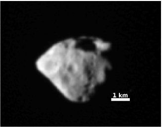
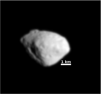
Figure 1: WAC image (left) at the close approach. The image was acquired with a narrow passband filter with central wavelength of 295.9 nm and FWHM=10.9 nm. The spatial resolution is 80 m/px. Since craters close to the limb are not easily detectable, the actual region used for crater count is reduced by one pixel around the limb. The pit-chain is clearly visible close to the right-hand terminator. The NAC image (right) shows the large depression which is approximately in the antipodal position of the alignment of pits and Ruby crater. The image was acquired with a narrow passband filter with central wavelength of 805.3 nm and FWHM=84.5 nm. The spatial resolution is 98 m/px.

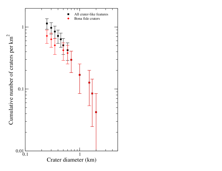
Figure 2: Cumulative distribution of all crater-like features and bona fide craters. The latter is the distribution used in the rest of the paper for age assessment. Both distributions contain features $\geq 3$ pixels (see Besse, 2010, for more details). Notice that the bona fide craters distribution does not contain the depressions forming the chain-like features (see text for details) and a couple of uncertain craters close to the Ruby’s rim. The resulting distribution shows a remarkable paucity of small ($D<0.5-0.6$ km) craters when compared to the distribution of all detected crater-like features. Error bars are estimated on the basis of Poisson statistics of counts.

A total of 42 crater-like features with dimensions ranging from about 0.2 to 2.1 km have been identified on three WAC images obtained near closest approach and one NAC image obtained about 10 min before CA (see fig. 1). However, the illumination conditions of the WAC images were considerably different from those of the NAC. Therefore in the present work, we restrict the analysis to the WAC images only. The effective area over which counts have been performed is 23.7 km², or approximately 25% of the estimated total Steins’ surface of 97.6 km² (for more details on crater identification and size estimate see Besse, 2010).
A total of 29 crater-like features larger than 3 pixels, ranging from about 0.24 km to 2.1 km, have been identified and used for the present work. The largest crater (named Ruby hereinafter) has a diameter of 2.1 km. The true nature of some features is uncertain. In particular, this is the case for a feature consisting of 8 pits aligned along a straight chain crossing a large degraded crater and extending almost from the south to the north pole of the asteroid. Owing to lack of sufficient resolution, it is not clear whether or not these aligned pits are due to impacts. The probability for such a chain of impacts to occur on a low gravity body like Steins is indeed extremely low. Moreover, a NAC image (see fig. 1 bottom panel), obtained from a different aspect, shows the presence of a large depression and an array of rimless circular pits, continuing the pit-chain imaged by the WAC (Keller et al., 2010). Therefore, the series of aligned depressions are most likely not caused by individual impacts. An alternative explanation is that the impact forming the crater Ruby triggered the nucleation of a long fracture or fault, whose expression at the surface is the pit-chain. Similar linear features were also observed on other small bodies, like Gaspra (Belton et al., 1992). Other uncertain crater-like features are located close to the rim of the Ruby crater (Besse, 2010).
The cumulative distributions of all detected crater-like features and 18 bona fide craters are reported in fig. 2. The latter has been constructed rejecting all the uncertain craters described above. Note that the small bona fide craters ($D<0.5-0.6$ km) are strongly underrepresented with respect to the distribution of the crater-like features.
The population of craters shows a wide range of depth-to-diameter ratios, varying from very shallow craters ($\sim 0.05$) to deep craters ($\sim 0.25$). The average crater depth-to-diameter ratio is $0.12\pm 0.05$ (Besse, 2010). Small craters have typically a lower depth-to-diameter ratio. These characteristics are consistent with crater degradation due to ejecta blanketing and/or disturbance of loose regolith on the surface triggered by impact seismic shaking (Richardson et al., 2005), in agreement with results for Itokawa (Hirata et al., 2009). Furthermore, Ruby has sharper rims and a higher depth-to-diameter ratio ($>0.14$; the bottom of the crater is not visible in the images) than several impact craters. Concerning the size distribution of Steins’ surface material, the modeling of the observed strong opposition effect and the overall photometric properties suggest that Steins may be covered by a layer of regolith having a mean particle size of $\sim 100$ $\mu$m. In the light of these considerations, the observed large degree of crater degradation may be explained in terms of regolith blanketing, i.e. deepest and sharpest craters are younger than more degraded ones.

3 The impactor flux

The flux of impactors can be expressed in terms of a differential distribution, $\phi(d,v)$, which represents the number of incoming bodies per unit of impactor size ($d$), impact velocity ($v$) and per unit time. Such a differential distribution, under the assumption that the impact velocity is independent on the impactor size, can be written as:

$$\phi(d,v)=h(d)f(v)$$ (1)

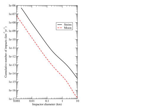
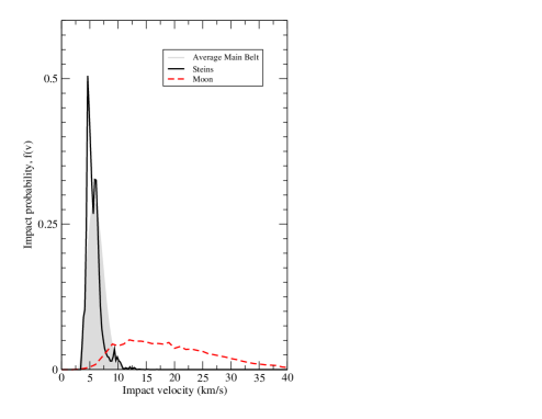
Figure 3: Steins’ cumulative impactor size distribution (upper panel) and impact velocity distribution (lower panel) used in the present work. For a comparison, the lunar impact distributions are also shown (Marchi et al., 2009).

where $h(d)$ is the impactor differential size distribution, and $f(v)$ is the distribution of impact velocity (i.e. impact probability per unit impact velocity) normalized to $\int f(v)\,dv\equiv 1$ (see Marchi et al., 2005, 2009, for details). In principle, the impactor size distribution could be derived from observations. At the small size range relevant for Steins ($d<1$ km), however, there is too little observational information to enable such an approach. To overcome such lack of information, we use the average size distribution of the main belt model derived by Bottke et al. (2005b, a). The estimated number of impactors at Steins is then obtained by multiplying the average size distribution by the intrinsic probability of collision with Steins, $P_{i}$ (see fig. 3 upper panel). The latter, evaluated by taking into account the observed orbital distribution of main belt asteroids, is $P_{i}=2.87\cdot 10^{-18}$ km^-2yr^-1, nearly equal to the main belt average intrinsic probability of collision. The impact velocity distribution $f(v)$ for Steins has been evaluated considering the population of main belt asteroids that presently intersect its orbit (see fig. 3 lower panel).Computations have been done using the Farinella & Davis (1992) algorithm. The resulting average impact velocity is 5.7 km/s.

4 The scaling law

The impactor flux is converted into a cumulative crater distribution (the so-called Model Production Function, MPF) using a scaling law (SL). The physics of the cratering processes for small asteroids is still poorly known. In this work we use the most updated SL derived from experimental analysis (Holsapple and Housen, 2007) and hydrocode simulations (Nolan et al., 1996). The SL for cratering on asteroids depends on several parameters, the most important being the internal structure and tensile strength ($Y$). Both are unknown for Steins. However, some constraints can be obtained from morphological studies.
Let us first consider the Holsapple and Housen (2007) scaling laws (HSL, hereinafter). An interesting issue concerns the minimum impactor dimension for catastrophic disruption ($d_{cd}$) of Steins. Assuming that Steins is an unfractured silicate rock and using the relevant specific energy for disruption, $Q^{*}_{D}=1-2\cdot 10^{7}$ erg/g (Holsapple, 2009), we derive that an impact at an average modulus velocity of 5.7 km/s with a body having size $d_{cd}=0.20-0.25$ km would be sufficient for catastrophic disruption. Moreover, for an unfractured rock with surface gravity $g$ and density $\rho$, the transition from strength to gravity cratering occurs at a crater diameter of $\sim 0.8Y/g\rho$ (Asphaug et al., 1996), which exceeds the size of the Ruby crater, except the cases of unreasonably low $Y$ values for a silicate body (namely $<10^{5}$ erg/g). Therefore, using HSL the strength regime applies. Under these conditions, we obtain that a 2 km crater is produced by an impactor having $d\sim d_{cd}$.
In this respect it is interesting to note that even though the visual appearance of Steins is dominated by the big Ruby crater, the ratio of largest crater diameter to average asteroid diameter of 0.38 is not particularly high. Asteroids Ida (0.44), Mathilde (0.62), and Vesta (0.87) reach considerably larger values (Asphaug, 2008). However, if compared to the specific energy required to disrupt the body, the big crater of Steins stands out (Fig. 4). Therefore the existence of the Ruby crater may be an indirect evidence that Steins was not a solid rock at the time of Ruby formation. Even if a particular tuning of the parameters may leave open such a possibility, it is more likely that Steins was a rubble pile or a collection of cohesive rubble of rocks. In the first case, for a pure cohesiveless rubble pile the gravity scale would apply. In the latter case, a cohesive rock scaling law may be more suitable. Concerning the present state of Steins, it is likely a rubble pile independently of its state prior to the formation of Ruby (Jutzi et al., 2010). This conclusion is also in agreement with the two large fracture-like features seen on its surface (see previous sections). A preliminary study of the formation of Ruby crater has been recently performed via numerical modeling (Jutzi et al., 2010). It has been found that a rubble pile body with some micro-porosity would have survived the formation of the Ruby crater, although the non-porous monolithic body hypothesis cannot be ruled out.
A further indication in favor of the rubble pile (both cohesiveless or with some low cohesion) nature of Steins may come from its shape, possibly due to YORP spin-up (Keller et al., 2010).
In conclusion, from previous reasoning, we limit our investigations to HSL for cohesive soils, and test the effects of different tensile strength. As a limiting case of a strengthless material we use the HSL for water (Holsapple and Housen, 2007). These equations read:

$$D=kd\biggl{(}\frac{Y}{\rho v_{\perp}^{2}}\biggr{)}^{\frac{\mu}{2}}\biggl{(}\frac{\rho}{\delta}\biggr{)}^{\nu}$$ (2)

$$D=kd\biggl{(}\frac{gd}{2v_{\perp}^{2}}\biggr{)}^{-\frac{\mu}{2+\mu}}\biggl{(}\frac{\rho}{\delta}\biggr{)}^{-\frac{2\nu}{2+\mu}}$$ (3)

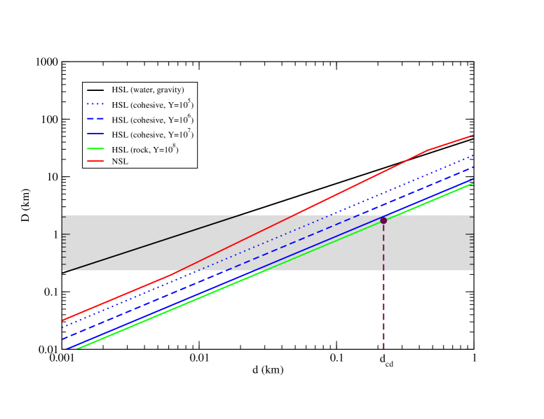
Figure 5: Relationship between impactor diameter ($d$) and crater diameter ($D$) according to the scaling laws discussed in this work. We also indicated the approximate impactor diameter for catastrophic disrupt ($d_{cd}$) of Steins, obtained for an unfractured silicate body and HSL. The limiting case of the water scaling law (not used for dating purposes) is shown only for a comparison. The gray area indicates the crater size range detected on Steins.

respectively for cohesive soils and water. $D$ is the crater diameter, $v_{\perp}$ is the normal component of the impact velocity, $\delta$ is the impactor density, $k,\mu,\nu$ depend on the material and are derived from experiments. Their numerical values are $k=1.03,1.17,\mu=0.41,0.55,$ respectively for Eq. 2 and Eq. 3, while $\nu=0.4$ in all cases (Holsapple and Housen, 2007). Concerning the strength, we may regard typical lunar regolith ($Y\sim 10^{5}$ dyne/cm²) and bulk silicates ($Y\sim 10^{8}$ dyne/cm²) as limiting cases for a silicate body. Highly under-dense (porous), aggregate materials having $Y<10^{5}$ dyne/cm² can be ruled out because of Steins’ stony composition (E-type). Concerning the higher limit, a more realistic estimate of the strength for an asteroid may be obtained considering that the strength depends on the asteroid size $R$, with larger bodies being weaker than smaller ones of similar composition. Assuming that the strength scales as $R^{-1/3}$ (Asphaug et al., 1996), Steins’ hard rock strength may be as low as a few $Y\sim 10^{6}$ dyne/cm². In the light of previous reasoning, we restrict the following analysis to the HSL for cohesive soils (for two representative values of tensile strength, namely $Y=10^{5},10^{6}$ dyne/cm²). In fig. 5 the HSL obtained for different parameters are reported.
A different approach is that proposed by Nolan et al. (1996). They estimated the cratering scaling law (NSL, hereinafter) using hydrocode simulations. Their main result is the discovery of the so-called fracture regime, which occurs in between the two extreme situations represented by the strength and gravity regimes. Basically, small craters are formed in the classical way, with their size being controlled by the local strength. In large craters, on the other hand, the shock wave propagates ahead of the excavation flow, and therefore the material is totally fractured prior to its removal. If the amount of excavated material is large enough, the size of the resulting crater is controlled by the gravity. A NSL has been derived for Gaspra, which can be rescaled to other asteroids using the approach proposed by O’Brien et al. (2006). Note that in this scenario bodies can survive much larger impacts than predicted by HSL. NSL can be arranged in the following manner:

$$D=cd^{\alpha}\biggl{(}\frac{v}{v_{0}}\biggr{)}^{\beta}\biggl{(}\frac{g}{g_{0}}\biggr{)}^{\delta}$$ (4)

where $c$, $\alpha$, $\beta$ and $\delta$ have different values for the strength, fracture and gravity regimes. The transitions between strength to fracture regime and from fracture to gravity regime occur respectively at:

$$d_{sf}=d_{0}\biggl{(}\frac{v}{v_{0}}\biggr{)}^{\gamma}$$ (5)

$$d_{fg}=d_{1}\biggl{(}\frac{v}{v_{0}}\biggr{)}^{\phi}\biggl{(}\frac{g}{g_{0}}\biggr{)}^{\theta}$$ (6)

where $d_{0}$, $v_{0}$ and $g_{0}$ are parameters computed for Gaspra. Numerical coefficient used here (expressed in c.g.s. units) are: $c=35,26.61,161.4;\alpha=1,1.159,0.78;\beta=0.56,0.65,0.44;\delta=0,0,-0.22$ respectively for the strength, fracture and gravity regimes, while $\gamma=\phi=-0.56;\theta=-0.58$ for all cases. Finally, $d_{0}=560$ cm, $d_{1}=2.56\cdot 10^{4}$ cm, $v_{0}=5.0$ km/s $g_{0}=0.448$ cm/s². Figure 5 shows the NSL rescaled to Steins.
By comparing the SLs reported in fig. 5, a large degree of variation emerges. For a fixed impactor size $d$, the resulting crater diameter $D$ may vary by more than a factor of 10. However, if we restrict ourselves to the observed crater size range on Steins and to the most likely scaling laws (NSL and HSL for $10^{5}<Y<10^{6}$ dyne/cm²) the variation is within a factor of 3. The difference can be partly explained by the fact that NSL overestimates cratering efficiency since it neglects the shear resistance of materials (Nolan et al., 1996).

5 The model production function

Using the considerations described in previous sections, it is possible to compute the differential distribution ($\Phi(D)$) of the number of craters with respect to their diameters expressed per unit time and surface area. The MPF can be obtained by:

$${\rm MPF}(D)=\int_{D}^{\infty}\Phi(\tilde{D})d\tilde{D}$$ (7)

The distribution of craters for a given age $t$ is simply obtained by: ${\rm MPF}(D)\times t$. These equations implicitly assume that all craters accumulate over time without interfering with previously formed craters (i.e. no crater erasing) and that the flux is constant over time. The latter assumption, according to lunar chronology, is valid for ages less than $\sim 3.7$ Ga (e.g. Marchi et al., 2009). In figure 6 (upper panel) the fit of the MPF to Steins crater counting data is shown.
The first important result is that the shape of the cumulative distribution cannot be satisfyingly fitted in the available size range. In particular, when fitting craters larger than $\sim 0.6$ km, the smaller craters are strongly underrepresented. Similar kinks in the cumulative distribution have been observed elsewhere, in particular on the Moon and Mars (e.g. Hiesinger et al., 2002; Haruyama et al., 2009), and usually are attributed to episodes of crater erasing which are more effective for small diameters. A similar lack of small craters, but for sizes $<10$ m, has also recently been observed on Itokawa (Hirata et al., 2009; Michel et al., 2009). In fig. 6 (upper panel) the best fit for large crater diameters is shown. The corresponding age, derived by using the NSL is $0.1\pm 0.02$ Ga. This estimate is likely to represent a lower limit, since the NSL neglects shear resistance and therefore tends to overestimate the crater sizes (Nolan et al., 1996). The HSL derived age ranges from $0.28\pm 0.06$ Ga to $0.94\pm 0.2$ Ga, for $Y=10^{5},10^{6}$ dyne/cm², respectively. Model ages are determined through a $\chi^{2}$ fitting. Formal errors are estimated considering a variation of $\pm 30\%$ around the minimum $\chi^{2}$. The cratering process may be more complicated than assumed so far, in particular the MPF may vary over time. The main reason for such time dependence is that craters may erase over time. A number of processes responsible for crater erasing on small bodies have been indentified: local and global jolting, cumulative seismic shaking and superposition of craters (Greenberg et al., 1994, 1996; Richardson et al., 2004). Such effects can be modeled (O’Brien et al., 2006) and the resulting MPF can be written in the following manner (Marchi et al., 2009):

$${\rm MPF}(D,t)=\int_{D}^{\infty}\Phi(\tilde{D},t){\cal E}(\tilde{D},t)\,d\tilde{D}$$ (8)

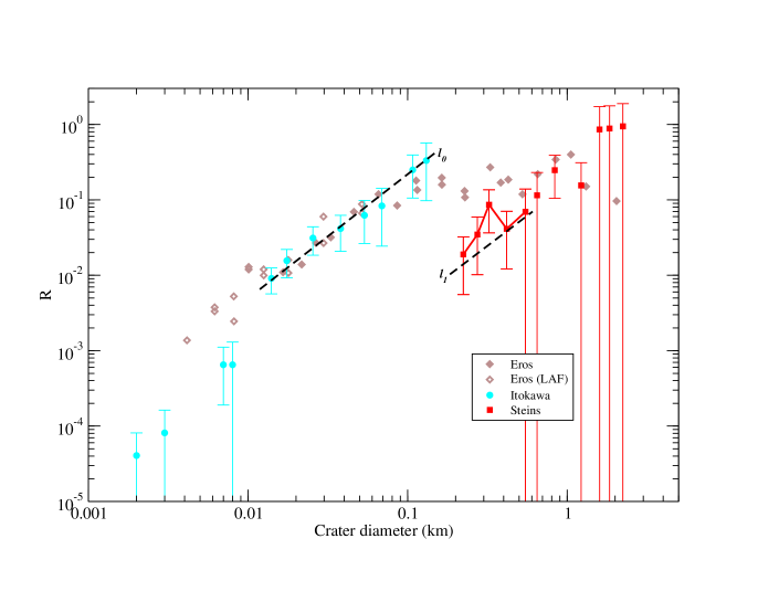
Figure 7: Steins’ crater data shown on a Relative plot (R-plot). R-values are computed according to Crater Analysis Techniques Working Group (1979). For comparison, Itokawa and Eros data are also shown. Itokawa data have been computed from table 1 of Hirata et al. (2009), while Eros data are from Chapman (2002). Dashed line $l_{o}$ indicates the average slopes for the left-most part of the Itokawa/Eros distributions ($D<0.15$ km), showing a paucity of small craters. For Itokawa and Eros this paucity of small craters has been interpreted as the result of seismic shaking (Richardson et al., 2004; Michel et al., 2009). Steins also shows a similar behavior (see line $l_{1}$ which is parallel to $l_{o}$) but for $D<0.35$ km the trend seems to have a steeper slope than Itokawa/Eros, possibly due to different processes of crater erasing (see text for details).

where the function ${\cal E}(D,t)$ is the ratio of the final number of craters, erasing included, to the total number (i.e. erasing excluded). The mentioned erasing process depends on several parameters. As for the regolith jolting and superposition, we use the parameters adopted in O’Brien et al. (2006) for Gaspra. Cumulative seismic shaking has not been applied in our simulations due to the lack of detailed information on regolith mobility on Steins.
Figure 6 (lower panel) shows the effects of crater erasing on Steins’ age determination. Also in this case, even though the MPF is shallower, the small craters are not accurately fitted by the models. Derived ages are now increased with respect to what was found neglecting crater erasing. Focusing again on $D>0.6$ km, we derive an age of $0.154\pm 0.035$ Ga for the NSL. In the case of the HSL, the age becomes $0.49\pm 0.18$ Ga and $1.6\pm 0.5$ Ga for $Y=10^{5},10^{6}$ dyne/cm², respectively.
We also investigated whether or not the observed crater population is saturated, i.e. has reached an equilibrium point where new craters erase old ones leaving unchanged the overall distribution. We find that the crater population has not yet reached saturation. To see this point, in figure 6 (lower panel) we overplot the MPF for 0.5 Ga (NSL) and 3.6 Ga (HSL). These ages have been chosen in order to have the corresponding MPFs above all the cumulative data points. Both MPFs are clearly separated by the best-fit curves, indicating that the saturation is not reached yet, therefore age assessment is possible.
It is interesting that also when taking into account the erasing of craters by superposition and regolith jolt, smaller craters are still strongly underrepresented. A number of possible explanations for the origin of this kink may be invoked. For instance, small craters may have been erased by regolith displacement due to the effect of cumulative seismic shaking. This process has been demonstrated to explain the deficit of small craters on Eros (Richardson et al., 2004) and Itokawa (Michel et al., 2009). In order to address this issue, we show the Steins’ crater distribution on a R-plot (see figure 7). R-plots are useful in order to analyze fine details of crater distributions. Data from Itokawa and Eros are also overplotted. The comparison among Itokawa, Eros and Steins is interesting mainly for the purpose of the small craters’ depletion, although, it is not so straightforward because of the different size range of craters. However, some interesting comments can still be drawn.
Itokawa and Eros show a marked depletion of small crater, for $D<0.1$ km. This fact has been interpreted as the result of crater erasing triggered by cumulative seismic shaking due to repeated small impacts (Richardson et al., 2004; Michel et al., 2009). This process is able to reproduce accurately the observed trend on Itokawa and Eros (indicated for clarity by the line $l_{o}$ in fig. 7).
As for Steins, the crater distribution for $D<0.5-0.6$ km shows an overall similar behavior, indicating that also on Steins the cumulative seismic shaking may be a viable explanation for the lack of small craters. Nevertheless there are some fine details that differ from Itokawa and Eros which are worth to be analyzed. To better show these discrepancies, in fig. 7 we draw the line $l_{1}$ which is parallel to $l_{0}$. Despite the large error bars, the 3 left-most bins ($D<0.3-0.4$ km) exhibit a steeper trend than that of Itokawa and Eros, although they might be compatible due to the relatively large statistical errors. This may be an indication that the erasing on Steins had a different origin, or at least that the cumulative shaking is not the unique responsible of the observed lack of small craters. We suggest that the Steins observed peculiar crater distribution could retain the footprint of an intense episode of erasing triggered be a single event, likely the formation of Ruby, which would have erased preferentially craters below $D\sim 0.3-0.4$ km. Note that the size bin corresponding to the Ruby crater in the cumulative distribution is close to the best fit model curve (see fig. 6). This means that the formation of such large craters is already accounted for by the model and yet this is not sufficient for explaining the lack of small craters, at least with the parameters used in this study. Therefore, we may argue that the formation of the Ruby crater happened in a more recent time than the best fit age.
An alternative explanation is connected to the YORP evolution that may have triggered regolith mobility and efficiently erased small craters (e.g. see Scheeres et al., 2007).
Without detailed knowledge of the internal nature of Steins and its regolith thickness it is very difficult to draw a firm conclusion. Nevertheless, erasing triggered by the Ruby impact seems more likely than the one induced by the YORP effect. This conclusion seems at least partially confirmed by the fresh appearance of the Ruby crater, with its sharp rims and high depth-to-diameter ratio.
In any case, we may use the crater distribution to constrain the epoch of the putative “impulsive erasing”. In order to correctly achieve this result a detailed knowledge of the erasing process is required. This is however far beyond the scopes of the present paper, hence we limit our discussion considering two cases. First of all, the case where all small craters ($D<0.35$ km) were erased at the same time. Through MPF fitting of the observed cumulative distribution for small craters, the approximate time lapsed since the erasing can be derived. Considering only the craters for $D<0.35$ km, for NSL we obtain an age of $0.032\pm 0.004$ Ga, which becomes $0.072\pm 0.01$ Gy and $0.237\pm 0.03$ Gy, for HSL and $Y=10^{5},10^{6}$ dyne/cm², respectively (see fig. 6, lower panel). Note, however, that the accumulations of craters during this time would have produced a steeper slope than the observed one resulting from face value of data points. Nevertheless, the statistical errors are too large to conclude whether or not the model distribution is really different to the observed trend. In this respect, it cannot be ruled out that seismic shaking might be entirely responsible for the slope of the crater size distribution in that size range, in this case the observed trend cannot be used to constrain the timescale of Ruby’s formation.
A lower limit for the epoch of the impulsive erasing can be derived considering that it erased most or all of the smallest craters ($D\sim 0.2-0.3$ km), but only some of the larger craters in order to reproduce the observed slope. In this case, the timescale could be set by the timescale to form just the smallest craters. The time required to accumulate the 4 observed craters having $D=0.2-0.3$ km spans from $\sim 2$ Ma to $\sim 10$ Ma, for NSL and HSLs respectively.
It is possible, using Poisson statistics, to compute the expected probabilities that the impulsive erasing due to Ruby formation occurred at the computed times. Assuming that during the crater retention ages the formation of only a single crater of the size of Ruby occurred, the probabilities that Ruby event occurred in the estimated recent times are: from $\sim$1 to $\sim$17% (NSL) and from $\sim$0.6 to $\sim$12% (HSL), respectively for the two different estimates of the impulsive event times reported above.
Another consequence of the formation of the Ruby crater would be the mixing of the regolith layer, with subsequent reset of the optical properties. It is interesting that detailed investigations across the surface of Steins have shown little or no spectral variability (Leyrat, 2010). This is somehow in contrast with other asteroids visited by spacecraft, all showing a certain degree of alteration due to space weathering (Chapman, 2004). The lack of spectral variability across Steins can be explained in different ways, although it must be noticed that space weathering response on E-type materials has not been investigated in details yet. A possibilty is that the lack of spectral variability may be an indication of Steins’ insensitive response to space weathering alteration due to its specific composition. However, as demonstrated by Lazzarin et al. (2006), all asteroidal spectral types are found to show some degree of alteration. In this case, Steins would have either a fresh or a totally saturated surface. The fresh surface scenario seems more likely given the fact that there is no spectral variation in proximity of small -and therefore relativey young- craters. This conclusion would be in agreement with the relatively young age estimated for the formation of the Ruby crater.

6 Conclusions

In this work we used crater counting, morphological analysis and impactor population modeling to constrain Steins’ cratering retention age. The derived ages vary according to the SLs used. In particular, using NSL and crater erasing the derived age is $0.154\pm 0.035$ Ga, while using HSL and crater erasing the age ranges from 0.49 to 1.6 Ga, according to the values of strength used. Moreover, the modeling of the crater erasing processes shows that the observed crater density is not saturated (at least for the parameters adopted here). The mean collisional age of Steins is estimated to be $\sim 2.2$ Ga (e.g. Marchi et al., 2006). Interestingly, similar numbers apply also for Gaspra. Analogue conclusions might be also valid for the near-Earth objects Eros, whose mean collisional age is $\sim 1.7$ Ga (Marchi et al., 2006) while cratering age using NSL gives 0.12 Ga (O’Brien et al., 2006) or, using HSL, 1-2 Ga (Michel et al., 2009). The larger bodies Ida and Mathilde have crater populations either close to the saturation or saturated, and consequently their cratering age estimate is less constrained. Despite the low number statistics, the cratering age of the main belt asteroids smaller than $\sim 20$ km seems to be systematically younger than their collisional age. This result, if confirmed by further studies, would have important implications on main belt collisional models.
Notably, the shape of Steins crater size distribution shows a kink for diameters smaller than 0.5-0.6 km, which may require a recent episode of intense erasing, although seismic shaking could have potentially played a role in producing the observed distribution as well. We also attempt to constrain the epoch of such episode, possibly associated to the Ruby crater formation. Focusing on the small diameter end ($D<0.35$ km) of the crater cumulative distribution, and adopting the MPF fitting we obtain an age of $0.032\pm 0.004$ Ga using NSL, from 0.072 to 0.237 Ga using HSL. Under the assumption that the formation of the Ruby crater erased all craters $<0.5-0.6$ km, the above ages could possibly indicate the time since the occurrence of the Ruby event. A lower limit to the age of this event, can be derived considering the time required to accumulate the observed craters in the range $0.2-0.3$ km. This produces an age from $\sim 2$ Ma to $\sim 10$ Ma, for NSL and HSLs respectively.
The derived ages vary up to a factor of ten depending on the SL and the tensile strength used. In the present work we investigated the effects of a relatively large range of SLs and $Y$. However, in the light of our global understanding of Stein properties, we favor a crater retention age ranging from $\sim 0.15$ to $\sim 0.5$ Ga, and a kink related event that could be as young as a few Ma up to some tens of Ma.
As a final remark, note that the conclusions derived in this paper are based on the bona fide crater distribution. The general scenario outlined (age, depletion of small craters) remains valid also if considering all crater-like features (see fig. 6, lower panel). In the latter case, however, the age of the reset event is about a factor of two higher.

Acknowledgment

We thank A. Morbidelli for providing us with the impact probability file for Steins. We are also grateful to the referee D. O’Brien for many helpful comments and for providing us the published data of Itokawa and Eros cratering record. Thanks also to a second anonymous referee for insightful suggestions. Finally, we thank E. Simioni and E. Martellato for discussions.

Figure 4: The ratio of the diameter of the biggest crater divided by the average diameter of various asteroids (triangles, left ordinate) and the third root of the specific energy for disruption (diamonds) and shattering (asterisks) of a basaltic body impacted with a velocity of 5 km/s (Benz and Asphaug, 1999, right ordinate). The relation between the left and right ordinate is arbitrary. The critical impact is expected to be between the shattering and the disruption limit. For Steins we used an average diameter of 5.3 km, a size of the largest crater of 2 km and assumed a density (needed for the energy of disruption) of 2 g/cm³. Data for the other asteroids are taken from Asphaug (2008). For Amalthea and Vesta the specific energy of disruption is above the plot range. The figure shows that the ratio between size of the largest crater and body size is not particularly high on Steins. However, since the energy needed to shatter a body is at a minimum at approximately the size of Steins, an impactor large enough to create the Ruby crater would be expected to shatter (but not necessarily disrupt) Steins. The model calculations by Jutzi et al. (2010) suggest that this actually may have been the case: In many cases an impactor of the size needed to create the Ruby crater will strongly damage the original body, but Steins’ global shape will remain approximately the same and after the event the crater will be clearly visible.

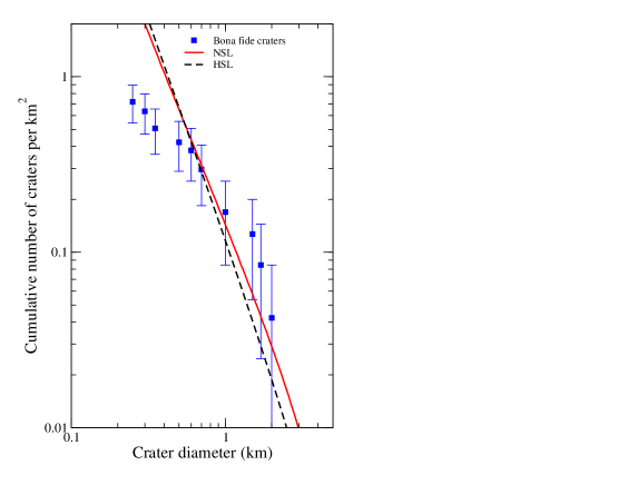
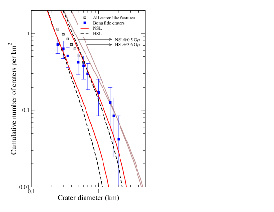
Figure 6: Upper panel: Steins’ age estimates obtained with the MPF and no crater erasing. The best fits have been performed considering only craters for $D>0.6$ km. Notice the strong lack of observed craters for $D<0.6$ km in comparison to the models. Lower panel: Steins’ age estimates obtained with the MPF and crater erasing. The best fits for small diameters ($D<0.35$ km) is also shown, possibly indicating the time of the formation of the Ruby crater (see text for further details). For a comparison, the distribution of all crater-like features is also shown (errors bars are not shown for simplicity, see Fig. 2). To adreess the crater saturation issue a couple of MPFs for older ages have been also overplotted (see text).

References

- Asphaug (2008) Asphaug, E., Sep. 2008. Critical crater diameter and asteroid impact seismology. Meteoritics and Planetary Science 43, 1075–1084.
- Asphaug et al. (1996) Asphaug, E., Moore, J. M., Morrison, D., Benz, W., Nolan, M. C., Sullivan, R. J., Mar. 1996. Mechanical and Geological Effects of Impact Cratering on Ida. Icarus 120, 158–184.
- Belton et al. (1994) Belton, M. J. S., Chapman, C. R., Veverka, J., Klaasen, K. P., Harch, A., Greeley, R., Greenberg, R., Head, III, J. W., McEwen, A., Morrison, D., Thomas, P. C., Davies, M. E., Carr, M. H., Neukum, G., Fanale, F. P., Davis, D. R., Anger, C., Gierasch, P. J., Ingersoll, A. P., Pilcher, C. B., Sep. 1994. First Images of Asteroid 243 Ida. Science 265, 1543–1547.
- Belton et al. (1992) Belton, M. J. S., Veverka, J., Thomas, P., Helfenstein, P., Simonelli, D., Chapman, C., Davies, M. E., Greeley, R., Greenberg, R., Head, J., Sep. 1992. Galileo encounter with 951 Gaspra - First pictures of an asteroid. Science 257, 1647–1652.
- Benz and Asphaug (1999) Benz, W., Asphaug, E., Nov. 1999. Catastrophic Disruptions Revisited. Icarus 142, 5–20.
- Besse (2010) Besse, S. et al. 2010. xxxxxxx. Icarus, submitted.
- Bottke et al. (2005a) Bottke, W. F., Durda, D. D., Nesvorný, D., Jedicke, R., Morbidelli, A., Vokrouhlický, D., Levison, H., May 2005a. The fossilized size distribution of the main asteroid belt. Icarus 175, 111–140.
- Bottke et al. (2005b) Bottke, W. F., Durda, D. D., Nesvorný, D., Jedicke, R., Morbidelli, A., Vokrouhlický, D., Levison, H. F., Dec. 2005b. Linking the collisional history of the main asteroid belt to its dynamical excitation and depletion. Icarus 179, 63–94.
- Chapman (2002) Chapman, C. R., 2002. Cratering on Asteroids from Galileo and NEAR Shoemaker. Asteroids III, 315–329.
- Chapman (2004) Chapman, C. R., May 2004. Space Weathering of Asteroid Surfaces. Annual Review of Earth and Planetary Sciences 32, 539–567.
- Crater Analysis Techniques Working Group (1979) Crater Analysis Techniques Working Group, 1979. Standard techniques for presentation and analysis of crater size-frequency data. Icarus, 37, 467.
- Farinella & Davis (1992) Farinella, P., & Davis, D. R., 1992. Collision rates and impact velocities in the Main Asteroid Belt. Icarus, 97, 111.
- Greenberg et al. (1996) Greenberg, R., Bottke, W. F., Nolan, M., Geissler, P., Petit, J., Durda, D. D., Asphaug, E., Head, J., Mar. 1996. Collisional and Dynamical History of Ida. Icarus 120, 106–118.
- Greenberg et al. (1994) Greenberg, R., Nolan, M. C., Bottke, Jr., W. F., Kolvoord, R. A., Veverka, J., Jan. 1994. Collisional history of Gaspra. Icarus 107, 84–+.
- Haruyama et al. (2009) Haruyama, J., Ohtake, M., Matsunaga, T., Morota, T., Honda, C., Yokota, Y., Abe, M., Ogawa, Y., Hideaki, M., Iwasaki, A., Pieters, C. M., Asada, N., Demura, H., Hirata, N., Terazono, J., Sasaki, S., Saiki, K., Yamaji, A., Torii, M., Josset, J., Feb. 2009. Long-Lived Volcanism on the Lunar Farside Revealed by SELENE Terrain Camera. Science 323, 905–908.
- Hiesinger et al. (2002) Hiesinger, H., Head III, J.W., Wolf, U., Jaumann, R., Neukum, G., 2002. Lunar mare basalt flow units: Thicknesses determined from crater size-frequency distributions. Geophys. Res. Lett. 29, 1248.
- Hirata et al. (2009) Hirata, N., Barnouin-Jha, O. S., Honda, C., Nakamura, R., Miyamoto, H., Sasaki, S., Demura, H., Nakamura, A. M., Michikami, T., Gaskell, R. W., Saito, J., Apr. 2009. A survey of possible impact structures on 25143 Itokawa. Icarus 200, 486–502.
- Holsapple (2009) Holsapple, K. A., Feb. 2009. On the strength of the small bodies of the solar system: A review of strength theories and their implementation for analyses of impact disruptions. Planetary and Space Science 57, 127–141.
- Holsapple and Housen (2007) Holsapple, K. A., Housen, K. R., Mar. 2007. A crater and its ejecta: An interpretation of Deep Impact. Icarus 187, 345–356.
- Jutzi et al. (2010) Jutzi, M., Michel, P., Benz, W. 2010. A large crater as a probe of the internal structure of the E-type asteroid Steins. A&A 509, L2.
- Keller et al. (2010) Keller, H. U. et al. 2010. E-Type Asteroid (2867) Steins as Imaged by OSIRIS on Board Rosetta. Science 327, 190.
- Keller et al. (2007) Keller, H. U., Barbieri, C., Lamy, P., Rickman, H., Rodrigo, R., Wenzel, K., Sierks, H., A’Hearn, M. F., Angrilli, F., Angulo, M., Bailey, M. E., Barthol, P., Barucci, M. A., Bertaux, J., Bianchini, G., Boit, J., Brown, V., Burns, J. A., Büttner, I., Castro, J. M., Cremonese, G., Curdt, W., da Deppo, V., Debei, S., de Cecco, M., Dohlen, K., Fornasier, S., Fulle, M., Germerott, D., Gliem, F., Guizzo, G. P., Hviid, S. F., Ip, W., Jorda, L., Koschny, D., Kramm, J. R., Kührt, E., Küppers, M., Lara, L. M., Llebaria, A., López, A., López-Jimenez, A., López-Moreno, J., Meller, R., Michalik, H., Michelena, M. D., Müller, R., Naletto, G., Origné, A., Parzianello, G., Pertile, M., Quintana, C., Ragazzoni, R., Ramous, P., Reiche, K., Reina, M., Rodríguez, J., Rousset, G., Sabau, L., Sanz, A., Sivan, J., Stöckner, K., Tabero, J., Telljohann, U., Thomas, N., Timon, V., Tomasch, G., Wittrock, T., Zaccariotto, M., Feb. 2007. OSIRIS The Scientific Camera System Onboard Rosetta. Space Science Reviews 128, 433–506.
- Lazzarin et al. (2006) Lazzarin, M., Marchi, S., Moroz, L. V., Brunetto, R., Magrin, S., Paolicchi, P., Strazzulla, G., Aug. 2006. Space Weathering in the Main Asteroid Belt: The Big Picture. Astrophysical Journal Letters 647, L179–L182.
- Leyrat (2010) Leyrat, C. et al, 2010. xxxxxxx. PSS this issue 00, 0–0.
- Marchi et al. (2005) Marchi, S., Morbidelli, A., Cremonese, G., Mar. 2005. Flux of meteoroid impacts on Mercury. Astronomy & Astrophysics 431, 1123–1127.
- Marchi et al. (2009) Marchi, S., Mottola, S., Cremonese, G., Massironi, M., Martellato, E., Jun. 2009. A New Chronology for the Moon and Mercury. Astronomical Journal 137, 4936–4948.
- Marchi et al. (2006) Marchi, S., Paolicchi, P., Lazzarin, M., Magrin, S., Feb. 2006. A General Spectral Slope-Exposure Relation for S-Type Main Belt and Near-Earth Asteroids. Astronomical Journal 131, 1138–1141.
- Michel et al. (2009) Michel, P., O’Brien, D. P., Abe, S., Hirata, N., Apr. 2009. Itokawa’s cratering record as observed by Hayabusa: Implications for its age and collisional history. Icarus 200, 503–513.
- Nolan et al. (1996) Nolan, M. C., Asphaug, E., Melosh, H. J., Greenberg, R., Dec. 1996. Impact Craters on Asteroids: Does Gravity or Strength Control Their Size? Icarus 124, 359–371.
- O’Brien et al. (2006) O’Brien, D. P., Greenberg, R., Richardson, J. E., Jul. 2006. Craters on asteroids: Reconciling diverse impact records with a common impacting population. Icarus 183, 79–92.
- Richardson et al. (2004) Richardson, J. E., Melosh, H. J., Greenberg, R., Nov. 2004. Impact-Induced Seismic Activity on Asteroid 433 Eros: A Surface Modification Process. Science 306, 1526–1529.
- Richardson et al. (2005) Richardson, J. E., Melosh, H. J., Greenberg, R. J., O’Brien, D. P., Dec. 2005. The global effects of impact-induced seismic activity on fractured asteroid surface morphology. Icarus 179, 325–349.
- Saito et al. (2006) Saito, J., Miyamoto, H., Nakamura, R., Ishiguro, M., Michikami, T., Nakamura, A. M., Demura, H., Sasaki, S., Hirata, N., Honda, C., Yamamoto, A., Yokota, Y., Fuse, T., Yoshida, F., Tholen, D. J., Gaskell, R. W., Hashimoto, T., Kubota, T., Higuchi, Y., Nakamura, T., Smith, P., Hiraoka, K., Honda, T., Kobayashi, S., Furuya, M., Matsumoto, N., Nemoto, E., Yukishita, A., Kitazato, K., Dermawan, B., Sogame, A., Terazono, J., Shinohara, C., Akiyama, H., Jun. 2006. Detailed Images of Asteroid 25143 Itokawa from Hayabusa. Science 312, 1341–1344.
- Scheeres et al. (2007) Scheeres, D. J., Abe, M., Yoshikawa, M., Nakamura, R., Gaskell, R. W., Abell, P. A. 2007. The effect of YORP on Itokawa. Icarus 188, 425–429.
- Veverka et al. (1999a) Veverka, J., Thomas, P., Harch, A., Clark, B., Bell, J. F., Carcich, B., Joseph, J., Murchie, S., Izenberg, N., Chapman, C., Merline, W., Malin, M., McFadden, L., Robinson, M., Jul. 1999a. NEAR Encounter with Asteroid 253 Mathilde: Overview. Icarus 140, 3–16.
- Veverka et al. (1999b) Veverka, J., Thomas, P. C., Bell, III, J. F., Bell, M., Carcich, B., Clark, B., Harch, A., Joseph, J., Martin, P., Robinson, M., Murchie, S., Izenberg, N., Hawkins, E., Warren, J., Farquhar, R., Cheng, A., Dunham, D., Chapman, C., Merline, W. J., McFadden, L., Wellnitz, D., Malin, M., Owen, Jr., W. M., Miller, J. K., Williams, B. G., Yeomans, D. K., Jul. 1999b. Imaging of asteroid 433 Eros during NEAR’s flyby reconnaissance. Science 285, 562–564.