On the weak confinement of kinks in the one-dimensional quantum ferromagnet $\mathrm{Co}\mathrm{Nb}_{2}\mathrm{O}_{6}$

Abstract

In a recent paper Coldea et al(2010 Science 327 177) report observation of the weak confinement of kinks in the Ising spin chain ferromagnet $\mathrm{Co}\mathrm{Nb}_{2}\mathrm{O}_{6}$ at low temperatures. To interpret the entire spectra of magnetic excitations measured via neutron scattering, they introduce a phenomenological model, which takes into account only the two-kink configurations of the spin chain. We present the exact solution of this model. The explicit expressions for the two-kink bound-state energy spectra and for the relative intensities of neutron scattering on these magnetic modes are obtained in terms of the Bessel function.

1 Introduction

Very recently Coldea et al[1] reported the impressive results of inelastic neutron scattering experiments on the quasi-1D ferromagnetic $\mathrm{Co}\mathrm{Nb}_{2}\mathrm{O}_{6}$ (cobalt niobate) single crystal. The essential physics of this material at low temperatures can be described in terms of the quantum Ising spin chain model, which is paradigmatic for the theory of the quantum phase transitions [2]. In presence of the magnetic field $h_{\perp}$ transverse to the easy magnetization axis, the ground state state of the model can be either ferromagnetic or paramagnetic depending on the strength of the external magnetic field $h_{\perp}$. The transition between the two phases occurs (at zero temperature) at the critical value of the transverse field $h_{\perp}=h_{c}$. This critical point belongs to the 2D Ising universality class.

The spectra observed by Coldea et al[1] display certain very subtle features providing experimental confirmation of two long-standing theoretical predictions [3, 4], which relate to the Ising model. Directly at the critical transverse field $h_{\perp}=h_{c}=5.5T$, the ratio of two lightest quasiparticles approaches to the ’golden ratio’ indicating the hidden $E_{8}$ symmetry in the critical Ising model in the longitudinal magnetic field, as it was predicted by A.B. Zamolodchikov [4] nearly two decades ago. On the other hand, at zero magnetic field, the observed energies of five lowest magnetic excitations were proportional to the absolute values $z_{n}$ of zeroes of the Airy function, $\mathrm{Ai}(-z_{n})=0$, in agreement with the theory of the kink confinement originating in 1978 from the work of McCoy and Wu [3]. On the resent developments in this field see [5, 6, 7, 8, 9, 10, 11], further references can be found in the monograph [12].

Confinement of topological excitations typically takes place in two dimensions (one spacial and one time dimension), if the discrete vacuum degeneracy is explicitly broken by a small interaction term. In the simplest heuristic approach, two confined kinks in the ferromagnetic Ising chain are treated as two quantum particles moving in a line $-\infty<x<\infty$ and attracting one another with a linear potential $\lambda|x|$. The latter can be induced in the quasi-1D Ising ferromagnet either by a weak external longitudinal magnetic field, or by the weak coupling between the magnetic chains in the 3D magnetically ordered phase [1, 13, 14]. In this approach, the relative motion of two kinks is described by the Schrödinger equation

$$-\frac{1}{m}\frac{d^{2}}{dx^{2}}\psi_{n}(x)+\lambda|x|\psi_{n}(x)=\delta E_{n}\,\psi(x),$$ (1)

with a skew-symmetric wave function $\psi(x)=-\psi(-x)$. It immediately leads to the energy levels of the kink bound-states [3]

$$\delta E_{n}=z_{n}\lambda^{2/3}m^{-1/3},\quad n=1,2\ldots$$ (2)

The simple theory of confinement based on (2) implies the quadratic dispersion law $p^{2}/(2m)$ for a free kink, and ignores discreteness of the spin chain. Though these approximations are reasonable for small enough momenta of the composite two-kink bound states, a more systematic approach is required to describe their spectra in the whole Brillouin zone.

The effect of the lattice discreteness on the kink confinement in the non-critical Ising spin chain has been studied in ref. [16] in the Bethe-Salpeter equation approach [7, 8]. To interpret the full experimental spectra in $\mathrm{Co}\mathrm{Nb}_{2}\mathrm{O}_{6}$, Coldea and his colleagues proposed a different phenomenological model, which takes into account only the two-kink (i.e. one-domain) configurations of the spin chain. The Hamiltonian of this model is given in [17] by equation (S1), which we reproduce in equation (3) below. The neutron scattering spectra were compared by authors of ref. [1] with an approximate perturbative solution [18] of their phenomenological model. It is interesting, that this model admits an exact solution, which we describe in the present paper. Our main results are equations (24), (25), and (44), which express the energy spectra and relative neutron-scattering intensities of the magnetic excitation modes for model (3) in terms of the Bessel function.

The rest of the paper is organized as follows. In Section 2 the phenomenological model introduced in [17] is described and its exact energy spectrum is obtained. These exact spectra are analyzed in several asymptotical regimes in the small magnetic field limit in Section 3. Section 4 contains calculation of the dynamical correlation function, which is proportional to the neutron-scattering intensities. The details of calculations are described in two Appendices. Concluding remarks are presented in Section 5.

2 The two-kink model and its energy spectrum

In this Section we study the eigenvalue problem for the model Hamiltonian defined by equation (S1) of [17]:

$$H|j,l\rangle=J|j,l\rangle-\alpha[|j,l+1\rangle+(|j,l-1\rangle+|j+1,l-1\rangle)(1-\delta_{l,1})$$

$$+|j-1,l+1\rangle]+h_{z}l|j,l\rangle-\beta\delta_{l,1}(|j-1,1\rangle+|j+1,1\rangle)+\beta^{\prime}|j,1\rangle\delta_{l,1}.$$ (3)

Here $|j,l\rangle$ denotes the two-kink state of the ferromagnetic spin-$1/2$ chain,

$$|j,l\rangle=|\ldots\uparrow\uparrow\uparrow\stackrel{{\scriptstyle j}}{{\downarrow}}\downarrow\ldots\downarrow\stackrel{{\scriptstyle j+l}}{{\uparrow}}\uparrow\uparrow\ldots\rangle,$$

the indices $j$ and $l$ give the starting position and the length of the down-spin cluster, $j=0,\pm 1,\pm 2,\ldots$, and $l=1,2,\ldots$ Parameter $J$ characterizes the energy needed to create two kinks. The terms proportional to $\alpha$ describe the nearest neighbour hoppings of kinks along the chain. The long-range attraction between the kinks is represented in (3) by the term $h_{z}l$, where $h_{z}$ is the effective longitudinal magnetic field. The short-range interaction $\beta$- and $\beta^{\prime}$-terms were introduced in [17] to describe the experimentally observed ’kinetic mode’ - the well localized bound-state mode near the Brillouin zone boundary [1]. Note, that $\beta$- and $\beta^{\prime}$-terms has no analogue in the standard Ising spin chain Hamiltonian.

In the momentum basis

$$|P,l\rangle=\sum_{j=-\infty}^{\infty}\exp(\rmi Pj)|j,l\rangle,$$ (4)

the Hamiltonian is diagonal in the momentum variable $P$ and acts on the basis state as follows

$$H|P,l\rangle=-\alpha[(1+e^{\rmi P})|P,l+1\rangle+(1-\delta_{l,1})(1+e^{-\rmi P})|P,l-1\rangle]+$$

$$[J+h_{z}l+(\beta^{\prime}-2\beta\cos P)\delta_{l,1}]|P,l\rangle.$$ (5)

The eigenvalue problem

$$H|\Phi(P)\rangle=E(P)|\Phi(P)\rangle$$ (6)

takes in basis (4) the explicit form

$$[J+h_{z}l+(\beta^{\prime}-2\beta\cos P)\delta_{l,1}-E(P)]\psi(l,P)-$$

$$-2\alpha\cos(P/2)[\psi(l+1,P)+(1-\delta_{l,1})\psi(l-1,P)]=0,$$ (7)

where $l=1,2,\ldots$, the momentum $P$ has the Brillouin zone $-\pi<P<\pi$, and

$$2\pi\,\delta(P^{\prime}-P)\,\psi(l,P)=\exp(-\rmi Pl/2)\langle P^{\prime},l|\Phi(P)\rangle.$$

Problem (6) can be easily solved in the case of zero magnetic field. The energy spectrum at $h_{z}=0$ has the continuous part

$$E(k,P)\equiv\varepsilon(k,P)=J-4\alpha\cos(P/2)\cos k,$$ (8)

and one localized bound state, the ’kinetic mode’,

$$E_{kin}(P)=J+(\beta^{\prime}-2\beta\cos P)+\frac{4\alpha^{2}\cos^{2}(P/2)}{\beta^{\prime}-2\beta\cos P}.$$ (9)

Note, that the wave functions corresponding to the continuous spectrum and to the kinetic bound state mode read, respectively, as

$$\psi(l,P;k)=A\,\sin[k(l-1)+\gamma],$$ (10)

$$\psi_{kin}(l,P)=B\,z^{l},$$ (11)

where $A$ and $B$ are the normalizing constants, and

$$z=\frac{2\alpha\cos(P/2)}{2\beta\cos P-\beta^{\prime}}\,,$$

$$\cot\gamma=\cot k+\frac{\beta^{\prime}-2\beta\cos P}{2\alpha\sin k\,\cos(P/2)}$$ (12)

Requirement $|z|<1$ implies, that the kinetic mode (11) exists only in the region near the Brillouin zone boundary, at

$$|\cos(P/2)|<\frac{-\alpha+(\alpha^{2}+8\beta^{2}+4\beta\beta^{\prime})^{1/2}}{2\beta}.$$ (13)

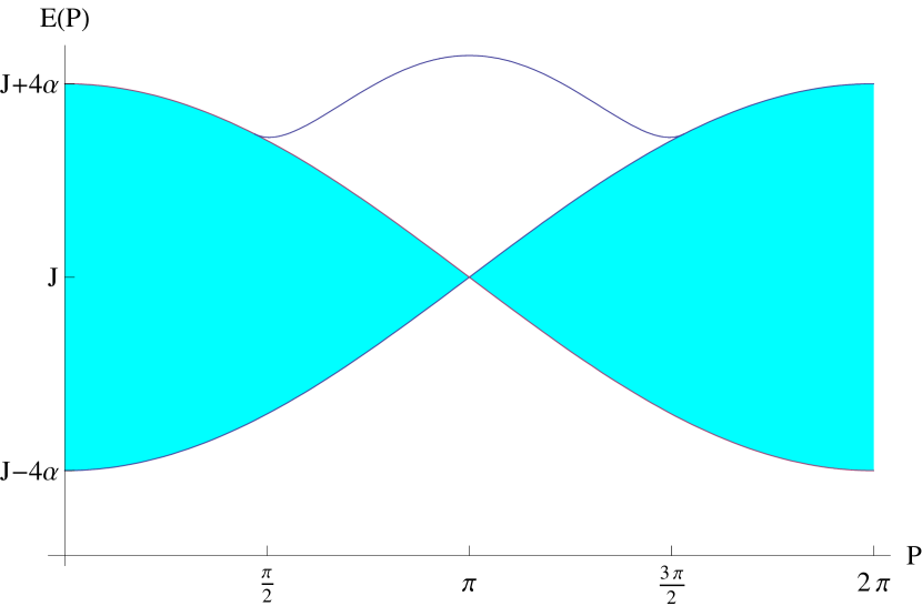
Figure 1: The energy spectrum of (7) at $h_{z}=0$, according to (8), (9). The filled area corresponds to the continuous spectrum.

At the edges of this region, the gap between the continuous spectrum and the kinetic mode vanishes. The resulting energy spectrum at $h_{z}=0$ is shown in Figure 1.

Returning to the original eigenvaule problem (7) with $h_{z}>0$, we rewrite it as follows

$$\left(-\lambda+\mu\,l+\frac{a\,\delta_{l,1}}{2}\right)\psi(l,P)-\frac{\psi(l+1,P)+(1-\delta_{l,1})\psi(l-1,P)}{2}=0,$$ (14)

where $l=1,2,\ldots$, the eigenfunction $\psi(l,P)$ vanishes at $l\to+\infty$, and

$$\lambda=\frac{E(P)-J}{4\alpha\cos(P/2)},\quad a=\frac{\beta^{\prime}-2\beta\cos P}{2\alpha\cos(P/2)},\quad\mu=\frac{h_{z}}{4\alpha\cos(P/2)}.$$ (15)

It is possible to extend equation (14) to all integer $l\in{\mathbb{Z}}$, not necessary positive. Let us continue $\psi(P,l)$ skew-symmetrically to negative $l$ denoting

$$\Psi(l,P)=\cases{\psi(l,P),&for\;$l=1,2,\ldots$ ,\\ 0,&for\;$l=0,$\\ -\psi(-l,P,),&for\;$l=-1,-2,\ldots$}$$ (16)

One can easily check then, that the odd (in $l$) function $\Psi(l,P)$ solves equation

$$\left(-\lambda+\mu\,|l|+\frac{a\,\delta_{|l|,1}}{2}\right)\Psi(l,P)-\frac{\Psi(l+1,P)+\Psi(l-1,P)}{2}=0,$$ (17)

for $l=0,\pm 1,\pm 2,\ldots$, iff the function $\psi(P,l)$ is the solution of the equation (14) for $l=1,2,\ldots$

After the Fourier transform, equation (17) takes the form

$$[\epsilon(z)-\lambda]\phi(z)+\frac{a}{2}\Psi(1)\left(z-\frac{1}{z}\right)=-\mu z\oint_{S_{1}}\frac{\rmd z^{\prime}}{\pi\rmi}\frac{\phi(z^{\prime})}{(z^{\prime}-z)^{2}},$$ (18)

$${\rm with}\;\;\epsilon(z)=-\frac{1}{2}\left(z+\frac{1}{z}\right),$$ (19)

$$\Psi(1)=\oint_{S_{1}}\frac{\rmd z}{4\pi\rmi z}\phi_{n}(z)\left(\frac{1}{z}-z\right).$$ (20)

Here $S_{1}$ denotes the unit circle in the complex plane, the both $z$ and $z^{\prime}$ variables lie in this circle, $|z|=|z^{\prime}|=1$. Integration in (18) is taken in the counter-clockwise direction and understood in the sense of the Cauchy principal value. The function $\phi(z)$ is defined as

$$\phi(z)\equiv\sum_{l=-\infty}^{\infty}z^{l}\,\Psi(l,P)=\sum_{l=1}^{\infty}(z-z^{-1})\,\psi(l,P),$$ (21)

and satisfies the symmetry property $\phi(1/z)=-\phi(z)$. We have dropped the explicit indication of the $P$-dependence in $\phi(z)$ and $\Psi(1)$, the full notation for these quantities should be $\phi(z,P)$ and $\Psi(1,P)$.

At $a=0$, problem (18) reduces to the First Toy Model, solved in Subsection 6.1 of [16]. At $a\neq 0$, problem (18) can be solved by the same method. The result for the eigenvalues $\lambda_{n}$ reads as

$$\lambda_{n}=-\mu\,\nu_{n},$$ (22)

where $\nu_{n}$ are the solutions of the equation

$$J_{\nu_{n}}(1/\mu)+a\,J_{\nu_{n}+1}(1/\mu)=0,$$ (23)

with $J_{\nu}(x)$ being the Bessel function of order $\nu$. In A, we describe an alternative proof of this result.

Accordingly, the solution of the eigenvalue problem (6) reads as

$$E_{n}(P)=J-h_{z}\,\nu_{n},$$ (24)

and $\nu_{n}$ are the solutions of equation

$$2\alpha\cos(P/2)J_{\nu_{n}}[4h_{z}^{-1}\alpha\cos(P/2)]+(\beta^{\prime}-2\beta\cos P)J_{\nu_{n}+1}[4h_{z}^{-1}\alpha\cos(P/2)]=0.$$ (25)

Figure 2 shows 30 lowest modes, calculated from (24), (25) with the Hamiltonian parameter values

$$J=1.94\,\,{\rm meV},\quad\alpha=0.12J,\quad\beta=0.17\,J,\quad\beta^{\prime}=0.21\,J,\quad h_{z}=0.02J,$$ (26)

chosen by Coldea et al[17] to give the best fit of the experimental results.

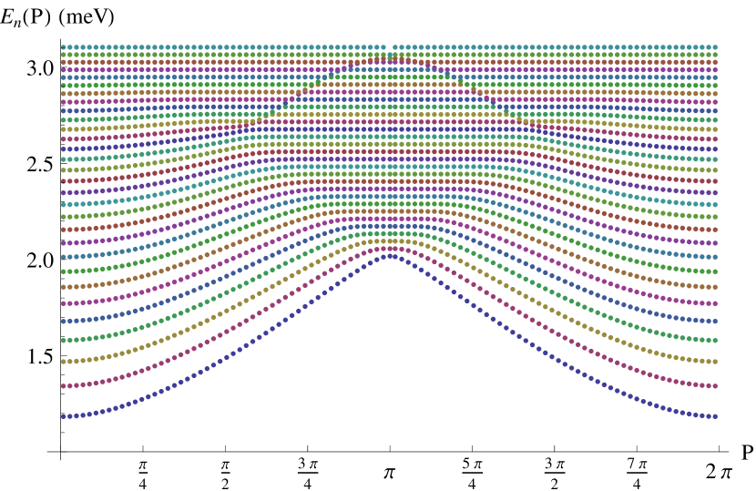
Figure 2: Energy spectra of 30 lightest modes calculated from (24), (25), (26).

3 Weak-$h_{z}$ expansions

If the longitudinal magnetic field is weak $h_{z}\to+0$, the long range confining potential $h_{z}l$ between the kinks becomes small. Corresponding asymptotic expansions for the spectra $E_{n}(P)$ of their bound sates can be extracted from the obtained exact results, either by means of appropriate asymptotic formulas for the Bessel functions, or by direct calculation of the integral in the left-hand side of equation [see equation (55)]

$$\int_{C}\rmd z^{\prime}\,\left(\frac{1}{z^{\prime}}+a\right)\exp\left\{\frac{\rmi}{\mu}[{\mathcal{F}}(z^{\prime})]\right\}=0,$$ (27)

by the saddle point method at $\mu\to+0$. Here ${\mathcal{F}}(z)=-\lambda\log z-\frac{1}{2}(z-z^{-1})$, and contour $C$ is shown in Fig. 8 in A. In this limit, one can distinguish several asymptotical regimes for different $n$ and $P$, depending on the location of the saddle points

$$z_{1,2}^{\prime}=-\lambda_{n}\pm\sqrt{\lambda_{n}^{2}-1}$$ (28)

in the $z^{\prime}$-plane in integral (27). Since these calculations are very similar to those described in [16], we present here only the final results.

3.1 Low energy expansion

If $n\sim 1$ and $P$ is well below the Brillouin zone boundary, $\lambda$ becomes close to $-1$, and the saddle points (28) merge at $z_{1,2}^{\prime}=1$. In this case, one can use the low energy expansion in fractional powers of $h_{z}$:

$$E_{n}(P)=J-4\alpha\cos(P/2)+[2\alpha\cos(P/2)]^{1/3}h_{z}^{2/3}z_{n}+$$ (29)

$$\frac{h_{z}\,(\beta^{\prime}-2\beta\cos P)}{\beta^{\prime}-2\beta\cos P+2\alpha\cos(P/2)}-\frac{h_{z}^{4/3}z_{n}^{2}}{60\,[2\alpha\cos(P/2)]^{1/3}}+O(h_{z}^{5/3}),$$

with $(-z_{n})$ being the zeros of the Airy function, ${\rm Ai}(-z_{n})=0$.

The analogous expansion for $\lambda_{n}$ reads as

$$\lambda_{n}=-1+\frac{\mu^{2/3}z_{n}}{2^{1/3}}+\frac{\mu\,a}{1+a}-\frac{\mu^{4/3}z_{n}^{2}}{30\,2^{2/3}}+O(\mu^{5/3}).$$ (30)

The two leading term in expansion (29) can be written in the form

$$E_{n}(P)=\varepsilon(0,P)+\left[\frac{\partial^{2}}{\partial k^{2}}\Bigg{|}_{k=0}\frac{\varepsilon(k,P)}{2}\right]^{1/3}h_{z}^{2/3}z_{n}+O(h_{z}),$$

where $\varepsilon(k,P)$ is the continuous two-particle spectrum at $h_{z}=0$ given by (8). This formula being in agreement with equation (87) of ref. [16], is to a large extent ’model independent’. That is, its applicability does not depend on the explicit form of the two-particle spectrum $\varepsilon(k,P)$, provided that the factor in the square brackets in (3.1) is positive. Note, that the second term in (3.1) explicitly depends on the bound-state momentum $P$, in contrast to the finite momentum formula proposed by Coldea et alto generalize equation (3) of ref. [1], see the in line equation for $m_{j}(k)$ in Page 8 of [17].

3.2 Semiclassical expansions

If $\lambda_{n}$ is deep inside the interval $(-1,1)$, the saddle points (28) shift from the real axis into the complex circle $|z^{\prime}|=1$, and become two well separated complex conjugate numbers. Then $n\gg 1$ at $h_{z}\to+0$, and one can easily obtain the semiclassical expansion for $E_{n}(P)$ from the saddle-point asymptotics of the integral (27). To the leading order in $\mu\sim h_{z}$, we get

$$E_{n}(P)=J-4\lambda_{n}\,\alpha\,\cos(P/2),$$ (31)

$$\lambda_{n}=-\cos\theta_{n},$$

$$\sin\theta_{n}-\theta_{n}\cos\theta_{n}=\mu\,\pi\,(n-1/4)+\mu\,\arg(1+a\,e^{i\theta_{n}})+O(\mu^{2}),$$

where parameters $a$ and $\mu$ are given by (15).

On the other hand, if $\lambda_{n}$ is well above $1$, integral in (27) being determined by the saddle point $-\lambda_{n}+\sqrt{\lambda_{n}^{2}-1}$, lying in the real interval $(-1,0)$. However, there are still two saddle point contributions to the integral in (27) coming from the upper and lower edges of the contour $C$, see Fig. 8. Since these contribution differ only by the phase factors $\exp(\mp i\pi\lambda_{n}/\mu)$, equation (27) can be written at $\mu\to+0$ with exponential accuracy as

$$\sin\left(\frac{\pi\lambda_{n}}{\mu}\right)\,\int_{-1}^{0}\rmd z\,(a+z^{-1})\,\exp\left[\frac{-\lambda_{n}\log|z|-(z-z^{-1})/2}{\mu}\right]\approx 0.$$ (32)

Equating to zero the first factor in (32) leads the equidistant Zeeman ladder

$$\lambda_{n}=\mu\,(n+1),$$ (33)

$$E_{n}(P)=J+h_{z}(n+1),$$ (34)

with $n=1,2,3,\ldots$ Corresponding bound states can be considered semiclassically as two well separated localized kinks moving back and forth without mutual collisions [16].

Putting to zero the integral in (32) gives the energy of the well localized kinetic mode (11) modified by the longitudinal magnetic field $h_{z}$:

$$\lambda_{kin}=\frac{1+a^{2}}{2a}+\frac{a^{2}\,\mu}{a^{2}-1}+O(\mu^{2}),$$

$$E_{kin}(P)=J+(\beta^{\prime}-2\beta\cos P)+\frac{[2\alpha\cos(P/2)]^{2}}{\beta^{\prime}-2\beta\cos P}+$$ (35)

$$h_{z}\frac{(\beta^{\prime}-2\beta\cos P)^{2}}{(\beta^{\prime}-2\beta\cos P)^{2}-[2\alpha\cos(P/2)]^{2}}+O(h_{z}^{2}).$$

Fig. 3 shows the same spectra as in Fig. 2, together with six asymptotical curves. The filled area displays the region of the continuous spectrum at $h_{z}=0$.

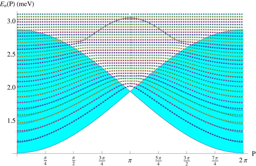
Figure 3: The same spectra as in Fig. 2 with added asymptotical curves explained in the text.

Five curves in the bottom display the spectra of five lightest modes calculated from the low-energy expansion (29). This expansion does not hold outside the filled region. The curve crossing the Zeeman ladder in the top of Fig. 3 represents the kinetic bound-state mode determined from (35). It is clear, however, that this are in fact the avoided crossings with exponentially narrow gaps.

Note, that all above asymptotical formulas cannot be used in the crossover region near the upper bound of the filled area.

4 Dynamical correlation function

Besides the magnetic excitation energy spectra, the inelastic neutron scattering allows one to measure the dynamical correlation function [1, 17]

$$S^{xx}(P,\omega)=S^{yy}(P,\omega)=\sum_{n=1}^{\infty}|\langle\Phi_{n}(P)|S_{0}^{x}|0\rangle|^{2}\,\delta[\omega-E_{n}(P)],$$ (36)

where $|0\rangle=|\ldots\uparrow\uparrow\uparrow\ldots\rangle$ is the ferromagnetic ground state, $S_{j}^{x}=\sigma_{j}^{x}/2$ is the $x$-spin operator at the site $j$, and the sum extends over all eigenstates of the Hamiltonian with the momentum $P$. Since the operator $S_{j}^{x}$ inverts just one spin at the site $j$ in the chain, it maps the ferromagnetic vacuum into the two-kink state,

$$S_{j}^{x}|0\rangle\equiv S_{j}^{x}|\ldots\uparrow\uparrow\stackrel{{\scriptstyle j}}{{\uparrow}}\uparrow\uparrow\ldots\rangle=\frac{1}{2}\,|\ldots\uparrow\uparrow\stackrel{{\scriptstyle j}}{{\downarrow}}\uparrow\uparrow\ldots\rangle\equiv\frac{1}{2}\,|j,1\rangle.$$

Accordingly, the dynamical correlation function (36) for model (3) takes the form

$$S^{xx}(P,\omega)=\frac{1}{4}\sum_{n=1}^{\infty}I_{n}(P)\,\delta[\omega-E_{n}(P)],$$ (37)

$$\sum_{n=1}^{\infty}I_{n}(P)=1,$$

where $I_{n}(P)$ is the relative intensity of the $n$-th mode,

$$I_{n}(P)=\frac{|\psi_{n}(l=1,P)|^{2}}{\sum_{l=1}^{\infty}|\psi_{n}(l,P)|^{2}}.$$ (38)

and $\psi_{n}(l,P)$ are the eigenfunctions of Hamiltonian (7).

Equations (36)-(38) are written in the assumption that Hamiltonian (3) has only the discrete spectrum. These relations can be easily modified in the case $h_{z}=0$, where the continuous spectrum exists:

$$S^{xx}(P,\omega)=\frac{1}{4}I_{kin}(P)\,\delta[\omega-E_{kin}(P)]+\frac{1}{2\pi}\int_{0}^{\pi}\rmd k\,I(k,P)\,\delta[\omega-E(k,P)],$$ (39)

$$I_{kin}(P)+\frac{2}{\pi}\int_{0}^{\pi}\rmd k\,I(k,P)=1,$$

where

$$I_{kin}(P)=\left\{\begin{array}[]{ll}0,&{\rm if}\quad|a|\leq 1\\ 1-a^{-2},&{\rm if}\quad|a|>1,\end{array}\right.$$ (42)

$$I(k,P)=\sin^{2}\gamma=\frac{\sin^{2}k}{1+2a\cos k+a^{2}},$$ (43)

and parameters $a$ and $\gamma$ are given by (15) and (12), respectively.

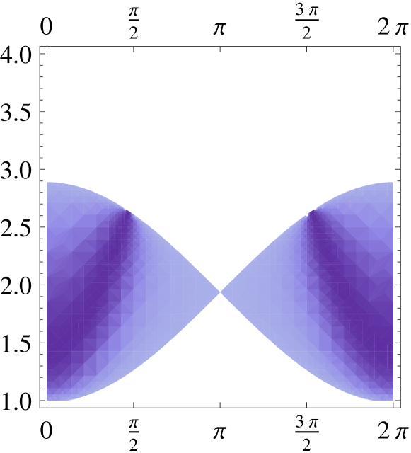
Figure 4: Intensity $I(k,P)$ of the continuous modes at $h_{z}=0$ in the $(P,E)$-plane determined from (43), (12). Darker regions correspond to larger intensity.

Fig. 4 displays the density plot of the intensity $I(k,P)$ of the continuous modes at $h_{z}=0$ in the $(P,E)$-plane determined from (43), (12) for the values of the rest parameter given by (26).

Formulae (36)-(38) can be directly used at nonzero longitudinal magnetic field $h_{z}>0$, since the spectrum is discrete in this case. Using the results of B, the relative intensities of the discrete modes can be expressed in terms of the Bessel function

$$I_{n}(P)=2\mu\left\{\frac{\partial}{\partial\nu}\left[\frac{J_{\nu}(1/\mu)}{J_{\nu+1}(1/\mu)}\right]\right\}^{-1}\bigg{|}_{\nu\to\nu_{n}},$$ (44)

where $\mu$ is given by (15), and $\nu_{n}$ is the $n$-th solution of equation (23).

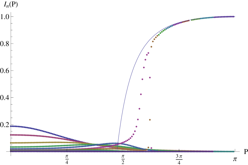
Figure 5: Intensities of the discrete modes $I_{n}(P)$ at a weak longitudinal magnetic field according to (44), with the parameter values (26). The solid curve represents the intensity $I_{kin}(P)$ of the kinetic mode at $h_{z}=0$, according to (42).

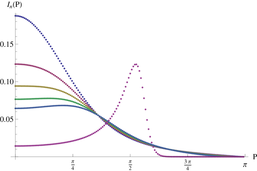
Figure 6: Intensities $I_{n}(P)$ for modes with $n=1,2,3,4,5,18$ at nonzero $h$ according to (44), (15), (26). Intensities $I_{n}(0)$ decrease with increase $n$.

Figures 5 and 6 show intensities $I_{n}(P)$ of discrete modes calculated from (44), (15) with the parameter values (26). Intensities $I_{n}(0)$ decrease with increasing $n$. Intensities of 30 lightest modes are plotted versus the momentum $P$ in Fig. 5, and those for $n=1,2,3,4,5,18$ are shown in Fig. 6. The intensity of the kinetic mode $I_{kin}(P)$ at $h_{z}=0$ is shown in Fig. 5 by the solid curve.

The obtained results are summarized in Fig. 7. It shows the same energy spectra as those in Fig. 2. The dispersion curves were calculated by use of equations (24)-(26). The darkness of the dispersion curves in Fig. 7 characterizes the relative intensities (44) for the corresponding modes. This figure looks quite similar to Fig. 3B of ref. [1], which displays the experimentally observed neutron scattering spectra in $\mathrm{Co}\mathrm{Nb}_{2}\mathrm{O}_{6}$.

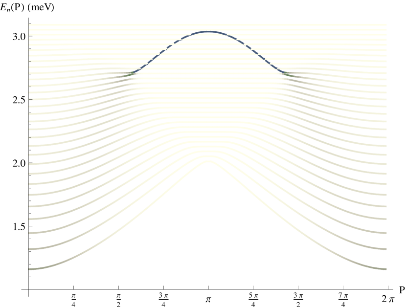
Figure 7: Energy spectra of 30 lowest modes according to (24), (25), (26). Darkness of the curves characterizes the intensities (44) of the modes.

5 Conclusions

In this paper we obtain the exact solution of the phenomenological model, which was proposed by Coldea et al[17] to describe the spectra of two-kink bound states in the entire Brillouin zone observed in the quasi-1D Ising ferromagnet $\mathrm{Co}\mathrm{Nb}_{2}\mathrm{O}_{6}$ in the inelastic neutron scattering experiments [1]. The model Hamiltonian acts in the space of two-kink configurations of the spin chain, and parametrizes hoppings of kinks along the chain, their short range interaction, and the linear long-range attracting potential leading to confinement of kink into pairs. We express the dispersion law $E_{n}(P)$ of two-kink bound states and relative neutron scattering intensities $I_{n}(P)$ by the magnetic modes in terms of the Bessel function. The preliminary analysis shows [18], that the obtained spectra $E_{n}(P)$ plotted in Fig. 2 display a good quantitative agreement with the experimental data. It would be interesting to perform the detailed comparison of obtained exact solutions [both for energies $E_{n}(P)$ and intensities $I_{n}(P)$] with the neutron scattering data in $\mathrm{Co}\mathrm{Nb}_{2}\mathrm{O}_{6}$.

Let us note, that the dispersionless modes forming the almost equidistant ladder with energies (34) and momenta near the zone boundary have very small intensities $I_{n}(P)$, as it is seen from Fig. 7. The reason is quite simple. It is well known, that the linear potential causes localization of a sole kink in the discrete spin chain, similarly to localization of an electron in the isolated conducting zone by the uniform electric field [19]. The dispersionless modes (34) correspond to large enough clusters of down-spins bounded by two well separated localized kinks, which can be hardly excited in the up-spin ground state by the neutrons scattering. Perhaps, such modes could be effectively excited by application of the oscillating magnetic field having the resonant frequency $\omega=h_{z}/\hbar$.

Appendix A Solution of the eigenvalue problem

In this Appendix we describe the exact solution of the eigenvalue problem (14), which we rewrite as

$$\left(-\lambda+\mu\,l+\frac{a\,\delta_{l,1}}{2}\right)\psi(l)-\frac{\psi(l+1)+\psi(l-1)}{2}=0,\quad\quad l=1,2,\ldots,$$ (45)

with the Dirichlet boundary conditions

$$\lim_{l\to+\infty}\psi(l)=0,$$ (46)

$$\psi(0)=0.$$ (47)

The following normalization condition for the eigenstate $\psi(l)$ will be chosen:

$$\psi(1)=-2.$$ (48)

Let us skip for a while the boundary condition (47) and consider the generating function $g(z)$ for $\psi(l)$,

$$g(z)=\sum_{l=1}^{\infty}\psi(l)\,z^{l}.$$ (49)

This function should be analytical inside the circle $|z|<1$, subject to the boundary condition

$$g(0)=0,$$ (50)

and satisfy the differential equation

$$[\epsilon(z)-\lambda]g(z)+\mu\,z\frac{dg(z)}{dz}=V(z),$$ (51)

following directly from (45), (48), (49). Here $\epsilon(z)$ is given by (19), and

$$V(z)=1+z\left[a+\frac{\psi(0)}{2}\right].$$ (52)

The solution of equation (51) satisfying (50) reads as

$$g(z)=\int_{0}^{z}\frac{\rmd z^{\prime}}{\mu z^{\prime}}\,V(z^{\prime})\exp\left\{\frac{\rmi}{\mu}[{\mathcal{F}}(z^{\prime})-{\mathcal{F}}(z)]\right\},$$ (53)

where

$$\rmi\,{\mathcal{F}}(z)=-\lambda\log z-\frac{1}{2}(z-z^{-1}),$$ (54)

and the branch of the logarithm is fixed by the condition ${\mathcal{F}}(1)=0$.

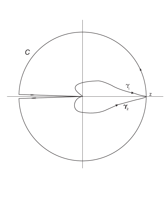
Figure 8: Integration paths in the $z^{\prime}$-plane: arcs $\gamma_{1}$ and $\gamma_{2}$ connecting the points $z^{\prime}=0$ and $z^{\prime}=z$ are the allowed integration paths in (53); loop $C$ is the integration path in (55).

At positive $\mu$, the integration path in the $z^{\prime}$-plane in (53) should approach the origin $z^{\prime}=0$ from the left half-plane ${\mathrm{R}e}\,z^{\prime}<0$ to provide convergence of the integral. Figure 8 shows two allowed integration paths $\gamma_{1}$ and $\gamma_{2}$ in the right-hand side of (53) for the case $z>0$. Integration along each of them should give the same function $g(z)$. This requirement leads to the following constraint (cf. equations (56), (57) in ref. [16])

$$\int_{C}\frac{\rmd z^{\prime}}{z^{\prime}}\,V(z^{\prime})\exp\left\{\frac{\rmi}{\mu}[{\mathcal{F}}(z^{\prime})]\right\}=0,$$ (55)

where the integration path $C=\gamma_{2}-\gamma_{1}$ is shown in Figure 8. Substitution of (52) into (55) gives the constant $\psi(0)$:

$$\psi(0)=-2\left[a+\frac{J_{\nu}(\mu^{-1})}{J_{\nu+1}(\mu^{-1})}\right],$$ (56)

where $\nu=-\lambda/\mu$, and $J_{\nu}(x)$ is the Bessel function. We have taken into account the integral representation of the Bessel function

$$J_{\alpha}(x)=\int_{C}\frac{\rmd z}{2\pi\rmi\,z}\,z^{\alpha}\exp[x(z^{-1}-z)/2],$$

which reduces to the well known form (see formula (5) in page 15 in [20]) after the change of the integration variable $z=1/u$.

Application of the Dirichlet boundary condition (47) leads then to the equation

$$J_{\nu}(\mu^{-1})+a\,J_{{\nu}+1}(\mu^{-1})=0,$$ (57)

which solutions $\nu_{n}$ determine the spectrum $\lambda_{n}=-\mu\,\nu_{n}$ of the problem (45)-(47).

Fig. 9 shows the plot of the left-hand side of equation (57) versus $\nu$ at $a=-0.5$, $\mu=0.05$.

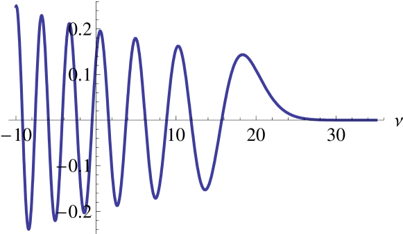
Figure 9: Plot of the function $J_{\nu}(\mu^{-1})+a\,J_{{\nu}+1}(\mu^{-1})$ versus $\nu$ at $a=-0.5$, $\mu=0.05$.

Appendix B Relative intensities of discrete modes at $\mu>0$

In this Appendix we prove the following
Statement.
Let the set of real numbers $\{\psi(l,\lambda)\}_{l=0}^{\infty}$ solves the linear problem

$$\left(-\lambda+\mu\,l+\frac{a\,\delta_{l,1}}{2}\right)\psi(l,\lambda)-\frac{\psi(l+1,\lambda)+\psi(l-1,\lambda)}{2}=0,\quad\quad l=1,2,\ldots,$$ (58)

with the boundary condition

$$\lim_{l\to+\infty}\psi(l,\lambda)=0.$$ (59)

Coefficients $a,\lambda,\mu$ are supposed to be real, and $\mu>0$.
Let us define the intensity $I(\lambda)$ corresponding to this solution as

$$I(\lambda)=\frac{[\psi(1,\lambda)]^{2}}{\sum_{l=1}^{\infty}[\psi(l,\lambda)]^{2}}.$$ (60)

Then

$$I(\lambda)=2\mu\left[\frac{\partial}{\partial\nu}\frac{J_{\nu}(\mu^{-1})}{J_{\nu+1}(\mu^{-1})}\right]^{-1}\Bigg{|}_{\nu=-\lambda/\mu}.$$ (61)

Proof.
Since definition (60) of $I(\lambda)$ does not depend on the normalization of the set $\{\psi(l,\lambda)\}_{l=0}^{\infty}$, we shall fix the latter by the condition

$$\psi(1,\lambda)=-2,$$ (62)

without loss of generality. Consider the solution $\{\psi(l,\lambda^{\prime})\}_{l=0}^{\infty}$ of the problem (58), (59), (62) in which $\lambda$ is replaced by $\lambda^{\prime}$. In particular, instead of (58) we get

$$\left(-\lambda^{\prime}+\mu\,l+\frac{a\,\delta_{l,1}}{2}\right)\psi(l,\lambda^{\prime})-\frac{\psi(l+1,\lambda^{\prime})+\psi^{\prime}(l-1,\lambda^{\prime})}{2}=0,\quad\quad l=1,2,\ldots$$ (63)

Let us multiply equation (58) by $\psi(l,\lambda^{\prime})$, and equation (63) by $\psi(l,\lambda)$, then subtract one equation from the another and sum the result over all natural $l$. As the result, we obtain

$$(\lambda^{\prime}-\lambda)\sum_{l=1}^{+\infty}\psi(l,\lambda)\,\psi(l,\lambda^{\prime})=\frac{1}{2}\left[\psi(1,\lambda^{\prime})\psi(0,\lambda)-\psi(1,\lambda)\psi(0,\lambda^{\prime})\right],$$ (64)

or

$$\sum_{l=1}^{+\infty}\psi(l,\lambda)\,\psi(l,\lambda^{\prime})=\frac{1}{2(\lambda^{\prime}-\lambda)}\left[\psi(1,\lambda^{\prime})\psi(0,\lambda)-\psi(1,\lambda)\psi(0,\lambda^{\prime})\right].$$ (65)

Taking into account the chosen normalization condition $\psi(1,\lambda)=\psi(1,\lambda^{\prime})=-2$, and proceeding in (65) to the limit $\lambda^{\prime}\to\lambda$, we get

$$\sum_{l=1}^{+\infty}[\psi(l,\lambda)]^{2}=\frac{d\psi(0,\lambda)}{d\lambda}.$$ (66)

Combining (66) with (56) yields

$$\sum_{l=1}^{+\infty}[\psi(l,\lambda)]^{2}=\frac{2}{\mu}\,\left[\frac{\partial}{\partial\nu}\frac{J_{\nu}(\mu^{-1})}{J_{\nu+1}(\mu^{-1})}\right]\Bigg{|}_{\nu=-\lambda/\mu}.$$ (67)

Substitution of (62) and (67) into (60) leads finally to the result (61).

References

References

- [1] R. Coldea, D. A. Tennant, E. M. Wheeler, E. Wawrzynska, D. Prabhakaran, M. Telling, K. Habicht, P. Smeibidl, and K. Kiefer. Quantum criticality in an Ising chain: Experimental evidence for emergent symmetry. Science, 327(5962):177–180, 2010.
- [2] S. Sachdev. Quantum Phase Transitions. Cambridge University Press, Cambridge, 1999.
- [3] B. M. McCoy and T. T. Wu. Two dimensional Ising field theory in a magnetic field: Breakup of the cut in the two-point function. Phys. Rev. D, 18(4):1259–1267, 1978.
- [4] A. B. Zamolodchikov. Integrals of motion and -matrix of the (scaled) Ising model with magnetic field. Int. J. Mod. Phys. A, 4(16):4235–4248, 1989.
- [5] G. Delfino, G. Mussardo, and P. Simonetti. Non-integrable quantum field theories as perturbations of certain integrable models. Nucl. Phys. B, 473(3):469–508, 1996. (Preprint hep-th/9603011).
- [6] G. Delfino and G. Mussardo. Non-integrable aspects of the multi-frequency Sine-Gordon model. Nucl. Phys. B, 516:675–703, 1998. (Preprint hep-th/9709028).
- [7] P. Fonseca and A. B. Zamolodchikov. Ising field theory in a magnetic field: Analytic properties of the free energy. J. Stat. Phys., 110(3-6):527–590, 2003. (Preprint hep-th/0112167).
- [8] P. Fonseca and A. B. Zamolodchikov. Ising spectroscopy : Mesons at , 2006. Preprint hep-th/0612304.
- [9] G. Delfino and P. Grinza. Confinement in the -state Potts field theory. Nucl. Phys. B, 791:265–283, 2008. (Preprint arXiv:0706.1020 ).
- [10] L. Lepori, G. Zs. Tóth, and G. Delfino. Particle spectrum of the -state Potts field theory: a numerical study. J. Stat. Mech., P11007, 2009. (Preprint arXiv:hep-th/0909.2192).
- [11] S. B. Rutkevich. Formfactor perturbation expansions and confinement in the Ising field theory. J. Phys. A, 131(5):917–939, June 2009. (Preprint cond-mat:0901.1571 ).
- [12] G. Mussardo. Statistical Field Theory: An Introduction to Exactly Solved Models in Statistical Physics. Oxford University Press, Oxford, 2010.
- [13] S. T. Carr and A. M. Tsvelik. Spectrum and correlation functions of a quasi-one-dimensional quantum Ising model. Phys. Rev. Lett., 90(17):177206, 2003. (Preprint arXiv:cond-mat/0212248).
- [14] M. J. Bhaseen and A. M. Tsvelik. Aspects of confinement in low dimensions, 2004. Preprint cond-mat/0409602.
- [15] S. B. Rutkevich. Two-kink bound states in the magnetically perturbed Potts field theory at , 2009. Preprint arXiv:cond-mat/0907.3671.
- [16] S. B. Rutkevich. Energy spectrum of bound-spinons in the quantum Ising spin-chain ferromagnet. J. Stat. Phys., 131(5):917–939, June 2008. (Preprint arXiv:0712.3189v1).
- [17] R. Coldea, D. A. Tennant, E. M. Wheeler, E. Wawrzynska, D. Prabhakaran, M. Telling, K. Habicht, P. Smeibidl, and K. Kiefer. Supporting online material for [1], 2010. www.sciencemag.org/cgi/content/full/327/5962/177/DC1.
- [18] R. Coldea. Private communication, 2010.
- [19] J. M. Ziman. Principles of the Theory of Solids. University Press, Cambridge, 1972.
- [20] H. Bateman. Higher Transcendental Functions, Volume II. McGraw-Hill, New York, 1953.