Bootstrap Percolation on Complex Networks

Abstract

We consider bootstrap percolation on uncorrelated complex networks. We obtain the phase diagram for this process with respect to two parameters: $f$, the fraction of vertices initially activated, and $p$, the fraction of undamaged vertices in the graph. We observe two transitions: the giant active component appears continuously at a first threshold. There may also be a second, discontinuous, hybrid transition at a higher threshold. Avalanches of activations increase in size as this second critical point is approached, finally diverging at this threshold. We describe the existence of a special critical point at which this second transition first appears. In networks with degree distributions whose second moment diverges (but whose first moment does not), we find a qualitatively different behavior. In this case the giant active component appears for any $f>0$ and $p>0$, and the discontinuous transition is absent. This means that the giant active component is robust to damage, and also is very easily activated. We also formulate a generalized bootstrap process in which each vertex can have an arbitrary threshold.

I Introduction

Bootstrap percolation serves as a useful model to describe in detail or in analogy a growing list of complex phenomena, including neuronal activity Eckmann et al. (2007); Soriano et al. (2008); Goltsev et al. (2009), jamming and rigidity transitions and glassy dynamics Sellitto et al. (2005); Toninelli et al. (2006), and magnetic systems Sabhapandit et al. (2002). Chalupa et al. Chalupa et al. (1979) introduced bootstrap percolation in a particular cellular automaton used to study some magnetic systems (for other applications see Ref. Sellitto et al. (2005)), see also the even earlier work of Pollak and Riess Pollak and Riess (1975). The standard bootstrap percolation process on a lattice operates as follows: sites are either active or inactive. Each site is initially active with a given probability $f$. Sites become active if $k$ nearest neighbors are active (with $k=2,3,...$). In the final state of the process, the fraction $\mathcal{S}_{\text{a}}(f)$ of all sites are active. Remarkably, the function $\mathcal{S}_{\text{a}}(f)$ may be discontinuous. It may have a jump at a bootstrap percolation threshold $f_{\text{c2}}$. We will see below that when this process takes place on a network, this is not the only threshold in this system.

Bootstrap percolation has been thoroughly studied on two and three dimensional lattices (see Holroyd (2003, 2006); Balogh and Bollobas (2006); Cerf and Cirillo (1999) and references therein). The existence of a sharp metastability threshold for bootstrap percolation in two-dimensional lattices was proved by Holroyd Holroyd (2003), and later generalized to $d$-dimensional lattices Holroyd (2006); Balogh and Bollobas (2006). More recently, bootstrap percolation has been studied on the random regular graph Balogh and Pittel (2007); Fontes and Schonmann (2008), and also on infinite trees Peres and Pete (2006). Finite random graphs have also been studied Whitney (2009). Watts proposed a model of opinions in social networks in which the thresholds at each vertex is a certain fraction of the neighbors, rather than an absolute number Watts (2002). Bootstrap percolation is closely related to another well known problem in graph theory, that of the $k$-core of random graphs Bollobas (1984); Pittel et al. (1996); Fernholz and Ramachandran (2004); Dorogovtsev et al. (2006a). The $k$-core of a graph is the maximal subgraph for which all vertices have at least $k$ neighbors within the $k$-core. It is important to note the difference between the stationary state of bootstrap percolation and the $k$-core. Bootstrap percolation is an activation process which starts from a subset of seed vertices and spreads over a network according to the activation rules described above. The $k$-core of the network can be found as an asymptotic structure obtained by a subsequent pruning of vertices which have less than $k$ neighbors. While the $k$-core has been extensively studied, there are no analytical investigations of bootstrap percolation on complex networks.

In this paper we describe bootstrap percolation on an arbitrary sparse, undirected, uncorrelated complex network of infinite size. Specifically, we use the configuration model (a random graph with a given degree sequence). We show that there are two types of critical phenomena: a continuous transition corresponding to the appearance of the giant active component, and a second, discontinuous, hybrid phase transition combining a jump and a singularity. (This transition is also often called “mixed”.) We show that network inhomogeneity strongly influences the critical behavior at the appearance of the giant active component in networks with divergent second and third moments and finite first moment of the degree distribution. In contrast, the hybrid phase transition has the same critical singularities for any network with finite second moment of the degree distribution. This second transition can be understood by considering the “subcritical” clusters of the network, consisting of vertices whose number of active neighbors is one less than the threshold. We show that these subcritical clusters give rise to avalanches of activations which become increasingly large as the threshold is approached. We also describe how the behavior changes when the network is damaged. The damaging here is the uniformly random removal of vertices, so that a fraction $p$ of vertices in a network are retained. We give the phase diagram showing the thresholds with respect to both the extent of damage to the network, and to the size of the initial seed group. In particular, there is a special critical threshold $p_{s}$ at which the discontinuous transition first appears. We also show that network topology can have a dramatic effect, as on so called scale-free networks with finite mean but divergent second moment of the degree distribution a qualitatively different behavior occurs. There is no phase transition in the $p$–$f$ plane, but instead a giant active component appears at any $f\,{>}\,0$ and is robust to any amount of damage ($p>0$). Finally, we generalize bootstrap percolation by considering a distribution of threshold values, so that each vertex may have its own threshold value. We briefly outline the equations for the active fraction of the network and the size of the giant active component in this general formulation, and show how the classical percolation problem and the usual bootstrap percolation (which we analyze in the remainder of this paper) are limiting cases.

II Results

Consider an arbitrary, sparse, uncorrelated complex random network in the infinite size limit. The structure of this network is completely determined by its degree distribution $P(q)$. An important (and convenient for analytical treatment) feature of this architecture is local tree-likeness, which means that finite loops can be neglected. For the time being we assume there are no vertices with degree zero. We denote by $\langle q\rangle$ the mean of the degree distribution and similarly $\langle q^{2}\rangle$ is the second moment. The network may also be damaged by the uniformly random removal of vertices so that a fraction $p$ of all original vertices remaining.

Vertices have either an “active” or an “inactive” state. Once activated, a vertex remains active. With probability $f$ each vertex is part of the seed group, and is in an active state from the start. The remaining vertices, (a fraction $1-f$) become active only if they have at least $k$ active neighbors. We iteratively activate vertices that meet this criterion until a steady state is reached.

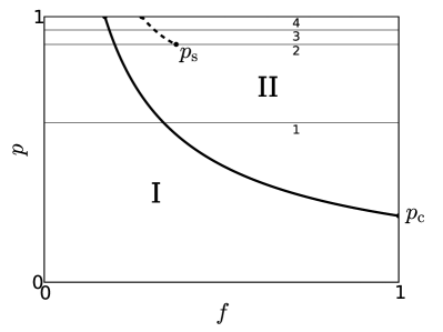
Figure 1: Phase diagram of bootstrap percolation in the $f$–$p$ plane for networks with finite second moment of the degree distribution, for $k\geq 2$ and smaller than an upper limit $k_{\text{max}}$ determined by the degree distribution. The solid line marks $f_{c1}$, the continuous appearance of the giant active component from $0$. The giant component of active vertices is present above this line in the upper-right portion of the diagram (labelled II) and absent in the area to the lower-left (I). The dashed heavy curve represents the discontinuous transition, $f_{c2}$. This line ends at the special critical point $p_{s}$. Thin horizontal lines show the location of the traces in Fig. 2 relative to the phase diagram features.

We define $\mathcal{S}_{\text{a}}$ to be the fraction of the vertices in the graph which are active at equilibrium (that is, including all active vertices, even those forming finite clusters), which is also the probability that an arbitrarily selected vertex is active in the final state of the bootstrap percolation process, and the size of the giant active component to be $\mathcal{S}_{\text{gc}}$, equal to the probability that an arbitrarily selected vertex belongs to the giant active component. By giant active component we mean a subgraph of active vertices which forms a connected component that occupies a finite fraction of the network.

In Fig. 1 we show a representative phase diagram for the giant active component in the $f$–$p$ plane for an uncorrelated infinite complex network whose degree distribution has finite second and third moments. Results are qualitatively the same for any such network. The giant active component is absent in the region labelled I, and present in the region labelled II. We see that if the network is sufficiently damaged so that the proportion of remaining vertices is less than a critical threshold $p_{\text{c}}$, the giant active component never appears, for any number of seed vertices. Above $p_{\text{c}}=\langle q\rangle/[\langle q^{2}\rangle-\langle q\rangle]$, which is equal to the well known percolation threshold (see, for example Dorogovtsev et al. (2008)),the giant active component appears at some value of $f$, $f_{\text{c1}}$, for a given value of $p$. This threshold is marked by the solid heavy line in the figure. This threshold is above zero for all $p>p_{\text{c}}$. In the limit $k\to\infty$ the boundary between regions I and II tends to the line $pf=p_{c}$, as the seed vertices may form a giant component in the graph. For large values of $p$, above a special critical point $p_{\text{s}}$, we discover a second transition in the size of the giant active component. For a given $p>p_{\text{s}}$ there is a threshold $f_{\text{c2}}>f_{\text{c1}}$ at which the size of the giant active component (and also the active fraction) jumps suddenly. These points are marked by the heavy dashed line in Fig. 1. Note that Fontes and Schonmann Fontes and Schonmann (2008) noticed on undamaged regular random graphs the two transitions we observe in more complex networks.

Figure 2: Probability that an arbitrarily chosen vertex is (a) active and (b) in a giant connected component of active vertices for an Erdős-Rényi graph of mean degree $5$, with $k=3$. The four lines (labelled from 1 to 4) are: $p=\{0.7,0.893,0.93,1\}$, corresponding to the relative positions in the phase diagram shown as thin horizontal lines in Fig. 1, namely: 1. $p_{\text{c}}<p<p_{\text{s}}$; 2. $p=p_{\text{s}}$; 3. $p_{\text{s}}<p<1$ and 4. $p=1$. The arrows in each plot mark the point of emergence ($f_{\text{c1}}$) of the giant active component for $p=1$. The small dot on each trace marks the point of the hybrid transition.

Fig. 2 shows the active fraction $\mathcal{S}_{\text{a}}$ and the size of the giant active component $\mathcal{S}_{\text{gc}}$ as a function of $f$ for four values of $p$ in an Erdős-Rényi graph (which has a Poisson degree distributions in the infinite size limit). We choose this network as it is representative of random graphs. For comparison, the position of each in the phase diagram is marked by a faint solid line in Fig. 1. Line $1$ is for a value of $p$ before the appearance of the jump. Line $2$ is exactly at the special critical point $p_{\text{s}}$ at which the jump appears. Line $3$ is at a $p>p_{\text{s}}$ where there is a jump. The location of the jump moves to smaller values of $f$ as $p$ increases, but never reaches zero, as is demonstrated by line $4$, which is at $p=1$. The giant active component appears continuously and linearly from zero, exactly as it does in ordinary percolation Albert and Barabási (2002); Dorogovtsev and Mendes (2002); Dorogovtsev et al. (2008). It is interesting to note that there is no discontinuity in $\mathcal{S}_{\text{a}}$ at $f_{\text{c1}}$ (marked by a small arrow), i.e., the threshold is invisible (hidden) when observing only the overall activation of the network.

For $k=1$ the jump does not appear, we have only the continuous transition. For larger $k$ there is a jump, and it appears at larger values of $f$ (for a given $p$) the larger $k$ is. The value of $p_{s}$ also increases, such that there is a finite maximum threshold, $k_{\text{max}}$ (proportional to the mean degree of the network for Erdős-Rényi graphs) beyond which the jump no longer appears. That is, the dashed line in Fig. 1, which marks the location of the jump, moves to the right and towards the top of the graph as $k$ increases, finally disappearing completely above $k_{\text{max}}$. This discontinuous transition has a hybrid character, with both a discontinuity and a singularity: when approaching $f_{\text{c2}}$ from below the size of the giant active component approaches the value at the bottom of the jump as the square-root of the distance from $f_{\text{c2}}$:

$$\mathcal{S}_{\text{a}}(f)=\mathcal{S}_{\text{a}}(f_{\text{c2}})-a(f_{\text{c2}}-f)^{1/2},$$ (1)

where $a$ is a constant (see Section III below for the origin of this equation). Lines $3$ and $4$ in Fig. 2 illustrate this situation. The same result holds with respect to $p$ if we were to approach this jump along a line of constant $f$. The size of the giant active component, $\mathcal{S}_{\text{gc}}$, has the same critical behavior.

The height of the jump decreases with decreasing $p$ (while $f_{\text{c2}}$ increases slightly), disappearing at the special point $p_{\text{s}}$. (The line labelled $2$ in Fig. 2 is at $p=p_{\text{s}}$.) At this point the behavior is different, as the size of the giant component approaches $f_{\text{c2}}$ now as the cube-root of the distance from the threshold (see Section III):

$$\mathcal{S}_{\text{a}}=\mathcal{S}_{\text{a}}(f_{\text{c2}})-a^{\prime}(f_{\text{c2}}-f)^{1/3},$$ (2)

where $a^{\prime}$ is a constant.

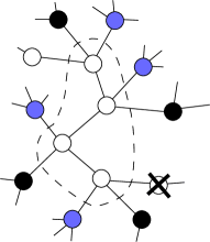
Figure 3: Left: A subcritical cluster in a network with threshold $k=3$. Filled black vertices are seed vertices, shaded vertices are active vertices while empty vertices are inactive. The vertices inside the dashed loop form a subcritical cluster, while those connected to them are either inactive or have more than the threshold number of active neighbors. If a single vertex neighboring a subcritical cluster becomes active (for example, if it became a seed vertex)—here marked by a cross —it’s neighbor inside the subcritical cluster must become active, and then it’s neighbors, until the entire cluster is activated, as shown on the right.

To understand the discontinuous “jump” in the size of the active component of the graph, we consider the subcritical clusters, a concept related to the corona clusters which were used to describe a similar transition in $k$-core percolation Goltsev et al. (2006); Dorogovtsev et al. (2006b); Schwarz et al. (2006). The subcritical vertices of the graph are the vertices whose number of active neighbors is precisely one less than the threshold of activation for that vertex. An example of a small subcritical cluster is illustrated in Fig. 3.

Clusters of subcritical vertices are important because of the following quality. The activation of even a single vertex neighboring the subcritical cluster necessarily leads to at least one of the members of the cluster now meeting its activation threshold. In turn, this will activate one of its neighbors in the cluster, and so on, so that an avalanche of activations ensues until the entire subcritical cluster becomes active—see Fig. 3. Below and above the jump, the subcritical vertices form only finite and isolated clusters, but as $f_{\text{c2}}$ is approached from below, the mean size of the subcritical clusters diverges. Hence the avalanches resulting from the change in activation state of a single vertex form a finite fraction of the entire graph, leading to a discontinuous change in the size of the active fraction of the graph. This argument will be made more precisely in the analysis in Section IV below.

When the degree distribution of the network decays very slowly, specifically in networks with divergent second moment $\langle q^{2}\rangle$ or third moment $\langle q^{3}\rangle$ of the degree distribution, the results are different from those described above. In particular, this is the case if the degree distribution tends to the form $P(q)\propto q^{-\gamma}$ with $\gamma\leq 4$ for large $q$. If $\gamma\leq 2$ the mean of the degree distribution also diverges, but we do not consider this case here. If $2<\gamma\leq 3$, the second moment diverges. These scale-free networks are of particular interest because many large real natural and technological networks appear to be of this kind Albert and Barabási (2002); Dorogovtsev and Mendes (2002). In this case (in the limit $N\to\infty$) a finite fraction of vertices is activated at any $p$ or $f>0$, and for any arbitrary activation threshold $k$. In other words the location of the jump tends to zero as the size of the network increases—so in very large scale-free networks we will not find (at finite $f$ or $p$) either of the transitions observed in graphs with fast decaying degree distributions. This means that, as has been found in several other cases Albert et al. (2000); Cohen et al. (2000), such scale-free networks are very robust to damage, and also that such a network is very easily activated.

When $3<\gamma\leq 4$, the phase diagram is qualitatively the same as that shown in Fig. 1. The giant active component appears at finite $p$ ( or $f$) with a continuous transition. However, rather than growing linearly near the transition point, the size of the giant active component increases as the distance from the critical point raised to the power $1/(\gamma-3)$.

III Basic Analysis

In this section and the two following, we describe in more detail how the results already described may be obtained.

Consider choosing an arbitrary vertex from the network. We wish to calculate the probability $\mathcal{S}_{\text{a}}$ that this vertex is active in the equilibrium state. To calculate this probability, we first define $Z$ as follows: $Z$ is the probability that, on following an arbitrary edge in the graph, we reach a vertex which is either a seed vertex or has at least $k$ downstream neighbors that are active. (By downstream we mean neighbors of the vertex reached by the edges other than the one we arrived from.) To be active, these downstream neighbors in turn must fulfil this same condition, that they are either seed vertices or they have $k$ further downstream neighbors of their own that are previously active.

Table 1: Symbols used in graphical representations of self-consistency equation.

We can graphically represent this recursive relationship using the symbols given in Table 1. The probability $Z$ is represented by an edge ending in a square. A seed vertex is represented by a black disc, and other vertices by open discs. An edge crossed by a short line at its end represents the probability $1-Z$, that is the probability of encountering a vertex that doesn’t satisfy the condition for $Z$. Thus we obtain the following representation for $Z$:

The terms on the right hand side represent sums of the probabilities of all such terms. Based on this diagram, we write mathematical expressions for the probabilities represented by each of these symbols, allowing us to construct the following self-consistency equation for $Z$:

$$Z=pf+p(1-f)\sum_{i=k}^{\infty} \frac{(i+1)P(i+1)}{\langle q\rangle}$$

$$\times\sum_{l=k}^{i}\binom{i}{l}Z^{l}(1-Z)^{i-l}.$$ (3)

The probability $\mathcal{S}_{a}$, represented by a shaded disc, is the sum of two terms, as represented in this diagram:

The first is the probability that the vertex is active from the beginning ($pf$), the second [with prefactor $p(1-f)$] is the probability that it has at least $k$ neighbors that would be active even if the vertex we are observing was inactive. But each neighbor satisfies this condition precisely with probability $Z$, as represented by squares in the diagram. Converting to a mathematical expression, this gives the following equation:

$$\mathcal{S}_{\text{a}}=pf+p(1-f)\sum_{i=k}^{\infty}P(i)\sum_{l=k}^{i}\binom{i}{l}Z^{l}(1-Z)^{i-l}.$$ (4)

The probability $\mathcal{S}_{\text{gc}}$ that an arbitrarily chosen vertex belongs to the giant active component can be constructed in a similar way, but we must impose the further condition that a vertex has an edge leading to an active subtree of infinite extent. We define $X$ to be the probability that the vertex encountered upon following an arbitrarily chosen edge meets the conditions for $Z$ and also has an edge leading to an active subtree of infinite extent. Graphically, we represent the probability $X$ by an infinity symbol at the end of an edge, and a self-consistency condition for $X$ is expressed by the diagram:

This corresponds to the equation:

$$X=pf \sum_{i=0}^{\infty}\frac{(i+1)P(i+1)}{\langle q\rangle}\sum_{m=1}^{i}\binom{i}{m}X^{m}(1-X)^{i-m}$$

$$+ p(1-f)\sum_{i=k}^{\infty}\frac{(i+1)P(i+1)}{\langle q\rangle}\sum_{l=k}^{i}\binom{i}{l}$$

$${\times}\sum_{m=1}^{l}\binom{l}{m}X^{m}(Z-X)^{l-m}(1-Z)^{i-l}.$$ (5)

The probability $\mathcal{S}_{gc}$ (the probability that an arbitrary vertex belongs to a giant active component, represented below by a shaded circle containing the infinity symbol—see Table 1) is the sum of the probability that the vertex is a seed vertex that is connected to an infinite active subtree (probability $X$) and of the probability that the vertex is not a seed vertex but has at least $k$ independently active neighbors (probability $Z$), at least one of which also leads to an infinite active subtree. Thus

so that, similarly to Eq. (4), we can write $\mathcal{S}_{\text{gc}}$ in terms of $X$ and $Z$:

$$\mathcal{S}_{\text{gc}}= pf\sum_{i=0}^{\infty}P(i)\sum_{m=1}^{i}X^{m}(1-X)^{i-m}$$

$$+p(1-f)\sum_{i=k}^{\infty}P(i)\sum_{l=k}^{i}\binom{i}{l}$$

$$\times\sum_{m=1}^{l}\binom{l}{m}X^{m}(Z-X)^{l-m}(1-Z)^{i-l}.$$ (6)

It will be useful to define $\Psi(Z,p,f)$ to be the right-hand side of Eq. (3), and $\Phi(X,Z,p,f)$ the right-hand side of Eq. (5), so that these two equations become

$$Z=\Psi(Z,p,f),$$ (7)

and

$$X=\Phi(X,Z,p,f).$$ (8)

These equations can be solved numerically for a given network degree distribution. If multiple solutions exist, the physical solution for $Z$ is always the smallest value. The location, $f_{c1}$ of the appearance of the giant active component can be found by assuming $X$ is small but non-zero in Eq. (8), taking the limit as $X$ tends to zero and solving for $f$ for a given $p$ (or vice versa). In this way we also find that $X$ and hence $\mathcal{S}_{\text{gc}}$ grow linearly from the critical point $f_{c1}$ for networks with $\langle q^{2}\rangle$ finite. The results mentioned below also correspond to this case—we will examine the case $\langle q^{2}\rangle\to\infty$ subsequently.

The second, discontinuous, transition can be located by observing that the jump occurs when, (after a second solution appears) the smallest $Z$ solution of Eq. (7) disappears. At this point $\Psi(Z)$ just coincides with the value of $Z$, and a little consideration reveals that this must be at a local extremum of $\Psi/Z$. Thus the discontinuous transition can be found by simultaneously solving Eq. (7) and

$$\frac{d}{dZ}\left(\frac{\Psi}{Z}\right)=0$$ (9)

for $f$. The fact that the first derivative vanishes leads to the square-root scaling near the critical point, with respect to either $f$ or $p$—see Eq. (1). The jump disappears at a special critical point $p_{\text{s}}$ in the $f-p$ plane which satisfies Eqs. (3), (9) and a third condition

$$\frac{d^{2}}{dZ^{2}}\left(\frac{\Psi}{Z}\right)=0.$$ (10)

This condition means that the scaling below $p_{s}$ (see Fig. 1) is cube-root—see Eq. (2).

IV Avalanches

The singular behavior [Eq. (1)] near the hybrid transition can be understood by considering the subcritical clusters of the active subgraph. These form a subset of the inactive portion of the graph consisting only of those vertices whose number of active neighbors is exactly one less than the activation threshold for that vertex—see Fig. 3. That is, the subcritical subgraph consists of all those vertices which are not seed vertices and which have exactly $k-1$ active neighbors. The subcritical clusters are finite everywhere except exactly at the point of the jump transition. To show that this is the case, we use a generating function approach, similar to that used in Goltsev et al. (2006); Callaway et al. (2000); Newman et al. (2001), to calculate $\langle s\rangle_{\text{sub}}$, the mean size of the subcritical clusters.

Let $F_{0}(x)$ be the generating function for the probability that an arbitrarily chosen vertex is subcritical. By considering the probability that an arbitrarily chosen vertex is subcritical, which corresponds to $F_{0}(1)$, we can write

$$F_{0}(x)= p(1-f)$$

$$\times\sum_{q\geq k-1}P(q)\binom{q}{k-1}Z^{k-1}(1-Z)^{q-k+1}x^{q-k+1}.$$ (11)

Similarly, the generating function for the probability that an arbitrarily chosen edge leads to a subcritical vertex is

$$F_{1}(x)=p(1-f)\sum_{q\geq k}\frac{qP(q)}{\langle q\rangle}\binom{q-1}{k-1}Z^{k-1}(1-Z)^{q-k}x^{q-k}.$$ (12)

The generating function for the probability that a randomly chosen vertex belongs to a subcritical cluster of a given size then must obey the self-consistency equation Callaway et al. (2000); Newman et al. (2001)

$$H_{0}(x)=1-F_{0}(1)+xF_{0}[H_{1}(x)],$$ (13)

where $1-F_{0}(1)$ represents the probability that the randomly chosen vertex is not itself subcritical, and the second term is a recursive relationship, ensuring that successive powers of $x$ correspond to the probabilities of encountering a cluster size matching that power. In this equation $H_{1}(x)$ is the related generating function for the probability that a subcritical cluster of a given size is reached upon following an arbitrarily chosen edge. In a similar way we can write a self-consistency equation for this:

$$H_{1}(x)=1-F_{1}(1)+xF_{1}[H_{1}(x)].$$ (14)

Where $1-F_{1}(1)$ is the probability that the arbitrarily chosen edge leads to a vertex that is not subcritical. Note that $H_{0}(1)=H_{1}(1)=1$.

From these generating functions, we can calculate various quantities related to the subcritical clusters. For example, the distribution of avalanche sizes (which are the same as the sizes of the subcritical clusters) is given by

$$G(s)=\frac{1}{s!}\frac{d^{s}H_{0}(x)}{dx^{s}}\bigg{|}_{x=0}$$ (15)

and we expect that at the critical point $G(s)\sim s^{-3/2}$. The mean size of the subcritical clusters is simply

$$\langle s\rangle_{\text{sub}}= \frac{dH_{0}}{dx}\bigg{|}_{x=1}$$

$$= F_{0}(1)+p(1-f)\sum_{q\geq k-1}P(q)\binom{q}{k-1}$$

$$\times Z^{k-1}(1-Z)^{q-k+1}(q-k+1)\frac{dH_{1}}{dx}\bigg{|}_{x=1}.$$ (16)

Using Eqs. (14), (12) and comparing with Eqs. (3) and (7) we find that

$$\frac{dH_{1}}{dx}\bigg{|}_{x=1}=\frac{F_{1}(1)}{1-d\Psi(Z)/dZ}.$$ (17)

Now from Eq. (9), $d\Psi(Z)/dZ=1$ at the critical point, and $1-d\Psi(Z)/dZ\propto Z-Z_{j}\propto(f_{\text{c2}}-f)^{1/2}$, near the critical point. Thus, near this point, therefore, the term containing $dH_{1}/dx\big{|}_{x=1}$dominates $\langle s\rangle_{\text{sub}}$ so that

$$\langle s\rangle_{\text{sub}}\propto(f_{\text{c2}}-f)^{-1/2},$$ (18)

or alternatively, for fixed $f$, $\langle s\rangle_{\text{sub}}\propto(p_{\text{c2}}-p)^{-1/2}$, hence the mean size of the corona clusters diverges at the critical point.

The addition of a single vertex (an infinitesimal increase in $p$) or activation of a seed vertex (increment of $f$) may lead to the activation of a subcritical vertex and hence activating an entire subcritical cluster in an avalanche. At $f_{\text{c2}}$, the subcritical clusters span the whole graph, so the activation of a vertex can lead to an avalanche of activation that eventually affects a finite fraction of the whole infinite graph hence we see a discontinuity in both the size of the active fraction and the giant active component. Note that for $f>f_{c2}$ the mean size of the subcritical clusters is finite.

V Scale-free graphs

Let us consider degree distributions that tend to $P(q)\propto q^{-\gamma}$ for large $q$ where exponent $\gamma$ is some positive constant usually $>2$. For concreteness, in the following we will consider the degree distribution

$$P(q)=Aq^{-\gamma}\qquad\mbox{ for }q\geq q_{0},$$ (19)

where $A$ is a constant of normalization. For $\gamma>4$ the results are qualitatively the same as those described above.

When $\gamma\leq 3$ the second moment of the degree distribution diverges, leading to different behavior. The results that follow refer to the situation when $2<\gamma\leq 3$. Note that many real world networks, especially biological networks have exponent in the range $1<\gamma\leq 2$ Albert and Barabási (2002); Dorogovtsev and Mendes (2002); Bonifazi et al. (2009). In this case the first moment also diverges. We don’t consider this case here.

By assuming $Z$ to be small, we can approximate $\Psi(Z)$ by considering only leading order in $Z$. Then the self consistency equation (3) becomes:

$$Z\approx p(1-f)aZ^{\gamma-2}+pf.$$ (20)

For $p>0$, this equation has no small-$Z$ solution, even in the limit $f\to 0$. Because the only solutions for $Z$ as $f\to 0$ are therefore of order $1$ it is clear that the discontinuous transition is moved to $f=0$ for scale-free graphs. A similar analysis for the giant active component—approximating $\Phi(Z,X)$ [the RHS of Eq. (5)] by assuming $X$ and $Z$ both small leads to similar conclusion about $X$: that there are no infinitesimal solutions in the limit $f\to 0$, confirming that there is no jump for $f>0$ but also that the giant active component appears for any $f>0$ and $p>0$.

To add support to this approximation, consider the same degree distribution as before, but truncated at some maximum degree $q_{\text{cut}}$ (the normalization constant will also necessarily change). If we re-derive (20) assuming a finite $q_{\text{cut}}$, we find

$$Z\approx p(1-f)bZ^{k}+pf$$ (21)

which does have a solution at finite $p$ (or $f$). For finite $q_{\text{cut}}$, numerical solution of Eq. (3) shows a jump appears at small values of $f$. As $q_{\text{cut}}$ is increased, the curve of this jump moves closer to $f=0$, and extends towards $p=0$. Similarly the giant component appears at smaller and smaller values of $p$ and $f$ as $q_{\text{cut}}$ is increased. In keeping with the approximate analysis just described, we expect that both thresholds reach $f=0$ and $p=0$ in the infinite size limit. In summary, when $2<\gamma\leq 3$, the giant active component is always present everywhere in the $p-f$ plane for $p>0$ and $f>0$, and appears not from zero but with a finite size.

When $3<\gamma\leq 4$, an expansion of the right-hand-side of Eq. (5) in leading powers of $X$ gives an equation of the form

$$X=c_{1}X+c_{2}X^{\gamma-2}+...\,,$$ (22)

where the ellipsis signifies further terms of higher order in $X$. The first coefficient $c_{1}=pf\frac{\langle q^{2}\rangle-\langle q\rangle}{\langle q\rangle}+p(1-f)B(Z)$, where $B(Z)$ is a function of the variable $Z$. Thus when $f<1$ the value of $c_{1}$ differs from that found in the percolation problem. The presence of a finite linear term ($c_{1}>0$) means that the appearance of the giant component occurs at non-zero values of $p$ (or $f$) – at a point which can be found by solving $c_{1}=1$. However, because the second leading exponent is $\gamma-2$ and not $2$, $X$ scales as $(p-p_{c1})^{\beta}$, near the appearance of the giant component, with $\beta=1/(\gamma-3)$. This is the same scaling as found in the usual percolation problem Cohen et al. (2002). Curiously, the second coefficient $c_{2}$ is simply equal to $p$ up to a factor depending on the degree distribution. Above $\gamma=4$, we find $\beta=1$ as found for the usual percolation.

VI General distribution of activation thresholds $k$

The bootstrap percolation process described above can be thought of as a specific case of a more general process in which the threshold values can be different for each vertex. Assuming no correlations between vertex degree and threshold value, we can define a distribution $Q(k)$ such that $Q(k)$ is the fraction of vertices which have threshold value $k$. The fraction of seed vertices is then $Q(0)$. Setting $Q(0)=f$ and $Q(k)=1-f$ for some $k\geq 2$ we recover the bootstrap percolation model described above.

In the general case, we find that the equation for the active fraction is

$$\mathcal{S}_{\text{a}}=p\sum_{k\geq 0}Q(k)\sum_{i=k}^{\infty}P(i)\left[\sum_{l=k}^{i}\binom{i}{l}Z^{l}(1-Z)^{i-l}\right],$$ (23)

where, as above, $Z$ is the probability of encountering a vertex with at least $k$ downstream active neighbors upon following an arbitrary edge:

$$Z=p\sum_{k\geq 0}Q(k)\sum_{i=k}^{\infty}\frac{(i+1)P(i+1)}{\langle q\rangle}\sum_{l=k}^{i}\binom{i}{l}Z^{l}(1-Z)^{i-l}.$$ (24)

These two equations are similar to those presented in Gleeson (2008) for undamaged networks as a generalization of the Watts model Watts (2002).

Similarly, the equation for the giant active component is

$$\mathcal{S}_{\text{gc}}=p\sum_{k\geq 0}Q(k) \sum_{i=k}^{\infty}P(i)\sum_{l=k}^{i}\binom{i}{l}$$

$$\times\sum_{m=1}^{l}\binom{l}{m}X^{m}(Z-X)^{l-m}(1-Z)^{i-l},$$ (25)

where as before $X$ is the probability that an edge leads to an infinite active subtree:

$$X= p\sum_{k\geq 0}Q(k)\sum_{i=k}^{\infty}\frac{(i+1)P(i+1)}{\langle q\rangle}$$

$${\times}\sum_{l=k}^{i}\binom{i}{l}\sum_{m=1}^{l}\binom{l}{m}X^{m}(Z-X)^{l-m}(1-Z)^{i-l}.$$ (26)

Vertices which have $k=1$ become active if they have a single active neighbor. Thus a single seed vertex will activate an entire connected cluster of such vertices. In particular, if there is a giant connected cluster in the network (i.e. if $p\geq p_{c}$, the percolation threshold), the introduction of a finite number of seed vertices into the infinite network will (almost surely) activate the giant connected component. In other words, we have behavior equivalent to ordinary percolation. In particular, if we set $Q(0)+Q(1)=1$ (and requiring that, if $Q(0)\to 0$, the number of seed vertices remains sufficient to activate the giant component of the network) then we recover from Eqs. (25) and (26) the well known percolation equations Dorogovtsev et al. (2008).

VII Discussion

In this paper we have extended the understanding of bootstrap percolation to uncorrelated infinite random graphs with arbitrary degree distribution, and studied the effects of damage to the network. We have found that the phase diagram for the giant active component with respect to damage to the network ($1-p$) and the fraction of initially active vertices ($f$) has several interesting features. There are two transitions observed. At the first the giant active component appears continuously from zero, and at the second (always at a higher initial activation fraction) there is a hybrid phase transition, where the size of the giant active component has a discontinuity—a ‘jump’—while also having a singularity, as the size of the giant active component approaches the transition from below as the square root of the distance from the critical point. This singular behavior is due to avalanches in the activation process. The sizes of avalanches of activation are determined by the size of subcritical clusters—clusters of vertices whose number of active neighbors is exactly one less than the activation threshold. Everywhere but at the hybrid transition these subcritical clusters are finite (though together occupying a finite fraction of the network), but as the transition is approached these clusters grow as the reciprocal of the square-root of the distance from the transition. We also observe a new special critical point, at the level of damage at which the second transition first appears. Here the height of the jump tends to zero, and the scaling near the critical point is the cube-root of the distance from the threshold. These results are valid for arbitrary degree distributions, so long as they decay rapidly enough that the second and third moments of the distribution are bounded. Note that we could express our results not in terms of $f$ and $p$, but of $f$ and any other convenient parameter, for example, the mean degree $\langle q\rangle$ of a network. This allows one to apply our conclusions to arbitrary uncorrelated networks.

Network inhomogeneity plays an important role. When the second moment of the degree distribution is bounded but the third moment is unbounded, the critical scaling near the appearance of the giant active component is not simply linear but has higher order scaling, depending on the degree distribution. When the second moment is unbounded, for example in scale-free networks with degree distribution exponent $\gamma\leq 3$, both thresholds tend to $f=0$ and $p=0$ in the infinite size limit. Thus the phase diagram is featureless, with a giant active component (albeit sometimes very small) present for any finite activation and any amount of damage to the network. This result has important implications for real world networks. For example, the network of neurons in the brain may have such a scale-free organization Sporns et al. (2004) meaning that brain activity may be able to be instigated with very small stimulus (even though such networks, whilst large, are of course finite).

In summary, we have obtained phase diagrams for the bootstrap percolation problem in a wide range of complex networks. We have described the properties and the nature of two distinct transitions in this problem: the bootstrap percolation transition and the emergence of a giant connected component (percolative cluster) of active vertices.