Uncertainty-principle noise in vacuum-tunneling transducers

Abstract

The fundamental sources of noise in a vacuum-tunneling probe used as an electromechanical transducer to monitor the location of a test mass are examined using a first-quantization formalism. We show that a tunneling transducer enforces the Heisenberg uncertainty principle for the position and momentum of a test mass monitored by the transducer through the presence of two sources of noise: the shot noise of the tunneling current and the momentum fluctuations transferred by the tunneling electrons to the test mass. We analyze a number of cases including symmetric and asymmetric rectangular potential barriers and a barrier in which there is a constant electric field. Practical configurations for reaching the quantum limit in measurements of the position of macroscopic bodies with such a class of transducers are studied.

I Introduction

The investigation of the ultimate quantum limits for the detection of weak forces has been stimulated by the development of sensitive antennae to search for gravitational wave radiation PRB1 ; PRB2 . If several practical barriers can be overcome and electromechanical transducers of sufficient sensitivity are developed, then it should be possible to monitor massive Weber-bar gravitational wave antennae in the regime in which their behavior is dominated by quantum effects, i.e., by the measurement process itself. Thus a class of experiments in which repeated measurements are performed on a single isolated macroscopic quantum-mechanical oscillator may become possible PRB3 ; PRB4 .

So far superconducting-quantum-interference-device (SQUID)-based electromechanical transducers have offered the best opportunity to study the quantum regime. However, recently it was pointed out that the tunneling probe used in the scanning tunneling microscope is a quantum limited electromechanical amplifier and therefore may present an opportunity to study the quantum regime with electromechanical transducers PRB5 .

Since the tunneling transducer is intrinsically a quantum device, without a classical analog, a quantum analysis is required to understand the origin of its noise. It was shown that there are two independent sources of noise in the tunneling transducer PRB6 ; PRB7 . The first is the well-known shot noise of the tunneling current which enters as an apparent fluctuation of the test mass. The other source of noise is a fluctuating “back-action” force which the tunneling transducer exerts on the test mass. The two sources of noise work in concert to add to the amplified mechanical signal an amount of noise power equivalent to one-half quantum of energy per second at the operating frequency. Recently Yurke and Kochanski presented a full quantum-mechanical analysis of the noise of a tunneling transducer PRB8 . They used a second-quantized description of electron tunneling through a barrier to find an expression for the uncertainty in the width of the tunneling barrier, which is equivalent to the position of the test mass, based upon the tunneling current fluctuations. They also computed the fluctuation of the momentum current transported across the barrier. Their calculations explicitly show that the tunneling transducer enforces the Heisenberg uncertainty relation between the position and momentum of the test mass.

The purpose of this paper is twofold. The first purpose is to present a simplified, first-quantization treatment of the noise in the tunneling transducer. Although we obtain the same expressions for the uncertainties as Yurke and Kochanski in Ref. 8, we think that the use of first quantization to deal with this problem is more physically intuitive and less mathematically complex. The second purpose of this paper is to discuss some of the practical considerations regarding the tunneling transducer and the prospects for achieving quantum noise limited force detection.

The paper is organized as follows. In Sec. II, after a brief description of the working principles of the tunneling transducer, we express the position and the momentum uncertainties in terms of the time-independent solutions of the Schrödinger equation. The position uncertainty is derived from the transmission coefficient and the momentum uncertainty is obtained by a generalization of the current flux. In Sec. III we apply these considerations to calculate the position and momentum uncertainty product for symmetric and asymmetric rectangular barriers. In Sec. IV we treat the case of a barrier in which there is a constant electric field. In Sec. V we discuss the practical obstacles to achieving quantum noise dominance and we give a specific example of a configuration in which quantum effects may be observed. In Sec. VI we discuss some conceptual problems in making the correspondence between the quantum mechanical uncertainties which are calculated here and the more experimentally relevant classical description of noise which employs spectral densities of random variables.

II Position and momentum uncertainties for a tunneling transducer

The tunneling transducer is simply a variable resistance transducer. The motion of a test mass modulates the gap of a vacuum tunnel junction thus affecting the tunneling probability. If the junction is voltage biased then the current measured by an amplifier which follows the tunnel probe provides a sensitive measure of the tunneling gap and therefore of the displacement of the test mass.

In Figure 1 we show a schematic representation of the tunneling transducer. A tunneling tip is places a distance $l$ from the test mass which is going to be monitored. The displacement of the test mass from its initial position is given by $x$. The effective resistance of the tunneling transducer is given, in the limit $k_{0}l\gg 1$, by the familiar formula

$$R=R_{0}e^{-2k_{0}x},$$ (1)

where $k_{0}$ is the inverse of the de Broglie wavelength of the electrons with energy $E$ inside the barrier of height $V_{0}$ and is given by

$$k_{0}=\left[\frac{2m(V_{0}-E)}{\hbar^{2}}\right]^{1/2}.$$ (2)

The tunneling resistance $R_{0}$ is usually around $10^{6}-10^{8}\Omega$ and a typical value of $k_{0}$ is $10^{10}$ m^-1; the distance scale over which the tunneling resistance change significantly is of atomic dimensions. For typical values of the tunnel probe voltage bias the tunneling current is in the range of nanoamps to microamps. Using conventional electronic techniques it is possible to measure extremely small fractional changes in currents of this magnitude so it is possible with the tunnel junction transducer to measure displacements which are a very small fraction of $k_{0}^{-1}$.

It is important that the capacitance between the tunneling probe and the test mass be small, on the order of $10^{-17}$ F or less PRB7 . This ensures that the quantum effects associated with the tunneling transducer will dominate the back-action force fluctuations that have their origin in the amplifier used to sense the tunneling current and which are capacitively coupled to the test mass. This assumption allows us to concentrate on the fluctuations which arise from the tunneling process.

We express the uncertainties in the position and the momentum of the test mass which is sensed by the tunneling transducer in terms of solutions of the time-independent Schrödinger equation which describes the motion of a particle in the presence of a one-dimensional barrier. Let us assume that there are $N$ electrons attempting to tunnel out of the probe. We treat each tunneling process as independent from the others, this approximation being satisfactory for the realistic tunneling currents that can be obtained. For each electron there is a probability $T$ that it will tunnel and a probability $R=1-T$ that it will not tunnel, where $T$ and $R$ are, respectively, the transmission and the reflection coefficients associated with the barrier. The probability that $n<N$ electrons will escape from the probe is given by the binomial law, therefore the average number of electrons which escape will be $\langle n\rangle=NT$ and the variance of the average is

$$(\Delta n)^{2}=\langle(n-\langle n\rangle)^{2}\rangle=NTR$$ (3)

The variance of the number of electrons which tunnel may be written as a function of the transmission coefficient and the gap between the tip and the test mass:

$$\Delta n=N|\frac{\partial T}{\partial l}|\Delta l$$ (4)

and the uncertainty in the position of the barrier therefore is inferred as

$$\Delta l=\frac{1}{\sqrt{N}}\frac{\sqrt{TR}}{|\frac{\partial T}{\partial l}|}.$$ (5)

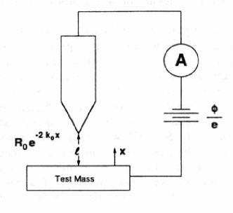
Figure 1: Scheme for the detection of displacement through a vacuum-tunneling transducer. The “at-rest” separation between the test mass and the tunneling probe is $l$ and the displacement of the test mass is $x$. The probe is voltage biased and the current is sensed by a current amplifier $A$.

When $|\partial T/\partial l|=0$ a second-order expansion must be employed; however, in all the situations which we explore in what follows, a first-order expansion of (5) is adequate.

In order to calculate the uncertainty in the momentum transferred to the barrier we first consider the continuity equation for the probability flux

$$\frac{\partial\rho}{\partial t}+\frac{\partial J}{\partial x}=0$$ (6)

where the probability density is

$$\rho=\psi^{*}\psi$$ (7)

and the probability current is

$$J=-i\frac{\hbar}{2m}\left[\psi^{*}\frac{\partial\psi}{\partial x}-\frac{\partial\psi^{*}}{\partial x}\psi\right].$$ (8)

Analogously for the momentum flux we have the following conservation equation:

$$\frac{\partial\rho}{\partial t}+\frac{\partial J_{p}}{\partial x}=-\frac{\partial V}{\partial x}\psi^{*}\psi,$$ (9)

where the momentum density is

$$\rho_{p}=-i\frac{\hbar}{2}\left[\psi^{*}\frac{\partial\psi}{\partial x}-\frac{\partial\psi^{*}}{\partial x}\psi\right].$$ (10)

and the momentum current is given by

$$J_{p}=\frac{\hbar^{2}}{4m}\left[2\frac{\partial\psi^{*}}{\partial x}\frac{\partial\psi}{\partial x}-\psi^{*}\frac{\partial^{2}\psi}{\partial x^{2}}-\frac{\partial^{2}\psi^{*}}{\partial x^{2}}\psi\right].$$ (11)

This progression can be carried out to higher moments of the momentum and for our calculation of the variance of the momentum we need to consider the flux of “momentum squared” for which the following continuity equation applies:

$$\frac{\partial\rho_{p^{2}}}{\partial t}+\frac{\partial J_{p^{2}}}{\partial x}=i\hbar\frac{\partial V}{\partial x}\left[\psi^{*}\frac{\partial\psi}{\partial x}-\frac{\partial\psi^{*}}{\partial x}\psi\right]$$ (12)

in which

$$\rho_{p^{2}}=-\frac{\hbar^{2}}{2}\left[\psi^{*}\frac{\partial^{2}\psi}{\partial x^{2}}-\frac{\partial^{2}\psi^{*}}{\partial x^{2}}\psi\right]$$ (13)

and

$$J_{p^{2}}=i\frac{\hbar^{3}}{4m}\left[\psi^{*}\frac{\partial^{3}\psi}{\partial x^{3}}-\frac{\partial\psi^{*}}{\partial x}\frac{\partial^{2}\psi}{\partial x^{2}}+\frac{\partial^{2}\psi^{*}}{\partial x^{2}}\frac{\partial\psi}{\partial x}-\frac{\partial^{3}\psi^{*}}{\partial x^{3}}\psi\right].$$ (14)

The above equations were derived by forming combinations of successive derivatives of the time-dependent one-dimensional Schrödinger equation for a particle in a potential $V(x)$ in much the same way as the familiar continuity equation (6) is derived. Note that (9) expresses Newton’s law in quantum mechanical terms, the right-hand side of (9) being the force density which acts on the particle. Also, a feature of (14) deserves comment. As we will see in the following examples $J_{p^{2}}$ is negative inside the barrier which is a consequence of the following. The barrier is a classically forbidden region so the kinetic energy flux $J_{p^{2}}/2m$ associated with a particle inside the barrier is negative which makes the “momentum squared” flux $J_{p^{2}}$ negative also.

Following Yurke and Kochanski’s approach let us imagine that the potential $V(x)$ represents a barrier located between $a<x<b$, and $V(x)$ is zero outside of this region. We decompose the force of the potential barrier on a tunneling particle into two parts, $\partial V/\partial x=\partial V_{1}/\partial x+\partial V_{2}/\partial x$, where $V_{1}$ is associated with the tunneling probe at the location $a$ and the potential $V_{2}$ is attributed to the test mass surface at $b$. To calculate the momentum uncertainty imparted to the test mass we must find the momentum and ’momentum-squared” fluxes passing through a surface at $b$. The momentum current transferred to the part of the barrier at $b$ is obtained by using the stationary version of (9) where $V(x)$ is replaced with $V_{2}(x)$, i.e.

$$J_{p}^{t}=J_{p}(b^{+})+\int_{a^{-}}^{b^{+}}\frac{\partial V_{2}}{\partial x}\psi^{*}\psi dx.$$ (15)

The “momentum squared” flux transferred to the barrier at $b$ is, using Eq. (12),

$$J_{p^{2}}^{t}=J_{p^{2}}(b^{+})-i\hbar\int_{a^{-}}^{b^{+}}\frac{\partial V_{2}}{\partial x}\left[\psi^{*}\frac{\partial\psi}{\partial x}-\frac{\partial\psi^{*}}{\partial x}\psi\right]dx$$ (16)

Dividing $J_{p}^{t}$ and $J_{p^{2}}^{t}$ by the incident flux $J_{\mathrm{i}n}$ we obtain the momentum and “momentum squared” transferred to the potential barrier at $b$ by a single tunneling particle. Finally, the momentum and “momentum squared” transferred to the test mass is related in the following fashion to the momentum and “momentum squared” transferred to the barrier from the electron. In our model, the test mass is schematized by a potential step at a fixed location in space. The test mass can be thought of as an infinitely rigid oscillator with a surface fixed at the location $b$; this is the effect of the feedback system which is actually used to prevent the test mass position from drifting under the effect of the continuous stream of electrons impinging on it. Therefore the test mass has a quantum-mechanical wave function which rapidly decays away from $b$. In a plane-wave representation, this corresponds to a superposition of plane waves with imaginary momenta. Thus a localized particle, in this case the test mass at $b$, with real momentum can be viewed as a free quasiparticle with imaginary momentum. Thus the mean momentum imparted to the test mass is $\langle p\rangle=iJ_{p}^{t}/J_{in}$ which is $i$ times the momentum transferred to the barrier from each electron tunneling event. As a consequence the mean “momentum squared” imparted to the test mass is $\langle p^{2}\rangle=-J_{p^{2}}^{t}/J_{in}$. The momentum fluctuation of the test mass due to $N$ electrons is then

$$(\Delta p)^{2}=N(\langle p^{2}\rangle-\langle p\rangle^{2})=N\left[-\frac{J_{p^{2}}^{t}}{J_{in}}+\left(\frac{J_{p}^{t}}{J_{in}}\right)^{2}\right].$$ (17)

In the following sections we will calculate the uncertainty product $\Delta l\Delta p$ for various stationary barriers when the electrons attempting to tunnel are initially in a momentum eigenstate.

To summarize the procedure outlined in this section the steps in the calculations will be the following. First we solve the time-independent Schrödinger equation to find the electron wave function in the presence of the barrier. From this we can calculate the transmission and reflection coefficients and therefore $\Delta l$ with the use of Eq. (5). Finally, we can find $\Delta p$ by using the solution of Schrödinger equation and the potential $V_{2}(x)$ in Eqs. (15)-(17).

III Uncertainty product for rectangular barriers

In this section we use the formalism developed in Sec. II to calculate the uncertainty product $\Delta l\Delta p$ for rectangular barriers, both symmetric [see Fig. 2(a)] and asymmetric [see Fig. 2(b)] cases.

In the symmetric barrier case the wave function which solves the time-independent Schrödinger equation can be expresses as

$$\psi_{k}(x) = \frac{1}{\sqrt{2\pi}}[e^{ikx}+r(k)e^{-ikx}],~{}~{}~{}~{}~{}x<a$$

$$\psi_{k}(x) = \frac{1}{\sqrt{2\pi}}[C^{+}(k)e^{k_{0}x}+C^{-}(k)e^{-k_{0}x}],~{}~{}~{}~{}~{}a<x<b$$ (18)

$$\psi_{k}(x) = \frac{1}{\sqrt{2\pi}}t(k)e^{ikx},~{}~{}~{}~{}~{}x>b,$$

where $\hbar k=\sqrt{2mE}$ and $\hbar k_{0}=\sqrt{2m(V_{0}-E)}$. The normalization of the wave function used throughout this paper corresponds to an incident flux $J_{in}=1/2\pi(\hbar k/m)$.

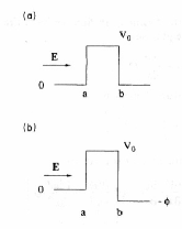
Figure 2: Potential energy for a rectangular barrier; symmetric (a) and asymmetric (b).

By imposing the matching conditions for $\psi$ and the first derivative of $\psi$ at $a$ and $b$ we obtain

$$t(k)=\frac{2ik_{0}ke^{-ik(b-a)}}{2ik_{0}k\cosh[k_{0}(b-a)]-(k_{0}^{2}-k^{2})\sinh[k_{0}(b-a)]}.$$ (19)

The uncertainty in the position $\Delta l$ can be calculated using Eq. (5):

$$\Delta l=\frac{1}{\sqrt{N}}\frac{1}{T}\frac{k}{(k^{2}+k_{0}^{2})\cosh(k_{0}l)},$$ (20)

where $l=b-a$ and the transmission coefficient is

$$T=|t(k)|^{2}=\frac{1}{1+\frac{(k_{0}^{2}+k^{2})\sinh^{2}[k_{0}(b-a)]}{4k_{0}^{2}k^{2}}}.$$ (21)

In order to calculate the momentum uncertainty we first define the potential due to the test mass as

$$V_{2}(x)=V_{0}\Theta(b-x).$$ (22)

Using Eqs. (15) and (16) we then have

$$J_{p}^{t}=\frac{1}{2\pi}\frac{\hbar^{2}}{2m}(k^{2}-k_{0}^{2})T,$$ (23)

$$J_{p^{2}}^{t}=-\frac{1}{2\pi}\frac{\hbar^{3}}{m}k_{0}^{2}kT.$$ (24)

According to (17), we get

$$(\Delta p)^{2}=N\frac{\hbar^{2}}{4k^{2}}T[4k^{2}k_{0}^{2}+(k^{2}-k_{0}^{2})^{2}T].$$ (25)

On multiplying $\Delta l$ and $\Delta p$ we obtain $\Delta l\Delta p=\hbar/2$, i.e., the minimum uncertainty product for the test mass. The uncertainty principle here may be regarded as arising from the interaction with the tunneling electrons during the process of measurement.

The same calculations can be repeated for an asymmetric rectangular barrier as in Fig. 2(b), schematizing an unbiased barrier between two materials having different work functions. The solution of the Schrödinger equation is

$$\psi_{k}(x) = \frac{1}{\sqrt{2\pi}}[e^{ikx}+r(k)e^{-ikx}],~{}~{}~{}~{}x<a$$

$$\psi_{k}(x) = \frac{1}{\sqrt{2\pi}}[C^{+}(k)e^{k_{0}x}+C^{-}(k)e^{-k_{0}x}],~{}~{}~{}~{}a\leq x<b$$ (26)

$$\psi_{k}(x) = \frac{1}{\sqrt{2\pi}}t(k)e^{i\bar{k}x},~{}~{}~{}~{}x>b,$$

where $\hbar k=\sqrt{2mE}$, $\hbar k_{0}=\sqrt{2m(V_{0}-E)}$, and $\hbar\bar{k}=\sqrt{2m(E+\phi)}$. The transmission amplitude is found to be

$$t(k)=\frac{2ik_{0}ke^{-i(\bar{k}b-ka)}}{ik_{0}(k+\bar{k})\cosh[k_{0}(b-a)]+(k\bar{k}-k_{0}^{2})\sinh[k_{0}(b-a)]}.$$ (27)

and the transmission coefficient is now defined as

$$T=\frac{\bar{k}}{k}|t(k)|^{2}.$$ (28)

To find the momentum uncertainty we can calculate the momentum flux and the “momentum-squared” flux transmitted to the barrier via the potential $V_{2}(x)=(V_{0}+\phi)\Theta(b-x)-\phi$ by applying (11) and (14):

$$J_{p}^{t}=\frac{1}{2\pi}\frac{\hbar^{2}}{2m}(\bar{k}^{2}-k_{0}^{2})\frac{k}{\bar{k}}T,$$ (29)

$$J_{p^{2}}^{t}=-\frac{1}{2\pi}\frac{\hbar^{3}}{m}k_{0}^{2}kT.$$ (30)

This allows us to evaluate $(\Delta p)^{2}$,

$$(\Delta p)^{2}=N\frac{\hbar^{2}}{4\bar{k}^{2}}T[4\bar{k}^{2}k_{0}^{2}+(\bar{k}^{2}-k_{0}^{2})^{2}T].$$ (31)

It is straightforward to show numerically that in this case the product of the uncertainties remains nearly the minimum allowed by quantum mechanics, i.e., $\hbar/2$, for any value of the potential energy $\varphi$.

IV Uncertainty product for a barrier with a constant electric field

We now repeat the above procedure for a barrier in which a constant electric field is present, such that the potential is expressed as (see Fig. 3)

$$V(x) = 0,~{}~{}~{}~{}x<a$$

$$V(x) = ,V_{0}-\phi\frac{x-a}{b-a},~{}~{}~{}~{}a\leq x<b$$ (32)

$$V(x) = -\phi,~{}~{}~{}~{}x>b.$$

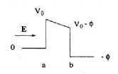
Figure 3: Potential energy for a barrier with a constant electric field.

The solution of Schrödinger’s time-independent equation is expressed as

$$\psi_{k}(x) = \frac{1}{\sqrt{2\pi}}[e^{ikx}+r(k)e^{-ikx}],~{}~{}~{}~{}x<a$$

$$\psi_{k}(x) = \frac{1}{\sqrt{2\pi}}[C^{+}(k)Ai[\alpha^{1/3}(\beta-x)]+C^{-}(k)Bi[\alpha^{1/3}(\beta-x)],~{}~{}~{}~{}a\leq x<b$$ (33)

$$\psi_{k}(x) = \frac{1}{\sqrt{2\pi}}t(k)e^{i\bar{k}x},~{}~{}~{}~{}x>b,$$

where $Ai(z)$ and $Bi(z)$ are the Airy functions with argument $z=\alpha^{1/3}(\beta-x)$ and $\alpha=(2m/\hbar^{2})\phi/(b-a)$, $\beta=a+[(V_{0}-E)/\phi](b-a)$. The quantities $k$ and $\bar{k}$ are defined as in the previous case of the asymmetric rectangular barrier.

After imposing the matching conditions we obtain

$$r(k) = -\frac{i}{2k}e^{ika}\{ik[C^{+}(k)Ai(\bar{a})+C^{-}(k)Bi(\bar{a})]+\alpha^{1/3}[C^{+}(k)Ai^{\prime}(\bar{a})+C^{-}(k)Bi^{\prime}(\bar{a})]\},$$ (34)

$$C^{+}(k) = \pi t(k)e^{\bar{k}b}[Bi^{\prime}(\bar{b})+i\bar{k}\alpha^{-1/3}Ai(\bar{b})],$$ (35)

$$C^{-}(k) = -\pi t(k)e^{i\bar{k}b}[Ai^{\prime}(\bar{b})+i\bar{k}\alpha^{-1/3}Ai(\bar{b})],$$ (36)

and

$$t(k)=-\frac{2ik}{\pi}e^{i(ka-\bar{k}b)}\alpha^{1/3}\{[\alpha^{1/3}Ai^{\prime}(\bar{a})-ikAi(\bar{a})][\alpha^{1/3}Bi^{\prime}(\bar{b})+i\bar{k}Bi(\bar{b})]-[\alpha^{1/3}Bi^{\prime}(\bar{a})-ikBi(\bar{a})][\alpha^{1/3}Ai^{\prime}(\bar{b})+i\bar{k}Ai(\bar{b})]\}^{-1},$$ (37)

where

$$\bar{b}=\alpha^{1/3}(\beta-b)$$ (38)

and

$$\bar{a}=\alpha^{1/3}(\beta-a)$$ (39)

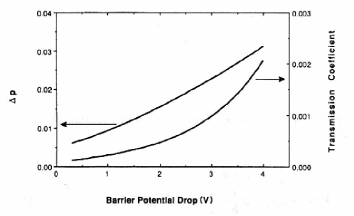
Figure 4: Momentum uncertainty in units where $\hbar=1$ (left scale) and transmission coefficient (right scale) for the rectangular barrier vs. the applied voltage.

The prime denotes the derivative with respect to the argument of the Airy function. The transmission and reflection coefficients are defined as

$$T=\frac{\bar{k}}{k}|t(k)|^{2},~{}~{}~{}~{}R=|r(k)|^{2}.$$ (40)

We introduce, as in the previous considerations, a potential $V_{2}(x)$ defined as

$$V_{2}(x)=\left[V_{0}-\frac{\phi}{2}\right]\Theta(a-x)+\Theta(x-a)\Theta(b-x)\left[V_{0}-\frac{\phi}{2}-\frac{\phi}{2}\frac{x-a}{b-a}\right]-\phi\Theta(x-b).$$ (41)

The momentum flux transmitted to the test mass can be calculated by

$$J_{p}^{t} = J_{p}(b^{+})+\int_{a^{+}}^{b^{-}}\frac{\partial V_{2}}{\partial x}|\psi(x)|^{2}dx+\int_{b^{-}}^{b^{+}}\frac{\partial V_{2}}{\partial x}|\psi(x)|^{2}dx=$$ (42)

$$J_{p}(b^{+})+\frac{1}{2}[J_{p}(a^{+})-J_{p}(b^{-})]+[J_{p}(b^{-})-J_{p}(B^{+})]=\frac{1}{2}[J_{p}(a^{+})+J_{p}(b^{-})].$$

Analogously, for $J_{p^{2}}^{t}$ we obtain

$$J_{p^{2}}^{t}=\frac{1}{2}[J_{p^{2}}(a^{+})+J_{p^{2}}(b^{-})].$$ (43)

Equations (15) and (16) can be used to express the fluxes inside the barrier in terms of the fluxes calculated outside the barrier. The detailed calculation of $\Delta p$ is shown in the Appendix, as well as the explicit form of the derivative of the transmission coefficient which allows us to obtain $\Delta l$.

In Fig. 4 the momentum uncertainty and the transmission coefficient are shown as functions of the applied voltage. We observe that as the potential drop across the barrier is increased the momentum uncertainty increases. This can be understood in the following way: when the electric field is increased the barrier is more transparent to the electrons and can be effectively represented by a lower rectangular barrier. Thus the electron current increases and $\Delta l$ is reduced. The uncertainty relation therefore requires a larger values of the momentum uncertainty.

In Fig. 5 the uncertainty product versus the applied voltage is shown for the case of $V_{0}=$5 eV and $E=$1 eV. The minimum uncertainty product is obtained in the absence of an applied voltage which can also be verified by examining the asymptotic behavior of the Airy functions in the limit of $\phi\rightarrow 0$. The increase of the uncertainty product $\Delta l\Delta p$ as the applied voltage is raised is due, at least in part, to a correlation between $\Delta l$ and $\Delta p$ induced by the electric field in the gap. The mechanism for the growth of the correlation is the following: an initial momentum dispersion of the electrons will be transformed into a spatial dispersion as the electrons traverse the barrier under the influence of the electric field. The magnitude of the correlation has been explicitly calculated in Ref. 8. A detailed discussion of the correlation between the uncertainties in momentum and position may be important for understanding techniques to surpass the standard quantum limit by using time-dependent tunnel probe bias voltages. This is a topic for further investigation.

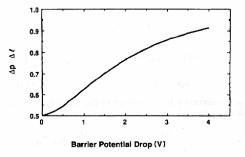
Figure 5: Uncertainty product $\Delta l\Delta p$ in units $\hbar=1$ for the test mass vs. the applied voltage in a rectangular barrier with a constant electric field. At a bias of 0 V, $\Delta l\Delta p=\hbar/2$, the value for a rectangular barrier.

V Practical configurations for reaching the quantum noise in tunneling transducers

In this section we discuss some experimental aspects of quantum measurements with a tunneling transducer. To compare the quantum noise with the classical sources of noise we have to introduce a “quantum” force noise spectral density which allows us to use the usual techniques of stochastic processes PRB9 . We do not claim to rigorously define such an effective noise spectral density, although it may be possible to define such a tool in the framework of Nelson’s stochastic mechanics PRB10 . Following Ref. 8 we write the spectral density of the force fluctuations in terms of the variance of the momentum current per unit bandwidth

$$S_{f_{Q}}=2\frac{(\Delta p)^{2}}{\tau},$$ (44)

where the effective force spectral density for the quantum noise has been expressed in terms of the uncertainty in the momentum deposited in the test mass by the tunneling current $I_{0}$ in a time interval $\tau$. In practical cases the bias voltage applied to the tunnel junction will be much less than the work function of the tip material so the rectangular barrier is a close approximation to reality. In this case the spectral density of the “quantum” force noise is

$$S_{f_{Q}}=\frac{I_{0}}{e}\hbar^{2}k^{2}\frac{1}{2}\left[\left(1+\left(\frac{k_{0}}{k}\right)^{2}\right)^{2}-\left(1-\left(\frac{k_{0}}{k}\right)^{2}\right)^{2}(1-T)\right].$$ (45)

The biggest practical obstacle to observing the quantum effects we discuss in this paper is the thermal noise which is manifested as the Brownian motion of the test mass. One can describe the Brownian motion of the test mass by including a Langevin force having a single-sided spectral density

$$S_{f_{L}}=4m(2\pi f_{0})\frac{k_{B}\theta}{Q}.$$ (46)

We assumed in Eq. (46) that the test mass is a mechanical resonator, at a temperature $\theta$, having mass $m$, frequency $f_{0}$, and quality factor $Q$ such that the decay time of the free oscillation is $Q/\pi f_{0}$. To be able to observe the influence of the tunneling transducer on the test mass the Langevin force must be smaller than the force fluctuations from the tunneling transducer, i.e., $S_{f_{Q}}>S_{f_{L}}$. This can be expressed in the following practical form:

$$\frac{10^{-6}{\mathrm{A}}}{I_{0}}\frac{m}{10^{-10}{\mathrm{k}g}}\frac{\theta}{10{\mathrm{m}K}}\frac{f_{0}}{10^{5}{\mathrm{H}z}}\frac{10^{7}}{Q}<1.$$ (47)

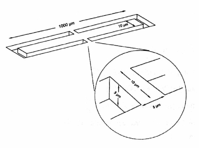
Figure 6: Design for a silicon micromachined torsional resonator with a resonant frequency of 60 KHz and an effective mass of $10^{-10}$ kg.

We have assumed that $k_{0}=10^{10}{\mathrm{m}}^{-1}$. The mass, frequency, and $Q$ used in (47) are appropriate to micromachined silicon resonators at low temperatures. The mass of $10^{-10}$ kg which is assumed above corresponds to a silicon structure like the one shown in Fig. 6. A mechanical quality factor of $6\times 10^{5}$ was obtained at room temperature in a micromachined silicon torsional resonator of mass $7\times 10^{-6}$ kg PRB11 , and a more massive resonator, $m\simeq 1$ g, which had a similar $Q$ at room temperature achieved a $Q$ approaching $10^{8}$ at 10 mK PRB12 . A systematic study of acoustic losses of silicon resonators at cryogenic temperatures indicates that the intrinsic $Q^{\prime}s$ of silicon are over one billion PRB13 . Therefore we assume that a $Q$ of $10^{7}$ may be achievable with a $10^{-10}$ kg mechanical resonator at 10 mK. Atomic force-sensing microcantilevers in this mass range have been fabricated and used at room temperature PRB14 .

There are two practical problems which are somewhat eased by working with a mechanical resonator at a frequency of 100 kHz. The first is the $1/f$ noise in the tunneling current. At a frequency of 100 kHz it is likely that the $1/f$ noise component in the tunneling current should be below the level of the shot noise. Furthermore there should be no problems with seismic vibrations and vibration isolation at the frequency of 100 kHz. Two other requirements to reach the quantum noise limit with the tunneling transducer are that the noise of the preamplifier used to sense the tunnel current be small in comparison to the shot noise and that the dynamic capacitance of the tunnel probe also be small. The first requirement, that the amplifier noise be insignificant compared to the tunneling current shot noise, is fairly easy to meet. For a tunneling current of $10^{-6}$ A the shot noise spectral density is $5.7\times 10^{-13}$ A/$\sqrt{\mathrm{H}z}$. This is a fairly high noise level compared to the noise of commonly available transistors and operational amplifiers PRB15 . The other requirement is that the dynamical capacitance, i.e., the probe capacitance which changes as the inverse of the tip to test mass gap, be “small”. Small in this context means low enough to ensure that the back-action force associated with fluctuations in the energy stored in the capacitor is less than the quantum force fluctuations of the tunneling current. The specific requirement on the dynamic capacitance have been calculated and values of $10^{-17}$ F or smaller are needed to reach the quantum limit PRB7 . There is also some experimental evidence that the dynamic capacitance of tunnel probes can be in this range PRB16 . Note that the stray probe capacitance, which may be orders of magnitude larger, is not important in this respect because it is only weakly gap dependent.

In the realm of conventional, nontunneling transducers, to overcome the two problems just discussed the so-called back-action evasion (BAE) techniques have been developed PRB2 . One example of a BAE strategy which has been used on a capacitive transducer coupled to a mechanical harmonic oscillator is to perform phase-sensitive detection. The coupling, i.e., the electric field in the capacitor formed between the transducer and the test mass, is modulated, which has the consequence that the back-action force acts on one of the phases of the mechanical oscillator while the information which is extracted from the mechanical oscillator reflects the state of the orthogonal phase. It is not clear if one can directly apply the phase-sensitive continuous-monitoring BAE techniques to the tunneling transducer and circumvent the quantum limit, however, one may be able to use a so-called quantum nondemolition stroboscopic measurement PRB2 . In this way, provided that an initial high-sensitivity measurement of the position has been made, repeated measurements made at time intervals of half the period of the mechanical oscillator motion can be performed with the same accuracy as the initial precise measurement. A stroboscopic measurement could be realized by sending in short pulses of tunneling current at time intervals equal to one-half of the period of the mechanical oscillator. One needs very short pulses to make an accurate stroboscopic measurement PRB17 . The duration of each pulse, and therefore the accuracy of the stroboscopic measurement, will be limited by the RC time constant of the tunneling probe so one will have to avoid large stray capacitance of the tunneling probe.

VI Conclusions

Quantum-mechanical uncertainties for measurements made on a test mass by a tunneling transducer have been calculated using a first-quantization approach.

The possibility of reaching the quantum limit in practical electromechanical devices incorporating a tunneling probe has been discussed, as well as a possible way to surpass the standard quantum limit by means of quantum nondemolition stroboscopic techniques.

in closing the ability to probe a single macroscopic object in the quantum domain opens a fundamental question concerning the validity of the quantum ergodicity assumption. This assumption is that ensemble averaged quantities are equivalent to time averages of the same quantity in a single quantum system. The point in our analysis where the quantum ergodicity assumption enters is Eq. (44), in which we assert the equivalence of the quantum uncertainties we calculated and the noise spectral densities of the corresponding quantities. All the experiments which probe microscopic quantum phenomena in which a measurement is made on each member of an ensemble of identically prepared systems have outcomes, without exception, which agree with the predictions of quantum mechanics. The sort of experiments which should be possible with the tunneling transducer are qualitatively different. One will be able to make repeated measurements on a single quantum system which is weakly coupled to its environment. In this case the outcome of the later measurements will depend upon the interaction of the measuring apparatus with the system during earlier measurements. If the ergodic assumption is true, then the outcome of the experiments discussed in this paper should coincide with the quantum predictions obtained by the usual ensemble-averaging technique.

APPENDIX

We use (15) and (16) for expressing the momentum density flux and the square momentum density flux inside the barrier in terms of the analogous quantities outside the barrier,

$$J_{p}(b^{-}) = J_{p}(b^{+})-\frac{|t(k)|^{2}}{2\pi}V_{0},$$ (48)

$$J_{p^{2}}(b^{-}) = J_{p^{2}}(b^{+})-\frac{|t(k)|^{2}}{2\pi}2V_{0}\hbar\bar{k},$$ (49)

$$J_{p}(a^{+}) = J_{p}(a^{-})-\frac{V_{0}}{2\pi}[1+R+2Re(re^{-2ika})],$$ (50)

$$J_{p^{2}}(a^{+}) = J_{p^{2}}(a^{-})-\frac{V_{0}}{2\pi}2\hbar k(1-R),$$ (51)

where the currents outside the barrier are

$$J_{p}(b^{+}) = \frac{|t(k)|^{2}}{2\pi}\frac{\hbar^{2}\bar{k}^{2}}{m},$$ (52)

$$J_{p^{2}}(b^{-}) = \frac{|t(k)|^{2}}{2\pi}\frac{\hbar^{3}\bar{k}^{3}}{m},$$ (53)

$$J_{p}(a^{+}) = \frac{1+R}{2\pi}\frac{\hbar^{2}k^{2}}{m},$$ (54)

$$J_{p^{2}}(a^{+}) = \frac{1-R}{2\pi}\frac{\hbar^{3}k^{3}}{m},$$ (55)

which, using (17), allows us to find $(\Delta p)^{2}$.

Finally the first derivative of the transmission coefficient with respect to the gap of the tunneling probe can be calculated and we find $\Delta l$ using (5):

$$\frac{dT}{dl}=\frac{\bar{k}}{k}\frac{d}{dl}|t(k)|^{2}=\frac{\bar{k}}{k}\left[\frac{dt(k)}{dl}t^{*}(k)+t(k)\frac{dt(k)^{*}}{dl}\right],$$ (56)

where the derivative of $t(k)$ is evaluated as

$$\frac{dt(k)}{dl}= t(k)\left[\alpha^{-1/3}\frac{d\alpha^{1/3}}{dl}-i(k+\bar{k})\right]+t(k)^{2}\frac{\pi}{2ik}\alpha^{-1/3}e^{i(\bar{k}b-ka)}$$

$$\times\biggl{[}\left\{[\alpha^{1/3}\bar{a}Ai(\bar{a})-ikAi^{\prime}(\bar{a})][\alpha^{1/3}Bi^{\prime}(\bar{b})+i\bar{k}Bi(\bar{b})]\right.$$

$$\qquad\left.-[\alpha^{1/3}\bar{a}Bi(\bar{a})-ikBi^{\prime}(\bar{a})][\alpha^{1/3}Ai^{\prime}(\bar{b})+i\bar{k}Ai(\bar{b})]\right\}\frac{d\bar{a}}{dl}$$

$$\quad+\left\{[\alpha^{1/3}Ai^{\prime}(\bar{a})-ikAi(\bar{a})][\alpha^{1/3}\bar{b}Bi(\bar{b})+i\bar{k}Bi^{\prime}(\bar{b})]\right.$$

$$\qquad\left.-[\alpha^{1/3}Bi^{\prime}(\bar{a})-ikBi(\bar{a})][\alpha^{1/3}\bar{b}Ai(\bar{b})+i\bar{k}Ai^{\prime}(\bar{b})]\right\}\frac{d\bar{b}}{dl}$$

$$\quad+\left\{[\alpha^{1/3}Bi^{\prime}(\bar{b})+i\bar{k}Bi(\bar{b})]Ai^{\prime}(\bar{a})+[\alpha^{1/3}Ai^{\prime}(\bar{a})-ikAi(\bar{a})]Bi^{\prime}(\bar{b})\right.$$

$$\qquad\left.-[\alpha^{1/3}Ai^{\prime}(\bar{b})+i\bar{k}Ai(\bar{b})]Bi^{\prime}(\bar{a})-[\alpha^{1/3}Bi^{\prime}(\bar{a})-ikBi(\bar{a})]Ai^{\prime}(\bar{b})\right\}\frac{d\alpha^{1/3}}{dl}\biggr{]},$$ (57)

taking into account the following relationships:

$$\frac{dt^{*}(k)}{dl} = \left[\frac{dt(k)}{dl}\right]^{*},$$ (58)

$$\frac{d\bar{a}}{dl} = \frac{2}{3}\left[\frac{2m\phi}{\hbar^{2}}\right]^{1/3}\frac{V_{0}-E}{\phi}l^{-1/3},$$ (59)

$$\frac{d\bar{b}}{dl} = \frac{2}{3}\left[\frac{2m\phi}{\hbar^{2}}\right]^{1/3}\left[\frac{V_{0}-E}{\phi}-1\right]{\varphi}l^{-1/3},$$ (60)

$$\frac{d\alpha^{1/3}}{dl} = -\frac{1}{3}\frac{\alpha^{1/3}}{l}.$$ (61)

References

- (1) See, for example, K. S. Thorne, in Three Hundred Years of Gravitation, edited by S. Hawking and W. Israel (Cambridge University Press, Cambridge, 1987).
- (2) C. M. Caves, K. S. Thorne, R. P. Drever, V. D. Sandberg, and M. Zimmermann, Rev. Mod. Phys. 52, 341 (1980).
- (3) M. F. Bocko and W. W. Johnson, in New Techniques and Ideas in Quantum Measurement Theory, edited by D.M. Greenberger (New York Academy of Sciences, New York, N.Y.) 1986, Vol. 480.
- (4) R. Onofrio, Europhys. Lett. 11, 695 (1990).
- (5) M. F. Bocko, Rev. Sci. Instrum. 61, 3763 (1990).
- (6) Bocko M.F., Stephenson K.A. and Koch R.H., Phys. Rev. Lett. 61 726 (1988).
- (7) K. A. Stephenson, M. F. Bocko, and R. H. Koch, Phys. Rev. A 40, 6615 (1989).
- (8) B. Yurke and G. P. Kochanski, Phys. Rev. B 41, 8184 (1990).
- (9) See, for example, A. Papoulis, Signal Analysis (McGraw-Hill, new York, 1977).
- (10) E. Nelson, Quantum Fluctuations (Princeton University Press, Princeton, 1985).
- (11) R. A Buser and N. F. De Rooij, Sensors and Actuators A 21-A23, 323 (1990).
- (12) G. Kaminsky, J. Vac. Sci. Technol. B 3, 1015 (1985).
- (13) C. C. Lam, Ph.D. thesis, University of Rochester, 1979.
- (14) S. Akamine, R. C. Barrett, and C.F. Quate, Appl. Phys. Lett. 57, 316 (1990).
- (15) Designing with Field Effect Transistors, edited by A.D. Evans (McGraw-Hill, New York, 1981).
- (16) P. J. van Bentum, H. van Kempen, L. E. C. van de Leemput, and P. A. A. Teunissen, Phys. Rev. Lett. 60, 369 (1988).
- (17) R. Onofrio, Phys. Lett. A 148, 1 (1990).