Simple one–dimensional quantum–mechanical model for a particle attached to a surface

Abstract

We present a simple one–dimensional quantum–mechanical model for a particle attached to a surface. We solve the Schrödinger equation in terms of Weber functions and discuss the behavior of the eigenvalues and eigenfunctions. We derive the virial theorem and other exact relationships as well as the asymptotic behaviour of the eigenvalues. We calculate the zero–point energy for model parameters corresponding to H adsorbed on Pd(100) and also outline the application of the Rayleigh–Ritz variational method.

I Introduction

In an introductory course on quantum theory one commonly discusses some of the simplest models, such as, for example: free particle, particle in a box, harmonic oscillator, tunnelling through a square barrier, etc. with the purpose of making the students more familiar with the principles or postulates of quantum theory. Some time ago GibbsG75 introduced the quantum bouncer as a model for the pedagogical discussion of some of the relevant features of quantum theory. He derived the solutions to the Schrödinger equation in terms of Airy functions and obtained the energy spectrum for two different model settings.

A closely related model, the harmonic oscillator with a hard wall on one side, had been discussed earlier by DeanD66 and later by Mei and LeeML83 . This model is as simple as the quantum bouncer and both can therefore be discussed in the same course. An interesting feature of this model is that it may in principle be useful to simulate a particle attached to a wall like, for example, an atom adsorbed on a solid surfaceRPG69 ; GKKSSO10 . Although it is an oversimplified one–dimensional model of the actual physical phenomenon we deem it worthwhile to discuss some of its properties in this paper.

In Sec. II we introduce the model, write the Schrödinger equation in dimensionless form, and discuss some of the properties of its solutions. In Sec. III we obtain the eigenfunctions and eigenvalues explicitly in terms of the well known Weber functionsMF53 and show the behavior of the eigenvalues and excitation energies with respect to the distance between the particle and the wall. We also calculate the zero–point energy for values of the model parameters corresponding to de adsorption of H on Pd(100)GKKSSO10 and outline the application of the Rayleigh–Ritz variational method to the Schrödinger equation. Finally, is Sec. IV we give further reasons why this model may be useful in a course on quantum theory.

II Simple model

We consider a simple one–dimensional model for a particle of mass $m$ attached to a surface located at $x=0$ that separates free space ($x>0$) from the bulk of the material ($x<0$). Therefore, we assume that the potential exhibits an attractive tail for $x>0$ that keeps the particle in the neighborhood of the surface and a repulsive one for $x<0$ that prevents the particle from penetrating too deep into the material. Since we want to keep the model as simple as possible we choose

$$V(x)=\left\{\begin{array}[]{c}\infty\text{ if }x<0\\ \frac{k}{2}(x-d)^{2}\text{ if }x\geq 0\end{array}\right.$$ (1)

where $k,d>0$. We note that the particle oscillates about $x=d$ but the motion is not harmonic because of the effect of the hard wall.

The Schrödinger equation reads

$$- \frac{\hbar^{2}}{2m}\psi^{\prime\prime}(x)+\frac{k}{2}(x-d)^{2}\psi(x)=E\psi(x)$$ (2)

$$\psi(0)=0,\,\lim_{x\rightarrow\infty}\psi(x)=0$$

where the boundary condition at $x=0$ comes from the fact that in this simple model the particle cannot penetrate into the material and, consequently, $\psi(x)=0$ for all $x<0$. Since it is more convenient to work with a dimensionless equation we define the length unit $L=\left(\frac{\hbar^{2}}{km}\right)^{1/4}$ and the dimensionless coordinate $q=(x-d)/L$. Thus, the dimensionless Schrödinger equation reads

$$- \frac{1}{2}\varphi^{\prime\prime}(q)+\frac{1}{2}q^{2}\varphi(q)=\epsilon\varphi(q)$$ (3)

$$\varphi(-q_{0})=0,\,\lim_{q\rightarrow\infty}\varphi(q)=0$$

where

$$\epsilon=\frac{mL^{2}E}{\hbar^{2}}=\frac{E}{\hbar\omega},\text{\thinspace}\omega=\sqrt{\frac{k}{m}}$$

$$q_{0}=\frac{d}{L}=d\left(\frac{km}{\hbar^{2}}\right)^{1/4}$$

$$\varphi(q)=\psi(Lq+d)$$ (4)

It is worth noting that $q_{0}$ increases with $d$, $m$, and $k$. It is precisely Eq. (3) that was discussed by DeanD66 and Mei and LeeML83 .

When $q_{0}\rightarrow\infty$ we have the well–known harmonic oscillator with eigenvalues

$$\lim_{q_{0}\rightarrow\infty}\epsilon_{n}=n+\frac{1}{2},\,n=0,1,\ldots$$ (5)

On the other hand, when $q_{0}=0$ we have the harmonic oscillator in the half line and

$$\lim_{q_{0}\rightarrow 0}\epsilon_{n}=2n+\frac{3}{2},\,n=0,1,\ldots$$ (6)

Note that these are merely the harmonic–oscillator eigenvalues with odd quantum number (the corresponding eigenfunctions have a node at origin). It follows from Eq. (32) in the Appendix that

$$\frac{d\epsilon}{dq_{0}}<0,\;\lim_{q_{0}\rightarrow\infty}\frac{d\epsilon}{dq_{0}}=0$$ (7)

from which we conclude that the energy eigenvalues decrease monotonously between the following limits:

$$2n+\frac{3}{2}\geq\epsilon_{n}(q_{0})>n+\frac{1}{2},\,n=0,1,\ldots$$ (8)

when $0\leq q_{0}<\infty$. It should be kept in mind that the number of zeros of $\varphi_{n}(q)$ remains unchanged as $q_{0}$ goes from $0$ to $\infty$.

Equation (32) is useful for obtaining the asymptotic behavior of the energy as $q_{0}\rightarrow\infty$. To this end we simply integrate it from $-\infty$ to $-q_{0}$:

$$\epsilon(-q_{0})=\epsilon(-\infty)+\frac{1}{2}\int_{-\infty}^{-q_{0}}\frac{\varphi^{\prime}(b)^{2}}{\int_{b}^{\infty}\varphi(q)^{2}\,dq}\,db$$ (9)

For the ground state we expect that $\varphi(q)\rightarrow Ne^{-q^{2}/2}$ as $q_{0}\rightarrow\infty$. The normalization factor is approximately given by

$$N^{-2}(q_{0})=\int_{-q_{0}}^{\infty}e^{-q^{2}}\,dq=\frac{\sqrt{\pi}}{2}[1+\mbox{erf}(q_{0})]$$ (10)

where $\mbox{erf}(z)$ is the error function. Since $\mbox{erf}(z)\leq\mbox{erf}(\infty)=1$ we write $\mbox{erf}(q_{0})=1-\xi$ and expand $N^{2}$ in a Taylor series about $\xi=0$:

$$N(q_{0})^{2}\approx\frac{2+\xi}{2\sqrt{\pi}}=\frac{3-\mbox{erf}(q_{0})}{2\sqrt{\pi}}$$ (11)

Finally, Eq. (9) yields

$$\epsilon_{0}(-q_{0})\approx\frac{1}{2}+\frac{q_{0}e^{-q_{0}^{2}}}{2\sqrt{\pi}}$$ (12)

In order to obtain this result we substituted $\mbox{erf}(q_{0})\approx 1$ after the integration and neglected a term proportional to $e^{-2q_{0}^{2}}$ because it is much smaller than the exponential one retained in Eq. (12). This result agrees with the one derived by Mei and LeeML83 by means of perturbation theory (note that their parameter $R$ is $\sqrt{2}q_{0}$).

Proceeding in the same way for the first excited state we obtain

$$\epsilon_{1}(-q_{0})\approx\frac{3}{2}+\frac{q_{0}(2q_{0}^{2}-1)e^{-q_{0}^{2}}}{2\sqrt{\pi}}$$ (13)

that is slightly different from the result of Mei and LeeML83 . However, they are equivalent for most purposes because the difference between them is smaller than their absolute errors.

Eq. (36) gives us the virial theoremFC87 for this model

$$\left\langle\hat{D}^{2}\right\rangle+\left\langle q^{2}\right\rangle=q_{0}\frac{\partial\epsilon}{\partial q_{0}}$$ (14)

where $\hat{D}=d/dq$. The right–hand side of this equation is the virial of the force exerted by the surface. Eq. (39) provides us with another interesting relation

$$\left\langle q\right\rangle=-\frac{\partial\epsilon}{\partial q_{0}}$$ (15)

that clearly reveals the asymmetry of the interaction between the particle and the surface. In both cases we recover the well–known results for the harmonic oscillator $\left\langle\hat{D}^{2}\right\rangle+\left\langle q^{2}\right\rangle=0$ and $\left\langle q\right\rangle=0$ when $q_{0}\rightarrow\infty$.

III Results

If we define the new independent variable $z=\sqrt{2}q$ and write the energy as $\epsilon=m+1/2$ then we realize that $D_{m}(z)=\varphi(z/\sqrt{2})$ is a solution to the Weber equationMF53

$$D_{m}^{\prime\prime}(z)+\left(m+1/2-z^{2}/4\right)D_{m}(z)=0$$ (16)

The general solution isMF53

$$D_{m}(z)=2^{m/2}\sqrt{\pi}e^{-z^{2}/4}\left[\frac{1}{\Gamma(\frac{1-m}{2})}F\left(-\frac{m}{2}\left|\frac{1}{2}\right|\frac{z^{2}}{2}\right)-\frac{\sqrt{2}z}{\Gamma(-\frac{m}{2})}F\left(\frac{1-m}{2}\left|\frac{3}{2}\right|\frac{z^{2}}{2}\right)\right]$$ (17)

where the confluent hypergeometric function $F\left(a\left|c\right|z\right)$ is a solution to

$$zF^{\prime\prime}(z)+(c-z)F(z)-aF(z)=0$$ (18)

and can be expanded in a Taylor series about $z=0$ as

$$F\left(a\left|c\right|z\right)=1+\frac{a}{c}z+\frac{a(a+1)}{2!c(c+1)}z^{2}+\ldots$$ (19)

The boundary condition $\varphi(-q_{0})=0$ enables us to calculate the eigenvalues from the roots of $D_{m}\left(-\sqrt{2}q_{0}\right)=0$. For each value of $q_{0}$ we solve

$$\frac{1}{\Gamma(\frac{1-m}{2})}F\left(-\frac{m}{2}\left|\frac{1}{2}\right|q_{0}^{2}\right)+\frac{2q_{0}}{\Gamma(-\frac{m}{2})}F\left(\frac{1-m}{2}\left|\frac{3}{2}\right|q_{0}^{2}\right)=0$$ (20)

for $m$ and then calculate the dimensionless energy $\epsilon=m+1/2$. This approach has already been discussed by DeanD66 and Mei and LeeML83 .

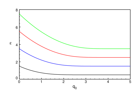
Figure 1: (Color online) First four energy levels

Fig. 1 shows $\epsilon_{n}(q_{0})$ for $n=0,1,2,3$ and a wide range of values of $q_{0}$. We note that the dimensionless energy decreases monotonously as predicted by Eq. (7) between the limits indicated in Eq. (8).

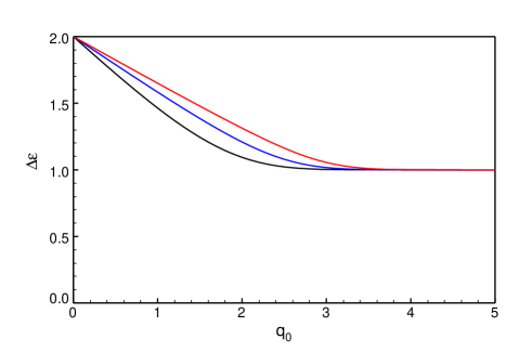
Figure 2: (Color online) The first three excitation energies $\epsilon_{n+1}-\epsilon_{n}$ ($n=0,1,2$ from bottom to top)

The gap between two consecutive energy levels of the harmonic oscillator is $\Delta\epsilon_{n}=\epsilon_{n+1}-\epsilon_{n}=1$ ($\Delta E_{n}=\hbar\omega$). Fig. 2 shows $\Delta\epsilon_{n}(q_{0})$ for $n=0,1,2$ where we note that the energy gap increases with $n$ revealing that the presence of the wall results in an anharmonic oscillation. It becomes more harmonic as $q_{0}$ increases (by increasing either $d$, $m$ or $k$).

In order to have a clearer physical idea of the kind of predictions of this simple model we may choose the parameters for the adsorption of hydrogen on Pd(100). Gladys et alGKKSSO10 estimated $d\approx 0.4\,$Å and $k\approx 15\,N\,m^{-1}$ for hydrogen that lead to $q_{0}\approx 1.55$. The zero–point energy for such model parameters is approximately $0.57\,\hbar\,\omega$ instead of the value $\hbar\,\omega/2$ chosen by those authors. Although they fitted the potential energy of the vertical displacement of the H atom from the Pd surface to a cubic polynomial they simply chose the zero–point energy of the harmonic oscillator. Present model predicts that the zero–point energy is slightly greater than the harmonic–oscillator one because of the repulsive effect of the surface. We agree that a hard wall may not be the most adequate representation of the short–range interaction between the H atom and the Pd surface, but we think that the model is a reasonably simple first approach to the physical phenomenon.

For deuterium we have $d\approx 0.45\,$Å which, together with the same force constant and about twice the mass, yields $q_{0}\approx 2$ and $\epsilon_{0}\approx 0.52\,\hbar\,\omega$ that is closer to the harmonic–oscillator zero–point energyGKKSSO10 . We note the effect of the distance to the surface and the mass of the particle on the vibrational energies.

This model is also useful for discussing the Rayleigh–Ritz variational methodMF53 . If, for example, we choose the trial function

$$u(q)=\sum_{j=0}^{N-1}c_{j}f_{j}(q)$$ (21)

as a linear combination of the non orthogonal basis set

$$f_{j}(q)=(q+q_{0})q^{j}e^{-q^{2}/2},\;j=0,1,\ldots$$ (22)

and minimize the approximate energy

$$w = \frac{\int_{-q_{0}}^{\infty}u(q)\hat{H}u(q)\,dq}{\int_{-q_{0}}^{\infty}u(q)^{2}\,dq}$$

$$\hat{H} = -\frac{1}{2}\frac{d^{2}}{dq^{2}}+\frac{1}{2}q^{2}$$ (23)

then we arrive at the secular equations

$$\sum_{j=0}^{N-1}\left(H_{ij}-wS_{ij}\right)c_{j}=0,\;i=0,1,\ldots,N-1$$

$$H_{ij}=\int_{-q_{0}}^{\infty}f_{i}(q)\hat{H}f_{j}(q)\,dq,\;S_{ij}=\int_{-q_{0}}^{\infty}f_{i}(q)f_{j}(q)\,dq$$ (24)

There are nontrivial solutions for the coefficients $c_{j}$ only if the secular determinant vanishes

$$\left|H_{ij}-wS_{ij}\right|_{i,j=0}^{N-1}=0$$ (25)

Its roots $w_{n}^{[N]}$, $n=0,1,\ldots,N-1$ are upper bounds to the actual eigenvalues and satisfy

$$w_{n}^{[N]}>w_{n}^{[N+1]}>\epsilon_{n}$$ (26)

The particle attached to a wall is therefore a suitable example for illustrating how the roots of the secular determinant approach the eigenvalues (calculated accurately from the Weber functions) from above as $N$ increases. We do not show results here and simply mention that the calculation is greatly facilitated by the fact that one calculates the integrals $H_{ij}$ and $S_{ij}$ analytically.

IV Further comments

The model discussed here is suitable for a course on quantum theory because it does not require much more mathematical background than it is necessary for the discussion of the well known harmonic oscillator or the quantum bouncerG75 . It is useful for introducing a numerical calculation of the eigenvalues that the student does not find in the treatment of the harmonic oscillator. One can approach the problem by means of either the Weber functions or the Rayleigh–Ritz variational method. The student will also learn that it is necessary to modify the form of the well known virial theorem and other mathematical expressions in order to take into account the effect of the wall. We believe that present derivation of the analytical results in Sec. II and in the Appendix is simpler than those available in the scientific literatureD66 ; ML83 .

In addition to it, the model enables us to simulate the adsorption of an atom on a surface and discuss anharmonic vibrations in quantum theory. In the study of molecular vibrations one introduces nonlinear oscillations by means of cubic, quartic, and other terms of greater degree in the potential–energy function. In this case it arises from the boundary condition forced by the hard wall.

*

Appendix A Some useful mathematical relations

In this appendix we develop some useful analytical results for the eigenfunctions and eigenvalues of the constrained oscillator. Although similar expressions have already been shown elsewhereFC87 we derive them here in a form that is more suitable for our needs.

Consider the dimensionless Schrödinger equation

$$- \frac{1}{2}\varphi^{\prime\prime}(x)+V(x)\varphi(x)=\epsilon\varphi(x)$$ (27)

$$\varphi(b)=0,\,\lim_{x\rightarrow\infty}\varphi(x)=0$$

Both the eigenvalue $\epsilon$ and the eigenfunction $\varphi(x)$ depend on the chosen value of $b$. If we differentiate this equation with respect to $b$ and call $\chi(x)=\partial\varphi(x)/\partial b$ we have

$$-\frac{1}{2}\chi^{\prime\prime}(x)+V(x)\chi(x)=\epsilon\chi(x)+\frac{d\epsilon}{db}\varphi(x)$$ (28)

If we multiply this equation by $\varphi(x)$ and integrate the result between $b$ and $\infty$ we easily obtain

$$\frac{d\epsilon}{db}\int_{b}^{\infty}\varphi(x)^{2}\,dx=-\frac{1}{2}\chi(b)\varphi^{\prime}(b)$$ (29)

because the integration by parts of the first term yields

$$\int_{b}^{\infty}\chi^{\prime\prime}(x)\varphi(x)\,dx=\chi(b)\varphi^{\prime}(b)+2\int_{b}^{\infty}\left[V(x)-\epsilon\right]\chi(x)\varphi(x)\,dx$$ (30)

If we now differentiate the boundary condition $\varphi(b)=0$ and take into account that $\varphi(x)$ depends on $b$ we obtain

$$\chi(b)+\varphi^{\prime}(b)=0$$ (31)

so that equation (29) becomes

$$\frac{d\epsilon}{db}\int_{b}^{\infty}\varphi(x)^{2}\,dx=\frac{1}{2}\varphi^{\prime}(b)^{2}$$ (32)

We define the operators

$$\hat{H}=-\frac{1}{2}\hat{D}^{2}+V(x)$$ (33)

and $\hat{v}=\hat{x}\hat{D}$, where $\hat{D}=d/dx$. The commutator between them reads

$$[\hat{H},\hat{v}]=\hat{H}\hat{v}-\hat{v}\hat{H}=-\hat{D}^{2}-xV^{\prime}$$ (34)

If $\varphi(x)$ is an eigenfunction of $\hat{H}$ with eigenvalue $\epsilon$ then straightforward integration by parts leads to

$$\int_{b}^{\infty}\varphi[\hat{H},\hat{v}]\varphi\,dx=-\frac{1}{2}b\varphi^{\prime}(b)^{2}$$ (35)

which, by virtue of Eq. (32), becomes the virial theorem

$$\left\langle\hat{D}^{2}\right\rangle+\left\langle xV^{\prime}\right\rangle=b\frac{\partial\epsilon}{\partial b}$$ (36)

where

$$\left\langle\hat{A}\right\rangle=\frac{\int_{b}^{\infty}\varphi\hat{A}\varphi\,dx}{\int_{b}^{\infty}\varphi^{2}\,dx}$$ (37)

Analogously, from the commutator $[\hat{H},\hat{D}]=-V^{\prime}$ we obtain

$$\int_{b}^{\infty}\varphi(x)^{2}V^{\prime}(x)\,dx=\frac{1}{2}\varphi^{\prime}(b)^{2}$$ (38)

or

$$\left\langle V^{\prime}\right\rangle=\frac{\partial\epsilon}{\partial b}$$ (39)

We can test these equations quite easily by means of the well–known solutions to the free harmonic oscillator

$$\psi_{n}=N_{n}H_{n}(x)e^{-x^{2}/2}$$ (40)

where $H_{n}(x)$ is a Hermite polynomial and $N_{n}$ the corresponding normalization factorMF53 . If we choose $b$ to be one of the zeroes $x_{nj}$, $j=1,2,\ldots,n$ of $H_{n}(x)$, $n=1,2,\ldots$ then we verify that $\psi_{n}(x)$ satisfies equations (35) and (38) for $V(x)=x^{2}/2$. If, for example, $b=0$ for $n=1$ and $b=\pm 1/\sqrt{2}$ for $n=2$ then $\epsilon=3/2$ is the energy of the ground state of the harmonic oscillator with the boundary condition at $b=0$ and $\epsilon=5/2$ is the energy of the ground state with $b=1/\sqrt{2}$ and of the first excited state with $b=-1/\sqrt{2}$.

References

- (1) R. L. Gibbs, “The quantum bouncer”, Amer. J. Phys. 43, 25-28 (1975).
- (2) P. Dean, “The constrained quantum mechanical harmonic oscillator”, Proc. Camb. Phil. Soc. 62, 277-286 (1966).
- (3) W. N. Mei and Y. Lee, “Harmonic oscillator with potential barriers-exact solutions and perturbative treatments”, J. Phys. A 16, 1623-1632 (1983).
- (4) F. Ricca, C. Pisani, and E. Garrone, “States of Helium atoms adsorbed on Krypton and Xenon crystals”, J. Chem. Phys. 51, 4079-4091 (1969).
- (5) M. J. Gladys, I. Kambali, M. A. Karolewski et al., “Comparison of hydrogen and deuterium adsorption on Pd(100)”, J. Chem. Phys. 132, 024714 (8 pp) (2010).
- (6) P. M. Morse and H. Feschbach, Methods of Theoretical Physics, (McGraw-Hill, New York, 1953).
- (7) F. M. Ferńandez and E. A. Castro, Hypervirial Theorems, Lecture Notes in Chemistry, (Springer-Verlag, Berlin, 1987).