Fractional bidromy in the vibrational spectrum of HOCl

Abstract

We introduce the notion of fractional bidromy which is the combination of fractional monodromy and bidromy, two recent generalizations of Hamiltonian monodromy. We consider the vibrational spectrum of the HOCl molecule which is used as an illustrative example to show the presence of nontrivial fractional bidromy. To our knowledge, this is the first example of a molecular system where such a generalized monodromy is exhibited.

The description and the understanding of molecular spectra have been a long-standing goal in the field of molecular physics, both from experimental and theoretical points of view (for recent reviews, see [1, 2] and references therein). Vibrational dynamics of sufficiently rigid polyatomic molecules can be well reproduced up to a large fraction of the dissociation threshold by an effective Hamiltonian which is obtained either by a fit of parameters to a set of measured or calculated energy levels [3] or by the application of canonical perturbation theory to an ab initio potential energy surface [4]. An important class of effective Hamiltonians are the classically integrable Hamiltonians, which allow to simplify the study of the dynamics of the system by the use of constants of the motion. Among them, we can distinguish the simplest one, the Dunham expansion, which in the absence of strong resonances describes accurately the vibrational dynamics at low energy near a minimum of the potential energy surface. This effective Hamiltonian can be written as a polynomial expansion in terms of the actions of the normal modes, which can be defined globally on the whole phase space. Resonant Hamiltonians, i.e., effective Hamiltonians with fundamental frequencies in resonance [1], describe the dynamics at higher energies where the coupling between, at least, two degrees of freedom cannot be neglected. Even if Hamiltonians of this kind are integrable, i.e., the number of constants of the motion is equal to the number of degrees of freedom, their classical dynamics may not be globally described by action-angle variables since the latter are in general only locally defined. The question that naturally arises is how to detect this feature both from the classical and quantum points of view. Indeed, the fact that the actions are only local has a quantum counterpart in the joint spectrum of the quantum Hamiltonian as it prevents the existence of global quantum numbers [5].

In this context, monodromy, which is the simplest topological obstruction to the existence of a global set of action-angle variables, has become a useful tool both in classical [6, 7, 8] and quantum or semi-classical mechanics [5, 8]. First discovered and developed by mathematicians, the phenomenon of monodromy has been exhibited in a large variety of physical systems extending from atomic and molecular ones [9] to purely classical systems [7, 10]. Such systems have a standard monodromy which is either characterized by an isolated focus-focus singularity in the associated bifurcation diagram for the local case or by a second leaf which is glued to the main leaf through a line of bitori for the nonlocal situation [2]. Both types of monodromies appear in Fermi resonant systems with a non zero angular momentum [11]. Recently, different kinds of generalized monodromy, such as fractional monodromy [12] and bidromy [13, 14], have been defined and their presence shown in model Hamiltonian systems (see below for a concrete definition of these generalizations). The next step in this study is the determination of physical systems having such monodromies. It is in this spirit that we revisit the analysis of the vibrational dynamics of the HOCl molecule with zero angular momentum. We show the presence in this molecular spectrum of nontrivial fractional bidromy which can be viewed as the combination of fractional monodromy and bidromy. We first describe the corresponding bifurcation diagram, which presents a line of curled tori and a line of bitori. Fractional bidromy is defined through a bipath, i.e., a set of two loops, which are allowed to cross both lines of curled tori and bitori. This is a specificity of generalized monodromies with respect to standard ones for which the associated loop lies in the set of regular values of the bifurcation diagram. We determine the quantum monodromy matrix for a bipath such that only one of its two components crosses the line of curled tori. Conclusion and prospective views are given in the last section.
Vibrational dynamics of HOCl. Several studies have investigated the vibrational dynamics of HOCl both from the experimental and theoretical points of view (details can be found in [15] and references therein). In particular, although very accurate ab initio calculations have been undertaken, it has been shown that the use of an effective Hamiltonian allows an original and precise understanding of the qualitative features of the dynamics [15]. This effective Hamiltonian includes energy levels of the ground electronic state with an energy up to 98 $\%$ of the dissociation energy. The classical Hamiltonian $H$ is expressed in terms of the normal modes coordinates $(q_{1},p_{1},q_{2},p_{2},q_{3},p_{3})$. $q_{1}$, $q_{2}$ and $q_{3}$ are close respectively to the Jacobi coordinates $(r,\gamma,R)$, where $r$ is the OH bond length, $R$ the distance from Cl to the center of mass G of OH ($R$ is very close to the OCl bond length) and $\gamma$ the OGCl angle ($\gamma=0$ at linear HOCl geometry). $H$ can be written as the sum of two terms $H=H_{D}+H_{F}$ where the Dunham expansion $H_{D}$ and the resonant part $H_{F}$ are respectively equal to

$$H_{D} = \sum_{i=1}^{3}\frac{\omega_{i}}{2}(p_{i}^{2}+q_{i}^{2})+\sum_{i\geq j}\frac{x_{ij}}{4}(p_{i}^{2}+q_{i}^{2})(p_{j}^{2}+q_{j}^{2})+$$

$$\sum_{i\geq j\geq k}\frac{y_{ijk}}{8}(p_{i}^{2}+q_{i}^{2})(p_{j}^{2}+q_{j}^{2})(p_{k}^{2}+q_{k}^{2})+\cdots,$$

$$H_{F} = \frac{1}{\sqrt{2}}[(q_{3}^{2}-p_{3}^{2})q_{2}+2q_{3}p_{3}p_{2}](k+\sum_{i}\frac{k_{i}}{2}(p_{i}^{2}+q_{i}^{2})+$$

$$\sum_{i\geq j}\frac{k_{ij}}{4}(p_{i}^{2}+q_{i}^{2})(p_{j}^{2}+q_{j}^{2})+\cdots).$$

The parameters $\omega_{i}$, $x_{ij}$, $y_{ijk}$, $z_{ijkl}$, $k$, $k_{i}$ and $k_{ij}$ for HOCl can be found in [15]. Since the functions $I_{1}=(p_{1}^{2}+q_{1}^{2})/2$, $I=p_{2}^{2}+q_{2}^{2}+(p_{3}^{2}+q_{3}^{2})/2$ and $H$ are constants of the motion, the system is integrable. An additional 3:1 resonance between the modes 1 and 2 can also be considered but we neglect it in this paper since it renders the effective Hamiltonian non integrable.
Bifurcation diagram. Before describing the classical bifurcation diagram, we have to say some words about the quantum problem. The quantization rules for nondegenerate vibrations are [15]

$$\left\{\begin{array}[]{ll}I_{1}=\hbar(v_{1}+\frac{1}{2})\\ I=\hbar(P+\frac{3}{2})\end{array}\right.,$$ (3)

where $v_{1}$ and $P=2v_{2}+v_{3}$ are respectively the number of quanta in the OH stretching degree of freedom and the polyad number. $v_{1}$ and $P$ are the quantum numbers associated to the classical constants of the motion $I_{1}$ and $I$. The constant $\hbar$ is an effective Planck constant which can, at least theoretically, be modified at will to increase the density of energy levels. This is necessary since the notion of quantum Hamiltonian monodromy is only defined rigorously in the semi-classical limit where $\hbar\to 0$ [5]. The value $\hbar=1$ corresponds to the physical problem [15].

From now on, we only consider two degrees of freedom and we assume that there is no excitation in the OH stretching, that is $v_{1}=0$ and $I_{1}=1/2$. The study would be similar for other values of $I_{1}$. The bifurcation diagram is defined as the image of the energy-momentum map $\mathcal{EM}$: $(q_{2},p_{2},q_{3},p_{3})\to(I=\mathcal{I},H=E)$. This set is constructed from the determination of the critical values of $\mathcal{EM}$ where the differentials $dI$ and $dH$ are not linearly independent. Using the Liouville-Arnold theorem under suitable conditions, it can be shown that the preimage of a regular (i.e., not critical) value of $\mathcal{EM}$ is a two-dimensional torus. This also means that $\mathcal{EM}$ defines a torus-bundle with base space the regular values of the image of $\mathcal{EM}$ and with generic fiber a torus. The preimage of critical values is a critical fiber which can be of different types: point, circle, curled torus, bitorus, etc. The topology of the corresponding critical fibers can be determined from singular reduction theory [7, 8]. The bifurcation diagram of the HOCl molecule which has been derived in Ref. [15] is displayed in Fig. 1. Note that the corresponding effective Hamiltonian is of degree larger than 4 and that this bifurcation diagram cannot be mapped on the catastroph map discussed in [2, 11] for polyad numbers above the second bifurcation.

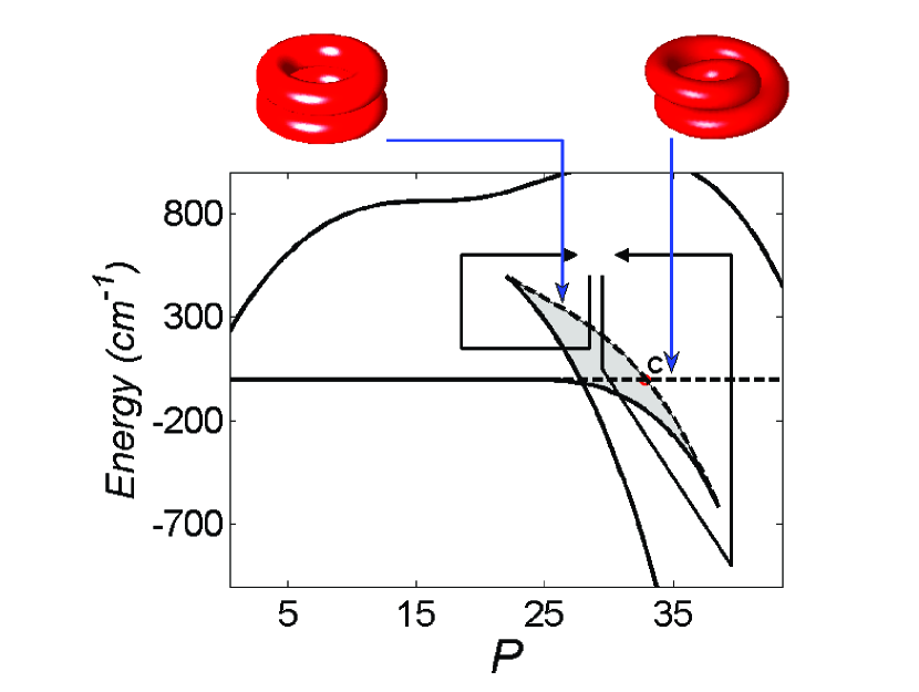
Figure 1: (Color online) Bifurcation diagram of the HOCl molecule for $I_{1}=1/2$ as a function of $P$ [see Eq. (3)]. The energies of the period orbit [B] characterized by $p_{3}=q_{3}=0$ have been subtracted from each energy in order to clarify the plot (see Ref. [15] for details). The critical points of $\mathcal{EM}$ are represented by solid and dashed lines. Points of the solid lines lift to points or circles in the original phase space, while points of the dashed lines lift to curled tori or bitori. A representation of these two singular tori is also given in this figure. The red dot $C$ is the intersection point of these two lines. The two paths with arrows in black correspond to the bipath used to define the bidromy (see the text). The grey region is the zone where the two leaves of the bifurcation diagram overlap.

To better visualize the phenomenon of monodromy, we plot polyads up to $P=44$. $P=38$ is the highest polyad number with an ab initio energy level taken into account in the fit. As can be seen in Fig. 1, the bifurcation diagram has a line of curled tori and a line of bitori which intersect at the point $C$. It is also composed of two leaves, called the upper leaf and the lower one, which overlap in the grey region of the bifurcation diagram. The two leaves are glued together along the singular line of bitori and along the part of the line of curled tori that lies at the right of the point $C$. The other part of the line of curled tori belongs to the upper leaf (see also Fig. 2 which displays the quantum version of this bifurcation diagram).

The vibrational energies can be obtained by a direct quantum computation in each polyad, that is as a function of $P$. However, this calculation is not sufficient to construct the quantum version of the bifurcation diagram and a semi-classical analysis is needed to establish the nature of the classical dynamics associated to each quantum energy level. For that purpose, we introduce the canonical conjugate coordinates $(I_{k},\phi_{k})$ $(k\in\{1,2,3\})$ which are defined by the relations $q_{k}=\sqrt{2I_{k}}\cos\phi_{k}$ and $p_{k}=-\sqrt{2I_{k}}\sin\phi_{k}$. Note that the polar coordinates $(I_{k},\phi_{k})$ are not defined if $p_{k}=q_{k}=0$. The Hamiltonian $H$ can then be expressed in the set of coordinates $(I,\theta)$ and $(J,\psi)$ where $I=2I_{2}+I_{3}$, $J=2I_{2}$, $\theta=\phi_{3}$ and $\psi=\phi_{2}/2-\phi_{3}$ with the constraints $I\geq J$ and $J\geq 0$. The Hamiltonian $H$ is a function of only $I$, $J$ and $\psi$. One of the actions of the system is $I$ which is global and the other one is given by $\mathcal{J}=\int_{\gamma}Jd\psi/(2\pi)$ where the integral is calculated along the projection $\gamma$ of the flow of $H$ on the space $(J,\psi)$. $\mathcal{J}$ depends on the values of $I$ and $E$. The regular Bohr-Sommerfeld rules state that the semi-classical energies are those which satisfy $\mathcal{J}=\hbar(n+1/2)$ and $I=\hbar(P+3/2)$. Knowing the leaf to which the loop $\gamma$ belongs, we associate the same leaf to the corresponding semi-classical energy level. The accuracy of the semi-classical energy levels allows us to do the same for each quantum energy level and to construct the quantum bifurcation diagram. This diagram is displayed in Fig. 2 where we observe in the overlap region of the two leaves a superposition of two lattices of points.
Fractional bidromy. Classical monodromy is the simplest topological obstruction to the existence of global action-angle coordinates [6, 7]. Let us consider the torus-bundle over the regular values of $\mathcal{EM}$. Due to the presence of certain isolated singular tori such as pinched tori, regular tori are forced to fit together with a twist which prevents extending the action-angle variables to the whole bundle. The system has then a non trivial monodromy. From a quantum point of view, we can also analyze the joint spectrum of the corresponding quantum operators and look for the manifestation of classical monodromy in this spectrum [5]. The bifurcation diagram becomes a 2-dimensional lattice of points labeled by the values of the quantum numbers, the energy $E$ and the polyad number $P$ for HOCl. Locally, around a regular value, the lattice is regular in the sense that we can find a map which sends this lattice to $\mathbb{Z}^{2}$. In order to check the global regularity of the spectrum, the method consists in taking a cell, transporting continuously this cell along a closed loop and comparing the final cell with the initial one. If the two cells are different then the system has quantum (or at least semi-classical) monodromy [5].

The theory of Hamiltonian monodromy has known recent important developments, which resulted in the concepts of fractional monodromy [12] and bidromy [13, 14]. These generalizations are associated to particular singular tori, i.e., curled tori for fractional monodromy and bitori for bidromy (see Fig. 1 for a representation of these singular tori), and to loops in the bifurcation diagram which are allowed to cross these lines of singularities. In [12], fractional monodromy characterizes a line of critical values corresponding to curled tori and ended by a point whose preimage is a pinched torus. If we consider loops crossing this line then it can be shown that the notion of Hamiltonian monodromy can still be defined in a restrictive way where the monodromy matrix has fractional coefficients. The bidromy phenomenon was first introduced in a three-degree of freedom system similar to the $\textrm{CO}_{2}$ molecule [13] and exhibited recently in a general class of two-degree of freedom Hamiltonian systems with a bifurcation diagram having a swallowtail structure [14] very close to the one encountered in Fig. 1, except that there is in addition a line of curled tori in Fig. 1. The bidromy matrix is defined through a bipath, i.e., a set of two loops following each a different leaf of the bifurcation diagram. A bipath appears as the only way to generalize the notion of monodromy when the bifurcation diagram has a swallowtail structure and a line of bitori. Note the difference between this case and the standard non local monodromy [8, 2] which is also characterized by a second leaf in the bifurcation diagram but where loops surround the line of bitori without crossing it. As for fractional monodromy, a method to cross unambiguously the line of bitori can be defined. In the quantum version of these generalizations, the size of the fundamental cell has to be increased as discussed below in one of the two directions in order to parallel transport the cell across the line of critical values.

Since the system considered in this paper has both a swallowtail structure and a line of curled tori, we introduce the notion of fractional bidromy which can be viewed as the combination of fractional monodromy and bidromy. As displayed in Fig. 1, we consider a bipath such that one of its two components crosses the line of curled tori. In this example, we restrict the determination of this generalized monodromy to the quantum case.

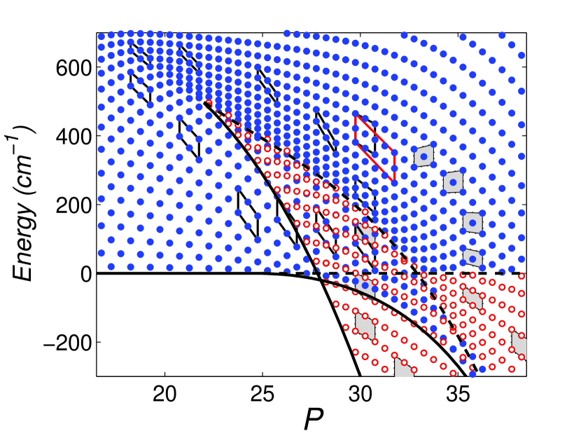
Figure 2: (Color online) Parallel transport of the cell through the vibrational spectrum of HOCl. The energy levels of the upper and lower leaves are respectively depicted in blue (full) and red (open) dots. The effective value of $\hbar$ is taken to be 0.5 for the sake of a clearer illustration. The initial cell is broken into two cells when crossing the line of bitori. One of the two cells, the grey one, belongs to the lower leaf, while the other belongs to the upper leaf. The final cell, the red one, is defined by the addition of the two final cells of the two paths.

Let $u_{1}$ (resp. $v_{1}$) and $u_{2}$ (resp. $v_{2}$) be the two vectors defining the initial (resp. final) cell. The quantum monodromy matrix $M$ is the matrix such that

$$\left(\begin{array}[]{cc}v_{1}\\ v_{2}\end{array}\right)=M\left(\begin{array}[]{cc}u_{1}\\ u_{2}\end{array}\right).$$ (8)

The vectors $u_{2}$ and $v_{2}$ are vertical vectors oriented from the top to the bottom, while the vectors $u_{1}$ and $v_{1}$ are oriented from left to right. To cross the different lines of singularities, the size of the cell has to be increased in the horizontal direction for the line of curled tori [12] and in the vertical direction for the line of bitori [14]. The parallel transport of the cell along the bipath is represented in Fig. 2. The cell is broken into two cells when crossing the line of bitori. The way this line is crossed is not a priori obvious. This parallel transport can be rigorously computed by considering the classical monodromy and its relation with quantum monodromy [14]. After crossing this line of critical values, the two cells are transported along the two parts of the bipath. We finally merge the two final cells by adding their basis vectors, which gives the red cell of Fig. 2. An analysis of Fig. 2 allows to deduce the following relations between the initial and final vectors: $v_{1}=2u_{1}+u_{2}/2$ and $v_{2}=u_{2}$, which leads to the following monodromy matrix $M$:

$$M=\left(\begin{array}[]{cc}2&1/2\\ 0&1\end{array}\right).$$ (11)

Note that the initial vector $u_{1}^{\prime}=u_{1}-u_{2}/2$ is transformed into $2u_{1}^{\prime}$ after one loop, which leads in this case to a diagonal monodromy matrix. If we consider now a bipath crossing the line of bitori at the right of the point $C$ then the same monodromy matrix is obtained although each component of the bipath crosses two times the line of curled tori. This shows that the notion of fractional bidromy is well defined as it does not depend on where the bipath crosses the line of bitori.
Conclusion. This article proposes, to our knowledge, the first example of a molecular system where a generalized monodromy is exhibited. We hope that this example will motivate systematic investigations of generalized monodromy in the rovibronic spectra of resonant molecular systems. Other two degree of freedom molecular systems such as HOBr [16] are expected to present nontrivial generalized monodromies, but this situation is not general. As an example, the bidromy phenomenon does not exist in the HCP molecule [3] since in this case one cannot define a closed bipath turning around the bifurcation points of the bifurcation diagram.

References

- [1] M. Joyeux, S. C. Farantos and R. Schinke, J. Phys. Chem. A 106, 5407 (2002); B. I. Zhilinskií, Phys. Rep. 341, 85 (2001).
- [2] M. S. Child, Adv. Chem. Phys. 136 (2007).
- [3] M. Joyeux, D. Sugny, V. Tyng, M. E. Kellman, H. Ishikawa, R. W. Field, C. Beck and R. Schinke, J. Chem. Phys. 122, 4162 (2000); G. Michalski, R. Jost, D. Sugny, M. Joyeux and M. Thiemens, J. Chem. Phys. 121, 7153 (2004).
- [4] M. Joyeux and D. Sugny, Can. J. Phys. 80, 1459 (2002).
- [5] S. V. Ngoc, Comm. Math. Phys. 203, 465 (1999).
- [6] J. J. Duistermaat, Commun. Pure Appl. Math. 33, 687 (1980).
- [7] R. H. Cushman and L. Bates, Global Aspects of Classical Integrable Systems, Birkhauser, Basel (1997).
- [8] K. Efstathiou, Metamorphoses of Hamiltonian Systems with Symmetry (Springer-Verlag, Lecture Notes in Mathematics 1864, Heidelberg, 2005).
- [9] D. A. Sadovskií and R. H. Cushman, Physica D 142, 166 (2000); I. N. Kozin and R. M. Roberts, J. Chem. Phys. 118, 10523 (2003); H. Waalkens, A. Junge and H. R. Dullin, J. Phys. A 36, L307 (2003); K. Efstathiou, M. Joyeux and D. A. Sadovskií, Phys. Rev. A 69, 032504 (2004); R. H. Cushman, H. R. Dullin, A. Giacobbe, D. D. Holm, M. Joyeux, P. Lynch, D. A. Sadovskií and B. I. Zhilinskií, Phys. Rev. Lett. 93, 024302 (2004).
- [10] N. J. Fitch, C. A. Weidner, L. P. Parazzoli, H. R. Dullin and H. J. Lewandowski, Phys. Rev. Lett. 103, 034301 (2009); H. R. Dullin and H. Waalkens, Phys. Rev. Lett. 101, 070405 (2008).
- [11] C. D. Cooper and M. S. Child, Phys. Chem. Chem. Phys. 7, 2731 (2005).
- [12] N. N. Nekhoroshev, D. A. Sadovskií and B. I. Zhilinskií, Ann. H. Poincaré 7(6), 1099 (2006); D. Sugny, P. Mardesic, M. Pelletier, A. Jebrane and H. R. Jauslin, J. Math. Phys. 49, 042701 (2008).
- [13] D. A. Sadovskií and B. I. Zhilinskií, Ann. of Physics 322, 164 (2007).
- [14] K. Efstathiou and D. Sugny, J. Phys. A 43, 085216 (2010).
- [15] R. Jost, M. Joyeux, S. Sokov and J. Bowman, J. Chem. Phys. 111, 6807 (1999); note two misprints: the correct coefficients are and .
- [16] T. Azzam, R. Schinke, S. C. Farantos, M. Joyeux and K. A. Peterson, J. Chem. Phys. 118, 9643 (2003).