Ball on a Beam: Stabilization under Saturated Input Control with Large Basin of Attraction

Abstract

This article is devoted to the stabilization of two under actuated planar systems, the well known straight beam-and-ball system and an original circular beam-and-ball system. The feedback control for each system is designed, using the Jordan form of its model, linearized near the unstable equilibrium. The limits on the voltage, fed to the motor, are taken into account explicitly. The straight beam-and-ball system has one unstable mode in the motion near the equilibrium point. The proposed control law ensures that the basin of attraction coincides with the controllability domain. The circular beam-and-ball system has two unstable modes near the equilibrium point. Therefore this device, never considered in the past, is much more difficult to control than the straight beam-and-ball system. The main contribution is to propose a simple new control law, which ensures, by adjusting its gain parameters, that the basin of attraction arbitrarily can approach the controllability domain for the linear case. For both nonlinear systems, simulation results are presented to illustrate the efficiency of the designed nonlinear control laws and to determine the basin of attraction.

saturated control, controllability domain, Jordan form, stabilization, basin of attraction.

1 Introduction

Among the mechanical systems, the under actuated systems, which have fewer controls than configuration variables, represent a great challenge for the control. They are characterized by the underactuation degree, which is the difference between the numbers of configuration variables and controls. An active field of research exists, due to the applications of under actuated systems such as aircrafts, satellites with thrusters, spacecrafts, flexible robots, legged robots, which adopt a dynamical stable walking or running gait, inverted pendulums. For example, for a planar vertical take-off and landing aircraft (PVTOL), an approximate input-output linearization procedure is developed in Hauser92 to get a bounded tracking and an asymptotic stability. In paper alimir03 , the stabilization of a satellite is studied when one of its three thrusters is not efficient. Flexible robots have an infinite number of flexible modes, which can be damped, using a controller, based on a discrete model, (see Book83 , DeLuca91 , etc…). Inverted pendulum devices are used like a testbed research or for education application to investigate new control laws for the stabilization or the swing up (see Astrom00 , grishin02 or spong95 ). Mechanical models of two planar systems, which have an unactuated cyclic variable, and all their shape variables are independently actuated, are considered in GrizzleMoChe05 . To deal with the stability of a walking gait for a biped, which is under actuated in single support, because it has point feet, in the papers Aoustin991 , Aoustin031 and Plestan03 , reference trajectories are defined for the actuated variables as functions of an undriven strictly monotone state variable. A complete characterization of all mechanical systems with underaction degree one is given in Acosta04 . In Fantoni02 , a control law is proposed to stabilize the surge, sway and angular velocities of the hovercraft system. We can also note the very interesting thesis document Saber010 , which is devoted to nonlinear control, reduction, and classification of under actuated mechanical systems and in particular of high order under actuated systems. Then numerous mechanical devices associated with underactuation have been studied in literature. Furthermore this topic is far to be closed, because control design methods do not exist for many under actuated systems that are important for applications.

This paper deals with the stabilization of two planar under actuated systems. The first system is the well-known straight beam-and-ball system. The ball is perfectly rolling without slide on the beam. Due to the complexity of this system, the stabilization and the tracking problem using a state or an output feedback have been considered by many researchers (see Hauser92_bis , TeelPraly95 , Tellistambul92 , SepJanKok97 or Saber010 ). In paper Hauser92_bis , tracking for this system was considered using approximate input-output linearization. Semiglobal stabilization of the straight beam-and-ball system using state feedback was addressed by Tellistambul92 . In TeelPraly95 , this system is stabilized using output feedback. The problem of global stabilization of the straight beam-and-ball system with friction was considered in paper SepJanKok97 . The viscous friction is taken into account in our paper too. Semiglobal stabilization of this system, using fixed-point state feedback was addressed by Saber010 .

The second system is an original circular beam-and-ball system. For each system, a control law, based on the linearized model and its Jordan form is designed. The saturation of the actuator is taken into account explicitly, so the control law is non-linear. This kind of control has been previously tested to stabilize a biped with point feet Aoustin043 , a one-link pendulum with flywheel grishin02 , and to stabilize a two-link pendulum with flywheel Aoustin061 . The main difference between the straight beam-and-ball system and the circular beam-and-ball system is that the linear model of the second system has two eigenvalues in the right-half complex plane. Therefore, it is more difficult to stabilize the circular beam-and-ball system than the straight beam-and-ball system with only one eigenvalue in the right-half complex plane. For the linearized model of the straight beam-and-ball system, the controllability domain, noted $Q$, and the basin of attraction, noted $B$, can coincide under a linear control law with restriction (see formal74 , grishin02 ). This property is not satisfied for the linearized model of the circular beam-and-ball system with two eigenvalues in the right-half complex plane. But the basin of attraction $B$ can be made arbitrary close to the controllability domain $Q$ (see HuLinQiu01 ).

We hope that our study is of theoretical interest and also has some pedagogical value.

The paper is organized as follows: Section 2 is devoted to the straight beam-and-ball system. In Subsection 2.1, the equations of motion are written. The linear model is presented in Subsection 2.2. Subsections 2.3, 2.4, 2.5 are organized to introduce a control law with saturation, to get a basin of attraction $B$, which coincides with the controllability domain $Q$. The circular beam-and-ball system is studied in Section 3. In Subsection 3.1, the equations of motion are written. The linear model is presented in Subsection 3.2. Subsections 3.3, 3.4, 3.5 are organized to introduce a control law with saturation, to get a large basin of attraction $B$ inside the controllability domain $Q$. Simulation results for the complete nonlinear systems are shown to illustrate the efficiency of the proposed control laws. Finally, Section 4 contains our conclusion and perspectives.

2 Straight beam-and-ball system

The straight beam-and-ball system consists of a straight beam and a ball on it, see Figure 1. The ball is rolling on the beam without slide. The point $C_{1}$ is center of mass of the beam with its holder $OA$. The point $C_{2}$ and and value $r$ are center and radius of the ball. The point $C_{2}$ is also the center of mass of the ball.

2.1 Equations of motion

Let $m_{1}$ and $m_{2}$ denote the mass of the beam with its holder $OA$ and the mass of the ball, respectively. Let us introduce $\rho_{1}$ and $\rho_{2}$ the radii of inertia such that $I_{1}=m_{1}\rho_{1}^{2}$ and $I_{2}=m_{2}\rho_{2}^{2}$ are respectively the inertia moment of the beam with its holder $OA$ around the suspension point $O$ and the inertia moment of the ball around its center $C_{2}$; let $OC_{1}=a$ and $OA=l$.

Two generalized coordinates, the angular variables $\theta$ and $\varphi$ characterize the behavior of this system. Position of the ball on the beam is defined also by the distance $s=r\varphi$. Let $\Gamma$ be the torque, which is directly proportional to the electrical current in the armature winding. By neglecting the armature inductance (in other words, the electromagnetic time constant in the rotor circuit), this torque can be written in the form (see Gorinevsky97 ):

$$\Gamma=c_{u}u-c_{v}\dot{\theta}$$ (1)

where $u$ is the voltage, supplied to the motor. The positive constants $c_{u}$ and $c_{v}$ for a given motor can be calculated by using the values for the starting torque, the nominal voltage, the nominal torque and the nominal angular velocity Gorinevsky97 . Product $c_{v}\dot{\theta}$ is the torque of the back electromotive force. The torque of the viscous friction force in the joint $O$ (if it is taken into account) is also proportional to angular velocity $\dot{\theta}$. We will consider the following constraint, imposed on the voltage $u$:

$$|u|\,\leq\,u_{0},\,\thinspace\thinspace u_{0}\,=\,const$$ (2)

The expressions for the kinetic energy $K$ and the potential energy $\Pi$ are the following ($g$ is the gravity acceleration):

$$\begin{array}[]{c}2K=m_{1}\rho_{1}^{2}\dot{\theta}^{2}+m_{2}[r^{2}\varphi^{2}+(r+l)^{2}]\dot{\theta}^{2}+2m_{2}r(l+r)\dot{\varphi}\dot{\theta}+m_{2}(r^{2}+\rho_{2}^{2})\dot{\varphi}^{2}\\ \\ \Pi=m_{1}gacos\theta+m_{2}g[-r\varphi sin\theta+(l+r)cos\theta]\end{array}$$ (3)

The equations of the mechanism motion can be derived, using Lagrange’s method:

$$\begin{array}[]{c}\left[m_{1}\rho_{1}^{2}+m_{2}(r+l)^{2}+m_{2}r^{2}\varphi^{2}\right]\ddot{\theta}+m_{2}r(r+l)\ddot{\varphi}+2m_{2}r^{2}\varphi\dot{\varphi}\dot{\theta}-\\ -g[m_{1}a+m_{2}(r+l)]sin\theta-m_{2}gr\varphi cos\theta=c_{u}u-c_{v}\dot{\theta}\end{array}$$ (4)

$$r(r+l)\ddot{\theta}+(r^{2}+\rho_{2}^{2})\ddot{\varphi}-r^{2}\varphi\dot{\theta}^{2}-grsin\theta=0$$ (5)

If $u=0$, system (4), (5) has one unstable equilibrium state:

$$\theta=0,\quad\varphi=0\quad(s=0),\quad\dot{\theta}=0,\quad\dot{\varphi}=0\quad(\dot{s}=0)$$ (6)

2.2 Linearized Model

Corresponding to the nonlinear equations (4), (5), the linear model of the motion near the unstable equilibrium state (6) is:

$$\left[m_{1}\rho_{1}^{2}+m_{2}(r+l)^{2}\right]\ddot{\theta}+m_{2}r(r+l)\ddot{\varphi}-g[m_{1}a+m_{2}(r+l)]\theta-m_{2}gr\varphi=c_{u}u-c_{v}\dot{\theta}\\$$ (7)

$$r(r+l)\ddot{\theta}+(r^{2}+\rho_{2}^{2})\ddot{\varphi}-gr\theta=0$$ (8)

2.3 Kalman controllability

The determinant of the controllability matrix (see kalman69 ) for the linear model (7), (8) is not null, if and only if:

$$r^{2}g^{2}\left[(2r^{2}+\rho_{2}^{2})\rho_{2}^{2}+r^{4}\right]\neq 0$$ (9)

Thus, inequality (9) is valid, if $r\neq 0$. If $r=0$, then the ball becomes a material point and we do not consider this case. Thus, the linear model of the straight beam-and-ball system is always controllable.

2.4 Spectrum of Linear System

The state form of system (7), (8), using the state vector $x=(\theta,~{}\varphi,~{}\dot{\theta},~{}\dot{\varphi})^{T}$, is:

$$\dot{x}=Ax+bu=\left[\begin{array}[]{cc}0_{2\times 2}{}&~{}I_{2\times 2}\\ \\ D^{-1}E{}&~{}D^{-1}\left(\begin{array}[]{cc}-c_{v}&0\\ 0&0\\ \end{array}\right)\end{array}\right]x+\left[\begin{array}[]{c}0\\ 0\\ D^{-1}\left(\begin{array}[]{c}c_{u}\\ 0\\ \end{array}\right)\\ \end{array}\right]u$$ (10)

The notations $0_{2\times 2}$ and $I_{2\times 2}$ define a zero matrix and an identity matrix, respectively. The expressions of matrices $D$ and $E$ are

$$\begin{array}[]{c}D=\left(\begin{array}[]{cc}m_{1}\rho_{1}^{2}+m_{2}(r+l)^{2}{}&~{}m_{2}r(r+l)\\ r(r+l){}&~{}r^{2}+\rho_{2}^{2}\\ \end{array}\right)\\ \\ E=g\left(\begin{array}[]{cc}m_{1}a+m_{2}(r+l){}&~{}m_{2}r\\ r{}&~{}0\\ \end{array}\right)\end{array}$$ (11)

Introducing a nondegenerate linear transformation $x=Sy$ with a constant matrix $S$, it is possible to get the well-known Jordan form of the matrix equation (10)

$$\dot{y}=\Lambda y+du$$ (12)

where

$$\begin{array}[]{c}\Lambda=S^{-1}AS=\left(\begin{array}[]{ccccc}\lambda_{1}&&&0\\ &\lambda_{2}&&\\ &&\lambda_{3}&\\ 0&&&\lambda_{4}\\ \end{array}\right),\quad d=S^{-1}b=[d_{i}]^{T}\,\quad(i=1,...,4).\\ \end{array}$$ (13)

Here, $\lambda_{1},...,\lambda_{4}$ are the eigenvalues of the matrix $A$. They are the roots of the characteristic equation of system (7), (8):

$$a_{0}\lambda^{4}+a_{1}\lambda^{3}+a_{2}\lambda^{2}+a_{3}\lambda+a_{4}=0$$ (14)

with

$a_{0}=detD>0,\quad a_{1}=c_{v}(r^{2}+\rho_{2}^{2})>0,\quad a_{2}=m_{2}(r+l)(r^{2}-\rho_{2}^{2})-m_{1}a(r^{2}+\rho_{2}^{2}),\\ \\ a_{3}=0$, $a_{4}=detE=-m_{2}g^{2}r^{2}<0.\\ \\$ If all physical parameters of the studied system are known, matrix $S$ of the transformation $x=Sy$ can be calculated.

According to the theorem of Routh-Hurwitz (see GraninoTheresa68 ), equation (14) has one root in the right-half complex plane and three roots in the left-half complex plane (see also Saber010 ). This assertion does not depend on the sign of the coefficient $a_{2}$. Of course, the unique root in the right-half complex plane is located on the real axis.

In Section 3, we consider the ball on the circular beam and use linearized model in the same matrix form (10) as for the ball on the straight beam, but with different submatrices $D$ and $E$.

2.5 Problem Statement

Let $x=0$ (here $0$ is a ($4\times 1$) zero-column) be the desired equilibrium state of system (10). Let us design the feedback control $u(x)$ to stabilize this equilibrium state $x=0$, under constraint (2). In other words, we want to design an admissible (satisfying the inequality (2)) feedback control $|u(x)|\leq u_{0}$ to ensure the asymptotic stability of the desired state $x=0$. Let $W$ be the set of piecewise continuous functions of time $u(t)$, satisfying inequality (2). Let $Q$ be the set of the initial states $x(0)$ of system (10), from which origin $x=0$ can be reached, using admissible control functions of time $u(t)$. In other words, system (10) can reach the origin $x=0$ with the control $u(t)\,\in\,W$, only starting from the initial states $x(0)\,\in\,Q$. Set $Q$ is called controllability domain. If the matrix $A$ has eigenvalues with positive real parts and the control variable $u$ is restricted, then the controllability domain $Q$ for system (10) is an open subset of the phase space $X$ (see formal74 , grishin02 ).

For any admissible feedback control $u=u(x)$ with saturation $|u(x)|\,\leq\,u_{0}$ the corresponding basin of attraction belongs to the controllability domain: $B\subset Q$. Here, as usual, $B$ is the set of initial states $x(0)$, from which system (10), with feedback $u=u(x)$ asymptotically tends to the origin point $x=0$ as $t\rightarrow\infty$.

In the following section, a control law will be presented for the straight beam-and-ball system to get a basin of attraction $B$, which coincides with the controllability domain $Q$: $B=Q$.

2.6 Feedback Control for the straight beam-and-ball system

A control law is proposed here to stabilize the straight beam-and-ball system with basin of attraction as large as possible.

2.6.1 Control design

Let $\lambda_{1}$ be the real positive eigenvalue, $Re\lambda_{i}<0$ ($i=2,~{}3,~{}4$) and let us consider the first scalar differential equation of system (12) corresponding to eigenvalue $\lambda_{1}$,

$$\dot{y}_{1}=\lambda_{1}y_{1}+d_{1}u$$ (15)

System (10), is a Kalman controllable system, therefore scalar $d_{1}\neq 0$. The controllability domain $Q$ of the equation (15) and consequently of system (12) is described by the following inequality (see formal74 , grishin02 )

$$\left|y_{1}\right|<\left|d_{1}\right|\frac{u_{0}}{\lambda_{1}}$$ (16)

The instability of the coordinate $y_{1}$ can be “suppressed” by a linear feedback control,

$$u=\gamma y_{1}$$ (17)

with the following condition,

$$\lambda_{1}+d_{1}\gamma\,<\,0$$ (18)

For system (10) under the feedback control (17) with inequality (18), only the pole $\lambda_{1}$ is replaced by a negative pole $\lambda_{1}+d_{1}\gamma$. The poles $\lambda_{2}$, $\lambda_{3}$, $\lambda_{4}$ do not change.

If constraint (2) is taken into account, the linear feedback control (17) becomes with saturation,

$$u=u(y_{1})=\left\{\begin{array}[]{rlll}u_{0},&\quad if&\gamma y_{1}\geq u_{0}&\\ \\ \gamma y_{1},&\quad if&|\gamma y_{1}|\leq u_{0}&\\ \\ -u_{0},&\quad if&\gamma y_{1}\leq-u_{0}&\\ \end{array}\right.$$ (19)

The unit of coefficient $\gamma$ is volt.

It is possible to see that if $|y_{1}|<|d_{1}|u_{0}/\lambda_{1}$, then under condition (18) the right part of equation (15) with the nonlinear control (19) is negative when $y_{1}>0$ and positive when $y_{1}<0$. Consequently, if $|y_{1}(0)|<|d_{1}|u_{0}/\lambda_{1}$, then the solution $y_{1}(t)$ of system (15), (19) tends to 0 as $t\rightarrow\infty$. But if $y_{1}(t)\rightarrow 0$, therefore, according to expression (19), $u(t)\rightarrow 0$ as $t\rightarrow\infty$. Therefore, the solutions $y_{i}(t)$ ($i=2,3,4$) of the second, third and fourth equations of system (12) with any initial conditions $y_{i}(0)$ ($i=2,3,4$) converge to zero as $t\rightarrow\infty$, because $Re\lambda_{i}<0$ for $i=2,3,4$. Thus, under the nonlinear control (19) and with inequality (18), the basin of attraction $B$ coincides with the controllability domain $Q$ (see formal74 , grishin02 ): $B=Q$. So, the basin of attraction $B$ for system (10), (19) is as large as possible and it is described by inequality (16).

Note that the variable $y_{1}$ depends on the original variables from the vector $x$, according to the transformation $x=Sy$ or $y=S^{-1}x$. Due to this, formula (19) defines the control feedback, which depends on the vector $x$ of the original variables. If the matrix $S$ is calculated, then all coefficients of the designed control can be defined. Only the constant $\gamma$ is an arbitrary multiplier, but it has to satisfy inequality (18)

Thus, linearizing nonlinear system (4), (5), (19) near the equilibrium state we obtain a system, which is asymptotically stable. Using Lyapounov’s theorem (see KHALIL02 ), we conclude that equilibrium (6) of the nonlinear system (4), (5) is asymptotically stable under control (19) with some basin of attraction. In the next Subsection, numerically we find the upper bounds of the initial values of some variables, which can be handled for the linear and nonlinear models under the designed control.

2.6.2 Numerical results

Let

$$\begin{array}[]{c}m_{1}=1.0\thinspace kg,\quad m_{2}=0.2\thinspace kg,\quad g=9.81\thinspace m/s^{2},\\ \\ r=0.05\thinspace m,\quad l=0.2\thinspace m,\quad a=0.15\thinspace m,\quad\rho_{1}=0.2179\thinspace m,\quad\rho_{2}=0.1414\thinspace m,\thinspace\\ \\ c_{u}=0.007\thinspace N\raisebox{2.27626pt}{.}m/V,\quad c_{v}=0.0001\thinspace N\raisebox{2.27626pt}{.}m/s,\quad u_{0}=19\thinspace V.\\ \end{array}$$ (20)

In open-loop the poles of the linear system (10) (the roots of equation (14)) with parameters (20) are:

$$\lambda_{1}=5.7202,\quad\lambda_{2}=-5.7218,\quad\lambda_{3},\lambda_{4}=-2.8\raisebox{2.27626pt}{.}10^{-7}\pm 1.0558i,\quad\\$$ (21)

Now we can use inequality (16) to evaluate the basin of attraction $B$ for system (10), (19). If $\theta(0)=\dot{\theta}(0)=\dot{\varphi}(0)=0$, the upper bound of the initial angles $\varphi$, which can be handled for the linear model (10) is $\varphi(0)\cong 77.679\textdegree$. The corresponding initial distance $s(0)$ is equal to $0.0678~{}m$. This value for the distance $s$ is close to the value

$$s(0)=\frac{c_{u}u_{0}}{m_{2}g}$$ (22)

With $\theta=0$ product $sm_{2}g$ is the torque about joint O of the gravity force of the ball (see the nonlinear equations (4), (5) and the linear equations (7), (8)), the product $c_{u}u_{0}$ is the torque (maximal as possible) developed by the motor in static. Thus, the point

$$\theta=\dot{\theta}=\dot{s}=0,\quad s=\frac{c_{u}u_{0}}{m_{2}g}$$ (23)

is the equilibrium state (unstable) for our system (nonlinear (4), (5) and linear (7), (8)). It is easily to see that the equilibrium point (23) is located on the boundary of the controllability region (16). Simulation shows that, if

$$\theta(0)=\dot{\theta}(0)=\dot{s}(0)=0,\quad s(0)\geq\frac{c_{u}u_{0}}{m_{2}g},$$ (24)

then it is not possible to bring the nonlinear system (4), (5) under control (19) to the equilibrium (6); but it is possible to do that, if $s(0)<\frac{c_{u}u_{0}}{m_{2}g}$. Furthermore, we think there is no an admissible control $|u(x)|\leq u_{0}$ to bring system (4), (5) to the equilibrium point (6) from the initial states (24). This opinion is based on the numerical studies and physical feeling. We do not prove here corresponding assertion strictly.

The eigenvalues $\lambda_{3}$, $\lambda_{4}$ are very close to the imaginary axis (see (21)) and therefore under the control (19), the transient process is very long. Let us take into account a viscous friction in the joint $O$ defined by the torque $f\dot{\theta}$. The consideration of the torque $f\dot{\theta}$ of the friction force is equivalent to the consideration in equation (1) of the term $(c_{v}+f)\dot{\theta}$ instead of the term $c_{v}\dot{\theta}$. With $f=0.4~{}N\raisebox{2.27626pt}{.}m\raisebox{2.27626pt}{.}s$ for example the poles of the corresponding linear system (10) in open-loop are:

$$\lambda_{1}=3.4001,\quad\lambda_{2}=-10.0181,\quad\lambda_{3},\lambda_{4}=-0.1041\pm 1.0297i\\$$ (25)

The technique of the feedback control design with a viscous friction (with new poles (25)) remains the same exactly. And the structure of this control remains the same - (19). Under the control law (19) with new coefficients, the transient process converges to the equilibrium state (6) faster than without friction. Using inequality (16), or the equality (22) we get of course the same value $s(0)$ as above without friction. So, we can use formula (22) for the linear and nonlinear systems to calculate the upper bound of the initial distances $s$, which are possible to stabilize the equilibrium state (6).

Figures 2 and 3 show a numerical test with an initial tilt $\varphi(0)=77.65\textdegree$ for the nonlinear system (4), (5) with the coefficient $f=0.4~{}N\raisebox{2.27626pt}{.}m\raisebox{2.27626pt}{.}s$ under the control law (19) with $\gamma=-122$. The voltage, supplied to the motor, is shown in Figure 3. The limit value $u_{0}=-19~{}V$ is reached at initial time.

Let $F$ be the reaction force, applied to the ball orthogonally to the beam in their contact point. The following formula for this force holds:

$$F=m_{2}\left[g~{}cos\theta-(l+r)\dot{\theta}^{2}-2r\dot{\varphi}\dot{\theta}-r\varphi\ddot{\theta}\right]$$ (26)

If the reaction force $F$ becomes negative, then the ball loses contact with the beam and our model (with contact) becomes false to describe the physical process. In the numerical experiment, presented in Figures 2 and 3, the force $F$ is always positive. This force is shown in Figure 4.

If $\varphi(0)=\dot{\varphi}(0)=\dot{\theta}(0)=0$, then, using inequality (16), the upper bound of the initial tilts of the beam, which can be handled, for the linear model (10) with the friction is $\theta(0)=3.61\textdegree$. The computations show that the upper bound of the initial tilts for the nonlinear system (4), (5) under control (19) is $\theta(0)=3.64\textdegree$. So, this value is little more important than for the linear system (10) under the same control (19).

3 Circular beam-and-ball system

The circular beam-and-ball system consists of a circular beam with the center $C$ and the radius $R$ and a ball on it with the center $C_{2}$ and the radius $r$, see Figure 5. The point $C_{1}$ is the center of mass of the beam with its holder $OA$.

3.1 Equations of motion

Here the same notations are used, that for the straight beam-and-ball system.

Let $m_{1}$ and $m_{2}$ denote the mass of the beam with its holder $OA$ and the mass of the ball, respectively. Let $\rho_{1}$ and $\rho_{2}$ be the radii of inertia respectively of the beam with its holder $OA$ and of the ball; let $OC_{1}=a$ and $OA=l$ be.

The generalized coordinates are the joint variable $\theta$ and the angle variable $\varphi$. Position of the ball on the beam is also defined by distance $s=r\varphi$. The relation between the angle $\varphi$ and angle $\psi$ is:

$$r\varphi=R\psi$$

Let us assume that the motor is the same that for the straight beam-and-ball system with torque (1) and constraint (2). The constants $c_{u}$, $c_{v}$ and $u_{0}$ are the same.

The expressions for the kinetic energy $K$ and the potential energy $\Pi$ are the following:

$$\begin{array}[]{c}2K=\left\{m_{1}\rho_{1}^{2}+m_{2}\left[(R+r)^{2}+(l-R)^{2}+2(R+r)(l-R)cos\frac{r\varphi}{R}\right]\right\}\dot{\theta}^{2}+\\ +m_{2}\left[(R+r)^{2}+\frac{(\rho_{2}R)^{2}}{r^{2}}\right]\frac{(r\dot{\varphi})^{2}}{R^{2}}+\\ +2m_{2}\left[(R+r)^{2}+(R+r)(l-R)cos\frac{r\varphi}{R}\right]\dot{\theta}\frac{r\dot{\varphi}}{R}\\ \\ \Pi=[m_{1}a+m_{2}(l-R)]gcos\theta+m_{2}g(R+r)cos(\frac{r}{R}\varphi+\theta)\end{array}$$ (27)

The equations of the mechanism motion are derived, using Lagrange’s method:

$$\begin{array}[]{c}\left[m_{1}\rho_{1}^{2}+m_{2}(r^{2}+l^{2}+2rlcos\frac{r\varphi}{R})+2m_{2}R(R+r-l)(1-cos\frac{r\varphi}{R})\right]\thinspace\ddot{\theta}+\\ \\ +m_{2}r(1+\frac{r}{R})\left[R+r+(l-R)cos\frac{r\varphi}{R}\right]\thinspace\ddot{\varphi}+m_{2}r(1+\frac{r}{R})(R-l)(2\dot{\theta}+\frac{r\dot{\varphi}}{R})\dot{\varphi}sin\frac{r\varphi}{R}-\\ \\ -g[m_{1}a\thinspace+m_{2}(l-R)]sin\theta-m_{2}g(R+r)sin(\theta+\frac{r\varphi}{R})=c_{u}u-c_{v}\dot{\theta}\end{array}$$ (28)

$$\begin{array}[]{c}r(1+\frac{r}{R})\left[R+r+(l-R)cos\frac{r\varphi}{R}\right]\thinspace\ddot{\theta}+\left[\rho_{2}^{2}+r^{2}(1+\frac{r}{R})^{2}\right]\thinspace\ddot{\varphi}+\\ \\ +(1+\frac{r}{R})(l-R)\dot{\theta}^{2}sin\frac{r\varphi}{R}-gr(1+\frac{r}{R})sin(\theta+\frac{r\varphi}{R})=0\end{array}$$ (29)

If $u=0$, system (28), (29) has one unstable equilibrium state (6).

3.2 Linearized Model

Linearizing the equations (28), (29) near the unstable equilibrium state (6), we get the following model:

$$\begin{array}[]{c}\left[m_{1}\rho_{1}^{2}+m_{2}(r+l)^{2}\right]\ddot{\theta}++m_{2}r\left(1+\frac{r}{R}\right)(r+l)\ddot{\varphi}-\\ \\ -g[m_{1}a+m_{2}(r+l)]\theta-m_{2}g(r+R)\frac{r\varphi}{R}=c_{u}u-c_{v}\dot{\theta}\end{array}$$ (30)

$$\begin{array}[]{c}r\left(1+\frac{r}{R}\right)(r+l)\thinspace\ddot{\theta}+\left[\rho_{2}^{2}+r^{2}\left(1+\frac{r}{R}\right)^{2}\right]\thinspace\ddot{\varphi}-gr\left(1+\frac{r}{R}\right)\left(\theta+\frac{r\varphi}{R}\right)=0\end{array}$$ (31)

3.3 Kalman controllability

The determinant of the controllability matrix for the model (30), (31) is not null, if and only if:

$$Rr^{2}(R-l)+R^{2}\rho_{2}^{2}+r^{3}(R-l)\neq 0$$ (32)

If $r=0$, then the ball becomes a material point and $\rho_{2}=0$. In this case, instead of inequality (32) the equality is correct. However, we do not consider a material point on the beam and therefore assume $r\neq 0$.

Let $r\neq 0$, but the mass of the ball is concentrated in its center $(\rho_{2}=0)$ and the suspension point $O$ coincides with the curvature center $C$ of the circular beam ($R=l$). In this case, inequality (32) is not satisfied and the linear system is not controllable. Consider the controllability of the original nonlinear system (28), (29) in the case $\rho_{2}=0$ and $R=l$. Introduce the angle $\alpha=\theta+\frac{r\varphi}{R}$. The nonlinear system (28), (29) becomes:

$$\begin{array}[]{c}m_{1}\rho_{1}^{2}\ddot{\theta}-m_{1}gasin\theta=c_{u}u-c_{v}\dot{\theta}\end{array}$$ (33)

$$(R+r)\ddot{\alpha}-gsin\alpha=0$$ (34)

The equations (33) and (34) are separated. The control $u$ has no action on the angle $\alpha$ and system (33), (34) is not controllable.

Inequality (32) is satisfied, if

$$l-R\neq\frac{R^{2}\rho_{2}^{2}}{(R+r)r^{2}}$$ (35)

and we will consider only this case.

3.4 Spectrum of Linear System

The state form of system (30), (31) can be presented in the same matrix form (10) as for the straight beam, but with the following submatrices $D$ and $E$:

$$\begin{array}[]{c}D=\left(\begin{array}[]{cc}m_{1}\rho_{1}^{2}+m_{2}(r+l)^{2}{}&~{}m_{2}r(1+\frac{r}{R})(r+l)\\ \\ r(1+\frac{r}{R})(r+l){}&~{}\rho_{2}^{2}+r^{2}(1+\frac{r}{R})^{2}\\ \end{array}\right)\\ \\ E=g\left(\begin{array}[]{cc}m_{1}a+m_{2}(r+l){}&~{}m_{2}r(1+\frac{r}{R})\\ \\ r(1+\frac{r}{R}){}&~{}r(1+\frac{r}{R})\frac{r}{R}\\ \end{array}\right)\end{array}$$ (36)

Introducing a nondegenerate linear transformation $x=Sy$ with a constant matrix $S$, we can get the Jordan form similar to (12), (13).

The characteristic equation of system (30), (31) has form (14) with

$a_{0}=detD>0,\quad a_{1}=c_{v}\left[\rho_{2}^{2}+\frac{r^{2}}{R^{2}}(R+r)^{2}\right]>0,\quad\\ \\ a_{2}=-m_{1}g\left[(\rho_{2}^{2}+r^{2})aR^{2}+(2ar+\rho_{1}^{2})Rr^{2}+(ar+\rho_{1}^{2})r^{3}\right]-\\ \\ ~{}~{}~{}~{}~{}~{}~{}-m_{2}g\left[(r+l)R^{2}(r^{2}-\rho_{2}^{2})+(r^{2}-l^{2})r^{2}R-(r+l)lr^{3}\right],\\ \\ a_{3}=-c_{v}g\frac{r^{2}}{R^{2}}(R+r)<0,\quad$ $a_{4}=detE=g^{2}\frac{r^{2}}{R^{2}}(R+r)[m_{1}a+m_{2}(l-R)].\\$

We assume that

$$m_{1}a+m_{2}(l-R)>0$$ (37)

Inequality (37) is satisfied, if the radius $R$ of the circular beam is sufficiently small (the curvature of the beam is sufficiently large). But we have not to forget condition (32) (or (35)) of controllability.

Under condition (37), the coefficient $a_{4}$ is positive. Using the theorem of Routh-Hurwitz (see GraninoTheresa68 ), we can conclude that the characteristic equation (14) has two roots in the right-half complex plane and two roots in the left-half complex plane. This conclusion does not depend on the sign of the coefficient $a_{2}$.

3.5 Problem Statement

We will consider the same problem, as before for the straight beam-and-ball system. We want to design an admissible (satisfying inequality (2)) feedback control to ensure the asymptotic stability of the state $x=0$ with a large basin of attraction for this equilibrium state.

3.6 Feedback control for the circular beam-and-ball system

A feedback control law $u(x)$, satisfying inequality (2), is proposed here to stabilize the circular beam-and-ball system with a large basin of attraction. Under condition (37), the linear model of the system has two eigenvalues $\lambda_{1}$, $\lambda_{2}$ in the right-half complex plane and two eigenvalues $\lambda_{3}$, $\lambda_{4}$ in the left-half complex plane.

3.6.1 Control design

Let $\lambda_{1}$ and $\lambda_{2}$ be the real positive eigenvalues, and let us consider the first two scalar differential equations of system (12), (13) for the circular beam, corresponding to these eigenvalues $\lambda_{1}$ and $\lambda_{2}$:

$$\dot{y}_{1}=\lambda_{1}y_{1}+d_{1}u,\quad\dot{y}_{2}=\lambda_{2}y_{2}+d_{2}u$$ (38)

Under condition (35) system (10) for the circular beam is Kalman controllable. Therefore, subsystem (38) is controllable too (see kalman69 ) and $d_{1}\neq 0$, $d_{2}\neq 0$. The controllability domain $Q$ of the equations (38), and consequently of system (12), is an open bounded set with the following boundaries (see Boltyansky66 )

$$\begin{array}[]{l}y_{1}(\tau)=\pm\frac{d_{1}u_{0}}{\lambda_{1}}\left(2e^{-\lambda_{1}\tau}-1\right),\\ \\ y_{2}(\tau)=\pm\frac{d_{2}u_{0}}{\lambda_{2}}\left(2e^{-\lambda_{2}\tau}-1\right)\quad\left(0\leq\tau<\infty\right)\end{array}$$ (39)

If the system has two complex poles in the right-half complex plane, then instead of (39) we will get other formulas (see formal74 ).

Set $Q$ belongs to the rectangle, defined by inequalities:

$|y_{1}|<|d_{1}|\frac{u_{0}}{\lambda_{1}},\quad|y_{2}|<|d_{2}|\frac{u_{0}}{\lambda_{2}}$

The boundary of the controllability region $Q$ has two corner points (see Figure 6):

$$\begin{array}[]{c}y_{1}=-d_{1}\frac{u_{0}}{\lambda_{1}},\quad y_{2}=-d_{2}\frac{u_{0}}{\lambda_{2}};\\ \\ y_{1}=d_{1}\frac{u_{0}}{\lambda_{1}},\quad y_{2}=d_{2}\frac{u_{0}}{\lambda_{2}}\end{array}$$ (40)

These points (40) are the equilibrium points of system (38) under the constant controls:

$$u=\pm u_{0}$$ (41)

We can “suppress” the instability of the state $y_{1}=0$, $y_{2}=0$ by a linear feedback control,

$$u=k_{1}y_{1}+k_{2}y_{2}$$ (42)

with $k_{1}=const$ and $k_{2}=const$. It is shown in paper HuLinQiu01 that using a linear feedback (42) with saturation ($\gamma=const$):

$$u=\left\{\begin{array}[]{lll}u_{0},&\quad if&\gamma(k_{1}y_{1}+k_{2}y_{2})\geq u_{0}\\ \\ \gamma(k_{1}y_{1}+k_{2}y_{2}),&\quad if&|\gamma(k_{1}y_{1}+k_{2}y_{2})|\leq u_{0}\\ \\ -u_{0},&\quad if&\gamma(k_{1}y_{1}+k_{2}y_{2})\leq-u_{0}\\ \end{array}\right.$$ (43)

the basin of attraction $B$ can be made arbitrary close to the controllability domain $Q$.

The straight line crossing two points (40) is the following:

$$k_{1}y_{1}+k_{2}y_{2}=0$$

with

$$k_{1}=-\frac{d_{2}}{\lambda_{2}},\quad k_{2}=\frac{d_{1}}{\lambda_{1}}$$ (44)

If

$$sign\gamma=sign\left[d_{1}d_{2}\left(\lambda_{1}-\lambda_{2}\right)\right]$$ (45)

and $|\gamma|\rightarrow\infty$, then the basin of attraction $B$ of system (38) under the nonlinear control (43) with coefficients (44) tends to the controllability region $Q$. Consequently, using the coefficients (44), the basin $B$ can be made arbitrary close to the domain $Q$. If $|\gamma|\rightarrow\infty$, control (43) tends to the bang-bang control.

The solutions $y_{1}(t)$ and $y_{2}(t)$ of system (38), (43) tend to $0$ as $t\rightarrow\infty$ for the initial values $y_{1}(0)$, $y_{2}(0)$, belonging to the basin of attraction of system (38), (43). But if $y_{1}(t)\rightarrow 0$ and $y_{2}(t)\rightarrow 0$, then, according to the expression (43), $u(t)\rightarrow 0$ as $t\rightarrow\infty$. Therefore, solutions $y_{3}(t)$, $y_{4}(t)$ of the third and fourth equations of system (12) with any initial conditions $y_{3}(0)$, $y_{4}(0)$ converge to zero as $t\rightarrow\infty$, because $Re\lambda_{3}<0$, $Re\lambda_{4}<0$. Thus, under control (43) with coefficients (44), the basin of attraction of system (12), (43) is described by the same relations, which describe the basin of attraction of system (38), (43).

The variables $y_{1}$ and $y_{2}$ depend on the original variables from the vector $x$, according to the transformation $y=S^{-1}x$. Due to this, formula (43) defines a nonlinear feedback control, which depends on the vector $x$ of the original variables. If the matrix $S$ is calculated, then all coefficients of the designed control can be found. Only the constant multiplier $\gamma$ is an arbitrary one; but it has to satisfy relation (45) and to be sufficiently large in modulus.

Thus, linearizing the nonlinear system (28), (29), (43) near the equilibrium state we get the system, which is asymptotically stable. Then according to Lyapounov’s theorem (see KHALIL02 ), the equilibrium state (6) of the nonlinear system (28), (29) is asymptotically stable under control (43) with some basin of attraction. In the next Subsection, numerically we find the upper bounds of the initial values of some variables, which can be handled under designed control.

3.6.2 Numerical results

Let

$$\begin{array}[]{c}m_{1}=1.0\thinspace kg,\quad m_{2}=0.2\thinspace kg,\quad g=9.81\thinspace m/s^{2},\\ \\ r=0.05\thinspace m,\thinspace\thinspace R=0.8\thinspace m,\thinspace\thinspace l=0.2\thinspace m,\thinspace\thinspace a=0.15\thinspace m,\thinspace\thinspace\rho_{1}=0.2646\thinspace m,\thinspace\thinspace\rho_{2}=0.1414\thinspace m\\ \end{array}$$ (46)

In open-loop the poles of the linear system (10) with parameters (46) are:

$$\lambda_{1}=4.89589,\quad\lambda_{2}=0.46516,\quad\lambda_{3}=-4.89706,\quad\lambda_{4}=-0.46523\thinspace\\$$ (47)

Using formulas (39), the controllability domain $Q$ for system (38) is designed. It is bounded in Figure 6 by dashed line. Its boundary contains the corner points (40). Using the linear model (30), (31), we can define the following equilibrium points under controls (41) with the original variables:

$$\begin{array}[]{c}\theta=\mp\frac{c_{u}u_{0}}{g[m_{1}a+m_{2}(l-R)]},\quad\quad\dot{\theta}=0,\\ \\ \varphi=-\frac{R}{r}\theta\quad(s=-R\theta),\quad\quad\dot{\varphi}=0\quad(\dot{s}=0).\end{array}$$ (48)

Points (48) are located on the boundary of the controllability region.

Using the nonlinear model (28), (29), instead of (48) we get the following expressions:

$$\begin{array}[]{c}\theta=\mp arcsin\frac{c_{u}u_{0}}{g[m_{1}a+m_{2}(l-R)]},\quad\quad\dot{\theta}=0,\\ \\ \varphi=-\frac{R}{r}\theta\quad(s=-R\theta),\quad\quad\dot{\varphi}=0\quad(\dot{s}=0).\end{array}$$ (49)

In equilibriums (49), the ball is located on the highest point of the circular beam and consequently in this point of contact between the ball and the beam the tangent to the beam is horizontal. Remind, if $u=0$, we have the equilibrium state (6).

The basin of attraction $B$ for system (38) under the control (43) is shown in the same Figure 6. Its boundary is drawn in Figure 6 by solid line. This boundary is the periodical motion (cycle) of system (38), (43). This cycle is computed, using the backward motion of system (38), (43) from a state close to the origin $y_{1}=y_{2}=0$. The basin $B$ depends on the coefficient $\gamma$. We show in Figure 6 the basin of attraction $B$, with $\gamma=4000$. If the coefficient $\gamma$ is smaller, then the basin of attraction is smaller too.

In simulation, the control law (43) is applied to the nonlinear model (28), (29). Figure 7 shows the graphs of the angular variables $\theta$ and $\varphi$. These graphs are designed for the initial angle $\varphi(0)=70.39\textdegree$ and $\theta(0)=\dot{\theta}(0)=\dot{\varphi}(0)=0$. This value $\varphi(0)=70.39\textdegree$ is close to the upper bound of the initial angles $\varphi(0)$, which are possible to stabilize the equilibrium state (6). The corresponding initial distance $s(0)$ is equal to $0.061~{}m$. No oscillations appear during the transient process, because matrix $A$ does not have complex poles. The voltage, supplied to the motor, is shown in Figure 8. The limit value $u_{0}=-19~{}V$ is reached at initial time. No oscillations also appear in the graph of voltage $u(t)$.

The following formula holds for the reaction force $F$, applied to the ball orthogonally to the beam in their contact point:

$$F=m_{2}\left[g~{}cos\left(\theta+\frac{r\varphi}{R}\right)-(R+r)\left(\dot{\theta}+\frac{r\dot{\varphi}}{R}\right)^{2}+(R-l)\dot{\theta}^{2}cos\frac{r\varphi}{R}-(R-l)\ddot{\theta}sin\frac{r\varphi}{R}\right]$$ (50)

In the numerical experiment, presented in Figures 7 and 8, force $F$ is always positive. This force is shown in Figure 9.

Calculating the values $\theta$ and $s$ with first and third formulas in (49), we obtain

$$\theta=0.469,\quad s=-0.375~{}m$$ (51)

Consider the initial velocities $\dot{\theta}(0)=0$, $\dot{s}(0)=0$ and let $s(0)=-R\theta(0)$ be (see third equality in (49)). Simulating the nonlinear system (28), (29) under control (43) ($\gamma=4000$), we get values which are close to the boundary of the attraction basin

$$\theta(0)=0.397,\quad s(0)=-0.318~{}m$$ (52)

These values (52) equal to values (51) divided by $1.18$. Under the nonlinear control law (43) with $\gamma=8000$ we come to the values

$$\theta(0)=0.430,\quad s(0)=-0.344~{}m$$

These initial conditions equal to values (51) divided by $1.09$ and they are closer to (51) than values (52). Our numerical experiments show that possible for stabilization initial values $\theta(0)$, $s(0)$ tend to values (51) as $\gamma\rightarrow\infty$. Thus, formulas (49) can be used to evaluate the basin of attraction for the original nonlinear system (28), (29).

We think there is no admissible control $|u(x)|\leq u_{0}$ to bring system (28), (29) to equilibrium (6) from the initial states

$$\begin{array}[]{c}\dot{\theta}(0)=\dot{\varphi}(0)=0,\quad|\theta(0)|\geq arcsin\frac{c_{u}u_{0}}{g[m_{1}a+m_{2}(l-R)]},\\ \\ \varphi(0)=-\frac{R}{r}\theta(0)\quad(s(0)=-R\theta(0)).\end{array}$$

This hypothesis is similar to the corresponding hypothesis for the straight beam-and-ball system (see subsection 2.6.2).

4 Conclusion

In this article, we consider the well known straight beam-and-ball system and an original circular beam-and-ball system. The problem of stabilization of unstable equilibriums of these systems is studied. The model linearized near the unstable equilibrium of the straight beam-and-ball system has one unstable mode. The difficulty is greater to stabilize the circular beam-and-ball system, because its linear model has two unstable modes. For each system we use the Jordan form of the linear model to extract the unstable part and to stabilize the equilibrium. Considering the restriction on the voltage of the motor, the objective is to get a large basin of attraction. The designed feedback control contains the unstable Jordan variables only. All parameters of this control are defined up to a constant multiplier. Simulation results for the complete nonlinear systems are shown. These results are close for linear and nonlinear systems. All the numerical results, obtained in this paper for nonlinear systems, are realistic and illustrate the efficiency of the designed control laws. Using the described above approach for both cases it is easily to take into account the friction forces also. Testbed devices can be now imagined to test the designed control laws experimentally. The original circular beam-and-ball system will be interesting for demonstrations, devoted to education and to investigate new nonlinear control laws.

5 List of Captions

1. Figure 1: Diagram of the straight beam-and-ball system

2. Figure 2: Stabilization of the Straight beam-and-ball system, $\theta\rightarrow 0$ and $\varphi\rightarrow 0$ (in radians).

3. Figure 3: Voltage $u(t)$, supplied to the motor for the stabilization of the Straight beam-and-ball system.

4. Figure 4: The reaction force $F(t)$, applied to the ball during the stabilization process.

5. Figure 5: Diagram of the circular beam-and-ball system.

6. Figure 6: Controllability domain $Q$ (dashed line) for system (38) and basin of attraction $B$ (solid line) with $\gamma=4000$.

7. Figure 7: Stabilization of the Circular beam-and-ball system, $\theta\rightarrow 0$ and $\varphi\rightarrow 0$ (in radians).

8. Figure 8: Voltage $u(t)$, supplied to the motor for the stabilization of the circular beam-and-ball system.

9. Figure 9: The reaction force $F(t)$, applied to the ball during the stabilization process.

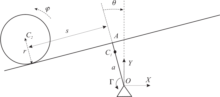
Figure 1: Diagram of the straight beam-and-ball system.

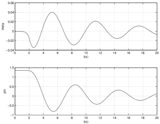
Figure 2: Stabilization of the Straight beam-and-ball system, $\theta\rightarrow 0$ and $\varphi\rightarrow 0$ (in radians).

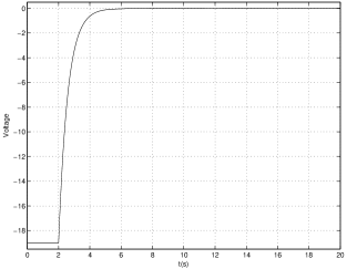
Figure 3: Voltage $u(t)$, supplied to the motor for the stabilization of the Straight beam-and-ball system.

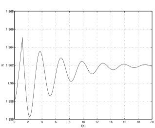
Figure 4: The reaction force $F(t)$, applied to the ball during the stabilization process.

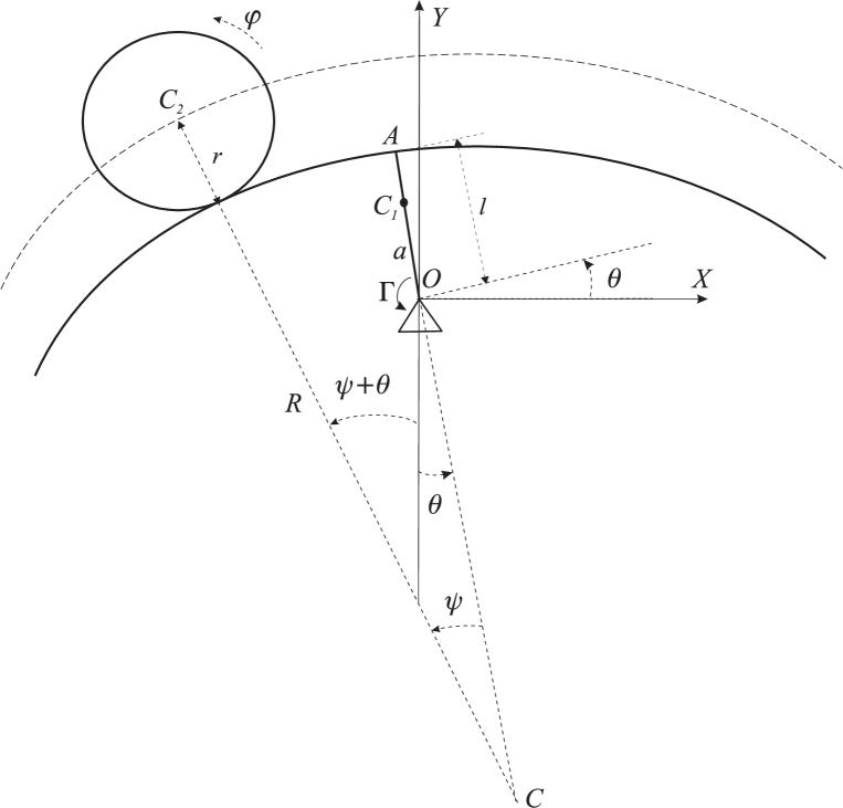
Figure 5: Diagram of the circular beam-and-ball system.

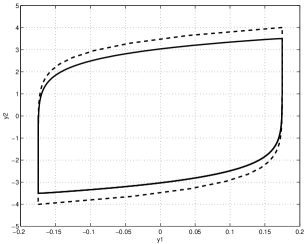
Figure 6: Controllability domain $Q$ (dashed line) for system (38) and basin of attraction $B$ (solid line) with $\gamma=4000$

.

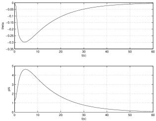
Figure 7: Stabilization of the Circular beam-and-ball system, $\theta\rightarrow 0$ and $\varphi\rightarrow 0$ (in radians).

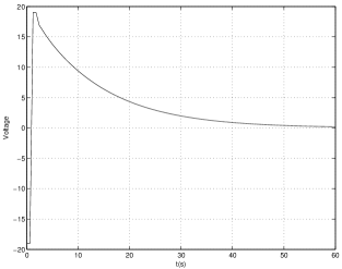
Figure 8: Voltage $u(t)$, supplied to the motor for the stabilization of the Circular beam-and-ball system.

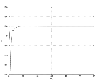
Figure 9: The reaction force $F(t)$, applied to the ball during the stabilization process.

References

- (1) J. Hauser, S. Sastry, and G. Meyer, “Nonlinear control design for slightly nonminimum phase systems. Application to V/STOL aircraft,” Automatica, vol. 28, no. 4, pp. 665–679, 1992.
- (2) M. Alimir and F. Boyer, “Fast generation of attractive trajectories for an under-actuated satellite. Application to feedback control design,” Journal of Optimization and Engineering, vol. 4, pp. 225–244, 2003.
- (3) W. J. Book and M. Majette, “Controller design for flexible, distributed parameter mechanical arms via combined state space and frequency domain techniques,” Transaction of ASME, Journal Dynamic Systems, Measurement and Control, vol. 105, pp. 245–254, 1983.
- (4) A. De Luca and B. Siciliano, “Closed-form dynamic model of planar multi-link lightweight robots,” IEEE Transaction System Man Cybernetics, vol. 21, no. 4, pp. 826–839, 1991.
- (5) K. J. Astrom and K. Furuta, “Swinging up a pendulum by energy control,” Automatica, vol. 36, no. 2, pp. 287–295, 2000.
- (6) A. A. Grishin, A. V. Lenskii, D. E. Okhotsimsky, D. A. Panin, and A. M. Formal’sky, “A control synthesis for an unstable object. An inverted pendulum,” Journal of Computer and System Sciences International, vol. 41, no. 5, pp. 685–694, 2002.
- (7) M. W. Spong, “The swing up control problem for the acrobot,” IEEE Control System Magazine, vol. 14, no. 1, pp. 49–55, 1995.
- (8) J. W. Grizzle, C. M. Moog, and C. Chevallereau, “Nonlinear control of mechanical systems with an unactuated cyclic variable,” IEEE Transactions on Automatic Control, vol. 50, no. 5, pp. 559–576, 2005.
- (9) Y. Aoustin and A. M. Formal’sky, “Design of reference trajectory to stabilize desired nominal cyclic gait of a biped,” in Proceedings International Workshop on Robot Motion and Control, ROMOCO’99, 1999, pp. 159–165.
- (10) ——, “Control design for a biped reference trajectory based on driven angles as functions of the undriven angle,” Journal of Computer and System Sciences International, vol. 42, no. 4, pp. 159–176, 2003.
- (11) F. Plestan, J. W. Grizzle, W. Westervelt, and G. Abba, “Stable walking of a 7-dof biped robot,” IEEE Transactions on Robotics and Automation, vol. 19, pp. 653–668, 2003.
- (12) J. Acosta, R. Ortega, and A. Astolfo, “Position feedback stabilization of mechanical systems with underactuation degree one,” in Proceedings of the 6th IFAC Symposium Nonlinear Control Systems, NOCOLS’04, 2004.
- (13) I. Fantoni and R. Lozano, Non linear control for underactuated mechanical systems. London: Springer-Verlag, Communications and control engineering series, 2002.
- (14) R. Olfati-Saber, “Nonlinear control of underactuated mechanical systems with application to robotics and aerospace vehicles,” Phd Thesis, Massachusetts Institute of Technology, 2001.
- (15) J. Hauser, S. Sastry, and P. Kokotović, “Nonlinear control via approximate input-output linearization,” IEEE Transactions. on Automatic Control, vol. 37, pp. 392–398, 1992.
- (16) A. R. Teel and L. Praly, “Tools for semiglbal stabilization by partial state and output feedback,” SIAM Journal of Control and Optimization, vol. 33, pp. 1443–1488, 1995.
- (17) A. R. Teel, “Using saturation to stabilize a class of single-input partially linear composite systems,” in IFAC NOLCOS’92 Symposium, May 1992, pp. 369–374.
- (18) R. Sepulchre, M. Janković, and P. Kokotović, Constructive Nonlinear Control. Springer-Verlag, 1997.
- (19) Y. Aoustin and A. M. Formal’sky, “On the stabilization of biped vertical posture in single support using internal torques,” Robotica, vol. 23, no. 1, pp. 65–74, 2005.
- (20) Y. Aoustin, A. M. Formal’sky, and Y. Martynenko, “Stabilisation of unstable equilibrium postures of a two-link pendulum using a flywheel,” Journal of Computer and System Sciences International, no. 2, pp. 16–23, 2006.
- (21) A. M. Formal’skii, Controllability and stability of systems with limited ressources. Nauka, Moscow, 1974, (In Russian).
- (22) T. Hu, Z. Lin, and L. Qiu, “Stabilization of exponentially unstable linear systems with saturating actuators,” IEEE Transactions on Automatic Control, vol. 46, no. 6, pp. 973–979, 2001.
- (23) D. M. Gorinevsky, A. M. Formal’sky, and A. Yu. Schneider, Force control of robotics systems. New-York: CRC Press, Boca Raton, 1997.
- (24) R. E. Kalman, P. L. Falb, and M. A. Arbib, Topics in mathematical system theory. McGrow-Hill Book Compagny, 1969.
- (25) G. A. Korn and T. M. Korn, Mathematical handbook for engineers and scientists. McGraw-Hill Book Company, 1968.
- (26) H. K. Khalil, Nonlinear system. New Jersey: Prentice Hall, 2002.
- (27) V. G. Boltyansky, Mathematical methods of optimal control. Nauka, Moscow, 1966, (In Russian).