Abstract

With present and upcoming SUSY searches both directly, indirectly and at accelerators, the need for accurate calculations is large. We will here go through some of the tools available both from a dark matter point of view and at accelerators. For natural reasons, we will focus on public tools, even though there are some rather sophisticated private tools as well.

The long awaited Large Hadron Collider (LHC) is expected to start taking data in 2009. The LHC research program has traditionally been centered around the discovery of the Higgs boson. However, the standard model description of this particle calls for New Physics. Until a few years ago, the epitome of this New Physics has been supersymmetry, which when endowed with a discrete symmetry called R-parity furnishes a good dark matter candidate. Recently a few alternatives have been put forward. Originally, they were confined to solving the Higgs problem, but it has been discovered that, generically, their most viable implementation (in accord with electroweak precision data, proton decay, etc.) fares far better if a discrete symmetry is embedded in the model. The discrete symmetry is behind the existence of a possible dark matter candidate.

From another viewpoint, stressed in many parts of this book, the last few years have witnessed spectacular advances in cosmology and astrophysics confirming that ordinary matter is a minute part of what constitutes the Universe at large. At the same time in which the LHC will be gathering data, a host of non collider astrophysical and cosmological observations with ever increasing accuracy will be carried out in search of dark matter. For example, the upcoming PLANCK experiment will make cosmology enter the era of precision measurements akin of what we witnessed with the LEP experiments.

The emergence of this new paradigm means it is of utmost importance to analyse and combine data from these upcoming observations with those at the LHC. This will also pave the way to search strategies for the next Linear Collider, LC. This important program is only possible if a cross-border particle-astroparticle collaboration is set up having at its disposal common or complementary tools to conduct global searches and analyses. Many groups, from erstwhile diverse communities, are now developing, improving, generalising, interfacing and exploiting such tools for the prediction and analysis of dark matter signals from a combination of terrestrial and non terrestrial observations, paying particular attention to the astrophysical uncertainties. Most of this work has been conducted in the context of supersymmetry, but the latest numerical tools are not limited to it.

In this chapter, we will go through some of the tools available both from a dark matter point of view and at accelerators. For natural reasons, we will focus on public tools, even though there are some rather sophisticated private tools as well. For supersymmetric dark matter calculations, one of the first public tools available was Neutdriver [1, 2]. It was a precursor in the field, but has by now been superceded by other more sophisticated tools. There are currently three publicly available codes for calculations of dark matter densities and dark matter signals: DarkSUSY [3, 4, 5], micrOMEGAs [6, 7, 8, 9] and IsaRED (part of ISASUSY/Isajet [10])

1 Annihilation cross section and the relic density

The general theory behind relic density calculations of dark matter particles is given in Chapter 7 [11]. Here we will focus on supersymmetric dark matter (neutralinos) and various tools available for calculating the relic density. There are currently three publicly available codes for calculating the relic density of neutralinos: DarkSUSY, micrOMEGAs and IsaRED. All three of these codes are capable of reading (and sometimes writing) SUSY Les Houches Accord (SLHA) files [13, 14] which allows for an easy interface between these codes and other tools to be described in Section 5.

We will in the following refer to these codes and how they calculate the relic density. We will use the notation of Chapter 7 [11] and only write down the equations needed to facilitate our discussions here.

1.1 The Boltzmann equation

In most supersymmetric models of interest for dark matter phenomenology, the lightest neutralino, $\chi$ is the lightest supersymmetric particle and our dark matter candidate. As such, we want to calculate the relic density of neutralinos in the Universe today as accurately as possible, which means that we need to solve the Boltzmann equation.

$$\frac{dn_{\chi}}{dt}=-3Hn_{\chi}-\langle\sigma_{\rm ann}v\rangle\left(n_{\chi}^{2}-n_{\chi,\,\rm eq}^{2}\right)$$ (1)

where $n_{\chi}$ is the number density of neutralinos, $H$ is the Hubble parameter, $\langle\sigma_{\rm ann}v\rangle$ is the thermally averaged annihilation cross section and $n_{\chi,\,\rm eq}$ is the equilibrium number density of neutralinos. This equation needs to be solved over time (or temperature) properly calculating the thermal average at each time step. When the neutralinos no longer can follow the chemical equilibrium density $n_{\chi,\,\rm eq}$, they are said to freeze-out. There are several complications in solving Eq. (1); for example, we may have resonances and thresholds in our annihilation cross section. The solution to this is to calculate the annihilation cross section in general relativistic form, for arbitrary relative velocities, $v$. Another complication is that other supersymmetric particles of similar mass will be present during freeze-out of the neutralinos. To solve this we need to take into account the so-called coannihilations between all the SUSY particles that are almost degenerate in mass with the neutralino (in practice, it is often enough to consider coannihilations between all SUSY particles up to about 50% heavier than the neutralino). Following the discussion in Chapter 7 [11], we can solve for the total number density of SUSY particles,

$$n=\sum_{i=1}^{N}n_{i}$$ (2)

instead of only the neutralino number density. It is also advantageous to rephrase the Boltzmann equation in terms of the abundance $Y=n/s$ and use $x=m_{\chi}/T$ as independent variable instead of time or temperature. When coannihilations are included, the Boltzmann equation (1) can then be written as

$$\frac{dY}{dx}=-\left(\frac{45}{\pi M_{P}^{2}}\right)^{-1/2}\frac{g_{*}^{1/2}m_{\chi}}{x^{2}}\left<\sigma_{\rm eff}v\right>(Y^{2}-Y_{eq}^{2})\,.$$ (3)

where $\langle\sigma_{\rm eff}v\rangle$ is given by [11, Eq. (7.18)]

1.2 Solving the Boltzmann equation

To solve the Boltzmann equation (3) we need to calculate the thermally averaged annihilation cross section $\langle\sigma_{\rm eff}v\rangle$ for each given time (temperature). This is typically quite CPU-intensive, and we therefore need to use some tricks. In DarkSUSY  [5], the solution is speeded up by tabulating $W_{\rm eff}$ in [11, Eq. (7.19)] , but using the momentum of the $\chi$, $p_{\rm eff}$ as independent variable instead of $s$. This tabulation takes extra care of thresholds and resonances making sure that they are tabulated properly. This tabulated $W_{\rm eff}$ is then used to calculate the thermal average $\langle\sigma_{\rm eff}v\rangle$ for each time (temperature), using [11, Eq. (7.18)] . The advantage with this method is that $W_{\rm eff}$ does not depend on temperature and instead the temperature dependence of $\langle\sigma_{\rm eff}v\rangle$ is completely taken care of by the other factors in [11, Eq. (7.18)]. Numerically, one needs to take special care of the modified Bessel functions $K_{1}$ and $K_{2}$ which both contain exponentials that need to be handled separately to avoid numerical underflows. The Boltzmann Equation (3) is then solved with a special implicit method with adaptive stepsize control, which is needed because the equation is stiff and develops numerical instabilities unless an implicit method is used. The details of the DarkSUSY method are as follows (see DarkSUSY manual [5]). The derivative $dY/dx$ in Eq. (3) is replaced with a finite difference $(Y_{n+1}\!-\!Y_{n})/h$, where $Y_{n}=Y(x_{n})$ and $x_{n+1}=x_{n}+h$. Then $Y_{n+1}$ is computed in two ways: first, the right hand side of Eq. (3) is approximated with $-\tfrac{1}{2}[\lambda_{n}(Y_{n}^{2}-Y_{eq,n}^{2})+\lambda_{n+1}(Y_{n+1}^{2}-Y_{eq,n+1}^{2})]$, where $\lambda(x)=\left(45/\pi M_{P}^{2}\right)^{-1/2}(g_{*}^{1/2}m/x^{2})\left<\sigma_{\rm eff}v\right>$, and an analytic solution is used for the resulting second-degree algebraic equation in $Y_{n+1}$; second, the right hand side of Eq. (3) is approximated with $-\lambda_{n+1}(Y_{n+1}^{2}-Y_{eq,n+1}^{2})$ and an analytic solution of the algebraic equation for $Y_{n+1}$ is used. The stepsize $h$ is reduced or increased to maintain the difference between the two approximate values of $Y_{n+1}$ within a specified error. Overall, the solution of the Boltzmann equation and the tabulation of $W_{\rm eff}$ solves for the relic density to within about 1%. If needed, higher accurary can also be chosen as an option.

In micrOMEGAs [7], $\langle\sigma_{\rm ann}v\rangle$ at a given temperature $T$ is arrived at by performing a direct integration and does not therefore rely on a tabulation of the matrix elements squared. Two modes are provided to perform the integration. In the accurate mode the program evaluates all integrals by means of an adaptive Simpson integration routine. It automatically detects all singularities of the integrands and checks the precision of the calculation increasing the number of points until an accuracy of $10^{-3}$ is reached. In the default mode (fast mode) the accuracy is not checked but a set of points is sampled according to the behaviour of the integrand: poles, thresholds and Boltzmann suppression at high momentum. The first integral over scattering angles is performed by means of a $5$-point Gauss formula. The accuracy of this mode is generally about $1\%$. The user can also test the precision of the approximation based on expanding the cross section in terms of its $s$ and $p$-wave components.

In the Boltzmann Equation, we need to know $g_{\rm eff}(T)$ and $h_{\rm eff}(T)$ that enter $g_{*}^{1/2}$ through [11, Eq. (7.9)]. In DarkSUSY, the default is to use the estimates in Ref. [15], but other options are also available. Typically, different estimates of $g_{\rm eff}(T)$ and $h_{\rm eff}(T)$ translate into relic densities different by a few percent.

IsaRED on the other hand does not solve the Boltzmann equation numerically, instead it finds the freeze-out temperature (the temperature when the annihilation rate equals the expansion rate of the Universe) and calculates the relic density from that (including remnant annihilations at later times). For the thermal averaged annihilation cross section, it uses the same relativistic treatment as DarkSUSY and micrOMEGAs.

1.3 Coannihilation criteria

Figure 1: Total differential annihilation rate per unit volume $dA/dp_{\rm eff}$ for the same model as in [11, Fig. 7.3], evaluated at a temperature $T=m_{\chi}/20$, typical of freeze-out. Notice the Boltzmann suppression at high $p_{\rm eff}$.

In principle, one should include all SUSY particle coannihilations when calculating the relic density. However, the heavier they are, the less abundant they will be and can thus be neglected. This is important to speed up the calculation, as we would otherwise spend most of our CPU cycles on calculating non-important coannihilation cross sections. One can estimate which particles to include, by investigating [11, Eq. (7.18)]. The modified Bessel function $K_{1}$ contains an exponential, the so called Boltzmann suppression, that will suppress all heavier particles. In Fig. 1, we show $dA/dp_{\rm eff}$ for the same model as in [11, Fig. 7.3]. $dA/dp_{\rm eff}$ is essentially (apart from normalization) the integrand in the numerator in [11, Eq. (7.18)]. Comparing the two figures, we clearly see the Boltzmann suppression of larger $p_{\rm eff}$, i.e. heavier coannihilating particles. We can quantify this by comparing the Boltzmann suppression factor for two coannihilating particles with masses $m_{i}$ and $m_{j}$ with the corresponding factor for the LSP, the $\chi$. The suppression factor for the coannihilating particles compared to the $\chi$ is roughly (neglecting the $p_{\rm eff}^{2}$ in [11, Eq. (7.18)]) given by

$$B=\frac{K_{1}((m_{i}+m_{j})/T)}{K_{1}(2m_{\chi}/T)}\simeq e^{-x\frac{m_{i}+m_{j}-2m_{\chi}}{m_{\chi}}}\quad;\quad x=\frac{m_{\chi}}{T}$$ (4)

At freeze-out we typically have $x\simeq 20$, which gives a suppression factor of $B\simeq 10^{-6}$ for coannihilation particles about 50% heavier than the LSP, $\chi$. In DarkSUSY, one can set the maximum mass fraction of coannihilation particles, $f=m_{i}/m_{\chi}$ that will be included in the calculation, whereas in micrOMEGAs one sets the minimum $B$ to allow instead. The defaults in DarkSUSY ($f=1.5$) and micrOMEGAs ($B_{\rm min}=10^{-6}$) are roughly equivalent. One should remember, though, that the value to choose depends on the particle physics model. For example, for chargino coannihilations, the $\chi^{+}\chi^{-}$ coannihilation cross section can be orders of magnitudes larger than the $\chi\chi$ annihilation cross sections and one should choose $f$ or $B_{\rm min}$ so that one does not accidentally neglect coannihilations that are important. For the MSSM, the default values of DarkSUSY and micrOMEGAs are typically sufficient for all interesting cases. IsaRED instead includes a preset collection of particles that are of relevance for the mSUGRA setup.

1.4 Annihilation cross section

At the heart of the relic density calculation are the annihilation and coannihilation cross sections. In the MSSM there are over 2800 sub-processes (not counting charged-conjugate final states) that can in principle contribute in the relic density calculation. It appears at first sight to be a daunting task to provide such a general code.

In DarkSUSY, all annihilation and coannihilation cross sections for the MSSM are calculated at tree level by hand with the help of symbolic programs like Reduce, Form or Mathematica. The calculations are performed with general expressions for the vertices in the Feynman rules and the results are converted to Fortran code. The vertices are then calculated numerically for any given MSSM model. The analytically calculated cross sections are differential in the angle of the outgoing particles, and the integration over the outgoing angle is performed numerically.

In micrOMEGAs, on the other hand, any annihilation and coannihilation cross sections are calculated automatically and generated on the fly. This is possible thanks to an interface to CalcHEP [16], which is an automatic matrix element/cross sections generator. This automation is carried one step further in that CalcHEP itself reads its MSSM model file (Feynman rules) from LanHEP [17], which outputs the complete set of Feynman rules from a simple coding of the Lagrangian, see section 5. In the first call to micrOMEGAs only those subprocesses needed for the given set of the MSSM parameters are generated. The corresponding “shared” library is stored on the user disk space and is accessible for all subsequent calls, thus each process is generated and compiled only once. This library is then filled with more and more processes whenever the user needs new processes for different MSSM scenarios. This avoids having to distribute a huge code with all the possible 2800 processes.

Both methods have advantages and disadvantages. In the DarkSUSY setup, no recalculation of the (analytical) annihilation cross sections is needed, which can speed things up. Also, the analytically calculated annihilation cross sections can be optimized to be faster. On the other hand, the micrOMEGAs setup makes it easier to adapt the code to non-MSSM cases. In both codes though, the actual Boltzmann equation solver is very general and works for any kind of WIMP dark matter, not only SUSY dark matter. In IsaRED, CompHEP [18] is used to calculate the annihilation and coannihilation cross sections for a subset of SUSY particles of relevance mostly for mSUGRA (the two lightest neutralinos, the lightest chargino, the left-handed eigenstates of sleptons and squarks, and gluinos). The expressions for the annihilation cross sections in IsaRED are not calculated on the fly, but are instead precalculated and included with the code.

2 Direct detection

Detailed expressions for detection rates in direct detection experiments are presented in Chapter 17 [19]. Here we focus on characteristics of the elastic scattering cross sections and event rates as they are implemented in numerical tools.

Direct detection rates depend on the differential elastic WIMP-nucleus cross section $d\sigma_{WN}/dE_{R}$, where $E_{R}$ is the energy of the recoiling nucleus:

$$\frac{d\sigma_{WN}}{dE_{R}}=\frac{m_{N}}{2\mu_{N}^{2}v^{2}}\Bigl{(}\sigma_{0}^{SI}F^{2}_{SI}(E_{R})+\sigma_{0}^{SD}F^{2}_{SD}(E_{R})\Bigr{)}.$$ (5)

Here $m_{N}$ is the nucleus mass, $\mu_{N}=m_{\chi}m_{N}/(m_{\chi}+m_{N})$ is the WIMP-nucleus reduced mass ($m_{\chi}$ being the WIMP mass), ${\bf v}$ is the WIMP-nucleus relative velocity before the collision, $\sigma_{0}^{SI,SD}$ are the spin-independent and spin-dependent cross sections at zero momentum transfer, and $F^{2}_{SI,SD}(E_{R})$ are the squares of the corresponding form factors (also called structure functions). In terms of these quantities, the directional and non-directional direct detection rates read

$$\frac{dR}{dE_{R}d\Omega_{q}} = \frac{\rho_{0}}{8\pi\mu_{N}^{2}m_{\chi}}\,\sigma_{WN}(E_{R})\,\hat{f}(v_{\rm min},\Omega_{q}),\qquad$$ (6)

$$\frac{dR}{dE_{R}} = \frac{\rho_{0}}{2\mu_{N}^{2}m_{\chi}}\,\sigma_{WN}(E_{R})\,\eta(v_{\rm min}),\qquad$$ (7)

where

$$\sigma_{WN}(E_{R}) = \sigma_{0}^{SI}F^{2}_{SI}(E_{R})+\sigma_{0}^{SD}F^{2}_{SD}(E_{R}),$$ (8)

$$\eta(v_{\rm min}) = \int_{v>v_{\rm min}}\frac{f({\bf v})}{v}\,d^{3}v,$$ (9)

$v_{\rm min}=[(m_{N}E_{R})/(2\mu_{N}^{2})]^{1/2}$ is the minimum WIMP speed which can cause a recoil of energy $E_{R}$, $\Omega_{q}$ is the direction of the nucleus recoil momentum of magnitude $q=\sqrt{2m_{N}E_{R}}$, and $\hat{f}(v_{\rm min},\Omega_{q})$ is the Radon transform of the velocity distribution function $f({\bf v})$.

An important property of Eqs. (6) and (7) is the factorization of the particle physics properties, $\sigma_{WN}(E_{R})$, and the astrophysics properties, $\rho_{0}\hat{f}(v_{\rm min},\Omega_{q})$ and $\rho_{0}\eta(v_{\rm min})$.

Dark matter codes such as DarkSUSY, IsaRED/RES and micrOMEGAs compute the particle physics and the astrophysics factors to various levels of precision and offer a number of choices for the form factors and the velocity distribution (more and more as they are upgraded). All codes provide the zero-momentum transfer cross sections (although some are still limited to the axial and scalar couplings of supersymmetric neutralinos), and most of the codes provide routines for direct detection rates off composite targets besides single nuclei.

For the spin-independent part, dark matter codes use the factorized form $\sigma_{WN}^{SI}(E_{R})=\sigma_{0}^{SI}F^{2}_{SI}(E_{R})$ with, in the notation of Chapter 17 [19],

$$\sigma_{0}^{SI}=\frac{4\mu_{n}^{2}}{\pi}\left[\Bigl{(}Zf^{p}+(A-Z)f^{n}\Bigr{)}^{2}+\frac{B_{N}^{2}}{256}\right].$$ (10)

Various expressions for the spin-independent form factor $F^{2}_{SI}(E_{R})$ are typically available. For example, DarkSUSY 5 automatically selects the best available form factor among Sums-of-Gaussians, Fourier-Bessel, and Helm parametrizations (see [20] for a comparison of these approximations).

The spin-dependent part is often not factorized, so as to use the same functions provided by detailed simulations at zero and non-zero momentum transfer. With the by-now-standard normalization of the spin structure functions in [21], one has

$$\sigma_{0}^{SD}F^{2}_{SD}(E_{R}) = \frac{32\mu_{N}^{2}G_{F}^{2}}{2J+1}\,\left[a_{0}^{2}S_{00}(E_{R})+a_{1}^{2}S_{11}(E_{R})+a_{0}a_{1}S_{01}(E_{R})\right]\qquad{~{}}$$ (11)

$$= \frac{32\mu_{N}^{2}G_{F}^{2}}{2J+1}\,\left[a_{p}^{2}S_{pp}(E_{R})+a_{n}^{2}S_{nn}(E_{R})+a_{p}a_{n}S_{pn}(E_{R})\right],\qquad{~{}}$$ (12)

where $a_{0}=a_{p}+a_{n}$, $a_{1}=a_{p}-a_{n}$,

$$S_{{pp}}(E_{R}) = S_{00}(E_{R})+S_{11}(E_{R})+S_{01}(E_{R})\,,$$ (13)

$$S_{{nn}}(E_{R}) = S_{00}(E_{R})+S_{11}(E_{R})-S_{01}(E_{R})\,,$$ (14)

$$S_{pn}(E_{R}) = 2\left[S_{00}(E_{R})-S_{11}(E_{R})\right]\,.$$ (15)

When the nuclear spin is approximated by the spin of the odd nucleon only, one finds [22]

$$S_{{pp}}(E_{R})=\frac{\lambda_{N}^{2}J(J+1)(2J+1)}{\pi},\quad S_{nn}(E_{R})=0,\quad S_{{pn}}(E_{R})=0,$$ (16)

for a proton-odd nucleus, and

$$S_{{pp}}(E_{R})=0,\quad S_{{nn}}(E_{R})=\frac{\lambda_{N}^{2}J(J+1)(2J+1)}{\pi},\quad S_{pn}(E_{R})=0,$$ (17)

for a neutron-odd nucleus. Here $\lambda_{N}$ is conventionally defined through the relation $\langle N|{\bf S}|N\rangle=\lambda_{N}\langle N|{\bf J}|N\rangle$, where $|N\rangle$ is the nuclear state, ${\bf S}$ is the nuclear spin, ${\bf J}$ is the nuclear total angular momentum. Tables of $\lambda_{N}^{2}J(J+1)$ values for several nuclei can be found in [23] and [24].

The quantities $f^{p}$, $f^{n}$, $B_{N}$, $a_{0}$, $a_{1}$ are sums of products of the WIMP-quark and WIMP-gluon coupling constants $\alpha_{q,G}^{S,V,A,P,T}$ (for scalar, vector, axial, pseudoscalar, and tensor currents) and of the contributions $f_{TG}$, $f_{Tq}$ and $\Delta_{q}$ of the gluons and each quark flavor to the mass and spin of protons and neutrons. Values for the nucleonic matrix elements of gluons and quarks, in practice values for $f_{TG}$, $f_{Tq}$ and $\Delta_{q}$, are either hardcoded or settable by the user. Values for the effective coupling constants $\alpha_{q}^{S,V,A,P,T}$ are either precomputed analytically (DarkSUSY) or computed numerically on the fly (micrOMEGAs). For example, the effective lagrangian at the zero momentum transfer for the interaction of a fermionic WIMP $\chi$ with quarks $q$ reads

$${\cal L}_{F} = \alpha_{q}^{S}\;\bar{\chi}\chi\;\bar{q}q+\alpha_{q}^{V}\;\bar{\chi}\gamma_{\mu}\chi\;\bar{q}\gamma^{\mu}q$$ (18)

$$+ \alpha_{q}^{P}\;\bar{\chi}\gamma_{5}\gamma_{\mu}\chi\;\bar{q}\gamma_{5}\gamma^{\mu}q+\tfrac{1}{2}\alpha_{q}^{T}\;\bar{\chi}\sigma_{\mu\nu}\chi\;\bar{q}\sigma^{\mu\nu}q.$$

In the case of a Majorana WIMP, like the neutralino in the MSSM, only operators even under $\chi\leftrightarrow\bar{\chi}$ are possible (i.e. $\alpha_{q}^{V}=\alpha_{q}^{T}=0$). In micrOMEGAs, the numerical values of the coefficients $\alpha_{q}$ are obtained combining appropriate matrix elements for $\chi q\to\chi q$ and $\bar{\chi}q\to\bar{\chi}q$ scattering at zero momentum transfer. For example,

$$\alpha_{q}^{S}+\alpha_{q}^{V}=-i\,\frac{\langle q(p_{1}),\chi(p_{2})|\hat{S}{\mathcal{O}_{S}}|q(p_{1}),\chi(p_{2})\rangle}{\langle q(p_{1}),\chi(p_{2})|{\mathcal{O}_{S}}{\mathcal{O}_{S}}|q(p_{1}),\chi(p_{2})\rangle}$$

$$\alpha_{q}^{S}-\alpha_{q}^{V}=-i\,\frac{\langle\bar{q}(p_{1}),\chi(p_{2})|\hat{S}{\mathcal{O}_{S}}|\bar{q}(p_{1}),\chi(p_{2})\rangle}{\langle\bar{q}(p_{1}),\chi(p_{2})|{\mathcal{O}_{S}}{\mathcal{O}_{S}}|\bar{q}(p_{1}),\chi(p_{2})\rangle}$$ (19)

where $\mathcal{O}_{S}=\bar{\chi}\chi\,\bar{q}q$, the $S$-matrix $\hat{S}=1-i{\cal L}$ is obtained from the complete Lagrangian at the quark level, and the scattering matrix elements on the right hand sides are computed with CalcHEP. More general cases, including a generic local WIMP-quark operators and WIMPs with spin-$0$ and spin-$1$, are presented in [9].

Loop contributions are essential in the treatment of the WIMP-quark and especially WIMP-gluon coupling constants. For example, for neutral WIMPs like the supersymmetric neutralino, there is no neutralino-gluon coupling at the tree-level and the gluon contribution to $\alpha^{S}$ arises at the one-loop level. Complete analytic one-loop calculations for neutralino-quark and neutralino-gluon couplings were performed in [25, 26]; these formulas are incorporated in DarkSUSY. Automatic numerical calculations of all $\alpha_{q}^{S,V,A,P,T}$ at one-loop from user-specified generic lagrangians (with approximate treatment of some of the loop corrections, see [9]) are currently available in micrOMEGAs.

3 Indirect detection

Indirect detection methods are many and varied. Here we focus on the following traditional methods: neutrinos from the Sun and the Earth, and gamma-rays, neutrinos, and charged cosmic rays (positrons, antiprotons and antideuterons) from annihilations in the galactic halo. There are also other indirect signals, like synchrotron emission, signals from cosmological halos (giving a diffuse flux), and indirect consequences of the presence of dark matter in stars, Chapter 29 [27], but we will not focus on them here. Most of the theory needed for this discussion is found in Chapters 24 [28], 25 [29] and 26 [30]; we use the notation in those chapters and elaborate on the formulae given there when needed.

The main public tools available to calculate indirect rates are DarkSUSY [3, 4, 5] and micrOMEGAs [6, 7, 8, 9]. In addition, there are also approximate simple formulae and parameterizations available that can be used, but we will here focus on the numerical codes.

3.1 Neutrinos from the Sun/Earth

To calculate the neutrinos from the Sun/Earth, we need to calculate the capture rate of neutralinos in the Sun/Earth, we then need to solve the evolution equation for capture and annihilation in the Sun/Earth, let the neutralinos annihilate in the centre of the Sun/Earth to produce neutrinos and finally let the neutrinos propagate to the neutrino detector at Earth (taking interactions and oscillations into account).

In Chapter 25 [29], approximate formulae are given for the capture rate in the Sun. These formulae are good for quick calculations, but they include several approximations; with numerical codes, we can actually do better. DarkSUSY is currently the only public code that includes neutrino fluxes from the Sun/Earth and uses the full expressions in Ref. [31], where the capture is integrated over the full Sun/Earth including capture on the 16 main elements for the Sun (and 11 for the Earth). In DarkSUSY, an arbitrary velocity distribution can be used if desired in place of the commonly assumed Maxwell-Boltzmann distribution. For example, the Earth does not capture WIMPs directly from the galactic halo, instead it captures from a distribution that has diffused into the solar system by gravitation interactions [32]. DarkSUSY uses a velocity distribution at the Earth based on numerical simulations that take this diffusion into account [33]. There are also indications from more recent numerical simulations of WIMP diffusion in the solar system [34] that heavier WIMPs will have a reduced capture rate in the Sun due to gravitational effects due to Jupiter. The DarkSUSY user can optionally include these effects.

After capture, the evolution equation for the number density accumulated in the Sun/Earth is solved to give the annihilation rate today. Once the WIMPs have accumulated in the centre of the Sun/Earth, they annihilate and eventually produce neutrinos. In DarkSUSY, the annihilation and propagation of neutrinos is handled by a separate code, WimpSim [35, 36]. WimpSim takes care of annihilations to standard model particles in the central regions of the Sun/Earth with the help of Pythia [37]. Energy losses and stopping of particles in the dense environments at the center of Sun/Earth are also included. All flavours of neutrinos (and antineutrinos) are then propagated out of the Sun/Earth, taking oscillations and interactions (the latter only relevant for the Sun) into account. This is done in a full three-neutrino-flavour setup [35]. Once at the detector, the neutrinos are let to interact and produce charged leptons and hadronic showers. WimpSim has been run for a range of annihilation channels and masses from 10 GeV to 10 TeV, and the results have been summarized as yield tables that are read and interpolated by DarkSUSY. These results agree very well with a similar analysis in Ref. [38], where parameterizations and downloadable data files are also given. For annihilation channels that are particle physics model dependent (like annihilation to Higgs bosons), the Higgs bosons are let to decay in flight in DarkSUSY and the resulting fluxes are calculated from their decay products (properly Lorentz boosted).

The routines in DarkSUSY are also general enough to be easily adapted to other particle dark matter candidates, like Kaluza Klein dark matter.

3.2 Charged cosmic rays

The theory behind propagation of charged cosmic rays in the galaxy is presented in Chapter 26 [30]. We will use the notation in that chapter. In principle, what we have to do is to solve the master equation [30, Eq. (26.4)] with appropriate diffusion coefficients, energy loss terms, source terms and boundary conditions. Currently, micrOMEGAs includes the source spectra for arbitrary SUSY models, but does not include the spectra after propagation. This will be included in future versions though, using the results in Ref. [39]. In DarkSUSY, both the source spectra and the spectra after propagation in various propagation models are included. DarkSUSY implements axisymmetric propagation models and spherically symmetric (or at least axisymmetric) halo models. In DarkSUSY, diffusion is assumed to take place only in space (i.e. the term $K_{EE}$ in [30, Eq. (26.4)]) is assumed to be negligible). However, it also offers a full interface and integration with the leading cosmic ray propagation code GALPROP [40] where more sophisticated propagation models can be used. For the halo density, several preset profiles are available, the default being an NFW profile [41]. However, the user can supply her/his own halo profile; if it is given in the form of [30, Eq. (26.15)] it is particularly simple to do so. For solar modulation, DarkSUSY offers a standard spherical force-field approximation as explained in Chapter 26 [30].

For the source spectra (i.e. the spectra before propagation), DarkSUSY uses a similar setup as for the neutrino fluxes from the Sun/Earth given above. A large set of annihilation channels are simulated with Pythia [37] in vacuum, for a range of masses, and the yields of antiprotons, positrons, gamma-rays and neutrinos are stored as data tables. These tables are then read and interpolated by DarkSUSY at run-time. Higgs boson decays are included stepping down the decay chain. micrOMEGAs currently uses the same data files as DarkSUSY, but both codes are planning on using new updated simulations in future releases.

For more details about the DarkSUSY implementation of antiproton fluxes, see Ref. [42]; for the positron fluxes, see Ref. [43]. The antideuteron fluxes are calculated from the antiproton fluxes with the method given in Ref. [44].

3.3 Gamma-rays and neutrinos

Gamma-ray and neutrino spectra from annihilation in the galactic halo can be calculated with both DarkSUSY and micrOMEGAs. As mentioned above, the DarkSUSY spectra are based upon Pythia simulations, which are then read in and interpolated by DarkSUSY. Currently, micrOMEGAs uses the same tables as DarkSUSY. DarkSUSY also includes internal bremsstrahlung photons [45] that can be very important in some parts of the parameter space (e.g. in the stau coannihilation region). DarkSUSY also includes the monochromatic gamma-ray lines from annihilation to $\gamma\gamma$ [46] and $Z\gamma$ [47] that occur at loop-level. Currently, the DarkSUSY (and consequently then also the micrOMEGAs) neutrino spectra from halo annihilations do not include neutrino oscillations, but this will be addressed in future versions.

Gamma-rays and neutrinos are not affected by propagation, and hence the flux can be written as

$$\frac{d^{2}\Phi_{\gamma/\nu}(\psi)}{dEd\Omega} \simeq 9.395\cdot 10^{-12}\left(\frac{dN_{\gamma/\nu}}{dE}\right)\left(\frac{\sigma v}{10^{-29}\ {\rm cm}^{3}{\rm s}^{-1}}\right)\left(\frac{10\,\rm{GeV}}{m_{\chi}}\right)^{2}$$ (20)

$$\times J\left(\psi\right)\;\rm{cm}^{-2}\;\rm{s}^{-1}\;\rm{sr}^{-1}\;,$$

where we have defined the dimensionless function

$$J\left(\psi\right)=\frac{1}{8.5\,\rm{kpc}}\cdot\left(\frac{1}{0.3\,{\rm GeV}/{\rm cm}^{3}}\right)^{2}\int_{\rm line\;of\;sight}\rho_{\chi}^{2}(l)\;d\,l(\psi)\;$$ (21)

with $\psi$ being the angle from the galactic centre direction to the direction of observation, and $dN_{\gamma/\nu}/dE$ being the spectrum of gamma-rays or neutrinos. The line of sight integral, Eq. (21), can be calculated for any spherically symmetric profile in DarkSUSY (whereas micrOMEGAs currently implements an isothermal profile only).

4 Exploring the parameter space

One problem that arises when exploring a specific supersymmetric model setup (e.g. mSUGRA or a low-energy MSSM model) is how to scan the parameter space. The dimensions of this parameter space, i.e. the number of free independent parameters, can be large. For example, the general MSSM model has 124 parameters (MSSM-124), 18 of which define the Standard Model (SM). If one assumes CP-conservation, the number of parameters reduces to 63 (MSSM-63), which is still a large number. Typically, one reduces the number of parameters still further with inspired theoretical insights (see Chapter 8 [48]). In Minimal Supergravity, for example, unification of coupling constants, of gaugino masses, and of scalar masses leaves only 23 parameters, i.e. SM+5, one of which is just a positive or negative sign. An intermediate model often used in neutralino dark matter studies (MSSM-25) has 25 parameters, i.e. SM+7.

One typically wants to find parameter values that are theoretically consistent, have a preferred relic density and are not already excluded by other searches (e.g. rare decays or other accelerator searches). The brute force method would be to scan over the parameter space with some kind of grid scan. One soon realizes that one can typically get a better efficiency in the scans (i.e. more points that pass the cuts, or a better sampling of different interesting regions in the parameter space) by scanning in the logarithm of the mass parameters instead of the mass parameters directly. For higher-dimensional parameter spaces, it is often also more advantageous to scan randomly instead of on a fixed grid.

However, none of these methods are very effective in finding regions of parameter space that pass all the cuts. The relic density cut alone discards many models because of the high precision with which we know the relic density of dark matter today. Hence, more sophisticated methods have evolved that are efficient in generating points inside the interesting regions. Most of these use a Markov Chain Monte Carlo (MCMC) [49, 50, 51, 52, 53, 54] to generate points according to a goal distribution specified by the researcher. The goal distribution can be a function without direct physical meaning (e.g. a Gaussian distribution that peaks in the desired region) or could have a statistical meaning (e.g. a likelihood function or a prior distribution in a Bayesian analysis). A recent public code to perform these tasks, and that is linked to DarkSUSY, micrOMEGAs and other codes, is SuperBayeS [53]. These advanced methods can be very effective in finding the interesting regions of the parameters space. However, when interpreting the distribution of points these methods produce, one should be very careful. The definition of “interesting” is different for different investigators, and the way points are generated always involves a prior in parameter space (even grid methods can be said to have a prior, namely a series of Dirac delta functions at each grid point). One could go to the extreme of producing any kind of results by choosing appropriate priors. Fig. 2, for example, shows the correlation between the direct detection rate and the relic density jokingly obtained with priors that reflect the anthropic principle.

Figure 2: A humorous scatter plot showing correlations that may arise with appropriate choices of priors while scanning parameter space: in this case, the priors reflect the anthropic principle.

When parameter space scans with priors are used to compute statistical inferences on data, e.g. likelihood contours [55], one should keep in mind their rather severe dependence on the priors, especially the priors on very poorly known parameters for which there are little or no experimental data (supersymmetric masses, e.g.). This dependence arises from the use of Bayes theorem, which gives the probability of the model parameter given the data (the likelihood) in terms of the probability of the data given the model parameters (the assumed distribution of experimental and theoretical errors) as

$${\rm Prob(model|data)}={\rm Prob(data|model)}\;\frac{{\rm Prob(model)}}{{\rm Prob(data)}}.$$ (22)

While the probability of the data Prob(data) is just a normalization constant, the probability of the model parameters Prob(model) is the prior representing the degree of belief or the relative preference the researcher has in specific values of the model parameters. When real experimental data on particle dark matter models are in, the dependence on the priors is expected to become less severe.

5 Interface with collider and precision measurements codes

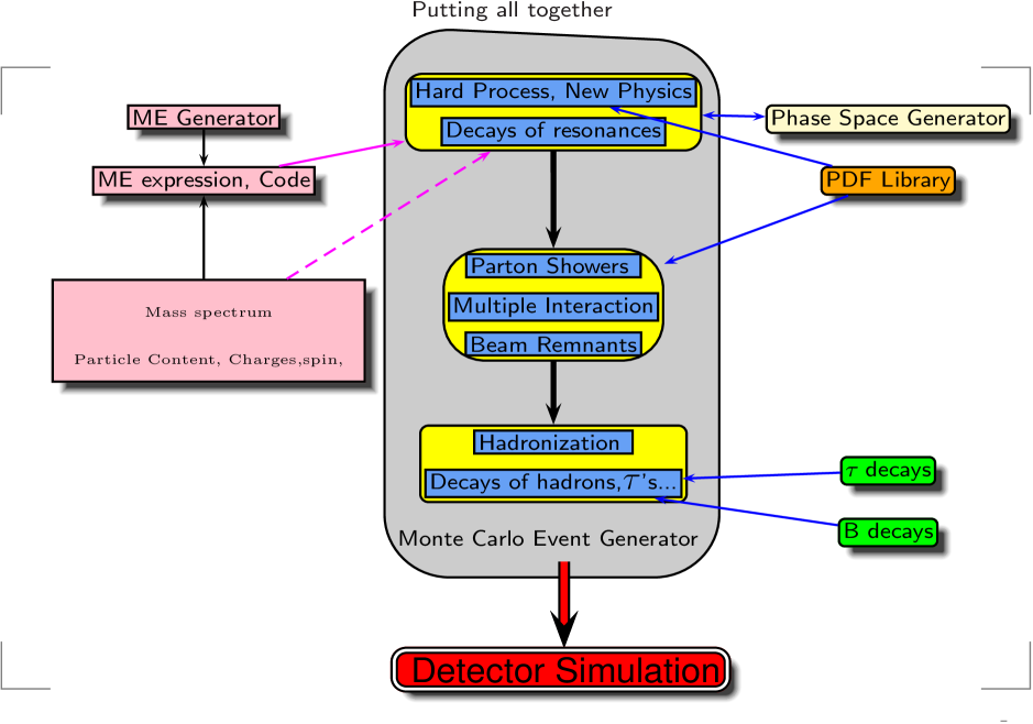
Figure 3: Modules that are involved in the construction of a Monte-Carlo event generator for particle collider physics.

Until a few years ago, one used constraints on the inferred amount of dark matter to delimit the parameter space of supersymmetry in order to narrow searches of supersymmetry at the colliders. Now with the improvement on the precision on the cosmological parameters one asks whether the LHC and LC can match the precision of the upcoming cosmology and astrophysics experiments in, for example, reconstructing the relic density once supersymmetry is identified [56, 54]. This may even bring a bonus in that one can test some cosmological and astrophysical assumptions, like indirectly “probing” the history of the early universe. For this programme to be feasible one needs to control the particle physics component with as much accuracy as possible. To be able to conduct a cohesive and self-consistent precision test of the origin of DM from the particle physics point of view one needs to calculate not only those dark matter cross sections but also the observables at the colliders that are predicted for the same dark matter model. Ideally, therefore, one would like a common tool that performs this task. In many instances this also requires that one goes beyond calculations at tree-level. This is especially true in the case of supersymmetry where it is known that radiative corrections can be large. Some progress in this direction has also been made recently within the SloopS Collaboration [57, 58, 59, 60, 61].

The dark matter codes for supersymmetry such as DarkSUSY, IsaRED/RES and micrOMEGAs include some higher order effects. Moreover, because of the complexity of the MSSM which has a large number of parameters and a large array of predictions, these codes also rely on other more specific codes that predict various other observables in supersymmetry. This concerns for example codes for the calculation of the spectrum based on the renormalisation group equations (RGE) that predict the low energy physical masses from an input at the unification scale in some constrained model of supersymmetry breaking. Spectrum calculators include Spheno [62], Softsusy [63], suspect [64] and ISASUGRA (part of ISAJET) [10]. These codes themselves may borrow from more specialised codes like those for the calculation of the Higgs masses, such as Feynhiggs [65]. The codes for the mass spectra may also feed in stand-alone codes for the calculation of precision measurements, like the calculation of $(g-2)_{\mu}$ and $B$ observables. Example of such codes or “flavour calculators” are (SUSYbsg [66], superiso [67]).

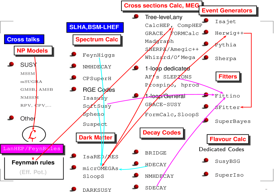
Figure 4: A collection of codes for the calculation of observables for supersymmetric particles. The event generators and the tree-level matrix elements codes cover also the Standard Model and in some instances other models of New Physics. The arrows show how the output of one code is fed into another code, which can itself be a source for other codes.

To make contact with LHC and LC observables one of course needs matrix elements for cross sections and decays of the supersymmetric particles. Many multipurpose matrix element generators exist for supersymmetry. Among them, Amegic [68], CalcHEP [16], CompHEP [18], Grace-SUSY [69], Omega [70], Madgraph [71]. Multipurpose matrix element generators can return results for any cross section or decay of a supersymmetric particle at the tree level. More dedicated and specialised codes in this category (cross sections and decays) usually improve by going beyond tree-level, among them PROSPINO [72] for the production of superparticles at a hadronic collider, HDECAY [73] for the decay of the Higgs and SDECAY [74] for the decay of other sparticles. Automatic codes for generic one-loop cross sections and decays with supersymmetry have also been completed recently as concerns the electroweak corrections and some classes of QCD corrections: Grace-susy-1loop [75] and SloopS [59, 60].

For simulations at the colliders one still needs to incorporate the matrix elements for the production (the hard process) and the decays (of the unstable superparticle resonances) into fully fledged Monte-Carlo generators. The latter include (i) parton shower (radiation), (ii) multiple interaction and beam remnant in hadronic machines and (iii) hadronisation. The main Monte-Carlo event generators are currently Herwig++ [76], ISAJET [10], Pythia [37] and SHERPA [77]. Fig. 3 shows the ingredients that go into a Monte-Carlo event generator. The mass spectrum module is what defines the model here, its content is therefore also encoded in the dark matter codes. One can use these generators to simulate the signatures of a particular model at the colliders and combine these findings with the manifestation of the same model in dark matter searches (direct and/or indirect), the prediction of the relic density in a particular cosmological model. One can constrain or reconstruct the model even further by taking into account observables from indirect precision measurements encoded in the flavour calculators. Codes (“Fitters”) that perform these fits or constraints have been written specifically with supersymmetry in mind; we can mention Fittino [78], SFitter [79] and SuperBayeS [53].

As we have seen, there is a very large variety of codes that cover different aspects of the phenomenology of supersymmetry. A recent compendium of these codes can be found in [80]. Because of the large number of parameters in a general supersymmetric model and because many modules are fed into other modules, it is best to avoid errors as much as possible when passing parameters from one code to another. Some of these errors can be as trivial as a problem of sign convention. The SUSY Les Houches Accord (SLHA) [13] allows an easy parsing for the MSSM parameters. This accord has been extended  [14] to deal with more general supersymmetric models, like the NMSSM for which a version of micrOMEGAs exists that uses or can be used with the NMHDECAY code [81], or with the inclusion of CP violation via CPSuperH [82].

Fig. 4 shows how the different codes for the calculation of supersymmetric observables both at the colliders and in dark matter searches or the evaluation of the relic density are interrelated. The calculation of the matrix elements needed for these codes requires first of all reading the Feynman rules. This in itself is a titanic endeavour because of the complexity of the MSSM and its extensions. For the dark matter codes, where a very large number of processes are involved, especially in the calculation of the relic density, practically the whole set of rules is called for. This is even more so for one-loop calculations. Special tools now exist to achieve this task whereby the model file (containing the Feynman rules) is generated automatically from just coding the Lagrangian in a manner as close to the calculation by hand. This was first done more than 10 years ago by LanHEP [17] based on $C$ for easy interface with CompHEP. The implementation here is very similar to the canonical coordinate representation. Use of multiplets and the superpotential is built-in to minimize human error. The ghost Lagrangian is derived directly from the BRST transformations. Very recently FeynRules [83] based on Mathematica enables to perform the same task and can output to different matrix element generators. MicrOMEGAs rapid development was in large part made possible because of the extensive automation based on LanHEP and CalcHEP/CompHEP. LanHEP has also been greatly extended to automatically implement a model file for calculations at one-loop. It is now possible to shift fields and parameters and thus generate counterterms most efficiently. LanHEP has been successfully interfaced with the highly efficient and automatised one-loop packages based on Feynarts/FeynCalc/LoopTools [84, 85, 86, 87]. The SloopS package is the combination of LanHEP and FeynArts, after a fully consistent and complete renormalisation of the MSSM has been completed [57, 58, 59, 60]. SloopS has been developed from the outset such that it is applicable to both high energy collider observables and for processes occurring at very low velocity such as is the case with dark matter particles. This will bring the cross breeding between dark matter and the collider predictions to a new level of precision, at least as far as the particle physics component is concerned.

Combining codes to be able to conduct global analyses for dark matter searches and the determination of its microscopic properties are witnessing an intense activity. If future colliders discover SUSY particles and probe their properties, one could predict the dark matter density and would constrain cosmology with the help of precision data provided by WMAP and PLANCK. It would be highly exciting if the precision reconstruction of the relic density from observables at the colliders does not match PLANCK’s determination. This would mean that the post-inflation era is most probably not radiation dominated (see Chapter 7 [11] for a discussion of alternative cosmologies before Big Bang nucleosynthesis and their effect on particle dark matter). The same collider data on the microscopic properties of DM, when put against a combination of data from direct/indirect detection, can also give strong constraints on the astrophysical properties of DM such as its distribution and clustering. These properties reveal much about galaxy formation [56, 54]. For this program to be carried through successfully, tools developed in the cosmology/astrophysics community and tools developed within the particle physics collider community (and their interfaces) are essential.

References

- [1] Gerard Jungman, Marc Kamionkowski, and Kim Griest. Supersymmetric dark matter. Phys. Rept., 267:195–373, 1996, hep-ph/9506380.
- [2] Gerard Jungman et al. Neutdriver. 2000. http://t8web.lanl.gov/people/jungman/neut-package.html.
- [3] Paolo Gondolo, Joakim Edsjo, Lars Bergstrom, Piero Ullio, and Edward A. Baltz. DarkSUSY: A numerical package for dark matter calculations in the MSSM. 2000, astro-ph/0012234.
- [4] Paolo Gondolo et al. DarkSUSY: A numerical package for supersymmetric dark matter calculations. 2002, astro-ph/0211238.
- [5] P. Gondolo et al. DarkSUSY: Computing supersymmetric dark matter properties numerically. JCAP, 0407:008, 2004, astro-ph/0406204.
- [6] G. Belanger, F. Boudjema, A. Pukhov, and A. Semenov. micrOMEGAs: A program for calculating the relic density in the MSSM. Comput. Phys. Commun., 149:103–120, 2002, hep-ph/0112278.
- [7] G. Belanger, F. Boudjema, A. Pukhov, and A. Semenov. micrOMEGAs2.0: A program to calculate the relic density of dark matter in a generic model. Comput. Phys. Commun., 176:367–382, 2007, hep-ph/0607059.
- [8] G. Belanger, F. Boudjema, A. Pukhov, and A. Semenov. micrOMEGAs: Version 1.3. Comput. Phys. Commun., 174:577–604, 2006, hep-ph/0405253.
- [9] G. Belanger, F. Boudjema, A. Pukhov, and A. Semenov. Dark matter direct detection rate in a generic model with micrOMEGAs2.1. 2008, arXiv:0803.2360 [hep-ph].
- [10] Frank E. Paige, Serban D. Protopopescu, Howard Baer, and Xerxes Tata. ISAJET 7.69: A Monte Carlo event generator for p p, anti-p p, and e+ e- reactions. 2003, hep-ph/0312045.
- [11] Graciela Gelmini and Paolo Gondolo. Dark Matter production mechanisms, in Particle Dark Matter, Editor: Gianfranco Bertone. Cambridge University Press, 2010.
- [12] A. Arbey and F. Mahmoudi. SuperIso Relic: A program for calculating relic density and flavor physics observables in Supersymmetry. 2009, arXiv:0906.0369 [hep-ph].
- [13] P. Skands et al. SUSY Les Houches accord: Interfacing SUSY spectrum calculators, decay packages, and event generators. JHEP, 07:036, 2004, hep-ph/0311123.
- [14] B. Allanach et al. SUSY Les Houches Accord 2. 2008, arXiv:0801.0045 [hep-ph].
- [15] Mark Hindmarsh and Owe Philipsen. WIMP dark matter and the QCD equation of state. Phys. Rev., D71:087302, 2005, hep-ph/0501232.
- [16] A. Pukhov. CalcHEP 3.2: MSSM, structure functions, event generation, batchs, and generation of matrix elements for other packages. 2004, hep-ph/0412191.
- [17] A. Semenov. LanHEP: A package for automatic generation of Feynman rules from the Lagrangian. Comput. Phys. Commun., 115:124–139, 1998.
- [18] E. Boos et al. CompHEP 4.4: Automatic computations from Lagrangians to events. Nucl. Instrum. Meth., A534:250–259, 2004, hep-ph/0403113.
- [19] David G. Cerdeño and Anne Green. Direct detection of WIMPs, in Particle Dark Matter, Editor: Gianfranco Bertone. Cambridge University Press, 2010, arXiv:1002.1912 [astro-ph].
- [20] Gintaras Duda, Ann Kemper, and Paolo Gondolo. Model independent form factors for spin independent neutralino nucleon scattering from elastic electron scattering data. JCAP, 0704:012, 2007, hep-ph/0608035.
- [21] J. Engel. Nuclear form-factors for the scattering of weakly interacting massive particles. Phys. Lett., B264:114–119, 1991.
- [22] Moqbil S. Alenazi and Paolo Gondolo. Directional recoil rates for WIMP direct detection. Phys. Rev., D77:043532, 2008, arXiv:0712.0053 [astro-ph].
- [23] John R. Ellis and Ricardo A. Flores. Elastic supersymmetric relic - nucleus scattering revisited. Phys. Lett., B263:259–266, 1991.
- [24] P. F. Smith and J. D. Lewin. Dark Matter Detection. Phys. Rept., 187:203, 1990.
- [25] Manuel Drees and Mihoko M. Nojiri. New contributions to coherent neutralino - nucleus scattering. Phys. Rev., D47:4226–4232, 1993, hep-ph/9210272.
- [26] Manuel Drees and Mihoko Nojiri. Neutralino-Nucleon Scattering Revisited. Phys. Rev., D48:3483–3501, 1993, hep-ph/9307208.
- [27] Gianfranco Bertone. Dark Matter and Stars, in Particle Dark Matter, Editor: Gianfranco Bertone. Cambridge University Press, 2010.
- [28] Lars Bergström and Gianfranco Bertone. Gamma rays, in Particle Dark Matter, Editor: Gianfranco Bertone. Cambridge University Press, 2010.
- [29] Francis Halzen and Dan Hooper. Neutrinos from WIMP annihilations in Sun and Earth, in Particle Dark Matter, Editor: Gianfranco Bertone. Cambridge University Press, 2010.
- [30] Pierre Salati, Fiorenza Donato, and Nicolao Fornengo. Indirect dark matter detection with cosmic antimatter, in Particle Dark Matter, Editor: Gianfranco Bertone. Cambridge University Press, 2010, arXiv:1003.4124 [astro-ph].
- [31] Andrew Gould. Resonant Enhancements in WIMP Capture by the Earth. Astrophys. J., 321:571, 1987.
- [32] A. Gould. Gravitational diffusion of solar system WIMPs. ”Astrop. J.”, 368:610–615, February 1991.
- [33] Johan Lundberg and Joakim Edsjo. WIMP diffusion in the solar system including solar depletion and its effect on earth capture rates. Phys. Rev., D69:123505, 2004, astro-ph/0401113.
- [34] Annika H. G. Peter and Scott Tremaine. Dynamics of WIMPs in the solar system and implications for detection. 2008, arXiv:0806.2133 [astro-ph].
- [35] Mattias Blennow, Joakim Edsjo, and Tommy Ohlsson. Neutrinos from WIMP Annihilations Using a Full Three- Flavor Monte Carlo. JCAP, 0801:021, 2008, arXiv:0709.3898 [hep-ph].
- [36] Joakim Edsjo. WimpSim - a general WIMP annihilation and neutrino propagation code for WIMP annihilations in the Sun/Earth. 2008. http://www.physto.se/~edsjo/wimpsim/.
- [37] Torbjorn Sjostrand, Stephen Mrenna, and Peter Skands. PYTHIA 6.4 physics and manual. JHEP, 05:026, 2006, hep-ph/0603175.
- [38] Marco Cirelli et al. Spectra of neutrinos from dark matter annihilations. Nucl. Phys., B727:99–138, 2005, hep-ph/0506298. http://www.marcocirelli.net/DMnu.html.
- [39] Pierre Brun. Towards a new tool for the indirect detection of dark matter: Building of a SuSy spectrum generator based on micrOMEGAs. 2006, astro-ph/0603387.
- [40] A. W. Strong and I. V. Moskalenko. Models for Galactic cosmic-ray propagation. Adv. Space Res., 27:717–726, 2001, astro-ph/0101068.
- [41] Julio F. Navarro, Carlos S. Frenk, and Simon D. M. White. The Structure of Cold Dark Matter Halos. Astrophys. J., 462:563–575, 1996, astro-ph/9508025.
- [42] Lars Bergstrom, Joakim Edsjo, and Piero Ullio. Cosmic antiprotons as a probe for supersymmetric dark matter? Astrophys. J., 526:215–235, 1999, astro-ph/9902012.
- [43] Edward A. Baltz and Joakim Edsjo. Positron Propagation and Fluxes from Neutralino Annihilation in the Halo. Phys. Rev., D59:023511, 1999, astro-ph/9808243.
- [44] Fiorenza Donato, Nicolao Fornengo, and Pierre Salati. Antideuterons as a signature of supersymmetric dark matter. Phys. Rev., D62:043003, 2000, hep-ph/9904481.
- [45] Torsten Bringmann, Lars Bergstrom, and Joakim Edsjo. New Gamma-Ray Contributions to Supersymmetric Dark Matter Annihilation. JHEP, 01:049, 2008, arXiv:0710.3169 [hep-ph].
- [46] Lars Bergstrom and Piero Ullio. Full one-loop calculation of neutralino annihilation into two photons. Nucl. Phys., B504:27–44, 1997, hep-ph/9706232.
- [47] Piero Ullio and Lars Bergstrom. Neutralino annihilation into a photon and a Z boson. Phys. Rev., D57:1962–1971, 1998, hep-ph/9707333.
- [48] John Ellis and Keith Olive. Supersymmetric Dark Matter Candidates, in Particle Dark Matter, Editor: Gianfranco Bertone. Cambridge University Press, 2010, arXiv:1001.3651 [astro-ph].
- [49] W.R. Gilks, S. Richardson, and eds. Spegelhalter, D.J. Markov chain monte carlo in practice. Chapman and Hall, 1996.
- [50] Joanna Dunkley, Martin Bucher, Pedro G. Ferreira, Kavilan Moodley, and Constantinos Skordis. Fast and reliable MCMC for cosmological parameter estimation. Mon. Not. Roy. Astron. Soc., 356:925–936, 2005, astro-ph/0405462.
- [51] Edward A. Baltz and Paolo Gondolo. Markov chain Monte Carlo exploration of minimal supergravity with implications for dark matter. JHEP, 10:052, 2004, hep-ph/0407039.
- [52] B. C. Allanach and C. G. Lester. Multi-Dimensional mSUGRA Likelihood Maps. Phys. Rev., D73:015013, 2006, hep-ph/0507283.
- [53] Roberto Ruiz de Austri, Roberto Trotta, and Leszek Roszkowski. A markov chain monte carlo analysis of the cmssm. JHEP, 05:002, 2006.
- [54] Edward A. Baltz, Marco Battaglia, Michael Edward Peskin, and Tommer Wizansky. Determination of dark matter properties at high-energy colliders. Phys. Rev., D74:103521, 2006, hep-ph/0602187.
- [55] Roberto Trotta, Farhan Feroz, Mike P. Hobson, Leszek Roszkowski, and Roberto Ruiz de Austri. The impact of priors and observables on parameter inferences in the Constrained MSSM. JHEP, 12:024, 2008, arXiv:0809.3792 [hep-ph].
- [56] B. C. Allanach, G. Belanger, F. Boudjema, and A. Pukhov. Requirements on collider data to match the precision of WMAP on supersymmetric dark matter. JHEP, 12:020, 2004, hep-ph/0410091.
- [57] F. Boudjema, A. Semenov, and D. Temes. Self-annihilation of the neutralino dark matter into two photons or a Z and a photon in the MSSM. Phys. Rev., D72:055024, 2005, hep-ph/0507127.
- [58] F. Boudjema, A. Semenov, and D. Temes. SUSY dark matter: Loops and precision from particle physics. Nucl. Phys. Proc. Suppl., 157:172–178, 2006.
- [59] N. Baro, F. Boudjema, and A. Semenov. Full one-loop corrections to the relic density in the MSSM: A few examples. Phys. Lett., B660:550–560, 2008, arXiv:0710.1821 [hep-ph].
- [60] N. Baro, F. Boudjema, and A. Semenov. Automatised full one-loop renormalisation of the MSSM I: The Higgs sector, the issue of tan(beta) and gauge invariance. 2008, arXiv:0807.4668 [hep-ph].
- [61] A. Freitas, A. von Manteuffel, and P. M. Zerwas. Slepton production at and linear colliders. (Addendum). Eur. Phys. J., C40:435–445, 2005, hep-ph/0408341.
- [62] Werner Porod. SPheno, a program for calculating supersymmetric spectra, SUSY particle decays and SUSY particle production at colliders. Comput. Phys. Commun., 153:275–315, 2003, hep-ph/0301101.
- [63] B. C. Allanach. SOFTSUSY: A C++ program for calculating supersymmetric spectra. Comput. Phys. Commun., 143:305–331, 2002, hep-ph/0104145.
- [64] Abdelhak Djouadi, Jean-Loic Kneur, and Gilbert Moultaka. SuSpect: A Fortran code for the supersymmetric and Higgs particle spectrum in the MSSM. Comput. Phys. Commun., 176:426–455, 2007, hep-ph/0211331.
- [65] S. Heinemeyer, W. Hollik, and G. Weiglein. FeynHiggs: a program for the calculation of the masses of the neutral CP-even Higgs bosons in the MSSM. Comput. Phys. Commun., 124:76–89, 2000, hep-ph/9812320.
- [66] G. Degrassi, P. Gambino, and P. Slavich. SusyBSG: a fortran code for BR[] in the MSSM with Minimal Flavor Violation. Comput. Phys. Commun., 179:759–771, 2008, arXiv:0712.3265 [hep-ph].
- [67] F. Mahmoudi. SuperIso: A program for calculating the isospin asymmetry of in the MSSM. Comput. Phys. Commun., 178:745–754, 2008, arXiv:0710.2067 [hep-ph].
- [68] F. Krauss, R. Kuhn, and G. Soff. AMEGIC++ 1.0: A matrix element generator in C++. JHEP, 02:044, 2002, hep-ph/0109036.
- [69] J. Fujimoto et al. GRACE/SUSY: Automatic generation of tree amplitudes in the minimal supersymmetric standard model. Comput. Phys. Commun., 153:106–134, 2003, hep-ph/0208036.
- [70] Wolfgang Kilian, Thorsten Ohl, and Jurgen Reuter. WHIZARD: Simulating Multi-Particle Processes at LHC and ILC. 2007, arXiv:0708.4233 [hep-ph].
- [71] Johan Alwall et al. MadGraph/MadEvent v4: The New Web Generation. JHEP, 09:028, 2007, arXiv:0706.2334 [hep-ph].
- [72] W. Beenakker, R. Hopker, and M. Spira. PROSPINO: A program for the PROduction of Supersymmetric Particles In Next-to-leading Order QCD. 1996, hep-ph/9611232.
- [73] A. Djouadi, J. Kalinowski, and M. Spira. HDECAY: A program for Higgs boson decays in the standard model and its supersymmetric extension. Comput. Phys. Commun., 108:56–74, 1998, hep-ph/9704448.
- [74] M. Muhlleitner, A. Djouadi, and Y. Mambrini. SDECAY: A Fortran code for the decays of the supersymmetric particles in the MSSM. Comput. Phys. Commun., 168:46–70, 2005, hep-ph/0311167.
- [75] Junpei Fujimoto et al. Two-body and three-body decays of charginos in one-loop order in the MSSM. Phys. Rev., D75:113002, 2007.
- [76] M. Bahr et al. Herwig++ Physics and Manual. Eur. Phys. J., C58:639–707, 2008, arXiv:0803.0883 [hep-ph].
- [77] T. Gleisberg et al. Event generation with SHERPA 1.1. 2008, arXiv:0811.4622 [hep-ph].
- [78] Philip Bechtle, Klaus Desch, and Peter Wienemann. Fittino, a program for determining MSSM parameters from collider observables using an iterative method. Comput. Phys. Commun., 174:47–70, 2006, hep-ph/0412012.
- [79] Remi Lafaye, Tilman Plehn, and Dirk Zerwas. SFITTER: SUSY parameter analysis at LHC and LC. 2004, hep-ph/0404282.
- [80] B. C. Allanach. SUSY Predictions and SUSY Tools at the LHC. 2008, arXiv:0805.2088 [hep-ph].
- [81] Ulrich Ellwanger, John F. Gunion, and Cyril Hugonie. NMHDECAY: A Fortran code for the Higgs masses, couplings and decay widths in the NMSSM. JHEP, 02:066, 2005, hep-ph/0406215.
- [82] J. S. Lee et al. CPsuperH: A computational tool for Higgs phenomenology in the minimal supersymmetric standard model with explicit CP violation. Comput. Phys. Commun., 156:283–317, 2004, hep-ph/0307377.
- [83] Neil D. Christensen and Claude Duhr. FeynRules - Feynman rules made easy. 2008, arXiv:0806.4194 [hep-ph].
- [84] T. Hahn and M. Perez-Victoria. Automatized one-loop calculations in four and D dimensions. Comput. Phys. Commun., 118:153–165, 1999, hep-ph/9807565.
- [85] Thomas Hahn. Generating Feynman diagrams and amplitudes with FeynArts 3. Comput. Phys. Commun., 140:418–431, 2001, hep-ph/0012260.
- [86] Thomas Hahn and Christian Schappacher. The implementation of the minimal supersymmetric standard model in FeynArts and FormCalc. Comput. Phys. Commun., 143:54–68, 2002, hep-ph/0105349.
- [87] Thomas Hahn. Automatic loop calculations with FeynArts, FormCalc, and LoopTools. Nucl. Phys. Proc. Suppl., 89:231–236, 2000, hep-ph/0005029.