Halo model description of the non-linear dark matter power spectrum at $k\gg 1$ Mpc^-1

Abstract

Accurate knowledge of the non-linear dark-matter power spectrum is important for understanding the large-scale structure of the Universe, the statistics of dark-matter haloes and their evolution, and cosmological gravitational lensing. We analytically model the dark-matter power spectrum and its cross-power spectrum with dark-matter haloes. Our model extends the halo-model formalism, including realistic substructure population within individual dark-matter haloes and the scatter of the concentration parameter at fixed halo mass. We consider three prescriptions for the mass-concentration relation and two for the substructure distribution in dark-matter haloes. We show that this extension of the halo model mainly increases the predicted power on the small scales, and is crucial for proper modeling the cosmological weak-lensing signal due to low-mass haloes. Our extended formalism shows how the halo model approach can be improved in accuracy as one increases the number of ingredients that are calibrated from $n$-body simulations.

1 Introduction

Accurate studies of large-scale cosmic structures and galaxy clustering became possible with the advent of large galaxy redshift surveys (Guzzo et al., 2000; Meneux et al., 2009). Different analyses have been carried out depending on galaxy luminosity, color and morphology (Norberg et al., 2002; Zehavi et al., 2005; Padmanabhan et al., 2007). According to the standard scenario of structure formation, galaxies with dissimilar features reside in different dark matter haloes and have experienced varied formation histories.

Galaxies are believed to form and reside in dark-matter haloes that extend much beyond their observable radii. Some of them are located at halo centers while others orbit around it, constituting the satellite population. Dark-matter haloes form by gravitational instability from dark-matter density fluctuations (Bond et al., 1991; Lacey & Cole, 1993) and subsequently merge to form increasingly large haloes as cosmic time proceeds. Gas follows the dark-matter density perturbations. Once it reaches sufficiently high densities, dissipative processes, shocks and cooling allow stars to form from this gas (White & Rees, 1978; Kauffmann et al., 1999). While the main lines of this scenario are widely accepted, its details are still poorly understood.

The clustering strength of a given galaxy population is related to that of the dark matter halos which host the galaxies. It is possible to provide an accurate description of clustering in the small-scale non-linear regime even if one has no knowledge of how the haloes themselves are clustered (Sheth & Jain, 1997; Smith et al., 2003). The halo-model of matter clustering (Scherrer & Bertschinger, 1991; Peacock & Smith, 2000; Seljak, 2000; Scoccimarro et al., 2001; Cooray & Sheth, 2002), which has been the subject of much recent interest, allows a parametrization of clustering even on large scales.

To date, almost all analytic work based on the halo-model approach assumes that haloes are spherically symmetric and that the matter density distribution around each halo centre is smooth. However, numerical simulations of hierarchical clustering have shown that haloes are neither spherically symmetric (Jing & Suto, 2002; Allgood et al., 2006; Hayashi et al., 2007) nor smooth (Moore et al., 1998; Springel et al., 2001; Gao et al., 2004; De Lucia et al., 2004; Tormen et al., 2004; Giocoli et al., 2008). About $10\%$ of the mass in cluster-sized haloes is associated with subclumps. A halo model which includes the effects of halo triaxiality on various clustering statistics is developed in Smith & Watts (2005); Smith et al. (2006), and formalism to include halo substructures was developed by Sheth & Jain (2003).

The main purpose of this work is to include recent advances in our understanding of halo substructures into the halo model approach. This is because an accurate model of substructures is a necessary first step to modeling the small scale weak gravitational lensing convergence and shear signals (Bartelmann & Schneider, 2001; Hagan et al., 2005) and for the substructure contribution to the gravitational flexion (Bacon et al., 2006).

The present paper is organized as follows. In Sect. 2, we describe the ingredients of our extension of the halo model: the properties of subhaloes and the substructure mass function. In Sect. 3, we show how to incorporate these into the halo model. Cross-correlations between haloes and mass as well as clumps and mass are studied in Sect. 4. Sect. 5 summarizes our methods and conclusions.

2 The model

We assume a flat $\mathrm{\Lambda}$CDM cosmological model consistent with a combined analysis of the 2dFGRS (Colless et al., 2001) and first-year WMAP data (Spergel et al., 2003). It has the parameters ($\Omega_{m}$, $\Omega_{b}$, $h$, $n$, $\sigma_{8}$)=(0.25, 0.045, 0.73, 1, 0.9). This is the model adopted by Springel et al. (2005) for the Millennium Simulation (hereafter MS), against which we test our model. Our linear power spectrum uses the transfer function by Eisenstein & Hu (1998), which takes baryonic acoustic oscillations into account, in agreement with CMBFAST (Seljak & Zaldarriaga, 1996) to $1\%$.

2.1 Halos

2.1.1 Mass function

For modeling the non-linear dark-matter power spectrum, we require the redshift evolution of the number density of collapsed haloes, $n(M,z)$. According to the spherical collapse model, a density fluctuation collapses when and where the linearly evolved density field smoothed with a top-hat filter exceeds the critical value $\delta_{c}(z)$ at that redshift. The distribution of collapsed peak heights is Gaussian when expressed in terms of the variable $\mu(M,z)=\delta_{c}(z)/\sqrt{S(M)}$, where $S(M)$ is the variance of a halo of mass $M$, if the collapse is not influenced by the surrounding gravitational field (Press & Schechter, 1974; Bond et al., 1991; Lacey & Cole, 1993). Following this idea, one can write the halo number density in the form

$$\nu f(\nu)=\dfrac{M^{2}}{\bar{\rho}}n(M,z)\dfrac{\mathrm{d}\log(M)}{\mathrm{d}\log(\nu)}\,,$$ (1)

where $\nu=\mu^{2}$ ($f(\mu)\mathrm{d}\mu$ is Gaussian for a fixed threshold $\delta_{c}$), and $\bar{\rho}$ is the mean matter density of the Universe.

However, the dark-matter halo mass functions measured in $N$-body simulations are far from Gaussian. The Press & Schechter (1974) formula over-predicts the abundance of low-mass haloes and under-predicts that of high-mass systems (Sheth & Tormen, 1999). This is because the collapse of the haloes is affected by the gravitational tidal field of the surrounding matter (Sheth et al., 2001). Different functional forms have been proposed to fit the simulation results (Sheth & Tormen, 1999; Jenkins et al., 2001). We use the Sheth & Tormen (1999) mass function because it is well tested against numerical simulations and easily parametrised in terms of the variable $\nu$ which we shall use throughout.

2.1.2 Bias

Since the halo model assumes that all matter in the universe is in collapsed systems, we need to model the ratio between the power spectra of dark-matter haloes and of the dark matter, i.e. the bias parameter, to compute the dark-matter power spectrum. To be consistent with our choice of the mass function, we also use the bias parameter $b(\nu)$ derived by Sheth & Tormen (1999). When expressed in terms of the peak height $\nu$, the bias parameter is independent of redshift. We recall that both the mass function and the bias parameter by Sheth & Tormen (1999) reproduce the original equations by Press & Schechter (1974) and Mo & White (1996) when specialized to isolated spherical collapse. At fixed redshift, the bias is an increasing function of the halo mass. More massive haloes (forming later and having a lower concentration) are more biased compared to less massive haloes (forming earlier and with a higher concentration). This has been confirmed by recent $N$-Body simulations.

Different improvements of the bias factor have been proposed (Jing, 1998; Governato et al., 1999; Sheth et al., 2001; Mandelbaum et al., 2005). Recent analyses have shown interesting features and unexpected results in view of the standard excursion-set formalism (Sheth & Tormen, 2004), also confirmed by Gao et al. (2005); Faltenbacher & White (2010). At masses exceeding $M_{*}$ (i.e. peak heights $\nu>1$), haloes in the same mass bin but with lower concentration (and thus lower formation redshift) are more biased than those with high concentrations, with a scatter of $\approx 20\%$ around the mean. The opposite holds for masses less than $M*$ ($\nu<1$). There is currently no accurate analytic model which allows a simple parametrization of the ‘assembly bias’ effect, so we have decided to continue using a bias parameter that depends on halo mass alone. Our algorithm can be easily extended by a new model for the bias factor if needed.

2.1.3 Density profiles

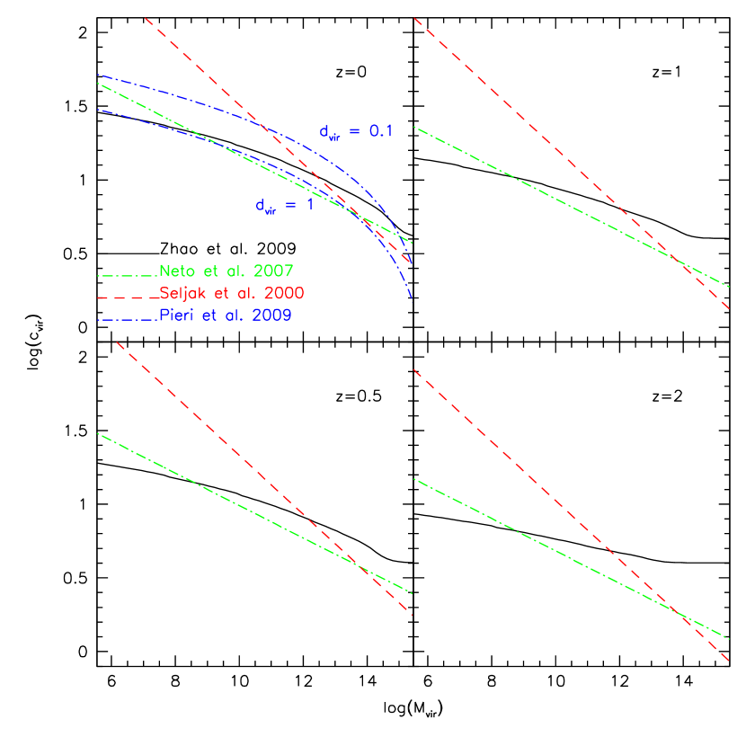
Figure 1: Mass-concentration relations of dark-matter haloes at four different redshifts. The solid, dash-dotted and dashed curves show the models by Zhao et al. (2009), Neto et al. (2007) and Seljak (2000) at redshifts $z$=0, 0.5, 1 and 2, respectively. In the top-left panel, we also show the mass-concentration relation for substructures estimated by Pieri et al. (2009) fitting the results of the Aquarius simulation for clumps located at the virial radius ($d_{vir}=1$) and at $0.1R_{vir}$ from the host-halo centre ($d_{vir}=0.1$). Notice that this fit has been rescaled to the definition of the virial radius adopted in this work.

Various different definitions for the virial overdensity $\Delta_{h}$ have been used in the literature. Some authors (Jenkins et al., 2001; Gao et al., 2004) use $\Delta_{200c}$, corresponding to $200$ times the critical density, or $\Delta_{200b}$, defined as $200$ times the background density (Diemand et al., 2007). Others (Sheth & Tormen, 1999; Sheth et al., 2001; Bullock et al., 2001; Jing & Suto, 2002) choose $\Delta_{h}=\Delta_{vir}$ according to the spherical collapse model (Peebles, 1980; Kitayama & Suto, 1996; Bryan & Norman, 1998). Here, we adopt $\Delta_{h}=\Delta_{vir}$ and use the virial overdensities given by Eke et al. (1996), which are related to the virial mass $M_{vir}$ by

$$M_{vir}=\frac{4\pi}{3}R_{vir}^{3}\frac{\Delta_{vir}}{\Omega_{m}(z)}\Omega_{0}\rho_{c}\,.$$ (2)

Cosmological $N$-body simulations (Navarro et al., 1996; Power et al., 2003; Neto et al., 2007; Gao et al., 2008) have shown that the dark-matter density in isolated haloes has a universal radial profile whose slope steepens from $-1$ near the centre to $-3$ towards the virial radius,

$$\rho(r|M_{vir})=\dfrac{\rho_{s}}{r/r_{s}\left(1+r/r_{s}\right)^{2}}\,,$$ (3)

where $r_{s}$ is the scale radius of the halo. Its concentration is defined as $c_{vir}=R_{vir}/r_{s}$. The amplitude $\rho_{s}$ sets the dark-matter density at the scale radius,

$$\rho_{s}=\dfrac{M_{vir}}{4\pi r_{s}^{3}}\left[\ln(1+c_{vir})-\dfrac{c_{vir}}{1+c_{vir}}\right]^{-1}\;.$$ (4)

Note that $c_{vir}$, and thus also $\rho_{s}$, depend on halo mass; we expand on this in the next subsection.

We shall need in the following an expression for the normalized Fourier transform of this density profile, truncated at the virial radius,

$$u(k|M)=\int_{0}^{R_{vir}}\frac{4\pi r^{2}}{M}\frac{\sin kr}{kr}\rho(r|M)\,\mathrm{d}r\;.$$ (5)

For the NFW profile, this integral has a convenient analytic expression (see Scoccimarro et al., 2001).

2.1.4 Mass-concentration relations

Motivated by numerical simulations and by previous halo-model studies, we consider three prescriptions for the mass-concentration relation to study uncertainties and differences in the recovery of the non-linear dark-matter power spectrum by means of the halo model (Seljak, 2000; Cooray & Sheth, 2002). These are:

1. C1 (Neto et al., 2007):

   $$c^{N}_{vir}(z)=\frac{c_{14}}{(1+z)}\left[\frac{M}{10^{14}}\right]^{-0.11}\;.$$ (6)

   This relation was obtained by Neto et al. (2007) by fitting the complete sample of haloes at $z=0$ in the Millennium Simulation (Springel et al., 2005). The value of the concentration of a $10^{14}M_{\odot}/h$ halo estimated by Neto et al. (2007) for an enclosed mean density of $200$ times the critical density has been rescaled to the virial overdensity. To rescale the normalization of the relation, we use the relation between $c_{200}$ and $c_{vir}$ presented in Macciò et al. (2008) at $z=0$.

2. C2 (Seljak, 2000):

   $$c^{S}_{vir}(z)=\frac{9}{(1+z)}\left[\frac{M}{M_{*0}}\right]^{-0.2}\;.$$ (7)

   This steeper model was used by Seljak (2000) in order to follow the Peacock & Dodds (1996) fit for the standard CDM model adopted. The mass $M_{*0}$ represents the typical collapsed mass at $z=0$ such that $\delta_{c}(0)=\sigma(M_{*0})$. Here, $\sigma(M)$ is the rms fluctuation in the linear density-fluctuation field when smoothed with a top-hat filter which contains mass $M$. In this case, we set the concentration of an $M_{*}$ halo to $9$ in order to reproduce the non-linear power-spectrum of the Millennium Simulation at $z=0$. Models C1 and C2 incorporate the redshift evolution of the mass-concentration relation proposed by Bullock et al. (2001).

3. C3 (Zhao et al., 2009):

   $$c^{Z}_{vir}(z)=4\left[1+\left(\frac{t(z)}{3.75\,t_{0.04}}\right)^{8.4}\right]^{1/8}\;.$$ (8)

   This model was proposed by Zhao et al. (2009) studying the mass-accretion history of dark-matter haloes in different cosmological models. They developed a model for the mass accretion history and related the concentration of an isolated halo to the time or redshift $z$ when it had assembled $4\%$ of its final mass. This is qualitatively motivated by the expectation that the structure of a halo should depend on its formation history. The correlation of the halo concentration with the time $t_{0.04}$ is purely empirical. For a detailed explanation of how to implement model C3, see Appendix A of Zhao et al. (2009). So far, the model lacks a detailed physical justification. However, it expresses the notion that dark-matter haloes form first as consequence of a violent relaxation process (White, 1996) which sets the value of the concentration near $4$. Subsequent accretion adds material primarily to the outer shells. A minimum value of $\sim 4$ means that the mass-concentration relation is expected to flatten at high redshifts, where haloes have had only had time to undergo the violent relaxation process.

   This flattening of the mass-concentration relation at high redshift was first discussed by Zhao et al. (2003b). Based on a combination of $N$-body simulations with different resolutions, they found that the mass dependence of halo concentrations weakens with increasing redshift. Later, Gao et al. (2008) and Duffy et al. (2008) confirmed these results studying haloes at different redshifts in the Millennium Simulation and with a different set of numerical simulations, respectively. They proposed different power-law fits at various redshifts, but these are less complete than model C3.

Figure 2: Left: Substructure mass function at the present time for different host-halo masses. Middle: Dependence of substructure mass fraction $f_{s}$ on host-halo mass. Curves show $f_{s}$ in subhalos above the minimum mass, as labeled. Right: Dependence of number of substructures on host halo mass, expressed in units of the number in an $M_{*}$-halo. The solid line has a slope of unity.

In Fig. 1, we show the mass-concentration relations described above at four different redshifts, $z=0$, $0.5$, $1$ and $2$. While models C1 and C2 preserve their slopes as the redshift increases, model C3 flattens towards higher redshift. Also, notice that in model C3, no haloes have a concentration $<4$, the value set by the violent relaxation process.

2.1.5 Concentration distributions

We shall adopt two ways of assigning concentrations to haloes of fixed mass, a deterministic model D1 and a stochastic model D2.

1. D1: In common applications of the halo model, any scatter in the concentration parameter at fixed halo mass is neglected. The conditional distribution $p(c|M)$ is thus assumed to be a delta distribution,

   $$p(c|M)=\delta\left[c-\bar{c}(M,z)\right]\;,$$ (9)

   where $\bar{c}(M,z)$ is given by any of the mass-concentration relations C1, C2 or C3, see Eqs. (6, 7, 8).

2. D2: However, numerical simulations have shown that at a fixed halo mass, different assembly histories yield different values of the concentration (Navarro et al., 1996; Jing, 2000; Wechsler et al., 2002). For example, Zhao et al. (2003a, b) proposed that the concentration could be related to the phase of fast accretion of the main halo progenitor. In general, haloes formed at higher redshift are more concentrated than haloes formed more recently. The distribution around the mean value $\bar{c}$ found in numerical simulations is well described by a log-normal form,

   $$p(c|M)=\frac{1}{\sqrt{2\pi\sigma_{\ln c}^{2}}}\exp\left\{-\frac{\left[\ln(c/\bar{c}(M,z))\right]^{2}}{2\sigma_{\ln c}^{2}}\right\}\,,$$ (10)

   with variance $\sigma_{\ln c}$. Values found in numerical simulations are $0.1\lesssim\sigma_{\ln c}\lesssim 0.25$ (Jing, 2000; Sheth & Tormen, 2004; Dolag et al., 2004; Neto et al., 2007).

Given a concentration distribution $p(c|M)$, we define the marginalised density profile in Fourier space

$$\bar{u}(k|M)=\int p(c|M)u(k|c(M))\mathrm{d}c\;,$$ (11)

where $\bar{c}$ is again given by any of the Eqs. (6), (7) or (8). Note that $\bar{u}(k|M)$ is different from $u(k|\bar{c}(M))$.

2.2 Subhaloes

2.2.1 Abundance and mass function

Increasing the mass resolution in numerical simulations, recent studies have found that cores of accreted satellite haloes survive in host haloes as orbiting substructures (Tormen et al., 1997; Moore et al., 1999; Ghigna et al., 2000; Springel et al., 2001). Different studies have been performed in recent years, modeling the substructure mass function and its dependence on the mass and the redshift of the host halo (Gao et al., 2004; De Lucia et al., 2004; Giocoli et al., 2008; Angulo et al., 2009; Giocoli et al., 2010). Most of them find that the number of substructures of mass $m$, at fixed mass fraction $m/M$, depends on the host-halo mass: more massive haloes contain more subhaloes than less massive haloes. This has been translated by Gao et al. (2004) into the statement that the number of substructures per host-halo mass is universal, recently also confirmed by Giocoli et al. (2010) using different post-processing of the same simulation. More massive haloes assemble their mass quite recently, thus the time spent by their substructures under the influence of the gravitational field of the host halo is shorter than in less massive hosts. Giocoli et al. (2010) showed that this also holds for haloes of similar mass, but different formation times. Systems assembled more recently (thus with a lower concentration) contain more substructures.

In the model of Giocoli et al. (2010), the number of substructures per halo mass can be written as

$$\frac{1}{M}\frac{\mathrm{d}N(c(M),z)}{\mathrm{d}\ln m} \equiv \frac{\mathrm{d}N_{M}(c(M),z)}{\mathrm{d}\ln m}$$

$$= (1+z)^{1/2}\frac{\bar{c}}{c}A_{M}m^{\alpha}\exp{\left[-\beta\left(\frac{m}{M}\right)^{3}\right]}\,,$$

where $A_{M}=9.33\times 10^{-4}$ is a normalization factor and $\alpha=-0.9$ and $\beta=12.2715$ are the power-law slope and the steepness of the exponential cut-off. The term $(1+z)^{1/2}$ takes the redshift evolution of the normalization into account. It depends on $c(M_{*z})/c(M_{*0})$, while $\bar{c}/c$ reflects the dependence of the normalization on the concentration at fixed host-halo mass (Giocoli et al., 2010). Hereafter, subhalos within the virial region of their host will be called clumps. In the left panel of Fig. 2, we show the substructure mass function at $z=0$ in different host haloes. In the central panel we show the substructure mass fraction in terms of the host halo mass,

$$f_{s}=\int_{m_{min}}^{M}m\frac{\mathrm{d}N_{M}}{\mathrm{d}m}\mathrm{d}m\,,$$ (13)

where three different values of the minimum mass $m_{min}$ are considered. In the right panel, we show the halo-occupation statistic of our model at $z=0$, normalized by the number of subhaloes in a halo of mass $M_{*}$,

$$\langle N_{s}\rangle=\int_{0}^{M}M\frac{\mathrm{d}N_{M}}{\mathrm{d}m}\mathrm{d}m\,,$$ (14)

which is $\propto M$ and has $\langle N_{s}(N_{s}-1)\rangle/\langle N_{s}\rangle^{2}=1$.

2.2.2 Spatial distribution

Next, we need a model for the spatial distribution of subclumps around the host-halo centre. We study two spatial density distributions:

1. S1: The first assumes that the clumps follow the NFW dark matter distribution;

2. S2: the second is motivated by numerical simulations, assuming that the subclump distribution is less concentrated than the dark matter (van den Bosch et al., 2004; Gao et al., 2004).

We shall later present results using the two models S1 and S2 for the substructure distribution in the host to illustrate by how much the power spectrum changes accordingly. The normalized Fourier transform of the subclump distribution in a spherically symmetric system is

$$U_{s}(k|c(M))=\int_{0}^{R_{vir}}\frac{4\pi r^{2}}{N_{s}}\frac{\sin kr}{kr}n_{s}(r,c(M))\mathrm{d}r\,.$$ (15)

For model S1, $U_{s}(k|M)=u(k|M)$. For model S2, we numerically transform the substructure number-density profile $n_{s}(r,M(c))$ of Gao et al. (2004). In Fig. 3, we show the Fourier transform of the normalized density distribution for these two profiles. This shows that the Gao et al. (2004) fit drops at much smaller $k$ than the NFW profile, because of the different trends of the two profiles towards the host-halo centre. We shall show in the next sections that this affects the non-linear power-spectrum at large $k$. The ringing in the Fourier transform is due to the fact that NFW is steeper than Gao et al. (2004) both in the center and at the virial radius.

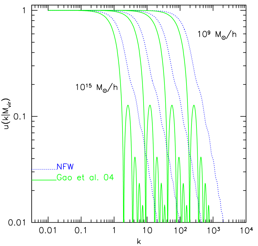
Figure 3: Fourier transform of the density profile. The dotted curves show the analytic Fourier transform of the NFW profile of different host-halo masses: $10^{15}$, $10^{13}$, $10^{11}$ and $10^{9}\,M_{\odot}/h$. The solid curves show the numerical Fourier transform of the Gao et al. (2004) substructure density distribution. The mass-concentration relation by Zhao et al. (2009) was adopted here.

2.2.3 Mass-concentration relation

The final ingredient we need to model is the mass-concentration relation for the substructures. In the top-left panel of Fig. 1, we show the mass-concentration relation fit to the substructures in the Aquarius simulation (Springel et al., 2008) by Pieri et al. (2009),

$$c_{sub}(m,d_{vir})=d_{vir}^{-\alpha_{R}}\left[c_{1}\;m_{sub}^{-\alpha_{c_{1}}}+c_{2}\;m_{sub}^{-\alpha_{c_{2}}}\right]\,.$$ (16)

Here, $d_{vir}=r/R_{vir}$ is the distance from the host-halo centre in units of the virial radius. The parameters are listed in Tab. 2 of Pieri et al. (2009) for haloes $200$ times denser than the background. In the figure, we plot the mass-concentration relation for clumps at $10\%$ and $100\%$ of the virial radius. This proposed relation takes into account that substructures with the same mass are more concentrated if they are closer to the host-halo centre, which is necessary for their survival. To be consistent with our choice of the virial overdensity, we have normalized this distribution to $\Delta_{vir}$. Since for subclumps at the virial radius ($d_{vir}=1$), the fit (16) follows the mass-concentration relation of isolated haloes and increases with decreasing distance from the host-halo centre, we adopt for each model

$$c_{sub}(m,d_{vir})=d_{vir}^{-\alpha_{R}}c_{vir}^{I}\;,$$ (17)

where $I=$N, S, or Z, corresponding to C1, C2 and C3 (see Eqs. 6, 7, 8 and 16).

2.3 Summary

Before we proceed, let us briefly summarize the main ingredients of our extension to the halo model.

• The abundance and bias of host haloes are taken from Sheth & Tormen (1999).

• Host haloes and subhaloes are assumed to have NFW density profiles.

• We study deterministic (D1) and stochastic (D2) models of halo concentration at fixed mass, and explore three different choices for the mean relation between mass and concentration (C1, C2, C3).

• We study two choices for the density run of subhaloes around the center of the host: either it is the same NFW profile as the smooth component (S1), or it has the form suggested by Gao et al. (2004) (S2).

• The mass function of subhalos is given by equation (2.2.1), found in and normalized to numerical simulations.

• The concentration of subhaloes increases towards the centre of their host halo, in agreement with numerical simulations (Pieri et al., 2009). As we describe below, our halo model includes this effect only rather crudely.

3 Non-linear power spectrum

In this Section, we describe the halo-model approach at the non-linear dark-matter power spectrum and study how it changes at small scales when different models for the mass-concentration relation are taken into account. We will also show how the non-linear power spectrum can be decomposed when a realistic model for the substructure mass function in host haloes and two models for their spatial distribution are taken into account. The formalism for the substructure contribution to the one-halo term of the non-linear dark-matter power spectrum has been developed by Sheth & Jain (2003). Here, we shall also consider the clump contributions to the two-halo term and show the relevant equations.

3.1 Contributions from host haloes

In the halo model approach (Scherrer & Bertschinger, 1991; Seljak, 2000; Scoccimarro et al., 2001; Cooray & Sheth, 2002), the two-point dark-matter correlation function is

$$\xi(\vec{x}-\vec{x}^{\prime})=\xi_{1H}(\vec{x}-\vec{x}^{\prime})+\xi_{2H}(\vec{x}-\vec{x}^{\prime})\;,$$ (18)

where the first or Poisson term describes the contribution to the matter density from individual haloes, while the second term describes the contribution from halo correlations. While both terms require knowledge of the halo mass function and their dark-matter density profiles, the second needs also the two-point correlation function of haloes of different mass $\xi_{hh}(r|M_{1},M_{2})$. Since the two-point correlation function on large scales is dominated by the two-halo term and has to follow the linear correlation function, a good and convenient way to express the two-halo correlation function is

$$\xi_{hh}(r|M_{1},M_{2})\approx b(M_{1})b(M_{2})\xi_{lin}(r)\,.$$ (19)

In view of later convolutions, it is convenient to work in Fourier space. We then define the dark matter power spectrum $P(k,z)$ as

$$P(k,z)=4\pi\int\xi(r,z)\frac{\sin(kr)}{kr}r^{2}{\rm d}r\,.$$ (20)

For further convenience, and as is common in the large scale structure community, we define the dimensionless quantity

$$\Delta^{2}(k,z)\equiv\frac{k^{3}P(k,z)}{2\pi^{2}}\,.$$ (21)

The dark matter power spectrum can be decomposed as

$$P(k,z)=P_{1H}(k,z)+P_{2H}(k,z)$$ (22)

where

$$P_{1H}(k,z) = \int\left(\dfrac{M}{\bar{\rho}}\right)^{2}n(M,z)$$ (23)

$$\times \int p(c|M)u^{2}(k|c(M))\mathrm{d}c\,\mathrm{d}M,$$

and

$$P_{2H}(k,z) = P_{\rm lin}(k)\Big{[}\int\dfrac{M}{\bar{\rho}}n(M,z)\,b(M,z)$$ (24)

$$\times \int p(c|M)\,u(k|c,M)\,\frac{b(c,M,z)}{b(M,z)}\,\mathrm{d}c\,\mathrm{d}M\Big{]}^{2}$$

are the one- and two-halo contributions. Here, $b(c,M,z)$ is the bias factor with respect to the dark-matter of halos of mass $M$ at $z$ having concentration $c$. The dependence of halo bias on $c$ as well as $M$ is a simple way of including the ‘assembly bias’ effect in the model. In practice, we ignore this effect, meaning that we set $b(c,M,z)/b(M,z)=1$ from now onwards. Note that the integrals extend over all collapsed masses.

The most commonly used approximations in the literature (Seljak, 2000; Cooray & Sheth, 2002) use the deterministic model D1 for the concentration distribution and consider steep models for the mass-concentration relation in order to not loose small scale power.

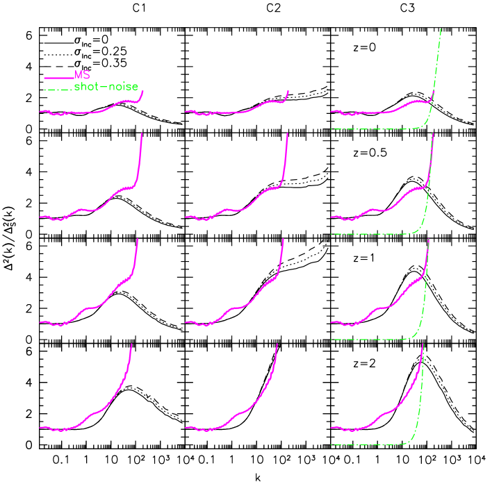
Figure 4: Ratio of the non-linear power spectrum predicted by the halo model and the fit by Smith et al. (2003). From left to right, the panels show results for the three models of the mass-concentration relation, as described in the text. From top to bottom, we show results at four different redshifts. In all panels, solid curves show the ratio for the deterministic concentration assignment, while dotted and dashed curves refer to the stochastic model with widths $\sigma_{\ln c}=0.25$ and $0.35$. The heavy solid curves show the ratio between the power spectrum in the Millennium Simulation and Smith et al. (2003) at the corresponding redshifts, and the dash-dotted line (only in the right panels) shows the shot noise in the MS with respect to the fit.

In Fig. 4 we show the non-linear dark-matter power spectrum predicted using the halo model, as described above, divided by the power-spectrum fit by Smith et al. (2003) at four different redshifts (from top to bottom) and assuming three models for the mass-concentration relation (from left to right). The solid curve refers to the analytical non-linear power spectrum with the deterministic concentration model (D1), while the dotted and dashed curves refer to the model which adopt the stochastic model (D2) with widths $\sigma_{\ln c}=0.25$ and $0.35$, respectively. The ringing of the curves for large $k$ is due to the Fourier tranform of the density profile. The thick solid curve refers to the power spectrum measured in the Millennium Simulation (Springel et al., 2005; Boylan-Kolchin et al., 2009). The dotted-dashed line in the right panels shows the shot-noise limit in the Millennium Simulation, which we do not remove from the numerical power spectrum, at the corresponding redshifts.

From the Figure, we notice that model C1 reproduces the MS power spectrum quite well up to $k\approx 10$, while model C2 performs better. Model C3 is also quite accurate and does not decrease at small scales, although it somewhat overestimates the power in the range $1\lesssim k\lesssim 50$. Note that the stochastic concentration model (D2) increases the power on small scales ($k\gtrsim 10$) by 15 to 20% compared to the deterministic (D1) case.

3.2 Contributions from subhaloes

Figure 5: Top: Ratio of the 1-halo components divided into substructures (Eqs. ($1$), 26, ($3$) and ($4$)) compared to the 1-halo term (Eq. 23). A width of $\sigma_{\ln c}=0.25$ was assumed in the concentration distribution. In the left and right panels, we adopt the NFW and the Gao et al. (2004) model for the substructure distribution. Bottom: Ratio of the 2-halo components (Eqs. 32, 33 and 34) compared to the 2-halo term (Eq. 24).

Considering the contribution from substructures, the 1-halo term can be further decomposed into four contributions from the mutual correlations between smooth and clump components as explained in what follows.

• Smooth-smooth correlation:

  $$P_{1H,ss}(k,z) = \int\left(\dfrac{M}{\bar{\rho}}\right)^{2}n(M,z)$$

  $$\times \int\left(\dfrac{M_{sm}}{M}\right)^{2}u^{2}(k|c(M_{sm}))p(c|M)\mathrm{d}c\,\mathrm{d}M$$

• Smooth-clump correlation:

  $$P_{1H,sc}(k,z) = 2\int\left(\dfrac{M}{\bar{\rho}}\right)^{2}n(M,z)\int\dfrac{M_{sm}}{M}u(k|c(M_{sm}))\,$$ (26)

  $$\times U_{s}(k|c(M))\mathcal{I}_{c(M)}(k,z)p(c|M)\mathrm{d}c\,\mathrm{d}M$$

• Two-point correlation between different clumps in the same halo:

  $$P_{1H,cc}(k,z) = \int\left(\dfrac{M}{\bar{\rho}}\right)^{2}n(M,z)$$

  $$\times \int U^{2}_{s}(k|c(M))\,\mathcal{I}^{2}_{c(M)}(k,z)p(c|M)\mathrm{d}c\,\mathrm{d}M$$

• Two-point correlation between pairs in the same clump:

  $$P_{1H,self-c}(k,z) = \int\left(\dfrac{M}{\bar{\rho}}\right)^{2}n(M,z)$$

  $$\times \int\mathcal{J}_{c(M)}(k,z)p(c|M)\mathrm{d}c\,\mathrm{d}M$$

Here, we define the smooth mass as

$$M_{sm}=(1-f_{s})\,M,$$ (29)

which depends on the host halo concentration (see eq. 2.2.1), while $\mathcal{I}$ and $\mathcal{J}$ are the functions

$$\mathcal{I}_{c(M)}(k,z)=\int_{0}^{M}\dfrac{m}{M}\int u_{m}(k,c)\frac{\mathrm{d}N(c(M),z)}{\mathrm{d}m}p(c|M)\mathrm{d}c\,\mathrm{d}m$$ (30)

and

$$\mathcal{J}_{c(M)}(k,z)=\int_{0}^{M}\left(\dfrac{m}{M}\right)^{2}\int u^{2}_{m}(k,c)\frac{\mathrm{d}N(c(M),z)}{\mathrm{d}m}p(c|M)\mathrm{d}c\,\mathrm{d}m\,,$$ (31)

where we also take into account the scatter in at fixed mass in the subhalo mass-concentration relation when the stochastic model is considered. The subhalo concentration depends on its mass and also on its radial distance from the host halo centre (see eq.17). The mass-concentration relation adopted is consistent with the one assumed for isolated host haloes, such that the subhalo mass-concentration relation, for distance larger then the virial radius of the host follows the halo mass-concentration relation. To account for the radial distance dependance we randomly sample the substructure density profile distribution in the host, consistently with the model adopted (NFW or Gao et al. (2004)), and locate the subhalo at a distance $d_{vir}$ from the host centre ($d_{vir}$ is expressed in unit of the host halo virial radius). Note that we do not consider scatter in $f_{s}$ at fixed $c$ and $M$.

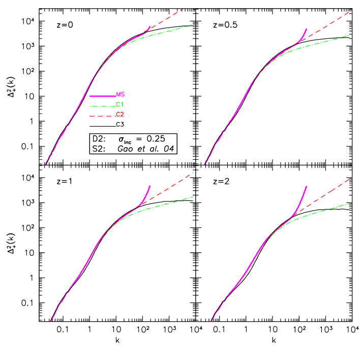
Figure 6: Non-linear dark-matter power spectrum, with substructures, at four different redshifts. We show three models referring to different mass-concentration relations. The heavy solid line shows the data from the Millennium Simulation. The width of the concentration distribution is assumed to be $\sigma_{\ln c}=0.25$, and the substructure distribution in the host halo is modeled according to Gao et al. (2004). For all models, the mass distribution in both the host haloes and in their substructures follows the NFW profile.

Likewise, the large-scale (2-Halo) term can be further decomposed according to the different correlations between smooth and clump components. In this case, we have the three contributions

• Smooth-smooth component correlation on large scales:

  $$P_{2H,ss}(k,z)=P_{lin}(k){\mathcal{S}^{I}}^{2}(k,z)$$ (32)

• Smooth-clump correlation:

  $$P_{2H,sc}(k,z)=2P_{lin}(k)\mathcal{S}^{I}(k,z)\mathcal{C}^{I}(k,z)\,$$ (33)

• Clump correlation:

  $$P_{2H,cc}(k,z)=P_{lin}(k){\mathcal{C}^{I}}^{2}(k,z)$$ (34)

Here,

$$\mathcal{S}^{I}(k,z) = \int\dfrac{M}{\bar{\rho}}n(M,z)b(M,z)$$ (35)

$$\times \int\dfrac{M_{sm}}{M}u(k,c(M_{sm}))p(c|M)\mathrm{d}c\,\mathrm{d}M,$$

and

$$\mathcal{C}^{I}(k,z) = \int\dfrac{M}{\bar{\rho}}n(M,z)b(M,z)$$ (36)

$$\times \int\mathcal{I}_{c(M)}(k,z)U_{s}(k|c(M))p(c|M)\mathrm{d}c\,\mathrm{d}M.$$

Recall that $I=$ N,S, or Z, corresponding to C1, C2 and C3 (see Eqs. 6, 7, 8 and 16).

The full non-linear dark-matter power spectrum is the sum of all components,

$$P_{+}(k,z)=\sum_{i=1}^{4}P_{1H,i}(k,z)+\sum_{i=1}^{3}P_{2H,i}(k,z)\,.$$ (37)

In Fig. 5 we show the ratio of the individual contributions to the 1- and 2-halo components. We set the width $\sigma_{\ln c}=0.25$ for the concentration distribution, and adopt C3 for the mass-concentration relations. All functions depending on the concentration are estimated by marginalizing over $c$. Models S1 and S2 for the subclump distribution within the host are adopted in the different panels. Note that in both the 1- and 2-halo terms, the dominant contribution is due to pairs in which both members are in the smooth component; smooth-clump and clump-clump pairs never contribute more than 10% of the signal, and they become even less dominant at large $k$. The transition scale is around $k\approx 1$, since it represents the size of a typical collapsed halo in which the clumps are located. For $k\gtrsim 1$ the smooth-clump and clump-clump terms start to drop down due to the density profile distribution of subhaloes in the host system. In other words, for scale smaller then 1 Mpc $h^{-1}$ the two-point probability has a threshold due to the typical distribution scale of the clumps within the virial radius of the host. Comparing right and left panels we notice that the power-spectrum components are quite sensitive to the more rapid decrease of the Fourier transform model S2 (right panels) compared to model S1 (left panels), both in the 1-Halo and the 2-Halo terms. However, the contribution from pairs within the same subclump (self-clump) increases with $k$ reaching values of order $50\%$ at $k\approx 10^{4}$, this is due to the matter density profile distribution in small clumps, more and more concentrated as their mass decrises. The probability to find a pair of points of the same clump becames larger and larger as the scale decreases – so for large value of $k$.

In Fig. 6, we show the full non-linear power spectrum at four different redshifts. We include results for models C1, C2 and C3 and for $\sigma_{\ln c}=0.25$. We adopt the NFW profile for the matter-density distribution in both the host haloes and their substructures, and model S2 for the radial subclump distribution within the host haloes.

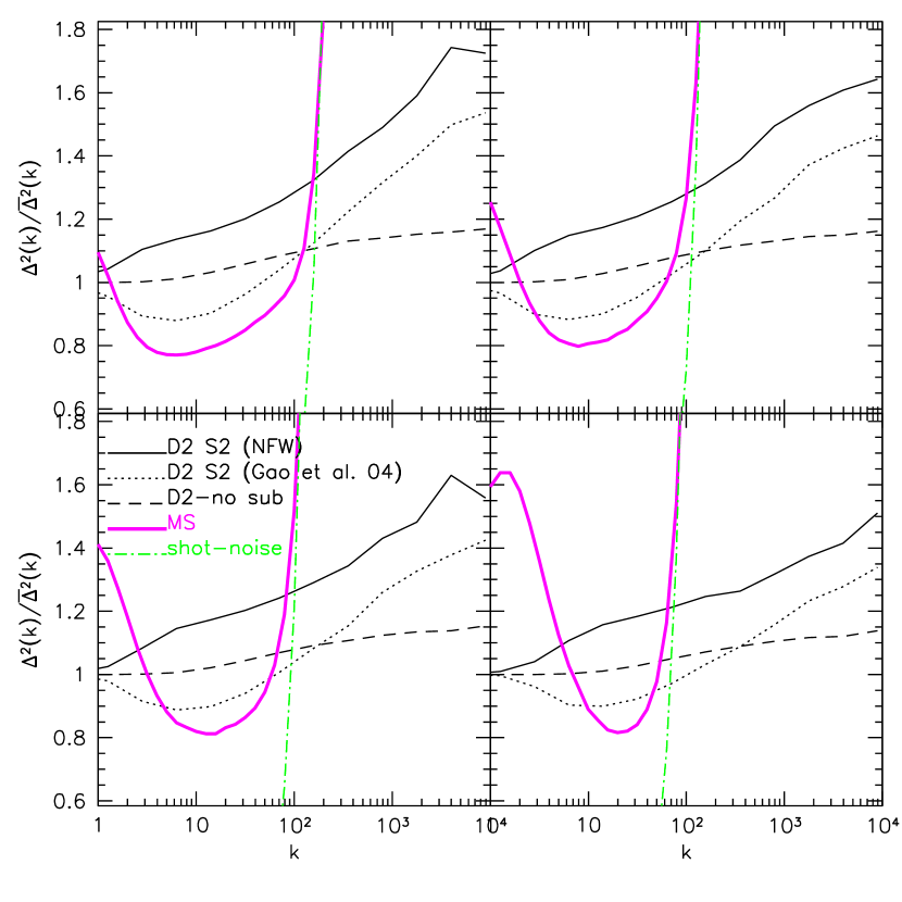
Figure 7: Ratio between the predicted power-spectrum in our extension of the halo model, which includes substructures and the stochastic assignment of halo concentrations, to the power spectrum in the standard implementation of the halo model, which ignores halo substructures and assigns concentrations deterministically. For the log-normal scatter in concentration we adopt $\sigma_{\ln c}=0.25$. The solid and dotted curves assume an NFW or a Gao et al. (2004) model for the subclump distribution. The dashed line shows the predicted ratio when we allow scatter in the concentrations but assume smooth halos with no substructure. The thick magenta line shows the power-spectrum ratio for the Millennium Simulation and the dash-dotted line shows the shot-noise.

In Fig. 7 we show the ratio between the full non-linear power spectrum with $\sigma_{\ln c}=0.25$, considering models S1 (solid) and S2 (dotted), and the standard halo model – 1 and 2-Halo terms and no scatter in concentration, at four different redshifts as in Figure 6. This figure quantifies the importance of substructures and the concentration scatter in the halo model. Including both effects increases the small-scale power by $\approx 30\%$. On the large scales where the 2-Halo term dominates, accounting for or ignoring substructure makes no difference, as expected (Sheth & Jain, 2003). In the figure we also show the ratio between the power spectra in the MS (thick solid line) and the standard halo model with stochastic concentration assignment (dashed line), compared to the standard halo model without concentration scatter. The dash-dotted line show the shot-noise.

4 Cross correlations

We now describe halo models of the cross correlation between haloes and mass, as well as between substructures and mass. We shall show that while the cross correlation with the smooth component dominates the signal on large scales, the self-cross correlation dominates on small scales. We shall also quantify the scales on which different host-halo masses and substructures contribute significantly. In contrast to Hayashi & White (2008), who presented a simple model for the auto- and cross-correlation functions, we study all contributions to the non-linear power spectrum explicitly. As for the power-spectrum in the previous section, our model of the 1-halo term follows Sheth & Jain (2003).

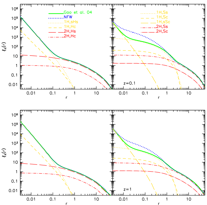
Figure 8: Halo and subhalo-mass cross-correlations at redshift $z=0.1$ (top) and $z=1$ (bottom). In each panel, we show the contributions of haloes and substructures to the 1- and 2-halo terms. The left and right panels show the cross-correlation between haloes and mass and between substructures and mass, respectively. We adopt the Gao et al. (2004) model for the radial subclump distribution in the host halo, Zhao et al. (2009) for the mass-concentration relation and $\sigma_{\ln c}=0.25$ for its width. The heavy solid curve shows the sum of all contributions. For comparison, we also show in each panel the total cross-correlation function when the spatial distribution of subclumps in the host follows the NFW model (heavy-dotted curve).

4.1 Cross-correlation of haloes and mass

We begin by writing down the contributions to the 1-halo term of the cross-correlation power spectrum between haloes and matter. Sitting at the center of a host halo, and assuming that the matter is divided into smooth and clumpy components, the halo-smooth self-correlation and the halo-clump cross-correlation can be written as

$$P^{\times}_{1H,sHs}(k,z) = \int\dfrac{M}{\bar{\rho}}n(M,z)$$ (38)

$$\times \int\dfrac{M_{sm}}{M}u(k|c(M_{sm}))p(c|M)\mathrm{d}c\,\mathrm{d}M,$$

and

$$P^{\times}_{1H,Hc}(k,z) = \int\dfrac{M}{\bar{\rho}}n(M,z)$$ (39)

$$\times \int U_{s}(k,c)\mathcal{I}_{c(M)}(k,z)p(c|M)\mathrm{d}c\,\mathrm{d}M.$$

We recall that $M_{sm}$ is the smooth mass of the host halo, $u(k|c(M_{sm}))$ and $U_{s}(k|c(M))$ are the Fourier transforms of the density profiles of the smooth component and of the clump distribution respectively. Moreover, $n(M,z)$ is the halo mass function at redshift $z$ and $\mathcal{I}_{c(M)}$ is given by Eq. (30).

Regarding the contributions to large scales (the 2-halo term), we start from the same idea, i.e. we imagine sitting at the center of a host halo and cross-correlate with the smooth and the clumpy components of a distant halo. However, in this case we also have to take the halo bias relative to the dark matter distribution into account, as well as the non-linear dark-matter power spectrum. The smooth and clump cross-correlation power spectra are

$$P^{\times}_{2H,Hs}(k,z)=\frac{P_{lin}(k,z)}{\bar{n}_{h}}\int n(M,z)b(M,z)\mathrm{d}M\mathcal{S}^{I}(k,z)$$ (40)

and

$$P^{\times}_{2H,Hc}(k,z)=\frac{P_{lin}(k,z)}{\bar{n}_{h}}\int n(M,z)b(M,z)\mathrm{d}M\mathcal{C}^{I}(k,z),$$ (41)

with $\mathcal{S}^{I}$ and $\mathcal{C}^{I}$ given by Eqs. (35) and (36).

4.2 Cross-correlation of subhaloes and mass

Let us now place ourselves at the center of a clump and determine the cross-correlation on small scales. In this case, the 1-halo term will be the sum of three components: (i) the self-correlation with the substructure mass; (ii) the cross-correlation with the mass in the other substructures contained in the same host halo, and (iii) the cross-correlation with the smooth component. These three terms are

$$P^{\times}_{1H,Ss}(k,z) = \frac{1}{\bar{n}_{s}}\int\dfrac{M}{\bar{\rho}}n(M,z)\int\dfrac{M_{sm}}{M}u(k|c(M_{sm}))$$ (42)

$$\times U_{s}(k|c(M))N_{s}(c(M),z)p(c|M)\mathrm{d}c\,\mathrm{d}M,$$

further

$$P^{\times}_{1H,Sc}(k,z) = \frac{1}{\bar{n}_{s}}\int\dfrac{M}{\bar{\rho}}n(M,z)\int U^{2}_{s}(k|c(M))$$ (43)

$$\times \mathcal{I}_{c(M)}(k,z)N_{s}(c(M),z)p(c|M)\mathrm{d}c\,\mathrm{d}M$$

and

$$P^{\times}_{1H,sSc}(k,z)=\int\dfrac{M}{\bar{\rho}}n(M,z)\int\mathcal{I}_{c(M)}(k,z)p(c|M)\mathrm{d}c\,\mathrm{d}M,$$ (44)

where we have underlined that $N_{s}$, the number of substructures in a $M$-halo, depends on the mass through the concentration and on redshift. For the 2-halo term, we have two equations analogous to those of the halo-matter cross-correlation, and we need to integrate over the substructure mass function. We find

$$P^{\times}_{2H,Ss}(k,z) = \frac{P_{lin}(k,z)}{\bar{n}_{s}}\int n(M,z)b(M,z)\int N_{s}(c(M),z)$$ (45)

$$\times U_{s}(k|c(M))p(c|M)\mathrm{d}c\,\mathrm{d}M\,\mathcal{S}^{I}(k,z),$$

and

$$P^{\times}_{2H,Sc}(k,z) = \frac{P_{lin}(k,z)}{\bar{n}_{s}}\int n(M,z)b(M,z)\int N_{s}(c(M),z)$$ (46)

$$\times U_{s}(k|c(M))p(c|M)\mathrm{d}c\,\mathrm{d}M\,\mathcal{C}^{I}(k,z).$$

We show the results in real space for each component of the cross-correlation after the inverse Fourier transform

$$\xi_{i,\times}(r,z)=\frac{1}{2\pi^{2}}\int P_{iH,k}(k,z)\frac{\sin(kr)}{kr}k^{2}\mathrm{d}k\;,$$ (47)

where the index $i$ runs over all halo and substructure cross-correlation terms. Going from Fourier to real space, some of the 1-halo terms are simple, because we are inverse Fourier transforming the NFW density profile and the density run of subclumps in the host (see eq. 15). For the model S1, in which subclumps follow the dark matter distribution, terms like $uU_{s}$ are the convolution of two NFW profiles, so they can also be written analytically (Sheth et al., 2001).

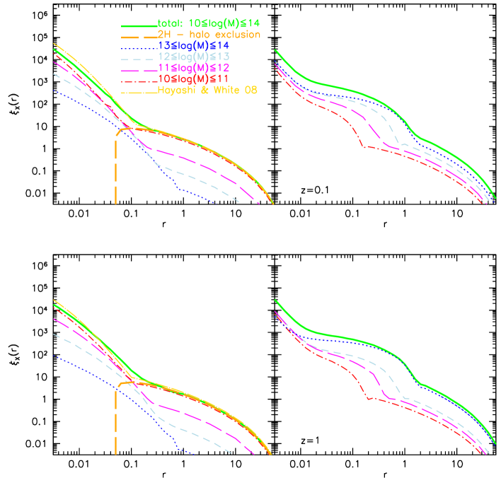
Figure 9: Halo and subhalo-mass cross-correlations at $z=0.1$ and $z=1$ separating the contributions from different host-halo masses. The left panels show the halo-mass cross-correlation. The 2-halo terms in different mass bins have been normalized to the total number of haloes between $10^{10}$ and $10^{14}\,M_{\odot}/h$. The right panels show the subhalo-mass cross-correlation considering clumps in different host-halo masses. The curves in this case have been normalized to the mean number of clumps in haloes with mass from $10^{10}$ and $10^{14}\,M_{\odot}/h$.

In Fig. 8, we show the cross-correlation between haloes and matter (left panels) as well as between substructures and matter (right panels) at the two different redshifts $z=0.1$ and $z=1$. These represent the mean redshifts of galaxies in the SDSS (Adelman-McCarthy et al., 2006; Wang et al., 2007) and in typical weak-lensing surveys, respectively. In the left panels, we show the halo-matter cross-correlation function considering the two components both in the 1- and 2-halo terms. We adopt models C3, D2 with $\sigma_{lnc}=0.25$ and S2. The solid and dotted curves show the total cross-correlation, with distributions S1 and S2 for placing substructures in the host halo. Notice that, in the host mass cross-correlation, the latter choice does not influence the total. On the other hand, the cross-correlation between substructures and mass is sensitive to the choice of the radial subclump distribution. In the right panels, we show the cross correlation between clump and mass. Here, too, we show the three components of the 1-halo term and the two components of the 2-halo term. The solid and dotted curves are, respectively, the total predicted signal using models S1 and S2. From the figure we notice that substructures contribute a signature on scales of order $30$ kpc or so.

In the left panels of Fig. 9, we show the cross-correlation function between haloes and matter, splitting the contributions into different host-halo mass bins. The integrals in Eqs. (38, 39, 40) and (41) have been performed between the lower and upper bounds of each bin, while $\mathcal{S}^{I}(k,z)$ and $\mathcal{C}^{I}(k,z)$ have been integrated over all masses. The solid line shows the total power spectrum from haloes in the entire mass range, i.e. between $10^{10}$ and $10^{14}\,M_{\odot}/h$. The curves are normalized to the mean number of haloes in the entire range.

The long-dashed-dotted curve in the left panels, shows the model of Hayashi & White (2008). In their model the 1-halo term is due to the dark matter density profile of the host halo, while the two halo term by the product between bias factor and the mass autocorrelation function predicted by the linear theory. In their model we consider the mean mass predicted by the Sheth & Tormen (1999) mass function between $10^{10}$ and $10^{14}\,M_{\odot}/h$.

In the right panels, we show the substructure-mass cross-correlation considering clumps in the same host-halo mass bins. These curves have been normalized by the mean number of clumps in haloes between $10^{10}$ and $10^{14}\,M_{\odot}/h$. In this case, showing the predicted contribution from different mass bins, we account for halo exclusion in the halo-mass cross correlation. An accurate treatment of halo exclusion may be numerically tedious. Here, we adopt an approximate approach in which the 2-halo term vanishes on scales smaller than the virial radius of the mean mass in the bin considered (see e.g. (Cacciato et al., 2009) for a similar approach in the galaxy-dark matter cross-correlation). Thus, if $M_{1}$ and $M_{2}$ are the lower and upper bounds of the bin, we can write

$$1+\xi^{h-excl}_{2H}(r|M_{1},M_{2})\approx\left[1+\xi_{2H}(r|M_{1},M_{2})\right]\times W(r|R_{vir})\,$$ (48)

where $R_{vir}$ is the virial radius of the mean mass between $M_{1}$ and $M_{2}$ which is used as a typical cut-off scale of the 2-halo cross-correlation signal here. $W(r|R_{vir})$ is a window function equal to $1$ if $r>R_{vir}$ and $0$ for $r\leq R_{vir}$.

The curves in the left panels of Fig. 9 account for this effect. The signal near the transition between the 1- and 2-halo terms is reduced by $30\%$ due to halo exclusion. The heavy dashed line shows the total 2-halo term between $10^{10}$ and $10^{14}\,M_{\odot}/h$, taking halo exclusion into account. The curve tends to zero at a scale corresponding to the virial radius of a $10^{10}\,M_{\odot}/h$ halo. The 2-halo term integrals have been divided into different bins, for each of which we assign a cut-off scale corresponding to the virial radius of a mean halo. To estimate the total signal from haloes between $10^{10}$ and $10^{14}\,M_{\odot}/h$ we sum the contributions from the individual mass bins. In the clump-mass cross-correlation, we ignore the halo exclusion since the transition between the 1- and the 2-halo contributions occurs at larger scales, hence the exclusion will not change the signal at all.

5 Summary and Conclusions

We have shown how the halo-model formalism can be extended to account for scatter in halo concentration at fixed mass, and for the presence of substructures in dark matter haloes. Differences in the mass-concentration relation do affect the predicted non-linear power spectrum. We quantified this by considering three models for the $M$-$c$ relation, as well as a deterministic and a stochastic models for the concentration at fixed mass. Accounting for substructure means that the 1-halo and 2-halo terms should be written as sums of four and three types of pairs, respectively. If one uses realistic models for these different pair-types, then the halo model calculation is in reasonable agreement with the non-linear power spectrum measured in the Millennium Simulation, over a range of redshifts.

The cross-correlation between halos and mass can also be estimated using the halo-model formalism. We have shown how, also in this case, substructures can be taken into account and how the cross-correlation signal between clumps and mass can be split into different contributions.

The agreement with simulations is not yet at the percent level, so there is room for improvement. The simulations show an excess at around $k\sim 1$ relative to our model – this is almost certainly not due problems with our substructure calculation, since it is on larger scales than those on which substructures dominate. The discrepancy is also unlikely to be due to our decision to ignore ‘assembly bias’ effects. Rather it may be due to the fact that our 2-halo term is too crude – on these smaller scales, one must include the effects of nonlinear bias, perhaps following Smith et al. (2007).

• Our formulation of the halo model assumes that the mass fraction in substructures is a deterministic function of the halo concentration: in practice, there is a distribution of $f_{s}$ values at fixed $c$ and $M$. Allowing for this stochasticity simply adds one more integral in most of our expressions, that can matter at the percent level on the small scales of interest here (for essentially the same reason that scatter in $c$ and fixed $M$ matters at the ten percent level on small scales).

• We only include some of the effects of the known correlation between subhalo concentration and distance from the center of the host. Specifically, our current implementation accounts for the fact that the spatial dependence means subhalo concentrations (at fixed mass) are stochastic, but it does not include the fact that this is correlated with distance from host halo center. Implementing a spatially dependent concentration is difficult in Fourier space, so doing so in configuration is probably the best way forward.

• We also do not account for the fact that subhalos themselves have substructure. This will matter most for the contribution which comes from pairs which are in the same subhalo (for the same reason that substructure is not important for the 2-halo term).

• Halo exclusion matters for the cross-correlation signal. There are exclusion effects associated with the subhalos too, which we currently ignore.

• Although the sum of the smooth and clumpy components should give an NFW profile, our current implementation assumes the smooth component follows and NFW profile, whereas the clumpy one does not. Hence there is no guarantee that the sum of the two actually is NFW at high precision. While this is relatively easy to fix (simply define the profile of the smooth component to be the required NFW minus the clumpy component), we have not done so.

• And finally, at this level of precision, halo shapes also matter. In particular, the distribution of $f_{s}$ and $c$ at fixed $M$ may depend on halo shape – once this has been quantified in simulations, it may become necessary to extend our formalism to include shapes.

The formalism presented in this paper can be used in subsequent studies to make more realistic predictions for the galaxy-galaxy lensing signals and for the lensing convergence power spectrum. By identifying the different contributions due to the smooth and clumpy components of the dark-matter haloes, this will also allow us to quantify the contributions the convergence power spectrum not just by different halo masses, but also by different substructures.

References

- Adelman-McCarthy et al. (2006) Adelman-McCarthy J. K., Agüeros M. A., Allam S. S., Anderson K. S. J., Anderson S. F., Annis J., Bahcall N. A., Baldry I. K., Barentine J. C., et al. 2006, ApJS, 162, 38
- Allgood et al. (2006) Allgood B., Flores R. A., Primack J. R., Kravtsov A. V., Wechsler R. H., Faltenbacher A., Bullock J. S., 2006, MNRAS, 367, 1781
- Angulo et al. (2009) Angulo R. E., Lacey C. G., Baugh C. M., Frenk C. S., 2009, MNRAS, 399, 983
- Bacon et al. (2006) Bacon D. J., Goldberg D. M., Rowe B. T. P., Taylor A. N., 2006, MNRAS, 365, 414
- Bartelmann & Schneider (2001) Bartelmann M., Schneider P., 2001, Physics Reports, 340, 291
- Bond et al. (1991) Bond J. R., Cole S., Efstathiou G., Kaiser N., 1991, ApJ, 379, 440
- Boylan-Kolchin et al. (2009) Boylan-Kolchin M., Springel V., White S. D. M., Jenkins A., Lemson G., 2009, MNRAS, 398, 1150
- Bryan & Norman (1998) Bryan G. L., Norman M. L., 1998, ApJ, 495, 80
- Bullock et al. (2001) Bullock J. S., Kolatt T. S., Sigad Y., Somerville R. S., Kravtsov A. V., Klypin A. A., Primack J. R., Dekel A., 2001, MNRAS, 321, 559
- Cacciato et al. (2009) Cacciato M., van den Bosch F. C., More S., Li R., Mo H. J., Yang X., 2009, MNRAS, 394, 929
- Colless et al. (2001) Colless M., Dalton G., Maddox S., Sutherland W., Norberg P., Cole S., Bland-Hawthorn J., Bridges T., Cannon R., et al. 2001, MNRAS, 328, 1039
- Cooray & Sheth (2002) Cooray A., Sheth R., 2002, Physics Reports, 372, 1
- De Lucia et al. (2004) De Lucia G., Kauffmann G., Springel V., White S. D. M., Lanzoni B., Stoehr F., Tormen G., Yoshida N., 2004, MNRAS, 348, 333
- Diemand et al. (2007) Diemand J., Kuhlen M., Madau P., 2007, ApJ, 667, 859
- Dolag et al. (2004) Dolag K., Bartelmann M., Perrotta F., Baccigalupi C., Moscardini L., Meneghetti M., Tormen G., 2004, A&A, 416, 853
- Duffy et al. (2008) Duffy A. R., Schaye J., Kay S. T., Dalla Vecchia C., 2008, MNRAS, 390, L64
- Eisenstein & Hu (1998) Eisenstein D. J., Hu W., 1998, ApJ, 496, 605
- Eke et al. (1996) Eke V. R., Cole S., Frenk C. S., 1996, MNRAS, 282, 263
- Faltenbacher & White (2010) Faltenbacher A., White S. D. M., 2010, ApJ, 708, 469
- Gao et al. (2008) Gao L., Navarro J. F., Cole S., Frenk C. S., White S. D. M., Springel V., Jenkins A., Neto A. F., 2008, MNRAS, 387, 536
- Gao et al. (2005) Gao L., Springel V., White S. D. M., 2005, MNRAS, 363, L66
- Gao et al. (2004) Gao L., White S. D. M., Jenkins A., Stoehr F., Springel V., 2004, MNRAS, 355, 819
- Ghigna et al. (2000) Ghigna S., Moore B., Governato F., Lake G., Quinn T., Stadel J., 2000, ApJ, 544, 616
- Giocoli et al. (2008) Giocoli C., Pieri L., Tormen G., 2008, MNRAS, 387, 689
- Giocoli et al. (2010) Giocoli C., Tormen G., Sheth R. K., van den Bosch F. C., 2010, MNRAS, 404, 502
- Giocoli et al. (2008) Giocoli C., Tormen G., van den Bosch F. C., 2008, MNRAS, 386, 2135
- Governato et al. (1999) Governato F., Babul A., Quinn T., Tozzi P., Baugh C. M., Katz N., Lake G., 1999, MNRAS, 307, 949
- Green et al. (2004) Green D. A., Tuffs R. J., Popescu C. C., 2004, MNRAS, 355, 1315
- Guzzo et al. (2000) Guzzo L., Bartlett J. G., Cappi A., Maurogordato S., Zucca E., Zamorani G., Balkowski C., Blanchard A., Cayatte V., Chincarini G., Collins C. A., Maccagni D., MacGillivray H., Merighi R., Mignoli M., Proust D., et al. 2000, A&A, 355, 1
- Hagan et al. (2005) Hagan B., Ma C., Kravtsov A. V., 2005, ApJ, 633, 537
- Hayashi et al. (2007) Hayashi E., Navarro J. F., Springel V., 2007, MNRAS, 377, 50
- Hayashi & White (2008) Hayashi E., White S. D. M., 2008, MNRAS, 388, 2
- Jenkins et al. (2001) Jenkins A., Frenk C. S., White S. D. M., Colberg J. M., Cole S., Evrard A. E., Couchman H. M. P., Yoshida N., 2001, MNRAS, 321, 372
- Jing (1998) Jing Y. P., 1998, ApJL, 503, L9+
- Jing (2000) Jing Y. P., 2000, ApJ, 535, 30
- Jing & Suto (2002) Jing Y. P., Suto Y., 2002, ApJ, 574, 538
- Kauffmann et al. (1999) Kauffmann G., Colberg J. M., Diaferio A. White S. D. M., 1999, MNRAS, 303, 188
- Kitayama & Suto (1996) Kitayama T., Suto Y., 1996, MNRAS, 280, 638
- Lacey & Cole (1993) Lacey C., Cole S., 1993, MNRAS, 262, 627
- Macciò et al. (2008) Macciò A. V., Dutton A. A., van den Bosch F. C., 2008, MNRAS, 391, 1940
- Mandelbaum et al. (2005) Mandelbaum R., Tasitsiomi A., Seljak U., Kravtsov A. V., Wechsler R. H., 2005, MNRAS, 362, 1451
- Meneux et al. (2009) Meneux B., Guzzo L., de La Torre S., Porciani C., Zamorani G., Abbas U., Bolzonella M., Garilli B., Iovino A., Pozzetti L., Zucca E., Lilly S. J., Le Fèvre O., Kneib J., Carollo C. M., Contini T., Mainieri V., et al. 2009, A&A, 505, 463
- Mo & White (1996) Mo H. J., White S. D. M., 1996, MNRAS, 282, 347
- Moore et al. (1999) Moore B., Ghigna S., Governato F., Lake G., Quinn T., Stadel J., Tozzi P., 1999, ApJL, 524, L19
- Moore et al. (1998) Moore B., Governato F., Quinn T., Stadel J., Lake G., 1998, ApJL, 499, L5+
- Navarro et al. (1996) Navarro J. F., Frenk C. S., White S. D. M., 1996, ApJ, 462, 563
- Neto et al. (2007) Neto A. F., Gao L., Bett P., Cole S., Navarro J. F., Frenk C. S., White S. D. M., Springel V., Jenkins A., 2007, MNRAS, 381, 1450
- Norberg et al. (2002) Norberg P., Baugh C. M., Hawkins E., Maddox S., Madgwick D., Lahav O., Cole S., Frenk C. S., Baldry I., Bland-Hawthorn J., Bridges T., Cannon R., Colless M., Collins C., Couch W., Dalton G., De Propris R., et al. 2002, MNRAS, 332, 827
- Padmanabhan et al. (2007) Padmanabhan N., Schlegel D. J., Seljak U., Makarov A., Bahcall N. A., Blanton M. R., Brinkmann J., Eisenstein D. J., Finkbeiner D. P., Gunn J. E., Hogg D. W., Ivezić Ž., Knapp G. R., Loveday J., Lupton R. H., Nichol R. C., et al. 2007, MNRAS, 378, 852
- Peacock & Dodds (1996) Peacock J. A., Dodds S. J., 1996, MNRAS, 280, L19
- Peacock & Smith (2000) Peacock J. A., Smith R. E., 2000, MNRAS, 318, 1144
- Peebles (1980) Peebles P. J. E., 1980, The large-scale structure of the universe. Princeton University Press
- Pieri et al. (2009) Pieri L., Lavalle J., Bertone G., Branchini E., 2009, ArXiv e-prints
- Power et al. (2003) Power C., Navarro J. F., Jenkins A., Frenk C. S., White S. D. M., Springel V., Stadel J., Quinn T., 2003, MNRAS, 338, 14
- Press & Schechter (1974) Press W. H., Schechter P., 1974, ApJ, 187, 425
- Scherrer & Bertschinger (1991) Scherrer R. J., Bertschinger E., 1991, ApJ, 381, 349
- Scoccimarro et al. (2001) Scoccimarro R., Sheth R. K., Hui L., Jain B., 2001, ApJ, 546, 20
- Seljak (2000) Seljak U., 2000, MNRAS, 318, 203
- Seljak & Zaldarriaga (1996) Seljak U., Zaldarriaga M., 1996, ApJ, 469, 437
- Sheth et al. (2001) Sheth R. K., Hui L., Diaferio A., Scoccimarro R., 2001, MNRAS, 325, 1288
- Sheth & Jain (1997) Sheth R. K., Jain B., 1997, MNRAS, 285, 231
- Sheth & Jain (2003) Sheth R. K., Jain B., 2003, MNRAS, 345, 529
- Sheth et al. (2001) Sheth R. K., Mo H. J., Tormen G., 2001, MNRAS, 323, 1
- Sheth & Tormen (1999) Sheth R. K., Tormen G., 1999, MNRAS, 308, 119
- Sheth & Tormen (2004) Sheth R. K., Tormen G., 2004, MNRAS, 350, 1385
- Smith et al. (2003) Smith R. E., Peacock J. A., Jenkins A., White S. D. M., Frenk C. S., Pearce F. R., Thomas P. A., Efstathiou G., Couchman H. M. P., 2003, MNRAS, 341, 1311
- Smith et al. (2007) Smith R. E., Scoccimarro R., Sheth R. K., 2007, Physical Review D, 75, 063512
- Smith & Watts (2005) Smith R. E., Watts P. I. R., 2005, MNRAS, 360, 203
- Smith et al. (2006) Smith R. E., Watts P. I. R., Sheth R. K., 2006, MNRAS, 365, 214
- Spergel et al. (2003) Spergel D. N., Verde L., Peiris H. V., Komatsu E., Nolta M. R., Bennett C. L., Halpern M., Hinshaw G., Jarosik N., Kogut A., Limon M., Meyer S. S., Page L., Tucker G. S., Weiland J. L., Wollack E., Wright E. L., 2003, ApJS, 148, 175
- Springel et al. (2008) Springel V., Wang J., Vogelsberger M., Ludlow A., Jenkins A., Helmi A., Navarro J. F., Frenk C. S., White S. D. M., 2008, MNRAS, 391, 1685
- Springel et al. (2005) Springel V., White S. D. M., Jenkins A., Frenk C. S., Yoshida N., Gao L., Navarro J., Thacker R., Croton D., Helly J., Peacock J. A., Cole S., Thomas P., Couchman H., Evrard A., Colberg J., Pearce F., 2005, Nature, 435, 629
- Springel et al. (2001) Springel V., White S. D. M., Tormen G., Kauffmann G., 2001, MNRAS, 328, 726
- Tormen et al. (1997) Tormen G., Bouchet F. R., White S. D. M., 1997, MNRAS, 286, 865
- Tormen et al. (2004) Tormen G., Moscardini L., Yoshida N., 2004, MNRAS, 350, 1397
- van den Bosch et al. (2004) van den Bosch F. C., Norberg P., Mo H. J., Yang X., 2004, MNRAS, 352, 1302
- Wang et al. (2007) Wang Y., Yang X., Mo H. J., van den Bosch F. C., 2007, ApJ, 664, 608
- Wechsler et al. (2002) Wechsler R. H., Bullock J. S., Primack J. R., Kravtsov A. V., Dekel A., 2002, ApJ, 568, 52
- White (1996) White S. D. M., 1996, in O. Lahav, E. Terlevich, & R. J. Terlevich ed., Gravitational dynamics Violent Relaxation in Hierarchical Clustering. pp 121–+
- White & Rees (1978) White S. D. M., Rees M. J., 1978, MNRAS, 183, 341
- Zehavi et al. (2005) Zehavi I., Zheng Z., Weinberg D. H., Frieman J. A., Berlind A. A., Blanton M. R., Scoccimarro R., Sheth R. K., Strauss M. A., Kayo I., Suto Y., Fukugita M., Nakamura O., Bahcall N. A., Brinkmann J., Gunn J. E., Hennessy G. S., et al. 2005, ApJ, 630, 1
- Zhao et al. (2003b) Zhao D. H., Jing Y. P., Mo H. J., Börner G., 2003b, ApJL, 597, L9
- Zhao et al. (2009) Zhao D. H., Jing Y. P., Mo H. J., Börner G., 2009, ApJ, 707, 354
- Zhao et al. (2003a) Zhao D. H., Mo H. J., Jing Y. P., Börner G., 2003a, MNRAS, 339, 12