Algorithmic construction and recognition of hyperbolic 3-manifolds, links, and graphs

This survey article describes the algorithmic approaches successfully used over the time to construct hyperbolic structures on 3-dimensional topological “objects” of various types, and to classify several classes of such objects using such structures. Essentially, it reproduces the contents of a course given by the author at the “Master Class on Geometry” held in Strasbourg from April 27 to May 2, 2009. The author warmly thanks the organizers Norbert A’Campo, Frank Herrlich and (particularly) Athanase Papadopoulos for having set up this excellent activity and for having invited him to contribute to it.

1 3-dimensional “objects”

The main objects of interest in $3$-dimensional topology are $3$-manifolds, namely topological spaces obtained by patching together portions of Euclidean 3-space. Depending on whether the patching is performed along continuous, differentiable, or piecewise-linear maps, one gets the three different categories of manifolds named TOP, DIFF, and PL, respectively. In higher dimension these categories can differ from each other in an essential way (for instance, one TOP manifold can have non-diffeomorphic DIFF structures), but in dimension $3$ it has been known for a long time (see for instance the foundational work of Kirby and Siebenmann [30]) that the three categories are equivalent to each other. For this reason in the sequel we will use the DIFF and the PL approaches interchangeably, the former being more suited to the discussion of geometric structures, the latter to a combinatorial treatment. In addition we will always view manifolds up to the natural equivalence relation in the category in use, namely we will view two diffeomorphic or PL-equivalent manifolds as being just one and the same object. We address the reader to the by now classical introductions to the topic of 3-manifolds due to Hempel and to Jaco  [28, 29].

The most general setting of an algorithmic classification of manifolds (or of other topological objects, as discussed below) consists of the following ingredients:

• A combinatorial presentation of the objects under consideration, namely a way to associate a topological object to some finite set of data, so that, given a bound on the “complexity,” all the relevant sets of data can be recursively enumerated by a computer;

• A set of moves on the combinatorial data, by repeated applications of which one is sure to relate to each other any two sets of data representing the same topological object;

• Certain invariants of the topological objects, using which one can (sometimes) prove one is different from another one, and perhaps also show that they are the same (when the invariant is a complete one).

In the rest of this section we will describe some combinatorial presentations of $3$-manifolds and of other related $3$-dimensional topological objects introduced below, together with the corresponding moves. In the next section we will illustrate the powerful invariants coming from the machinery of hyperbolic geometry, and in the subsequent sections we will discuss how the combinatorial approach and the use of the hyperbolic invariants can be (and has been) used to produce extremely satisfactory classification results.

(Loose) triangulations of manifolds, and spines

In the sequel all our manifolds will be 3-dimensional, connected, orientable, and compact (with or without boundary). Starting from the case of a closed manifold $M$, namely one with empty boundary, we will call (loose) triangulation of $M$ a realization of $M$ as the quotient of a disjoint union of standard tetrahedra under the action of a simplicial orientation-reversing pairing of the (codimension-1) faces. Note that a triangulation is not strictly a PL structure on $M$ according to the original definition [52], because in $M$ the tetrahedra can be self-incident and multiply incident to each other. However a loose triangulation in our sense can be transformed into a PL structure by subdivision. The next result (due to Matveev and to Piergallini, see [17, 39, 50] and the references quoted therein) describes the combinatorial approach to closed $3$-manifolds using triangulations:

Theorem 1.1.

Let $M$ be a closed orientable $3$-manifold. Then:

• Given $v\geq 1$ one can find triangulations of $M$ with $v$ vertices;

• Given $v\geq 1$ and two triangulations of $M$ with $v$ vertices, both consisting of at least two tetrahedra, one can transform them into each other by repeated applications of the $2$-to-$3$ move shown in Fig. 1-top, and its inverse;

• One can transform any two triangulations of $M$ into each other by repeated applications of the $2$-to-$3$ and the $1$-to-$4$ moves shown in Fig. 1, and their inverses.

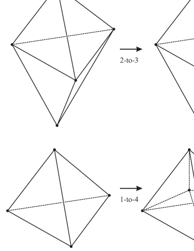
Figure 1: The $2$-to-$3$ and the $1$-to-$4$ moves on triangulations.

Remark 1.2.

Enumerating by computer the triangulations of closed orientable manifolds is in principle easy, even if computationally demanding. For increasing $n\geq 1$ one lists all the possible orientation-reversing pairings between the faces of $n$ tetrahedra yielding a connected result, and one checks that in the quotient space the link of every vertex is the $2$-sphere $S^{2}$ (to do which one only has to show that it has Euler characteristic $2$).

Here is a useful alternative viewpoint on triangulations. Let $M$ have one, and consider the $2$-skeleton of the cell subdivision dual to the triangulation, as suggested in Fig. 2-left.

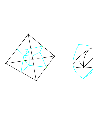
Figure 2: Duality between triangulations and spines.

This gives a spine of $M$ minus the vertices of the triangulation, namely a complex onto which this space collapses. This complex is actually a special polyhedron, namely one satisfying the following conditions:

• It consists of non-singular surface points as in Fig. 3-left, of singular points giving triple lines as in Fig. 3-center, and of at least one singular vertex as in Fig. 3-right;

• The connected components of the set of non-singular points are open discs.

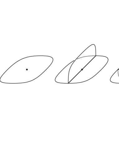
Figure 3: Special polyhedra.

The construction can be reversed: using a technical notion of orientability for a special polyhedron (see for instance [6]) one uses Fig. 2-right to associate to an orientable special polyhedron a set of tetrahedra and a pairing between their faces. As illustrated below, this does not always give a triangulation of a closed manifold, but one can check whether it does along the lines of Remark 1.2. The spine versions of the moves on triangulations are shown in Fig. 4.

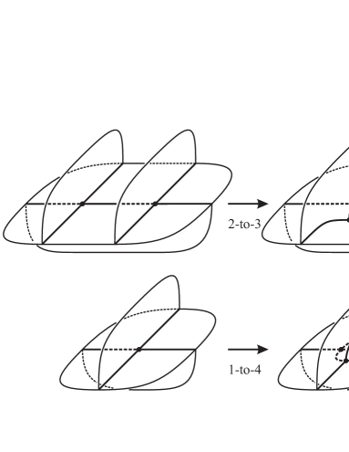
Figure 4: The $2$-to-$3$ and the $1$-to-$4$ moves on special spines.

Ideal triangulations

Turning to the case of a compact manifold $M$ with non-empty boundary $\partial M$, one can adapt to $M$ the notion of (loose) triangulation by calling ideal triangulation any of the following pairwise equivalent notions:

• A realization of $M$ minus its boundary as the space obtained by first gluing a finite number of disjoint tetrahedra along simplicial maps, and then removing the vertices;

• A realization of the space $X$ obtained from $M$ by collapsing each component of $\partial M$ to a point as the quotient of a disjoint union of tetrahedra under a simplicial pairing of the faces, in such a way that the quotient vertices correspond to the collapsed components of $\partial M$;

• A realization of $M$ as a gluing of truncated tetrahedra as in Fig. 5, with gluings between the lateral hexagons induced by simplicial gluings of the non-truncated tetrahedra.

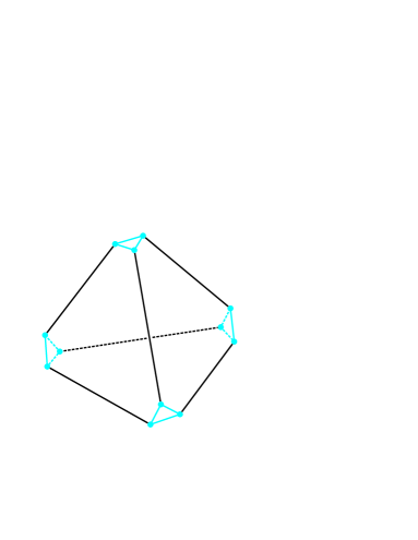
Figure 5: A truncated tetrahedron.

For the next result we refer again to [17]:

Theorem 1.3.

Any compact orientable $3$-manifold $M$ with non-empty boundary admits ideal triangulations, and any two of them consisting of at least two tetrahedra can be transformed into each other by repeated applications of the $2$-to-$3$ move shown in Fig. 1-top and its inverse.

Remark 1.4.

It is actually quite easy to deduce Theorem 1.1 from Theorem 1.3. One only needs to remark that removing some number $v$ of open $3$-balls from a connected and closed $M$ is a well-defined operation, from the result of which $M$ can be reconstructed unambiguously by capping off the boundary spheres. Moreover the $1$-to-$4$ move of Fig. 1-bottom is one that allows to increase by $1$ the number of vertices of an ideal triangulation, and hence to increase by $1$ the number of punctures in a punctured closed manifold represented by the triangulation.

The dual viewpoint of special spines carries over to the case of manifolds with boundary, and the corresponding statement is actually even more expressive:

Theorem 1.5.

• Each orientable compact $3$-manifold with non-empty boundary admits special spines;

• Each orientable special polyhedron is the spine of a unique $3$-manifold with non-empty boundary;

• Two special spines of the same $3$-manifold with non-empty boundary, both having at least two vertices, are related to each other by repeated applications of the $2$-to-$3$ move of Fig. 4-top and its inverse.

Remark 1.6.

We have repeatedly excluded from our statements the triangulations consisting of one tetrahedron only (and, dually, the spines having one vertex only). This is not a serious issue, because only a small number of uninteresting manifolds are described by these triangulations or spines.

Knots, links and graphs

Besides manifolds, knots are the next main objects of interest in $3$-dimensional topology. According to the basic definition, a knot is a tamely embedded circle in $3$-space, but one can easily extend the situation by considering links, defined as disjoint unions of knots, and let the ambient manifold in which a link is embedded be an arbitrary closed one. This leads to considering pairs $(M,L)$, with closed $M$ and $L\subset M$ a link, that we will always view up to equivalence of pairs (in the appropriate category) without further mention. We then define a triangulation of a link-pair $(M,L)$ as a (loose) triangulation of $M$ that contains $L$ as a subset of its $1$-skeleton. The next result was implicit in the work of Turaev and Viro [56] and was formally established by Amendola [2] (see also Pervova and the author [47] for more on spines of link-pairs):

Theorem 1.7.

Every link-pair $(M,L)$ with non-empty $L$ admits triangulations with precisely one vertex on each component of $L$. Any two such triangulations of $(M,L)$ consisting of at least two tetrahedra can be transformed into each other by repeated applications of the $2$-to-$3$ move shown in Fig. 1-top, and of the inverse of this move applied when the edge that disappears with the move does not belong to $L$.

A further category of objects that one deals with is given by the pairs $(M,G)$ where $M$ is a closed $3$-manifold and $G\subset M$ is a graph, that is a $1$-subcomplex of $M$. A triangulation of $(M,G)$ is one of $M$ that contains $G$ as a subcomplex of its $1$-skeleton. The previous result holds also for these objects, with the requirement that the triangulation should have one vertex at each vertex of $G$ and one on each knot component of $G$.

Orbifolds

We finally introduce orbifolds, defined as spaces having a singular differentiable structure locally defined as the quotient of Euclidean space under the action of a finite group of orientation-preserving diffeomorphisms. Since a finite orientable differentiable action is conjugate to a special orthogonal one, one sees that the local group acting can be assumed to be either cyclic, or dihedral, or the automorphism group of one of the Platonic solids. This implies that the support of a (closed, orientable, locally orientable) $3$-orbifold is a closed orientable $3$-manifold, in which the singular locus is a trivalent graph with edges labelled by integers and local aspect as in Fig. 6.

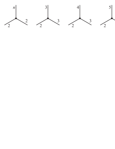
Figure 6: Local aspect of a closed locally orientable $3$-orbifold.

2 Hyperbolic structures

In this section we review the definition of hyperbolic $n$-space, we summarize its main features, and we define the hyperbolic structures we will be interested in constructing on each of the types of topological $3$-dimensional objects illustrated in the previous section.

Hyperbolic $n$-space

The $n$-dimensional hyperbolic space ${\mathbb{H}}^{n}$ can be defined as the only complete and simply connected Riemannian $n$-manifold having all sectional curvatures equal to $-1$, see [15]. For our purposes it will however be helpful to have at hand the following concrete models of this space:

• The disc model, defined as the open unit disc

  $$B^{n}=\{x\in{\mathbb{R}}^{n}:\ \|x\|<1\}$$

  endowed with the metric

  $$\,\mathrm{d}s^{2}_{x}=\frac{\,\mathrm{d}x^{2}}{4\left(1-\|x\|^{2}\right)^{2}};$$

• The half-space model, defined as the upper half-space

  $$\pi^{n}_{+}=\{x\in{\mathbb{R}}^{n}:\ x_{n}>0\}$$

  endowed with the metric

  $$\,\mathrm{d}s^{2}_{x}=\frac{\,\mathrm{d}x^{2}}{x_{n}^{2}};$$

• The hyperboloid model, defined as the hyperboloid

  $${\mathcal{H}}^{n}_{+}=\left\{x\in{\mathbb{R}}^{1,n}:\ \left\langle x|x\right\rangle_{(1,n)}=-1,\ x_{0}>0\right\},$$

  where ${\mathbb{R}}^{1,n}$ is the Minkowski space ${\mathbb{R}}^{n+1}$ endowed with the metric $\left\langle x|y\right\rangle_{(1,n)}=-x_{0}y_{0}+x_{1}y_{1}+\ldots+x_{n}y_{n}$; the Riemannian metric on ${\mathcal{H}}^{n}_{+}$ is given by the the restriction of the metric $\left\langle\cdot|\cdot\right\rangle_{(1,n)}$ to the hyperplanes tangent to ${\mathcal{H}}^{n}_{+}$, on which $\left\langle\cdot|\cdot\right\rangle_{(1,n)}$ is positive-definite.

The different models allow to single out some of the features of ${\mathbb{H}}^{n}$ that we will need below (see [54, 5, 51]):

• As one sees very well from the disc model, ${\mathbb{H}}^{n}$ has a natural compactification obtained by adding the points at infinity, that constitute an $(n-1)$-dimensional sphere $\partial{\mathbb{H}}^{n}$;

• The geodesics of ${\mathbb{H}}^{n}$ ending at the point $\infty$ in the half-space model $\pi_{n}^{+}$ are the vertical half-lines;

• A horosphere, defined as a connected complete hypersurface orthogonal to all the geodesics ending at a given point of $\partial{\mathbb{H}}^{n}$, called its center, if centered at $\infty$ in the $\pi^{n}_{+}$ model is given by a horizontal hyperplane, so it is endowed with a natural Euclidean structure; moreover the horosphere together with its center bound a topological disc in the compactified hyperbolic space, called a horoball;

• An isometry $\gamma$ of ${\mathbb{H}}^{n}$ must have fixed points either in ${\mathbb{H}}^{n}$ or in $\partial{\mathbb{H}}^{n}$, and hence it must be of one of the following types:

  • elliptic, namely with fixed points in ${\mathbb{H}}^{n}$; in this case, assuming $0$ is fixed in the disc model, $\gamma$ can be identified to an orthogonal matrix;

  • parabolic, namely with no fixed points in ${\mathbb{H}}^{n}$ and exactly one on $\partial{\mathbb{H}}^{n}$; in this case, assuming $\infty$ is fixed in the half-space model, $\gamma$ can be identified to an affine isometry of Euclidean space ${\mathbb{R}}^{n-1}$ acting horizontally on $\pi^{n}_{+}$; in particular, if $n=3$ and $\gamma$ preserves the orientation, it is just a horizontal translation;

  • hyperbolic, namely with no fixed points in ${\mathbb{H}}^{n}$ and exactly two on $\partial{\mathbb{H}}^{n}$; in this case, assuming $0$ and $\infty$ are fixed in $\pi^{n}_{+}$, it has the form

    $$\gamma(x)=\lambda\cdot\left(\begin{array}[]{cc}A&0\\ 0&1\end{array}\right)\cdot x$$

    with $A\in\mathrm{O}(n-1)$ and $\lambda>1$.

Closed and cusped hyperbolic manifolds

Let us temporarily drop our assumption that all manifolds should be compact, and take a possibly open $n$-dimensional one $N$. A hyperbolic structure on $N$ can be defined in one of the following equivalent ways:

• A complete Riemannian metric on $N$ with all sectional curvatures equal to $-1$;

• A complete Riemannian metric on $N$ making it locally isometric to ${\mathbb{H}}^{n}$;

• An identification between $N$ and the quotient of ${\mathbb{H}}^{n}$ under the action of a discrete and torsion-free group of isometries;

• A faithful representation of $\pi_{1}(N)$ into the group of the isometries of ${\mathbb{H}}^{n}$ having discrete and torsion-free image.

To state the first main general result we need to introduce further notation. Given a Riemannian manifold $N$ and $\varepsilon>0$, we define the $\varepsilon$-thick part $N_{[\varepsilon,+\infty)}$ of $N$ as the set of $x\in N$ such that every loop based at $x$ and having length at most $\varepsilon$ is null in $\pi_{1}(N,x)$, and the $\varepsilon$-thin part $N_{(0,\varepsilon]}$ of $N$ as the closure of the complement of its $\varepsilon$-thick part. The following holds true:

Theorem 2.1 (Margulis lemma).

There exists $\varepsilon>0$ depending only on $n$ such that if a hyperbolic $N$ is non-compact but has finite volume then its $\varepsilon$-thick part $N_{[\varepsilon,+\infty)}$ is compact, and its $\varepsilon$-thin part $N_{(0,\varepsilon]}$ is a disjoint union of components of the form $\Sigma\times[0,\infty)$, with $\Sigma$ a closed Euclidean $(n-1)$-manifold.

Since the only closed orientable surface carrying a Euclidean structure is the torus $T$, this result implies that an orientable $3$-dimensional finite-volume hyperbolic $N$ is the union of a compact manifold $M$ bounded by tori and a finite number of cusps based on tori, as suggested in Fig. 7.

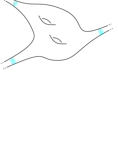
Figure 7: An allusive picture of a cusped hyperbolic $3$-manifold.

Moreover $N$ can be identified to the interior of $M$. For this reason, with a slight abuse of terminology, we will say that $M$ itself is hyperbolic, always meaning that the hyperbolic structure is actually defined on the interior of $M$, and that the toric boundary components of $M$ give rise to cusps.

The next general result is the following one:

Theorem 2.2 (Mostow rigidity).

If $n\geq 3$ two finite-volume hyperbolic $n$-manifolds having isomorphic fundamental groups are isometric to each other. In particular, every $n$-manifold carries at most one finite-volume hyperbolic metric up to isometry.

This deep theorem has the important consequence that any geometric invariant of a hyperbolic manifold, such as the volume or the length of the shortest geodesic for a closed one, is automatically a topological invariant. To state the next result, we need to recall that performing a Dehn filling of a torus boundary component $T$ of a compact $3$-manifold $M$ consists in gluing to $M$ the solid torus $D^{2}\times S^{1}$ along a homeomorphism $\partial(D^{2}\times S^{1})\to T$. The result of this operation depends only on the slope on $T$ that becomes contractible in the attached $D^{2}\times S^{1}$, namely on the isotopy class on $T$ of the simple non-trivial curve $f(S^{1}\times\{*\})$. If $M$ has several boundary component we will call Dehn filling of $M$ any manifold obtained by performing this operation on some (possibly all) of the toric components of $\partial M$. The next general result shows that in dimension three, given a cusped hyperbolic manifold, one can produce a wealth of new ones:

Theorem 2.3 (Thurston’s hyperbolic Dehn filling).

Let $M$ be a finite-volume hyperbolic $3$-manifold with cusps based on tori $T_{1},\ldots,T_{k}$. Then for $j=1,\ldots,k$ there exists a set finite $E_{j}$ of slopes on $T_{j}$ such that every Dehn filling of $M$ performed along slopes $\alpha_{1},\ldots,\alpha_{k}$ with $\alpha_{j}\not\in E_{j}$ is hyperbolic.

Note that the theorem includes the case of the “empty” filling of some cusp (or several ones), that leaves the cusp as is. We also remark in passing that one can define a natural topology on the space of hyperbolic manifolds and that taking a sequence of fillings of $M$ in which on each cusp the length of the slope (defined for instance as the norm of its coordinates with respect to some fixed homological basis) tends to infinity, one gets a sequence of hyperbolic manifolds converging to $M$, with volumes converging from below to that of $M$.

Hyperbolic manifolds with geodesic boundary

When a compact $3$-manifold $M$ has boundary components which are not tori, one has no hope to construct on it or on its interior a finite-volume hyperbolic structure (an infinite-volume non-rigid one often exists, but this is a completely different story). In this case one allows the boundary of $M$ to be part of the hyperbolic structure, in the form of a totally geodesic surface. To explain the matter in detail, we again temporarily remove the restriction that manifolds should be compact, and consider an arbitrary one $N$, possibly non-compact and with boundary, with the boundary itself possibly non-compact. We then say that $N$ is hyperbolic with geodesic boundary if it has a complete finite-volume Riemannian structure locally modeled on open subsets of a half-space in hyperbolic space ${\mathbb{H}}^{3}$. Mirroring $N$ in its boundary we get the double $D(N)$ of $N$, which is hyperbolic without boundary, so its universal cover can be identified to ${\mathbb{H}}^{3}$. Moreover $\partial N$ is a totally geodesic surface in $D(N)$, and the universal cover of $N$ can be identified to the closure of any connected component in ${\mathbb{H}}^{3}$ of the complement of the family of disjoint planes in ${\mathbb{H}}^{3}$ that project in $D(N)$ onto $\partial N$. This allows the following alternative description of a hyperbolic structure with geodesic boundary:

• A hyperbolic structure with geodesic boundary on $N$ corresponds to a realization of $N$ as the quotient of the intersection $H$ of a family of half-spaces in ${\mathbb{H}}^{3}$ under the action of a discrete and torsion-free group of isometries of ${\mathbb{H}}^{3}$ that leave $H$ invariant.

Let us now describe the thin part of a finite-volume hyperbolic $3$-manifold $N$ with geodesic boundary. Since $D(N)$ is finite-volume hyperbolic without boundary, for $\varepsilon$ less than the third Margulis constant the $\varepsilon$-thin part of $D(N)$ consists of cusps based on tori. Each such cusp is either disjoint from $\partial N$, in which case it gives rise to a toric cusp in $N$, or it is cut into two symmetric pieces by $\partial N$. It is then not too difficult to see that the corresponding portion of the thin part of $N$ is an annular cusp, namely of type $A\times[0,+\infty)$, with $A$ a Euclidean annulus obtained by gluing together two opposite sides of a rectangle.

This discussion implies that a finite-volume hyperbolic $3$-manifold $N$ with geodesic boundary compactifies to a certain $M$ with a specified family of closed annuli ${\mathcal{A}}$ on $\partial M$, so that $N$ is given by $M$ minus ${\mathcal{A}}$ and the toric components of $\partial M$. Note that $\partial M$ cannot contain spheres and no annulus in ${\mathcal{A}}$ can lie on a toric component of $\partial M$.

In the sequel we will sometimes speak with a slight abuse of a hyperbolic compact $(M,{\mathcal{A}})$ to mean that a (complete and finite-volume, as always) hyperbolic metric is defined on $M$ minus the union of ${\mathcal{A}}$ and all the toric boundary components of $\partial M$.

Hyperbolic structures with geodesic boundary still enjoy Mostow rigidity, but only in the sense that each manifold can carry at most one such structure up to isometry: it is not true in this context that the fundamental group determines the structure, as shown by Frigerio [18].

Links, orbifolds, and graphs

For a link-pair $(M,L)$ with closed $M$ a hyperbolic structure is simply one on the exterior of $L$ in $M$, with one cusp for each component of $L$.

Turning to a $3$-orbifold, recall that the finite local action on ${\mathbb{R}}^{3}$ defining it can be assumed to be orthogonal, up to conjugation, and that the stabilizer of a point in the group of isometries of hyperbolic space is the orthogonal group. The notion of a hyperbolic structure on a closed $3$-orbifold is then an obvious extension of those already defined: it is a complete finite-volume singular Riemannian metric locally given by the quotient of an open ball in ${\mathbb{H}}^{3}$ under a finite action of isometries fixing the center of the ball. Versions of the definition for orbifolds with cusps and/or with boundary exist but will not be referred to below.

For a graph-pair $(M,G)$ we will consider three different types of hyperbolic structure:

• With totally geodesic boundary: an ordinary hyperbolic structure on the exterior $X$ of $G$ in $M$; note that the knot components of $G$ give rise to toric cusps, whereas components with vertices give compact components of the boundary;

• Of orbifold type: an orbifold hyperbolic structure on $M$ with some admissible labelling of the edges of $G$ by integers;

• With parabolic meridians: a hyperbolic structure on $(X,{\mathcal{A}})$, where $X$ is the exterior of $G$ in $M$ and ${\mathcal{A}}$ is a system of meridinal annuli of the edges of $G$; note that for such a structure there is one toric cusp for each component of $G$, one annular cusp for each edge joining two vertices (or a vertex to itself), and one thrice punctured sphere of geodesic boundary for each vertex of $G$.

Hyperbolisation

So far we have not explain for what reason one should hope a $3$-dimensional manifold (or graph, or orbifold) to have a hyperbolic structure. We now discuss the obstructions to the existence of such a structure and state the extremely deep results according to which the absence of these obstructions is actually sufficient to guarantee hyperbolicity. To begin, we recall that an essential surface in a $3$-manifold $M$ is a properly embedded one whose fundamental group, under the inclusion, injects into that of $M$, and which is not parallel to the boundary. It is not too difficult to show that a hyperbolic manifold cannot contain essential surfaces with non-negative Euler characteristic (that is, spheres, tori, discs, or annuli). The following result has first been proved by Thurston [55] for Haken manifolds (those containing some essential surface), remained as a conjecture for a long time, and was eventually established by Perelman [44, 45, 46] (see also [7]):

Theorem 2.4.

If a compact $3$-manifold $M$ with (possibly empty) boundary consisting of tori does not contain any essential surface with non-negative Euler characteristic then $M$ is either hyperbolic or a Dehn filling of $P\times S^{1}$, where $P$ is the $2$-sphere minus three open discs.

(The reason why Dehn fillings of $P\times S^{1}$ make an exception is that they are the only manifolds containing a $\pi_{1}$-injective immersed torus but no embedded essential one, thanks to a result of Casson and Jungreis [13].)

The philosophy underlying the previous theorem is that cutting a manifold along a surface with non-negative Euler characteristic one gets a (possibly disconnected) simpler one, from which the original manifold can be reconstructed. Therefore hyperbolic manifolds and Dehn fillings of $P\times S^{1}$ can be viewed as building blocks for general $3$-manifolds.

Hyperbolization holds true, with the necessary adjustments, for manifolds with more general boundary (and annuli on this boundary), see [21], and for orbifolds (which requires in particular the introduction of the notion of essential $2$-suborbifold), see [8, 14].

An important consequence of the hyperbolization theorem is that if a graph-pair $(M,G)$ admits a hyperbolic structure with totally geodesic boundary on its exterior then for any admissible labelling of the edges, which turns $(M,G)$ into an orbifold, $(M,G)$ admits a corresponding orbifold hyperbolic structure, and that if for some labelling of the edges $(M,G)$ admits an orbifold hyperbolic structure then it admits one with parabolic meridians.

3 Cusped manifolds

We will now describe the algorithmic approach to the construction and recognition of cusped hyperbolic manifolds, carried out with extreme success by Callahan, Hildebrandt and Weeks [11].

Hyperbolic ideal tetrahedra

Let us start from a compact $3$-manifold $M$ with non-empty boundary consisting of tori, and from an ideal triangulation ${\mathcal{T}}$ of $M$. The idea to hyperbolize $M$, which dates back to Thurston [54], is to choose a hyperbolic shape separately for each tetrahedron in ${\mathcal{T}}$ and then to ensure consistency and completeness of the structure induced on $M$. To spell out this idea we begin by defining a hyperbolic ideal tetrahedron as the convex envelope $\Delta$ in ${\mathbb{H}}^{3}$ of four non-aligned points in $\partial{\mathbb{H}}^{3}$, endowed with the orientation induced by ${\mathbb{H}}^{3}$. (Recall that three points on $\partial{\mathbb{H}}^{3}={\mathbb{P}}^{1}({\mathbb{C}})$ are always aligned, namely there exists a geodesic plane having all three of them as points at infinity.) Intersecting $\Delta$ with a small enough horosphere centered at any of its vertices, one gets a Euclidean triangle, which gets rescaled if the horosphere is shrunk. Moreover one can see that two triangles lying on horospheres centered at distinct vertices have the same angle at the edge of $\Delta$ joining these vertices, which implies that the four triangles at the vertices of $\Delta$ are actually similar to each other, so $\Delta$ determines a similarity class of an oriented triangle in the plane, and the converse is also true.

To be more specific, let us note that the oriented isometries of ${\mathbb{H}}^{3}$ act in a triply transitive way on $\partial{\mathbb{H}}^{3}$, so without loss of generality we can assume in the half-space model $\pi^{3}_{+}$ viewed as $(0,+\infty)\times{\mathbb{C}}$, that a positively oriented triple of vertices of $\Delta$ is $(0,1,\infty)$. This implies that the fourth vertex is some $z\in{\mathbb{C}}$ with $\Im(z)>0$, namely $z\in\pi^{2}_{+}$. Then the hyperbolic structure of $\Delta$ is determined by $z$, that we will call module of $\Delta$ along the edge $(0,\infty)$, see Fig. 8.

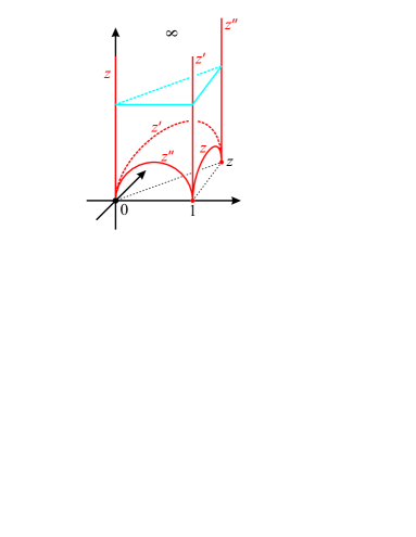
Figure 8: Modules of a hyperbolic ideal tetrehedron.

Moreover the modules of $\Delta$ along the other edges are as shown in the figure, with $z^{\prime}=\frac{1}{1-z}$ and $z^{\prime\prime}=1-\frac{1}{z}$. In particular, $\Delta$ has the same module along any two edges opposite to each other. And, converseley, once an orientation and a pair of opposite edges have been fixed on an abstract tetrahedron, the choice of any $z\in\pi^{2}_{+}$ turns the tetrahedron into an ideal hyperbolic one as in Fig. 8.

Consistency and completeness

Let us return to our $M$ ideally triangulated by ${\mathcal{T}}$, and assume that there are $n$ tetrahedra $\Delta_{1},\ldots,\Delta_{n}$ and $k$ toric boundary components $T_{1},\ldots,T_{k}$. Choosing a hyperbolic structure on $\Delta_{1},\ldots,\Delta_{n}$ corresponds to choosing $z_{1},\ldots,z_{n}\in\pi^{2}_{+}$, that we can view as variables. Using again the fact that the isometries of ${\mathbb{H}}^{3}$ act in a triply transitive way on $\partial{\mathbb{H}}^{3}$, it is now easy to see that for any choice of $z_{1},\ldots,z_{n}$ the hyperbolic structure on the tetrahedra extends to the interior of the glued faces in $M$. We then have the following:

Proposition 3.1 (Consistency equations).

The hyperbolic structure defined by $z_{1},\ldots,z_{n}$ extends along an edge $e$ of ${\mathcal{T}}$ in $M$ if and only if the product of all the modules of $\Delta_{1},\ldots,\Delta_{n}$ (counted with multiplicity if $e$ is multiply adjacent to some $\Delta_{j}$) equals $1$, and the sum of the arguments of these modules equals $2\pi$.

Remark 3.2.

If the product of the modules along an edge equals $1$, then the sum of the arguments of these modules is a positive multiple of $2\pi$. Using this fact and the observation that $\chi(M)=0$, because $\partial M$ consists of tori, one then sees that if the products of the modules along all edges of ${\mathcal{T}}$ equals $1$, then the sum of the arguments always equals $2\pi$. This implies that consistency of the hyperbolic structure defined by $z_{1},\ldots,z_{n}$ translates into $n$ algebraic equations. (See also below for the number of these equations.)

Suppose now that $z_{1},\ldots,z_{n}$ satisfy the consistency equations along all the edges of ${\mathcal{T}}$. Then each boundary torus $T_{j}$ is obtained by gluing Euclidean triangles along similarities, and consistency ensures that the similarity structure on the triangles extends to the edges and the vertices. Summing up, $z_{1},\ldots,z_{n}$ induce a similarity structure on each $T_{j}$, and we have:

Proposition 3.3.

The hyperbolic structure on $M$ defined by $z_{1},\ldots,z_{n}$ is complete if and only if the induced similarity structure on each $T_{j}$ is actually Euclidean.

To turn the completeness condition into equations, we note that a similarity structure on a torus $T$ induces a representation (the holonomy) of $\pi_{1}(T)$ into the group of complex-affine automorphisms of ${\mathbb{C}}$. This representation is well-defined up to conjugation, so its dilation component $\rho:\pi_{1}(T)\to{\mathbb{C}}_{*}$ is well-defined, and of course $T$ is Euclidean if and only if $\rho$ is identically $1$. If the similarity structure on $T$ is obtained by gluing triangles with specified modules, and $\alpha$ is a simplicial loop in the resulting triangulation, one can easily show that $\rho(\alpha)$ is the product of the modules of the triangles that $\alpha$ leaves to its left, as suggested in Fig. 9. Therefore:

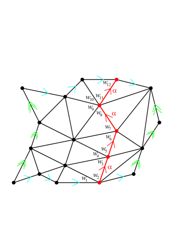
$\Rightarrow\ \rho(\alpha)=w_{1}\cdots w_{12}$

Figure 9: Computation of the dilation component of the holonomy of a simplicial loop.

Proposition 3.4 (Completeness equations).

For $j=1,\ldots,k$ let $\lambda_{j}$ and $\mu_{j}$ be generators of $\pi_{1}(T_{j})$. The hyperbolic structure on $M$ defined by $z_{1},\ldots,z_{n}$ is complete if and only if for all $j$ the product of the modules of the triangles on $T_{j}$ that $\lambda_{j}$ leaves to its left equals $1$, and the same happens for $\mu_{j}$.

Remark 3.5.

The images of $\lambda_{j}$ and $\mu_{j}$ under the holonomy representation of $\pi_{1}(T)$ associated to a similarity structure are commuting complex-affine automorphisms of ${\mathbb{C}}$. The condition $\rho(\lambda_{j})=1$ means that the holonomy of $\lambda_{j}$ is a translation; if this translation is non-trivial then also $\mu_{j}$ maps to a translation, therefore $\rho(\mu_{j})=1$. This shows that the two conditions to impose on each $T_{j}$ are “almost” equivalent to each other, so in practice one adds to the $n$ consistency equations only $k$, and not $2k$, completeness equations. Moreover it was shown by Neumann and Zagier [43] that if a solution exists then $k$ of the consistency equations can be dismissed; moreover the complete structure corresponds to a smooth point in the space of deformations of the structure, which is a $k$-dimensional algebraic variety. This fact can be exploited for instance to establish Theorem 2.3.

To conclude the discussion on the construction of the hyperbolic structure on a would-be cusped manifold $M$, we note that using an arbitrary ideal triangulation ${\mathcal{T}}$ of $M$ it is not true that a solution of the corresponding consistency and completeness equations always exists, even if $M$ is actually hyperbolic. And, as a matter of fact, it is not even known that one ${\mathcal{T}}$ such that the corresponding equations have a genuine solution exists (despite the wrong statement in [5] that this follows from [16], see also below). However when one starts from a minimal triangulation of a hyperbolic $M$, namely one with a minimal number of tetrahedra, the solution always exists in practice. Weeks’ wonderful software SnapPea [61] is capable (among other things) to find a minimal triangulation of a given (a priori possibly non-hyperbolic) $M$, to seek for a solution of the corresponding equations, and also to deduce from patterns it sees in the triangulation the existence of topological obstructions to hyperbolicity. It is using these features (and the recognition machinery described in the rest of this section) that the census [11] of cusped manifolds triangulated by at most $7$ tetrahedra has been obtained.

Canonical decomposition

Once the hyperbolic structure on a cusped $M$ has been constructed, the need naturally arises to recognize such an $M$, namely to be able to effectively determine whether $M$ is the same as any other given cusped manifold. Several hyperbolic invariants, and chiefly the volume (which is easily computed from a hyperbolic ideal triangulation by means of the Lobachevski function, see [42]), can often distinguish manifolds, but different manifolds actually can have the same volume, as proved by Adams [1], and other invariants, so the need of a complete one remains. This complete invariant is provided by a result of Epstein and Penner [16], and it allows to perform the recognition very efficiently. We will first state this result informally and then provide the necessary details.

The basic underlying idea is best described starting from an arbitrary compact Riemannian manifold $X$ (of any dimension) with non-empty boundary. In this case one can define the cut-locus $\textrm{Cut}_{X}(\partial X)$ of $\partial X$ in $X$ as the set of points joined by more than one distance-minimizing path to $\partial X$. To visualize $\textrm{Cut}_{X}(\partial X)$, imagine that we start pushing all the components of $\partial X$ towards the interior of $X$, all at the same pace. At some point some collision (or self-collision) will start occurring; we then fuse together the collided points, leave them still henceforth, and keep pushing the rest. Eventually we exhaust all the space available in $M$ and we are left with $\textrm{Cut}_{X}(\partial X)$ in the form of the membrane on which the collisions have taken place. (See Fig. 10

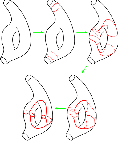
Figure 10: The cut locus of the boundary in a Riemannian surface as the result of pushing the boundary towards the interior as far as possible.

for an allusive picture in dimension $2$.) This description should make it obvious that $\textrm{Cut}_{X}(\partial X)$ is a compact subset of $X$ onto which $X$ retracts, and that it has dimension at least one less than $X$. Supposing $X$ has dimension $3$ one can in addition imagine that in a generic situation $\textrm{Cut}_{X}(\partial X)$ will be a special spine of $X$, and therefore that dual to it there will be a topological ideal triangulation of $X$. In more general contexts dual to $\textrm{Cut}_{X}(\partial X)$ there will be a decomposition of $X$ into ideal polyhedra more complicated than tetrahedra.

Turning to a cusped hyperbolic $M$, we first note that we cannot take $\textrm{Cut}_{M}(\partial M)$, because $\partial M$ is at infinite distance from any point in the interior of $M$, since $\partial M$ is not really part of the hyperbolic structure, but rather of its compactification. Recall however that each cusp of $M$ has the form $T\times[0,\infty)$, where $T$ is a flat torus, and more precisely the image in $M$ of a horoball of ${\mathbb{H}}^{3}$ acted on by the ${\mathbb{Z}}\oplus{\mathbb{Z}}$ lattice of the parabolic elements of $\pi_{1}(M)$ fixing the center of the horoball. If we replace the cusp $T\times[0,+\infty)$ with $T\times[h,+\infty)$ for some $h>0$ we get a smaller cusp, with volume that tends to $0$ as $h\to+\infty$. Therefore for sufficiently small $v>0$ we can take disjoint cusps at each end of $M$ all having volume $v$, and call $M^{(v)}$ the complement in $M$ of their interior. The following fact has an intimately hyperbolic nature, as we will explain before providing a detailed proof:

Proposition 3.6.

$\textrm{Cut}_{M^{(v)}}(\partial M^{(v)})$ is independent of $v$.

To appreciate this result, consider the case of a Riemannian manifold $X=T\times[0,1]$, with metric $\,\mathrm{d}s^{2}_{(p,t)}=f(t)\cdot\,\mathrm{d}\sigma^{2}_{p}+\,\mathrm{d}t^{2}$, where $\,\mathrm{d}\sigma^{2}$ is a flat metric on $T$ giving it area $1$, and $f$ is a smooth incresasing function such that $f(t)=1$ for $0\leq t\leq\frac{1}{3}$ and $f(t)=2$ for $\frac{5}{6}\leq t\leq 1$. Viewing $T\times\left[0,\frac{1}{3}\right]$ and $T\times\left[\frac{5}{6},1\right]$ as the ends of $X$, we see that they both have volume $\frac{1}{3}$, so $X^{\left(\frac{1}{3}\right)}=T\times\left[\frac{1}{3},\frac{5}{6}\right]$, and $\textrm{Cut}_{X^{\left(\frac{1}{3}\right)}}\left(\partial X^{\left(\frac{1}{3}\right)}\right)=T\times\{\frac{7}{12}\}$. However $X^{\left(\frac{1}{6}\right)}=T\times\left[\frac{1}{6},\frac{11}{12}\right]$ and $\textrm{Cut}_{X^{\left(\frac{1}{6}\right)}}\left(\partial X^{\left(\frac{1}{6}\right)}\right)=T\times\{\frac{13}{24}\}$.

Proof of Proposition 3.6. Assume two cusps of volume $v$ in $M$ get lifted in ${\mathbb{H}}^{3}$ to horoballs centered at $\infty$ and at $0$ in the $\pi^{3}_{+}$ model of ${\mathbb{H}}^{3}$, namely to some half-space $O_{1}=[h_{1},+\infty)\times{\mathbb{R}}^{2}$ and to some Euclidean ball $O_{2}$ of radius $\frac{h_{2}}{2}$ centered at $(0,0,\frac{h_{2}}{2})$, so that its top point has height $h_{2}$. Since the cusps in $M$ are disjoint or coincide, one has $h_{2}<h_{1}$. Now suppose that the action of the ${\mathbb{Z}}\oplus{\mathbb{Z}}$ lattice of parabolic elements of $\pi_{1}(M)$ fixing $\infty$ gives as a quotient of $\{0\}\times{\mathbb{R}}^{2}$ a flat torus of area $a_{1}$. Note that $a_{1}$ is independent of $v$, namely, if we change $v$ then the height $h_{1}$ changes but the area $a_{1}$ does not. Moreover $v$ is equal to the integral of the volume form $\frac{1}{x_{3}^{3}}\,\mathrm{d}x_{1}\,\mathrm{d}x_{2}\,\mathrm{d}x_{3}$ of ${\mathbb{H}}^{3}$ over $[h_{1},+\infty)\times A_{1}$, where $A_{1}$ is a parallelogram of area $a_{1}$, therefore $v=\frac{a_{1}}{2h_{1}^{2}}$. Applying the inversion with respect to the radius-1 sphere centered at $0$, which is a hyperbolic isometry, $O_{2}$ becomes the half-plane $\left[\frac{1}{h_{2}},+\infty\right)\times{\mathbb{R}}^{2}$, and the computation already performed shows that $v=\frac{a_{2}h_{2}^{2}}{2}$, for some $a_{2}$ again independent of $v$. The surface of the points having equal distance from $O_{1}$ and from $O_{2}$ is of course determined by the point in which it intersects the $x_{3}$-axis, whose height $h$ must satisfy

$$\int_{h_{2}}^{h}\frac{\,\mathrm{d}x_{3}}{x_{3}}=\int_{h}^{h_{1}}\frac{\,\mathrm{d}x_{3}}{x_{3}}\ \Rightarrow\ \log(h)-\log(h_{2})=\log(h_{1})-\log(h)$$

$$\ \Rightarrow\ 2\log(h)=\log(h_{1}h_{2})\ \Rightarrow\ h=\sqrt{h_{1}h_{2}}.$$

The relations $v=\frac{a_{1}}{2h_{1}^{2}}$ and $v=\frac{a_{2}h_{2}^{2}}{2}$ established above now easily imply that $\sqrt{h_{1}h_{2}}=\frac{a_{1}}{a_{2}}$ is indeed independent of $v$, and the conclusion follows. $\square$

We can now state the result of [16]:

Theorem 3.7 (Epstein-Penner canonical decomposition).

If $M$ is a cusped hyperbolic $3$-manifold then dual to $\textrm{Cut}_{M^{(v)}}(\partial M^{(v)})$ there is a decomposition of $M$ into hyperbolic ideal polyhedra whose combinatorics and hyperbolic shape of the blocks depends on $M$ only.

Once the Epstein-Penner canonical decompositions of two given cusped hyperbolic manifolds have been determined, to compare the manifolds for equality one then only needs to compare the canonical decompositions for combinatorial equivalence. Note that one does not need to check that the hyperbolic shapes of the polyhedra are the same, since combinatorial equivalence of the decompositions already ensures that the manifolds are homeomorphic to each other (whence, by rigidity, isometric to each other).

The light-cone and the convex hull construction

To show how one can actually construct the Epstein-Penner canonical decomposition of a given ideally triangulated cusped manifold, we will exploit more of the hyperboloid model ${\mathcal{H}}^{n}_{+}$ of ${\mathbb{H}}^{n}$ than we have done so far. We first define the (future) light-cone in the Minkoswki space ${\mathbb{R}}^{1,n}$ with scalar product $\left\langle\cdot|\cdot\right\rangle_{(1,n)}$ as

$${\mathcal{L}}^{n}_{+}=\left\{y\in{\mathbb{R}}^{1,n}:\ \left\langle y|y\right\rangle_{(1,n)}=0,\ y_{0}>0\right\}$$

and we remark that there is a natural identification between $\partial{\mathbb{H}}^{n}$ and the projectivized light-cone ${\mathbb{P}}\left({\mathcal{L}}^{n}_{+}\right)$. Moreover for all $y\in{\mathcal{L}}^{n}_{+}$ one can define as follows an associated horoball

$$B_{y}=\left\{x\in{\mathcal{H}}^{n}_{+}:\ \left\langle x|y\right\rangle_{(1,n)}\geq-1\right\}$$

and its boundary horosphere $H_{y}=\partial B_{y}$. It is not hard to see that $B_{y}$ is centered at $[y]\in{\mathbb{P}}\left({\mathcal{L}}^{n}_{+}\right)=\partial{\mathbb{H}}^{n}$, and that all horoballs centered at some $p\in{\mathbb{P}}\left({\mathcal{L}}^{n}_{+}\right)=\partial{\mathbb{H}}^{n}$ have the form $B_{y}$ for some $y\in{\mathcal{L}}^{n}_{+}$ with $[y]=p$. Note that $B_{y^{\prime}}\subset B_{y}$ if $y^{\prime}=\lambda y$ with $\lambda>1$.

Turning to the effective construction of the Epstein-Penner decomposition, let us fix a cusped hyperbolic $3$-manifold $M$, and a set of disjoint cusps in $M$ all having one and the same volume $v$. These cusps lift in the universal cover of $M$, that we identify with ${\mathcal{H}}^{3}_{+}$, to a family of disjoint horoballs $\{B_{y}:\ y\in{\mathcal{P}}\}$ for some ${\mathcal{P}}\subset{\mathcal{L}}^{3}_{+}$. Let us now establish the following crucial property of ${\mathcal{P}}$:

Lemma 3.8.

${\mathcal{P}}$ is discrete.

Proof.

It is of course sufficient to show that for all $h>0$ the set $\{p\in{\mathcal{P}}:\ x_{0}(p)\leq h\}$ is finite. Assuming the contrary and projecting to the disc model $B^{3}$, we would get an infinite family of horoballs that, as Euclidean balls, have radius bounded from below. But this is impossible since the horoballs must be disjoint from each other. ∎

We now define $C$ as the convex hull of ${\mathcal{P}}$ in ${\mathbb{R}}^{1,3}$, and we note that ${\mathcal{P}}$, and hence $C$, are invariant under the action of $\pi_{1}(M)$, which extends from ${\mathcal{H}}^{3}_{+}$ to ${\mathbb{R}}^{1,3}$. The following is established in [16]:

Proposition 3.9.

• $C\cap{\mathcal{L}}^{3}_{+}=\{\lambda\cdot p:\ p\in{\mathcal{P}},\ \lambda\geq 1\}$;

• For all $x\in{\mathcal{H}}^{3}_{+}$ the half-line $\{t\cdot x:\ t\geq 0\}$ intersects $C$ in a half-line $\{t\cdot x:\ t\geq\lambda_{0}(x)\}$ for a suitable $\lambda_{0}(x)$, and $\lambda_{0}(x)\cdot x\in\partial C$:

• $\partial C\setminus{\mathcal{L}}^{3}_{+}$ consists precisely of the points $\lambda_{0}(x)\cdot x$ for $x\in{\mathcal{H}}^{3}_{+}$, therefore the radial projection is a bijection between $\partial C\setminus{\mathcal{L}}^{3}_{+}$ and ${\mathcal{H}}^{3}_{+}$;

• $\partial C$ consists of a $\pi_{1}(M)$-invariant family of finite-faced polyhedra that intersect ${\mathcal{L}}^{3}_{+}$ precisely at their vertices;

• The polyhedra of which $\partial C$ consists, projected first radially to ${\mathcal{H}}^{3}_{+}$ and then to $M$ under the action of $\pi_{1}(M)$, give the ideal decomposition of $M$ dual to $\textrm{Cut}_{M^{(v)}}(\partial M^{(v)})$ as in Theorem 3.7

The tilt formula

Let us suppose that $M$ is a cusped hyperbolic manifold with a given hyperbolic ideal triangulation ${\mathcal{T}}$. We will now describe a method, based on the results of Sakuma and Weeks [60, 53] and exploited by Weeks’ software SnapPea [61], to decide whether the Epstein-Penner canonical decomposition of $M$ is actually ${\mathcal{T}}$ or can be obtained from ${\mathcal{T}}$ by merging together some of the tetrahedra into more complicated polyhedra. To this end we fix some $v>0$ such that $M$ contains disjoint cusps of volume $v$ at all its ends (and note that $v$ is easy to find using the combinatorics of ${\mathcal{T}}$ and the geometry of the hyperbolic tetrahedra that ${\mathcal{T}}$ consists of). We then concentrate on a $2$-face $F$ of ${\mathcal{T}}$, to which two tetrahedra $\Delta_{1}$ and $\Delta_{2}$ will be incident. Let us lift $F,\Delta_{1},\Delta_{2}$ in ${\mathcal{H}}^{3}_{+}$ to an ideal triangle $\widetilde{F}$ and two ideal tetrahedra $\widetilde{\Delta}_{1}$ and $\widetilde{\Delta}_{2}$ such that $\widetilde{F}=\widetilde{\Delta}_{1}\cap\widetilde{\Delta}_{2}$. The choice of $v$ allows us to associate a point on the light-cone ${\mathcal{L}}^{3}_{+}$ to each ideal vertex of $\widetilde{F},\widetilde{\Delta}_{1},\widetilde{\Delta}_{2}$, and we can consider the straight triangle $F^{\prime}$ and tetrahedra $\Delta^{\prime}_{1},\Delta^{\prime}_{2}$ in ${\mathbb{R}}^{1,3}$ having these points on ${\mathcal{L}}^{3}_{+}$ as vertices . Finally, we define $\vartheta(F)$ as the dihedral angle in ${\mathbb{R}}^{1,3}$ not containing $0$ formed along the plane containing $F^{\prime}$ by the half-hyperplanes containing $\Delta^{\prime}_{1}$ and $\Delta^{\prime}_{2}$, and we note that $\vartheta(F)$ is independent of the particular liftings chosen. The following is a direct consequence of Proposition 3.9:

Proposition 3.10.

${\mathcal{T}}$ is the Epstein-Penner decomposition of $M$ if and only if $\vartheta(F)<\pi$ for all $2$-faces $F$ of ${\mathcal{T}}$. More generally, the Epstein-Penner decomposition of $M$ is obtained from ${\mathcal{T}}$ by merging together some of the tetrahedra of ${\mathcal{T}}$ if and only if $\vartheta(F)\leq\pi$ for all $2$-faces $F$ of ${\mathcal{T}}$, and in this case the mergings to perform are those along the $F$’s such that $\vartheta(F)=\pi$.

When ${\mathcal{T}}$ does not meet the conditions of this proposition, namely when it contains some offending $2$-face $F$ with $\vartheta(F)>\pi$, a new triangulation ${\mathcal{T}}^{\prime}$ with better chances of being a subdivision of the Epstein-Penner decomposition is obtained by performing the 2-to-3 move along $F$. Note however that the move can be applied only if the two tetrahedra of ${\mathcal{T}}$ incident to $F$ are distinct. One can then start a process that searches for faces $F$ with $\vartheta(F)>\pi$ to which the $2$-to-$3$ move can be applied, applies the move and starts over again. The process can get stuck if all $F$’s with $\vartheta(F)>\pi$ are incident to the same tetrahedron on both sides, but it is shown in [53] that if the process does not get stuck then it converges in finite time to a subdivision of the Epstein-Penner decomposition. As a matter of fact, experimentally the process always converges, and it does so very quickly.

There is however one aspect of the process just described that we have not yet described how to perform algorithmically, namely the computation of the angle $\vartheta(F)$. This is done using the Sakuma-Weeks tilt formula, that constitutes the core of [53]. This formula associates a real number $t(\Delta,E)$, called the tilt, to each triangle $E$ in ${\mathbb{R}}^{1,3}$ with vertices on ${\mathcal{L}}^{3}_{+}$ and to each tetrahedron $\Delta$ with vertices on ${\mathcal{L}}^{3}_{+}$ having the triangle as a face. To do so, the following vectors are needed:

• The unit normal $p$ to $\Delta$, satisfying $\left\langle p|x\right\rangle_{(1,3)}=-1$ for all $x\in\Delta$;

• The outer unit normal $m$ to $E$, satisfying $\left\langle m|m\right\rangle_{(1,3)}=1$, $\left\langle m|x\right\rangle_{(1,3)}=0$ for all $x\in E$, and $\left\langle m|v\right\rangle_{(1,3)}<0$, where $v$ is the vertex of $\Delta$ opposite to $E$.

Then $t(\Delta,E)=\left\langle p|m\right\rangle_{(1,3)}$, and the knowledge of the tilts allows to apply Proposition 3.10 by means of the following:

Proposition 3.11.

With the notation introduced before Proposition 3.10, $\vartheta(F)<\pi$ if and only if $t(\Delta_{1}^{\prime},F^{\prime})+t(\Delta_{2}^{\prime},F^{\prime})<0$, and $\vartheta(F)=\pi$ if and only if $t(\Delta_{1}^{\prime},F^{\prime})+t(\Delta_{2}^{\prime},F^{\prime})=0$.

Rather than provinding a complete proof of this result, we motivate it using an example in one dimension less. We suppose in ${\mathbb{R}}^{1,2}$ that $F^{\prime}$ has vertices $\left(\begin{array}[]{c}1\\ 1\\ 0\end{array}\right)$ and $\left(\begin{array}[]{c}1\\ -1\\ 0\end{array}\right)$, while $\Delta^{\prime}_{1}$ has the further vertex $\left(\begin{array}[]{c}s_{1}\\ 0\\ s_{1}\end{array}\right)$ and $\Delta^{\prime}_{2}$ has the further vertex $\left(\begin{array}[]{c}s_{2}\\ 0\\ -s_{2}\end{array}\right)$, for some $s_{1},s_{2}>0$. Now one easily sees that $\vartheta(F)=\pi$ if and only if the vectors $\left(\begin{array}[]{c}s_{1}\\ 0\\ s_{1}\end{array}\right),\left(\begin{array}[]{c}1\\ 0\\ 0\end{array}\right),\left(\begin{array}[]{c}s_{2}\\ 0\\ -s_{2}\end{array}\right)$ are aligned, which happens if $\frac{1}{s_{1}}+\frac{1}{s_{2}}=2$. And more generally that $\vartheta(F)<\pi$ if and only if $\frac{1}{s_{1}}+\frac{1}{s_{2}}<2$. A direct computation now shows that

$$p_{1}=\left(\begin{array}[]{c}1\\ 0\\ 1-\frac{1}{s_{1}}\end{array}\right),\quad p_{2}=\left(\begin{array}[]{c}1\\ 0\\ \frac{1}{s_{2}}-1\end{array}\right),\quad m_{1}=\left(\begin{array}[]{c}0\\ 0\\ -1\end{array}\right),\quad m_{2}=\left(\begin{array}[]{c}0\\ 0\\ 1\end{array}\right)$$

$$\Rightarrow t(\Delta_{1}^{\prime},F^{\prime})+t(\Delta_{2}^{\prime},F^{\prime}) = \left\langle p_{1}|m_{1}\right\rangle_{(1,3)}+\left\langle p_{2}|m_{2}\right\rangle_{(1,3)}$$

$$= \frac{1}{s_{1}}-1+\frac{1}{s_{2}}-1$$

$$= \frac{1}{s_{1}}+\frac{1}{s_{2}}-2$$

and the conclusion easily follows.

The next result, which represents the main achievement of [53, 60], shows how to effectively compute the tilts of a given hyperbolic ideal triangulation of $M$, knowing only the geometry of the hyperbolic tetrahedra of ${\mathcal{T}}$ and the “height” in each of them of the horospheres giving equal-volume cusps in $M$.

Proposition 3.12.

Let $\Delta\in{\mathcal{T}}$ have vertices $w_{0},w_{1},w_{2},w_{3}$ and define $E_{i}$ as the face opposite to $w_{i}$. Let $\Delta^{\prime}\subset{\mathbb{R}}^{1,3}$ be the straight lifting of $\Delta$ with vertices on ${\mathcal{L}}^{3}_{+}$ determined by the choice of equal-volume cusps of $M$, let $E^{\prime}_{i}$ be the face of $\Delta^{\prime}$ projecting to $E_{i}$, and set $t_{i}=t(\Delta^{\prime},E_{i}^{\prime})$. Denote by $\theta_{ij}$ the dihedral angle of $\Delta$ along the edge joining $w_{i}$ and $w_{j}$, and by $r_{i}$ the radius of the circle circumscribed to the Euclidean triangle obtained by intersecting with $\Delta$ the horosphere centered at $w_{i}$ that belongs to the system yielding in $M$ the equal-volume cusps. Then:

$$\left(\begin{array}[]{c}t_{0}\\ t_{1}\\ t_{2}\\ t_{3}\end{array}\right)=\left(\begin{array}[]{cccc}1&-\cos\theta_{01}&-\cos\theta_{02}&-\cos\theta_{03}\\ -\cos\theta_{01}&1&-\cos\theta_{12}&-\cos\theta_{13}\\ -\cos\theta_{02}&-\cos\theta_{12}&1&-\cos\theta_{23}\\ -\cos\theta_{03}&-\cos\theta_{13}&-\cos\theta_{23}&1\end{array}\right)\cdot\left(\begin{array}[]{c}r_{0}\\ r_{1}\\ r_{2}\\ r_{3}\end{array}\right).$$

Moreover $r_{i}=e^{-d_{i}}$ where $d_{i}$ is the (signed) distance between $E_{i}$ and the horosphere at $w_{i}$ already described.

We note that this result was first established in [60] in dimension $3$ and then generalized in [53] for all dimensions. Giving a complete proof is beyond our scopes, but we can at least prove the last assertion in dimension $2$. If in $\pi^{2}_{+}\subset{\mathbb{C}}$ the triangle $\Delta$ has vertices $0,2,\infty$ and the horosphere centered at $\infty$ cuts it at height $\Im(z)=h$, therefore in a segment of Euclidean length $\frac{2}{h}$, then of course $r_{\infty}=\frac{1}{h}$. The point closest to $\infty$ of the edge opposite to $\infty$ is $1+i$, and its distance from the horosphere is $d_{\infty}=\int\limits_{1}^{h}\frac{\,\mathrm{d}s}{s}=\log(h)$, therefore one indeed has $r_{\infty}=e^{-d_{\infty}}$. This concludes our discussion of the algorithmic recognition of cusped manifolds.

Existence of hyperbolic ideal triangulations

Taking a subdivision of the Epstein-Penner decomposition into hyperbolic ideal polyhedra of a cusped hyperbolic manifold $M$, one can get a topological ideal triangulation, which in $M$ gives a hyperbolic triangulation with some genuine and some flat tetrahedra (the four vertices are distinct but aligned). The reason is that it may not be possible to subdivide the polyhedra separately in such a way that the subdivision of the faces is matched by the gluings, therefore some flat tetrahedra may need to be inserted (see [48, 49] for a detailed discussion of this process). The paper [59] describes a sufficient condition for the existence of a subdivision of the Epstein-Penner decomposition into genuine hyperbolic ideal polyhedra, and [33] shows that up to passing to a finite cover of $M$ one can always find a genuine hyperbolic ideal triangulation. The experimental findings of [11] strongly suggest that every cusped hyperbolic 3-manifold does possess such a triangulation, but the question is apparently open for the time being.

One further aspect is worth mentioning. SnapPea solves the hyperbolicity equations using Newton’s method and numerical approximation, so one could view SnapPea’s finding that a certain manifold is hyperbolic merely as an informal indication. Recall however that the hyperbolicity equations are algebraic ones, and that they have at most one solution. This implies that the solution, if any, belongs to some finite extension of ${\mathbb{Q}}$. Goodman’s software Snap [24], starting from a high-precision numerical solution, is capable of guessing what the right extension of ${\mathbb{Q}}$ is and then to check that the solution is an exact one using arithmetic, without approximation. This process has been successfully applied to the manifolds found in [11], which means that this census is immune to numerical flaws.

4 Complexity and closed manifolds

This section represents a singularity in the present survey, since hyperbolic geometry only plays in it a comparatively marginal rôle. We will briefly discuss Matveev’s [38] complexity theory for closed manifolds, and the experimental results obtained exploiting it. To begin, we extend the notion of special spine of a closed (orientable) $3$-manifold $M$, already discussed in Section 1, by defining a simple spine of $M$ as a compact polyhedron $P\subset M$ onto which $M$ minus some number of points collapses, and such that the link [52] of every point of $P$ is contained in the complete graph with $4$ vertices. Note that special polyhedra, surfaces and graphs are simple polyhedra. For a simple polyhedron we can still define a vertex as a point appearing as in Fig. 3-right. Following Matveev we then define the complexity $c(M)$ of a manifold $M$ as the minimal number of vertices in a simple spine of $M$.

To explain the reason why the definition of complexity is based on the more flexible notion of simple (rather than special) spine we need to recall that a connected sum of two manifolds $M_{1}$ and $M_{2}$ is a manifold $M_{1}\#M_{2}$ obtained by removing open balls from $M_{1}$ and $M_{2}$, and by gluing the resulting boundary spheres. Since $S^{2}$ has only two isotopy classes of self-homeomorphisms, if $M_{1}$ and $M_{2}$ are connected then almost two different $M_{1}\#M_{2}$’s exist. Moreover if $M_{1}$ and $M_{2}$ are oriented (as opposed to orientable only) and one insists that the gluing homeomorphism should reverse the induced orientations, one gets a uniquely defined $M_{1}\#M_{2}$.

The $3$-sphere $S^{3}$ is the identity element for the operation $\#$ of connected sum, and a manifold $M$ is called prime if it cannot be expressed as a connected sum with both summands different from $S^{3}$; in addition, $M$ is called irreducible if every $2$-sphere in $M$ bounds a $3$-ball in $M$. Of course every irreducible manifold is prime. The following Haken-Kneser-Milnor decomposition theorem has been known for a long time [28, 29]:

Theorem 4.1.

The only prime non-irreducible (closed orientable) $3$-manifold is $S^{2}\times S^{1}$. Every $3$-manifold can be expressed in a unique way as a connected sum of prime ones.

Turning back to complexity, let us define a simple spine $P$ of $M$ to be minimal if it has $c(M)$ vertices and no proper subset of $P$ is still a spine of $M$. We now have the following fundamental result of Matveev [38]:

Theorem 4.2.

• $c(M_{1}\#M_{2})=c(M_{1})+c(M_{2})$;

• If $M$ is prime then either $c(M)=0$ and

  $$M\in\{S^{2}\times S^{1},\ S^{3},\ {\mathbb{P}}^{3}({\mathbb{R}}),\ L(3;1)\},$$

  or $c(M)>0$ and every minimal simple spine of $M$ is special.

Item (1) of the previous theorem, which translates into the statement that complexity is additive under connected sum, means that to know the complexity of any manifold one only needs to know that of its connected summands. And item (2) implies that, with a few easy exceptions, the complexity of a prime manifold equals the minimal number of tetrahedra required to triangulate it. Note that additivity would not be true if the definition of complexity were based on special spines, or on triangulations. Employing simple spines one has in addition the following advantage, that proves extremely useful in practice:

Proposition 4.3.

A special polyhedron to which one of the moves shown in Fig. 11

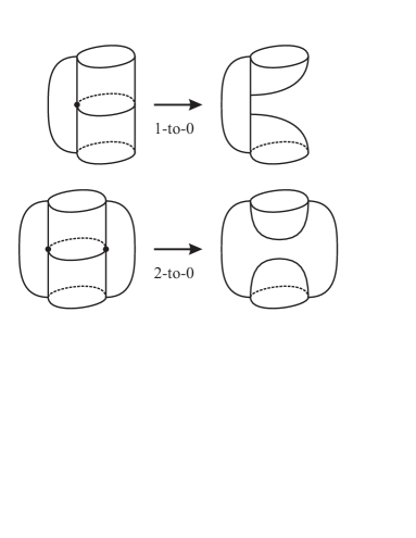
Figure 11: Moves on special spines turning them into simple ones.

can be applied is not a minimal spine of a prime $3$-manifold of positive complexity.

The proof of this result is given by Fig. 11 itself, because the moves described in it preserve the property that a polyhedron be a spine of a manifold, they lead to simple polyhedra, and they reduce the number of vertices.

According to Theorem 4.2(2) and Proposition 4.3, given $n\geq 1$, to produce the list of closed irreducible $3$-manifolds of complexity $n$, one can proceed according to the following (partly simultaneous) steps:

• Recursively construct the list of all orientable special spines with $n$ vertices of closed manifolds (or, dually, the list of all triangulations with $n$ tetrahedra of closed orientable manifolds);

• During the construction, check whether the configurations of Fig. 11 appear in incompletely constructed spines and, if so, discard automatically all their possible completions;

• Once a reduced list of spines has been obtained, eliminate duplications of manifolds by repeated applications of the $2$-to-$3$ move and its inverse, and show that the final list contains distinct manifolds using some invariants (such as homology or the Turaev-Viro invariants [56]).

This strategy has been carried out by Matveev for $n\leq 8$, by Martelli and the author for $n=9$ (using a substantial refinement [36] of Proposition 4.3, based on a certain theory of bricks), and then independently by Martelli and Matveev (see [35] and the references quoted there) for larger values of $n$. We also mention that Matveev and Tarkaev [40] have written a software, based on special spines and on the idea of applying moves to simplify them, that allows to recognize any given closed manifold in a very efficient way; the web site [40] also includes very helpful electronic lists of manifolds. In addition, non-orientable versions of the census have been obtained by Amendola and Martelli [3, 4] (using results of Martelli and the author [37] on non-orientable bricks) and by Burton [9, 10].

Closed hyperbolic manifolds

Matveev showed with a (complicated) theoretical argument that no closed manifold of complexity smaller than $9$ can be hyperbolic. The following was proved in [36]:

Theorem 4.4.

There are precisely $4$ closed orientable hyperbolic $3$-manifolds of complexity $9$, and they coincide with those of smallest known volume.

The $4$ manifolds referred to in the previous statement include the Weeks manifold, now known to be the minimum-volume closed orientable hyperbolic one, thanks to a result of Milley [41] based on his joint work with Gabai and Meyerhoff on Mom’s [23]. Martelli [35] found $25$ hyperbolic manifolds in complexity $10$, and Martelli and Matveev found (the same!) few more in higher complexity.

To conclude we mention that two completely alternative approaches to closed hyperbolic manifolds exist but will not be reviewed here. On one hand one can obtain a wealth of them doing Dehn filling on cusped manifolds (see Theorem 2.3), which SnapPea [61] allows to do very efficiently. On the other hand one can try to construct a hyperbolic structure on a given closed manifold, starting from a triangulation and using a method suggested by Casson [12] (see also Manning [34]).

5 Geodesic boundary and graphs

As many of the ideas in the realm of hyperbolic geometry, those underlying the algorithmic hyperbolization of manifolds with boundary are again due to Thurston [54], who first constructed such a structure on the complement of a graph in the $3$-sphere. As in the case of cusped manifolds, where one starts from some hyperbolic tetrahedra and imposes matching and completeness of the structure induced on the manifold obtained by gluing them, one starts from certain parameterized building blocks and tries to solve a system of equations. To describe the building blocks we will need a model of hyperbolic space not employed so far, namely the projective model, obtained by projecting radially (whence the name) the hyperboloid ${\mathcal{H}}^{n}_{+}$ to the unit disc $B^{n}_{\mathbb{P}}$ of the hyperplane at height $x_{0}=1$ in Minkowski space ${\mathbb{R}}^{1,n}$. The main advantage of this model is that hyperbolic straight lines appear as Euclidean straight segments in it (but the angles are not the Euclidean ones, as it happens instead in the disc and half-space models).

We define a hyperideal hyperbolic polyhedron as a polyhedron $P$ in the space ${\mathbb{R}}^{n}$ containing $B^{n}_{\mathbb{P}}$ so that:

• $P$ has some hyperideal vertices, lying outside the closure of $B^{n}_{\mathbb{P}}$, and possibly some ideal ones, lying on the boundary of $B^{n}_{\mathbb{P}}$;

• $P$ has some genuine edges, meeting the interior of $B^{n}_{\mathbb{P}}$, and possibly some ideal edges, tangent at one point to the boundary of $B^{n}_{\mathbb{P}}$;

• The ends of each ideal edge are hyperideal (i.e., not ideal) vertices of $P$.

To such a $P$ we will always associate the corresponding truncated hyperideal hyperbolic polyhedron $\widehat{P}$, to define which we introduce for each hyperideal vertex $v$ of $P$:

• The $(n-1)$-sphere $\gamma_{v}\subset\partial B^{n}_{\mathbb{P}}$ of the tangency points to $\partial B^{n}_{\mathbb{P}}$ of lines emanating from $v$;

• The hyperplane $\alpha_{v}$ in $\{1\}\times{\mathbb{R}}^{n}\subset{\mathbb{R}}^{1,n}$ containing $\gamma_{v}$;

• The closed half-space $Q_{v}$ in $\{1\}\times{\mathbb{R}}^{n}$ bounded by $\alpha_{v}$ and not containing $v$.

Then we define the truncation $\widehat{P}$ of $P$ as the intersection of $P$ with the $Q_{v}$’s as $v$ varies among the hyperideal vertices of $P$. See Fig. 12 for $2$-dimensional examples of $P$ and $\widehat{P}$.

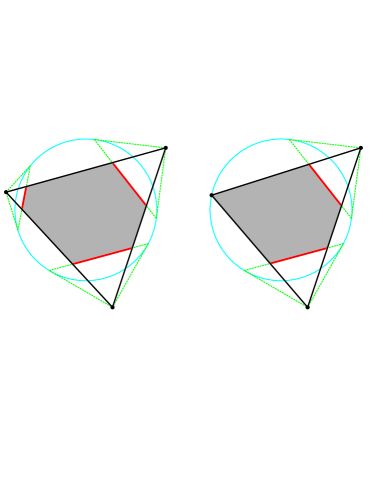
Figure 12: A genuine hyperideal triangle and its truncation; a hyperideal triangle with an ideal vertex and its truncation; a hyperideal triangle with an ideal edge and its truncation.

Note that one can naturally define for a truncated hyperideal hyperbolic polyhedron the truncation faces as those lying on the $\alpha_{v}$’s, and the lateral faces, coming from the original ones. The following fact is easy to show:

Lemma 5.1.

The truncation faces and the lateral faces of a truncated hyperideal hyperbolic polyhedron lie at right angles to each other.

This implies that the hexagon in Fig. 12-left is right-angled (even if one would not be able to tell from the picture), and that the two pentagons in Fig. 12-center and -right are right-angled at the non-ideal vertices.

Turning to dimension $3$, the next result follows from the previous one and will be needed below:

Lemma 5.2.

If $v$ is the ideal point at which an ideal edge of a truncated hyperideal hyperbolic polyhedron $\widehat{P}$ meets $\partial B^{3}_{\mathbb{P}}$, then the intersection of $\widehat{P}$ with a sufficiently small horosphere centered at $v$ is a Euclidean rectangle.

Moduli and hyperbolicity equations

Let us from now on restrict our discussion to dimension $3$. Given a compact manifold $M$ with boundary, or more generally a pair $(M,{\mathcal{A}})$ where ${\mathcal{A}}\subset\partial M$ is a family of closed annuli, one tries to construct on $M$ a hyperbolic structure such that the non-toric components of $\partial M\setminus{\mathcal{A}}$ are totally geodesic (so the components of ${\mathcal{A}}$ give annular cusps, whereas the tori give toric cusps). The way to do this algorithmically is again to start from an ideal triangulation ${\mathcal{T}}$, encode by certain modules the structures of truncated hyperideal hyperbolic tetrahedra one can put on the tetrahedra of ${\mathcal{T}}$, and try to solve certain equations on the modules that translate the fact that the structures of the tetrahedra match to give a global complete hyperbolic structure on $M$ of the appropriate type. As for modules, the following was shown in [22] (see also [21]):

Proposition 5.3.

The space of modules for a hyperideal hyperbolic tetrahedron is given by the $6$ dihedral angles, that vary freely subject to the following restrictions:

• The sum of the angles at a hyperideal vertex is less than $\pi$;

• The sum of the angles at an ideal vertex is equal to $\pi$;

• The angle at an ideal edge is $0$.

Since this will be needed soon, we also mention that, given a choice of modules for a hyperideal hyperbolic tetrahedron $\Delta$, the lengths of all the lateral and truncation edges of the corresponding truncated $\widehat{\Delta}$ are computed by explicit formulae to be found in [21]. Note that an ideal edge always has length $0$, and an edge with one or both ideal ends has length $+\infty$.

Turning to the global matching of the structures on the individual tetrahedra of a triangulation, we begin from the case of a pair $(M,{\mathcal{A}})$ with ${\mathcal{A}}=\emptyset$, where one starts from an ideal triangulation ${\mathcal{T}}$ of a compact $M$ in the usual sense. (The case ${\mathcal{A}}\neq\emptyset$ requires important variations discussed below.) In this case the matching equations express the fact that the lengths of all the truncation and lateral edges should be matched by the gluings of ${\mathcal{T}}$. But, as a matter of fact, since a right-angled hyperbolic hexagon with finite vertices is determined by the lengths of three pairwise non-consecutive edges, the requirement that all lengths should be matched is typically redundant.

As just described, the matching equations for hyperideal tetrahedra are quite different than those for ideal tetrahedra. In particular, we stress that the formulae to compute the lengths of the edges involve trigonometric and hyperbolic functions, so the equations are not algebraic ones. On the other hand the completeness equations are precisely the same: the modules give Euclidean structures up to similarity on the triangles of which each boundary torus is constituted, and completeness translates into the fact that each such torus should be Euclidean, and in turn into explicit equations in the modules along the lines of Proposition 3.4.

Annular cusps

For a pair $(M,{\mathcal{A}})$ with ${\mathcal{A}}\subset\partial M$ a family of closed annuli, the approach to hyperbolization using triangulations requires an important variation. To understand it, suppose that $(M,{\mathcal{A}})$ has a decomposition ${\mathcal{T}}$ into truncated hyperideal hyperbolic tetrahedra. Then an annular cusp $A\in{\mathcal{A}}$ corresponds to an ideal edge of ${\mathcal{T}}$. More precisely, one obtains the compact pair $(M,{\mathcal{A}})$ by first taking the compact manifold obtained by gluing the truncated versions of the tetrahedra in ${\mathcal{T}}$, and then digging open cylindrical tunnels along the edges of ${\mathcal{T}}$. This means that ${\mathcal{T}}$ itself is not an ideal triangulation of $M$. On the contrary, the following holds:

Proposition 5.4.

The ideal triangulations required to hyperbolize a pair $(M,{\mathcal{A}})$ are those of the form $({\mathcal{T}},a)$, where:

• ${\mathcal{T}}$ is an ideal triangulation of the manifold $N$ described next, and $a$ is a family of edges of ${\mathcal{T}}$;

• $N$ is the manifold obtained from $M$ by gluing a solid cylinder (a $2$-handle) to each annulus in ${\mathcal{A}}$;

• The family of edges $a$, viewed in $N$, is precisely the family of cores of the solid cylinders glued to $M$ to get $N$;

• When choosing modules for the tetrahedra in ${\mathcal{T}}$, the ideal edges should be precisely those in $a$.

The case with annular cusps requires the initial subtlety just described, and one more. The point is that there is one very special case where two “hexagons” with the same ordered lengths of the edges need not be isometric, so the matching of lengths of the edges is not sufficient to ensure consistency of the hyperbolic structure carried by a choice of modules for the tetrahedra in a triangulation, and an additional equation must be added. This occurs when a hexagon has one ideal edge and an opposite ideal vertex, so it reduces to a quadrilateral with two ideal and two finite vertices. The extra parameter describing the shape of such an object is described in [21] together with the method to compute it starting from the modules.

Fortunately enough, after these two complications, we can show that in dealing with annular cusps no completeness issues arise:

Proposition 5.5.

Consider a (possibly incomplete) hyperbolic structure on $(M,{\mathcal{A}})$ given by a solution of the matching equations for a triangulation $({\mathcal{T}},a)$ as in the previous result. Then the structure is automatically complete at the annular cusps ${\mathcal{A}}$.

Proof.

By Lemma 5.2 a horospherical cross-section at some $A\in{\mathcal{A}}$ is obtained by gluing some rectangles, so it is a Euclidean annulus with boundary components of equal length. The double of such an annulus is a Euclidean torus (and not merely a similarity one), and the conclusion easily follows from Proposition 3.3. ∎

Canonical decomposition

The recognition of hyperbolic $3$-manifolds with geodesic boundary is based on an analogue for this type of manifolds of the Epstein-Penner canonical decomposition, due to Kojima [31, 32]. For a pair $(M,{\mathcal{A}})$ without toric cusps (but ${\mathcal{A}}$ can be non-empty, so annular cusps are allowed) the Kojima decomposition is a subdivision of $M$ into truncated hyperideal hyperbolic polyhedra, possibly with ideal edges but without ideal vertices, and it is simply dual to the cut-locus of the boundary, as illustrated in Fig. 10. This definition is of course of impractical use, but Kojima proved an analogue of Proposition 3.9 that allows the actual computation of the canonical decomposition. To state this result we need to recall more of the geometry of the hyperboloid model ${\mathcal{H}}^{n}_{+}$ of hyperbolic space. We define the $1$-sheeted hyperboloid

$${\mathcal{S}}^{n}=\{y\in{\mathbb{R}}^{1,n}:\ \left\langle x|x\right\rangle_{(1,n)}=+1\}$$

and, for $y\in{\mathcal{S}}^{n}$,

$$Q_{y}=\{x\in{\mathcal{H}}^{n}_{+}:\ \left\langle x|y\right\rangle_{(1,n)}\leq 0\},$$

noting that $Q_{y}$ is a geodesic half-space in ${\mathcal{H}}^{n}_{+}$, and that each such half-space has the form $Q_{y}$ for a unique $y\in{\mathcal{S}}^{n}$.

Let us now consider a hyperbolic $(M,{\mathcal{A}})$ without toric cusps and recall that the hyperbolic structure induces an identification between its universal cover and an intersection of closed geodesic half-spaces in ${\mathbb{H}}^{3}$. Using the hyperboloid model ${\mathcal{H}}^{3}_{+}$ we then have $\widetilde{M}=\bigcap\{Q_{y}:\ y\in{\mathcal{P}}\}$ for some family of points ${\mathcal{P}}\subset{\mathcal{S}}^{3}$. As in the cusped case we now define $C$ as the convex hull of ${\mathcal{P}}$ in ${\mathbb{R}}^{1,3}$. Kojima proved the following result, stated in a rather informal way here (but carefully stated and proved in [21]):

Proposition 5.6.

If $(M,{\mathcal{A}})$ is hyperbolic without toric cusps then the canonical decomposition of $(M,{\mathcal{A}})$ dual to the cut-locus of the boundary is obtained by projecting radially to ${\mathcal{H}}^{3}_{+}$ the faces of $\partial C$ that meet the positive time-like half-lines.

Turning to the case of a hyperbolic manifold with geodesic boundary $(M,{\mathcal{A}})$ also having toric cusps, we briefly mention that a canonical decomposition has been constructed by Kojima also in this case. The argument is somewhat more complicated, the main steps being as follows:

• Let ${\mathcal{P}}_{\mathcal{S}}\subset{\mathcal{S}}^{3}$ be the family of points such that the universal cover of $(M,{\mathcal{A}})$ is $\bigcap\{Q_{y}:\ y\in{\mathcal{P}}_{\mathcal{S}}\}$;

• Let ${\mathcal{P}}_{\mathcal{L}}\subset{\mathcal{L}}^{3}_{+}$ be the family of points such that the family of horoballs $\{B_{y}:\ y\in{\mathcal{P}}_{\mathcal{L}}\}$ projects in $(M,{\mathcal{A}})$ to a family of equal-volume “sufficiently small” disjoint toric cusps;

• Let ${\mathcal{P}}={\mathcal{P}}_{\mathcal{S}}\cup{\mathcal{P}}_{\mathcal{L}}$ and define $C$ as the convex hull in ${\mathbb{R}}^{1,3}$ of ${\mathcal{P}}$;

• Then the canonical decomposition of $(M,{\mathcal{A}})$ is obtained by projecting radially to ${\mathcal{H}}^{3}_{+}$ the faces of $\partial C$ that meet the positive time-like half-lines, and then suitably subdividing those arising from vertices in ${\mathcal{P}}_{\mathcal{L}}$.

We only mention that how small the toric cusps should be in order for this construction to work was left implicitly determined by Kojima, and was later spelled out in a quantitative fashion in [21].

Algorithmic recognition

While enumerating some class of hyperbolic manifolds with geodesic boundary, for each manifold one constructs the structure using a triangulation (which, in practice, always works for minimal triangulations if there are no topological obstructions to hyperbolicity), and then one is faced with the issue of algorithmically finding the Kojima canonical decomposition. The strategy to do so is the same as in the cusped context: starting from the given triangulation one tries to decide whether its tetrahedra represent the projections of the faces of $\partial C$, which amounts to checking whether the angles between suitable liftings of the tetrahedra, determined by the global geometry, are convex if viewed from the origin. And this can be carried out using an extension of the Sakuma-Weeks tilt formula, due to Usijima [57] and carefully described in [21]. If some concave angle is found the combinatorics of the triangulation is changed by performing the $2$-to-$3$ move along the offending face, until the process gets stuck (which never happens in practice) or the Kojima decomposition is reached.

Experimental results

The framework described above was successfully used by Frigerio, Martelli and the author [19] to list all manifolds with non-empty geodesic boundary and (possibly) toric cusps, but no annular cusp, that can be triangulated with up to $4$ tetrahedra. The data are available online [20] and include the computation of the volume, based on results of Ushijima [58].

One of the most striking findings of [19] is that there are $56$ manifolds whose canonical Kojima decomposition consists of a single hyperideal regular octahedron (with different combinatorics of the gluings). The corresponding $56$ manifolds share the same volume and would be extremely difficult to distinguish from each other using different techniques (such as the invariants of algebraic topology or those of Turaev and Viro): it is only using hyperbolic geometry in its full power that one can tell that they are actually distinct. We also mention that this result naturally prompted the problem of enumerating all the different manifolds that can be obtained gluing the faces of the octahedron, solved by Heard, Pervova and the author in [27].

Turning to graphs, the trivalent hyperbolic ones in the most general sense (with parabolic meridians) were investigated by Heard, Hodgson, Martelli and the author in [26], where (with the restriction that each graph should have at least one trivalent vertex) all those that can be triangulated by $5$ or less tetrahedra were enumerated and carefully analized. The enumeration and analysis have exploited Heard’s excellent software [25], which allows to hyperbolize and study manifolds with boundary and orbifolds in an extremely effective fashion.

No systematic enumeration of hyperbolic orbifolds has been carried out so far, but the theoretical and computer methods are all in place, as described above, and the author is hoping to contribute to the topic in the future.

Dipartimento di Matematica Applicata
Via Filippo Buonarroti, 1C
56127 PISA – Italy
petronio@dm.unipi.it

References

- [1] C. C. Adams, Thrice-punctured spheres in hyperbolic -manifolds, Trans. Amer. Math. Soc. 287 (1985), 645-656.
- [2] G. Amendola, A calculus for ideal triangulations of three-manifolds with embedded arcs, Math. Nachr. (9) 278 (2005), 975-994.
- [3] G. Amendola – B. Martelli, Non-orientable -manifolds of small complexity, Topology Appl. 133 (2003), 157-178.
- [4] G. Amendola – B. Martelli, Non-orientable -manifolds of complexity up to , Topology Appl. 150 (2005), 179-195 .
- [5] R. Benedetti – C. Petronio, “Lectures on Hyperbolic Geometry,” Springer-Verlag, Berlin-Heidelberg-New York, 1992.
- [6] R. Benedetti – C. Petronio, A finite graphic calculus for -manifolds, Manuscripta Math. 88 (1995), 291-310.
- [7] L. Bessières – G. Besson – M. Boileau – S. Maillot – J. Porti, Weak collapsing and geometrisation of aspherical -manifolds, arXiv:0706.2065v2 [math.GT] 28 Jan 2008.
- [8] M. Boileau – B. Leeb – J. Porti, Geometrization of -dimensional orbifolds, Ann. of Math. (2) 162 (2005), 195-290.
- [9] B. A. Burton, Enumeration of non-orientable -manifolds using face-pairing graphs and union-find, Discrete Comput. Geom. 38 (2007), 527-571 .
- [10] B. A. Burton, Observations from the -tetrahedron nonorientable census, Experiment. Math. 16 (2007), 129-144.
- [11] P. J. Callahan – M. V. Hildebrandt – J. R. Weeks, A census of cusped hyperbolic -manifolds, with microfiche supplement, Math. Comp. 68 (1999), 321-332.
- [12] A. J. Casson, unpublished.
- [13] A. J. Casson – D. S. Jungreis, Convergence groups and Seifert fibered -manifolds, Invent. Math. 118 (1994), 441-456.
- [14] D. Cooper – C. D. Hodgson – S. P. Kerckhoff, “Three-dimensional orbifolds and cone-manifolds”, MSJ Memoirs, Vol. 5, Mathematical Society of Japan, Tokyo, 2000.
- [15] M. P. do Carmo “Riemannian Geometry,” Mathematics: Theory & Applications, Birkhäuser Boston, Inc., Boston, MA, 1992.
- [16] D. B. A. Epstein – R. C. Penner, Euclidean decomposition of non-compact hyperbolic manifolds, J. Differential Geom. (1) 27 (1988), 67-80.
- [17] A. T. Fomenko – S. V. Matveev, “Algorithmic and Computer Methods for Three-Manifolds,” Mathematics and its Applications, Vol. 425, Kluwer Academic Publishers, Dordrecht, 1997.
- [18] R. Frigerio, Hyperbolic manifolds with geodesic boundary which are determined by their fundamental group, Topology Appl. 145 (2004), 69-81.
- [19] R. Frigerio – B. Martelli – C. Petronio, Small hyperbolic -manifolds with geodesic boundary, Experiment. Math. 13 (2004), 171-184.
- [20] R. Frigerio – B. Martelli – C. Petronio, “Hyperbolic -manifolds with non-empty geodesic boundary,” Tables available from www.dm.unipi.it/pages/petronio/public-html.
- [21] R. Frigerio – C. Petronio, Construction and recognition of hyperbolic -manifolds with geodesic boundary, Trans. Amer. Math. Soc. 356 (2004), 3243-3282.
- [22] M. Fujii, Hyperbolic -manifolds with totally geodesic boundary which are decomposed into hyperbolic truncated tetrahedra, Tokyo J. Math. 13 (1990), 353-373.
- [23] D. Gabai – R. G. Meyerhoff – P. Milley, Mom technology and hyperbolic -manifolds, to appear in the Proceedings of the 2008 Ahlfors-Bers Colloquium (AMS Contemporary Mathematics series).
- [24] O. Goodman, “Snap,” The computer program for studying arithmetic invariants of hyperbolic 3-manifolds, available from http://www.ms.unimelb.edu.au/snap/ and from http://sourceforge.net/projects/snap-pari.
- [25] D. Heard, “Orb,” The computer program for finding hyperbolic structures on hyperbolic 3-orbifolds and 3-manifolds, available from http://www.ms.unimelb.edu.au/snap/orb.html.
- [26] D. Heard – C. Hodgson – B. Martelli – C. Petronio, Hyperbolic graphs of small complexity, arXiv:0804.4790v1 [math.GT], 35 pages, to appear in Experiment. Math.
- [27] D. Heard – E. Pervova – C. Petronio, The orientable octahedral manifolds, Experiment. Math. 17 (2008), 473-486.
- [28] J. Hempel, “3-Manifolds,” Ann. of Math. Studies, Vol. 86, Princeton, 1976.
- [29] W. Jaco, “Lectures on Three-Manifold Topology,” CBMS Regional Conference Series in Mathematics, Vol. 4, American Mathematical Society, Providence, R.I., 1980.
- [30] R. C. Kirby – L. C. Siebenmann, “Foundational Essays on Topological Manifolds, Smoothings, and Triangulations,” Princeton University Press, Princeton, NJ, 1977.
- [31] S. Kojima, Polyhedral decomposition of hyperbolic manifolds with boundary, Proc. Work. Pure Math. 10 (1990), 37-57.
- [32] S. Kojima, Polyhedral decomposition of hyperbolic -manifolds with totally geodesic boundary, In: “Aspects of Low-Dimensional Manifolds,” Adv. Stud. Pure Math. Vol. 20, Kinokuniya, Tokyo, 1992, 93-112.
- [33] F. Luo – S. Schleimer – S. Tillmann, Geodesic ideal triangulations exist virtually, Proc. Amer. Math. Soc. 136 (2008), 2625-2630.
- [34] J. Manning, Algorithmic detection and description of hyperbolic structures on closed -manifolds with solvable word problem, Geom. Topol. 6 (2002), 1-25.
- [35] B. Martelli, Complexity of -manifolds, In: “Spaces of Kleinian Groups”, London Math. Soc. Lecture Note Ser., Vol. 329, Cambridge Univ. Press, Cambridge, 2006, 91-120.
- [36] B. Martelli – C. Petronio, -manifolds having complexity at most , Experiment. Math. 10 (2001), 207-237.
- [37] B. Martelli – C. Petronio, A new decomposition theorem for -manifolds, Illinois J. Math. 46 (2002), 755-780.
- [38] S. V. Matveev, Complexity theory of three-dimensional manifolds, Acta Appl. Math. 19 (1990), 101-130.
- [39] S. V. Matveev, “Algorithmic Topology and Classification of -Manifolds,” ACM-monographs Vol. 9, Springer-Verlag, Berlin-Heidelberg-New York, 2003.
- [40] S. V. Matveev – V. V. Tarkaev, “Three-manifold Recognizer”, A computer program for recognition of 3-manifolds, available from http://www.matlas.math.csu.ru with electronic tables of -manifolds.
- [41] P. Milley, Minimum volume hyperbolic -manifolds, J. Topol. 2 (2009), 181-192.
- [42] J. Milnor, Hyperbolic geometry: the first 150 years, Bull. Amer. Math. Soc. (N.S.) 6 (1982), 9-24
- [43] W. D. Neumann – D. Zagier, Volumes of hyperbolic three-manifolds, Topology 24 (1985), 307-332.
- [44] G. Perelman, The entropy formula for the Ricci flow and its geometric applications, preprint math.DG/0211159.
- [45] G. Perelman, Ricci flow with surgery on three-manifolds, preprint math.DG/0303109.
- [46] G. Perelman, Finite extinction time for the solutions to the Ricci flow on certain three-manifolds, preprint math.DG/0307245.
- [47] E. Pervova – C. Petronio, Complexity of links in -manifolds, J. Knot Theory Ramifications 18 (2009), 1439-1458.
- [48] C. Petronio – J. Porti, Negatively oriented ideal triangulations and a proof of Thurston’s hyperbolic Dehn filling theorem, Exposition. Math. 18 (2000), 1-35.
- [49] C. Petronio – J. R. Weeks, Partially flat ideal triangulations of cusped hyperbolic -manifolds, Osaka J. Math. 37 (2000), 453-466.
- [50] R. Piergallini, Standard moves for standard polyhedra and spines, Rend. Circ. Mat. Palermo (II) 18 Suppl. (1988), 391-414
- [51] J. G. Ratcliffe, “Foundations of Hyperbolic Manifolds,” Second Edition, Graduate Texts in Math. Vol. 149, Springer-Verlag, New York, 2006.
- [52] C. P. Rourke – B. J. Sanderson, “Introduction to Piecewise-Linear Topology,” Ergebn. der Math. Vol. 69, Springer-Verlag, New York-Heidelberg, 1972.
- [53] M. Sakuma – J. R. Weeks, The generalized tilt formula, Geom. Dedicata 50 (1995), 1-9.
- [54] W. P. Thurston, “The Geometry and Topology of -manifolds,” mimeographed notes, Princeton, 1979; see also “Three-Dimensional Geometry and Topology. Vol. 1,” Edited by Silvio Levy, Princeton Mathematical Series, Vol. 35, Princeton University Press, Princeton, NJ, 1997.
- [55] W. P. Thurston, Hyperbolic structures on -manifolds. I. Deformation of acylindrical manifolds, Ann. of Math. (2) 124 (1986), 203-246.
- [56] V. G. Turaev – O. Ya. Viro, State sum invariants of -manifolds and quantum -symbols, Topology (4) 31 (1992), 865-902.
- [57] A. Ushijima, The tilt formula for generalized simplices in hyperbolic space, Discrete Comput. Geom. 28 (2002), 19-27.
- [58] A. Ushijima, A volume formula for generalised hyperbolic tetrahedra, In: “Non-Euclidean Geometries”, Mathematics and Its Applications, Vol. 581, Springer, NY, 2006, 249-265.
- [59] M. Wada – Y. Yamashita – H. Yoshida, An inequality for polyhedra and ideal triangulations of cusped hyperbolic -manifolds, Proc. Amer. Math. Soc. 124 (1996), 3905–3911.
- [60] J. R. Weeks, Convex hulls and isometries of cusped hyperbolic -manifolds, Topology Appl. 52 (1993), 127-149.
- [61] J. R. Weeks, “SnapPea”, The hyperbolic structures computer program, available from www.geometrygames.org.