New Completeness Methods for Estimating Exoplanet Discoveries by Direct Detection

Abstract

We report new methods for evaluating realistic observing programs that search stars for planets by direct imaging, where observations are selected from an optimized star list, and where stars can be observed multiple times. We show how these methods bring critical insight into the design of the mission and its instruments. These methods provide an estimate of the outcome of the observing program: the probability distribution of discoveries (detection and/or characterization), and an estimate of the occurrence rate of planets ($\eta$). We show that these parameters can be accurately estimated from a single mission simulation, without the need for a complete Monte Carlo mission simulation, and we prove the accuracy of this new approach. Our methods provide the tools to define a mission for a particular science goal, for example defined by the expected number of discoveries and its confidence level. We detail how an optimized star list can be built and how successive observations can be selected. Our approach also provides other critical mission attributes, such as the number of stars expected to be searched, and the probability of zero discoveries. Because these attributes depend strongly on the mission scale (telescope diameter, observing capabilities and constraints, mission lifetime, etc.), our methods are directly applicable to the design of such future missions and provide guidance to the mission and instrument design based on scientific performance. We illustrate our new methods with practical calculations and exploratory design reference missions (DRMs) for the James Webb Space Telescope (JWST) operating with a distant starshade to reduce scattered and diffracted starlight on the focal plane. We estimate that 5 habitable Earth-mass planets would be discovered and characterized with spectroscopy, with a probability of zero discoveries of 0.004, assuming a small fraction of JWST observing time (7%), $\eta=0.3$, and 70 observing visits, limited by starshade fuel.

1 Introduction

Various proposals for direct-imaging searches for Earth-like planets are now on the table (Guyon et al., 2008; Cash et al., 2008; Spergel et al., 2009; Soummer et al., 2009b). This paper presents methods to guide the development of the new instrumentation that such searches will require. They can also help optimize observing programs by scheduling observations to maximize their impact. Using these new methods, we can predict the outcome of a single observation or an entire observing program, and interpret the observational results. These tools should be widely useful for studying, comparing, and optimizing alternative direct-search concepts.

The completeness of a direct limiting search observation (LSO) is the fraction of all possible planets of interest (POIs) that satisfy the detection criteria. By definition, an LSO has sufficient exposure time, $t_{\mathrm{exp},j}$ on the $j^{\mathrm{th}}$ star, to reach the systematic limit of the instrument. For optical missions, an LSO is assumed to achieve the desired photometric signal-to-noise ratio on the limiting source, which has magnitude mag${}_{j}+\Delta\textit{mag}_{0}$, where mag_j is the stellar magnitude, and $\Delta\textit{mag}_{0}$ is the limiting magnitude difference with the star (flux contrast), expected to be determined by speckle instability (Brown, 2005).

In the simplest picture, an LSO discovers any and all POIs that satisfy two criteria at the time of the observation:

$$\Delta\textit{mag}<\Delta\textit{mag}_{0}~{},$$ (1)

and

$$s>\textit{IWA}~{},$$ (2)

where $s$ is the angular separation between planet and star, and IWA is the inner working angle (angular radius of the real or effective central field obscuration). This simplified picture of a sharp dividing line between detectable and undetectable planets has proven useful for measuring search power to first order. Fidelity could be improved, if necessary, by adding more complex detection criteria, such as a detection probability that varies in a more complicated and realistic way over the field of view.

In a common treatment, which we follow here, the POIs are body-twins of Earth with orbits in the habitable zone.

Let a fraction $\eta$ of all stars in the universe have a POI. The list of candidate stars for the observing program is a subset of all stars, and within this subset, the expected fraction is $\eta$, but the actual fraction will vary. Also, we have limited knowledge of $\eta$, a number that is both interesting scientifically and useful operationally to schedule observations to maximize discoveries. Therefore, we will draw distinctions when necessary between the true value ($\eta_{\mathrm{true}}$), which is unknown, the assumed value for science operations ($\eta_{\mathrm{ops}}$), which is used to estimate discovery probabilities, and the value estimated from the results of a search program [$E(\eta)$].

Our new methods extend the original concept of direct-search completeness for exoplanets (Brown, 2004, 2005) for purposes of optimizing the timing of revisits to previously searched stars, increasing the realism of instrument comparisons, and providing an estimate of $\eta$ from the results of observing programs. Meanwhile, Brown (2009a, b) has extended completeness studies to indirect detection by reflex astrometry, photometric detection in the case of no occultations, and the estimation of orbital parameters from Keplerian data sets.

2 Evolution and Estimation of Completeness

2.1 Four Types of Completeness

Four types of completeness pertain to a program of LSOs: virgin, dynamic, accumulated, and ultimate.

Until now, the scheduling of LSOs in mission studies of direct-search power has been based on “virgin,” time-independent, first-visit completeness $c_{1,j}$, which is the completeness of the first LSO of star $j$ (Brown, 2004; Agol, 2007; Savransky, Kasdin, & Cady, 2010). In this study, we include the possibility of multiple LSOs of any target star.

A non-detection by an LSO rules out some fraction of possible planets: those with sufficient angular separation and brightness at the time $t$ of the LSO to be detectable—if they existed. After the LSO, a pool of possible planets may remain, comprising planets that had not been ruled out by previous LSOs and also were not detectable by the most recent LSO. As time goes on, each planet in this pool moves along its unique orbit and may become detectable at some future time. In this way, the fraction of all possible planets that is detectable on the $i^{\mathrm{th}}$ visit to the $j^{\mathrm{th}}$ star at time $t$—which is the dynamic completeness, $c_{i,j}(t)$—depends on the elapsed time since each of the $i-1$ preceding LSOs.

Accumulated completeness ($C_{i,j}$) is the sum-total completeness of $i$ LSOs of star $j$:

$$C_{i,j}\equiv\sum\limits_{l=1}^{i}{c_{l,j}(t_{l})}~{}.$$ (3)

$C_{i,j}$ increases monotonically with $i$.

Ultimate completeness ($C_{\infty,j})$ is the maximum value of $C_{i,j}$. It is the value of completeness that would be accumulated from an arbitrarily high number of LSOs spread arbitrarily over time:

$$C_{\infty,j}=\sum\limits_{l=1}^{\infty}{c_{l,j}(t_{l})}~{}.$$ (4)

$C_{\infty,j}<1$ whenever some POI orbits are permanently fainter than $\Delta\textit{mag}_{0}$ or permanently obscured inside IWA—or never brighter than $\Delta\textit{mag}_{0}$ and located outside IWA at the same time.

2.2 Estimating Dynamic Completeness $c_{i,j}$

All types of completeness are derived from $c_{i,j}$, and all results (probability of discovery and mission outcomes) are ultimately based on this quantity.

Because the planetary position is determined by a transcendental equation (Kepler’s Equation), $c_{i,j}$ must be estimated by Monte Carlo trials. In these trials, we represent the universe of POIs by a large random sample of $N_{0}$ particular POIs, each of which is defined by randomly chosen values for ten parameters: $\{a$, $e$, $M_{0}$, $i$, $\omega_{\mathrm{p}}$, $\Omega$, ${\cal T}$, $R_{\mathrm{p}}$, $q$, $\Phi\}$, where $a$ is the semimajor axis, $e$ is the orbital eccentricity, $M_{0}$ is the mean anomaly at some definite time, $i$ is the inclination angle, $\omega_{\mathrm{p}}$ is the argument of periastron, $\Omega$ is the position angle of the ascending node, ${\cal T}$ is the orbital period, $R_{\mathrm{p}}$ is the planetary radius, $q$ is the geometric albedo, and $\Phi$ comprises the necessary sub-parameters for defining the phase function.

In this paper, the POIs are Earth-twins on habitable-zone orbits. The particular values of six parameters are drawn from random deviates: $0.7\sqrt{L}\leq a\leq 1.5\sqrt{L}$, $0\leq e\leq 0.35$, and $0\leq M_{0}\leq 2\pi$ (uniformly distributed; $L$ is the stellar luminosity); $i$, $\omega_{\mathrm{p}}$, and $\Omega$ uniformly distributed on the sphere. Three parameters are delta functions: $R_{\mathrm{p}}=R_{\oplus}$, $q$ depends on the filter passband, and $\Phi$ is the Lambertian phase function. ${\cal T}$ is given by $a$ and the stellar mass via Kepler’s Third Law.

When estimating $c_{1,j}$, for the first LSO, $\Delta$mag and $s$ are computed for all $N_{0}$ POIs at, say, $t=0$, when the orbital phases of all POIs in the sample are equal to $\{M_{0}\}$. Thereafter, record is kept of the epoch of each LSO, $t_{i>1}$, only for the POIs that have not yet been eliminated and are still in play.

For the $i^{\mathrm{th}}$ LSO, we identify and count the number of POIs that satisfy Eqs. (1–2), $N_{i,j}$, producing:

$$c_{i,j}=\frac{N_{i,j}}{N_{0}}~{}.$$ (5)

Based on Eq. (5), all types of completeness can be computed with any required precision by appropriately choosing the value of $N_{0}$.

2.3 Rebound of $c_{i,j}$

$c_{i+1,j}(t)$ rebounds following the $i^{\mathrm{th}}$ LSO. $c_{i+1,j}(t_{i}+\epsilon)=0$, where $\epsilon$ is a diminishingly small increment of time, and then it rebounds towards a constant, asymptotic value, $c_{i+1,j}(\infty)$, as the orbits of still-possible POIs lose orbital phase coherence.

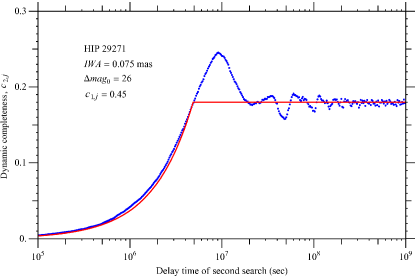
Figure 1: Typical rebound of dynamic completeness $c_{2,j}(t)$ following the first limiting search observation (LSO) at $t=0$. Blue: values calculated from Eq. 5 with $N_{0}=20,000$, for Earth-like, habitable-zone planets around HIP 29271, assuming IWA = 0.075 arcsec, $q=0.26$, and $\Delta\textit{mag}_{0}=26$. Red: the linear approximation. Here, $c_{2,j}(\infty)=0.18$ and breaktime $=5\times 10^{7}$ sec.

The blue points in Figure 1 show how $c_{2,j}$ rebounds after a first LSO at $t=0$ of HIP 29271 for IWA = 0.075 arcsec (THEIA; Savransky, Kasdin, & Cady, 2010) $q=0.26$, and $\Delta\textit{mag}_{0}=26$ (typical value; Brown, 2005). The rebound resembles the response of the output voltage for an underdamped, series, LRC circuit after a step change in the input voltage. After a linear rise (curved on a logarithmic plot), $c_{2,j}$ undergoes damped oscillations. The details—rise time, damping time, and asymptotic value $c_{2,j}(\infty)$—depend on the star’s particular mix of habitable-zone orbits resolved by IWA. For different stellar mass, luminosity, and distance, for other values of IWA and $\Delta\textit{mag}_{0}$, and for other definitions of POIs, the rebound of $c_{2,j}$ will be qualitatively similar to Figure 1, but with different details and numbers. For example, other factors being equal, a star at larger distance would have a longer rebound time, because the central field obscuration (IWA) would limit the observation to planets with wider separations, and therefore a longer time would be necessary to loose orbit coherence.

When the next observation is being planned, we need to know $c_{i,j}(t)$ for each star in play, and where $i-1$ observations of star $j$ have already been performed. When $i=1$, we would use tabulated values of time-independent virgin completeness, and no real-time computation would be required. When $i>1$, however, we may need an efficient function or procedure for computing the values of $c_{i,j}(t)$.

The most accurate, brute-force method would perform a blue-point-type calculation (see Figure 1) for every star in play every time a new observation is planned. The number of times would be of order the number of stars times the number of observations. For example, the number of blue-point-type calculations would exceed $10^{5}$ for a program of 100 stars and 1,000 LSOs, typical for a 4-m class instrument with IWA $=0.075$ arcsec. Monte Carlo full-mission studies would be impractical, as each of the 400 blue points in Figure 1 took $\sim$5 sec to compute on a 3 GHz Intel Xenon processor running Mathematica 6. Therefore, we must look at two approximate functions for $c_{i,j}(t)$, one of which may be perfectly adequate for first-order scheduling studies. They demand only one or four blue-point-type calculations performed a number of times that is of order the number of observations.

The first alternative approximation is a linear function, $c_{i,j}(t)=\textit{slope}\times t$ for $t<\textit{breaktime}$, and $c_{i,j}(t)=c_{i,j}(\infty)$ for $t>\textit{breaktime}$. This is illustrated by the red curve in Figure 1.

We used the following algorithm to find the parameters slope and $\textit{breaktime}\equiv c_{i,j}(\infty)/$slope. The algorithm comprises four blue-point-type computations of $c_{i,j}(t)$. First, we estimate $c_{i,j}(\infty)$ by computing $c_{i,j}(10^{10}$ sec). Second, we compute $c_{i,j}(10^{5.5}$ sec), and use it to make a first estimate of the slope, $\textit{slope}1\equiv c_{i,j}(10^{5.5}~{}\mathrm{sec})/10^{5.5}$ sec. (The starting point $t=10^{5.5}$ is somewhat arbitrary. It should be large enough to afford an accurate value of $c_{i,j}$ according the counting statistics of Eq. (5), but also confidently smaller than the true value of breaktime.) Third, we compute a first estimate of breaktime, $\textit{breaktime}1=c_{i,j}(10^{10}~{}\mathrm{sec})/\textit{slope}$1, and compute $c_{i,j}(\textit{breaktime}1)$, which produce second estimates of the breaktime and slope:

$$\textit{breaktime}2\equiv\textit{breaktime}1-\frac{c_{i,j}(\textit{breaktime}1)-c_{i,j}(10^{5.5}~{}\mathrm{sec})}{\textit{slope}1}~{},$$ (6)

and $\textit{slope}2\equiv c_{i,j}(10^{10})/\textit{breaktime}2$. Fourth, we compute $c_{i,j}(\textit{breaktime}2$)—the fourth and last blue-point-type computation—and use it to produce the final estimates

$$\textit{breaktimeFinal}\equiv\textit{breaktime}2-\frac{c_{i,j}(\textit{breaktime}2)-c_{i,j}(\textit{breaktime}1)}{\textit{slope}2}~{},$$ (7)

and $\textit{slopeFinal}\equiv c_{i,j}(10^{10}~{}\mathrm{sec})/\textit{breaktimeFinal}$. (The linear function required about $\sim$20 sec to calculate on a 3 GHz Intel Xenon processor running Mathmatica 6.)

The second alternative approximation is a step function: $c_{i,j}(t)=0$ for $t<\textit{breaktime}$, and $c_{i,j}(t)=c_{i,j}(\infty)$ for $t>\textit{breaktime}$, where $\textit{breaktime}\sim 10^{7}$ sec for habitable-zone orbits and popular instrument concepts. For first-order investigations, accurate knowledge of the completeness rebound may not be important to the outcome. The important thing is to avoid the mistake that breaktime is zero or too small, which error may cause bogus observations to pile up on the high-completeness, low-exposure-time stars. (The step function required $\sim$5 sec to calculate on a 3 GHz Intel Xenon processor running Mathmatica 6.)

In Figure 2, the first (linear) approximation of $c_{i,j}(t)$ is used to illustrate a hypothetical program of five LSOs to HIP 29271 starting at absolute time $t=10^{6}$ sec. (The abscissa here is now linear.) Such approximations would be used only in the scheduling process of a DRM, where it may be necessary to compute dynamic completeness for many stars on the fly. After the decision observe a particular star, Eq. (5) would be used to produce an accurate value for the record. Note that as the number of LSOs of a star increases, the accumulate completeness converges on the ultimate completeness, $C_{\infty,j}$.

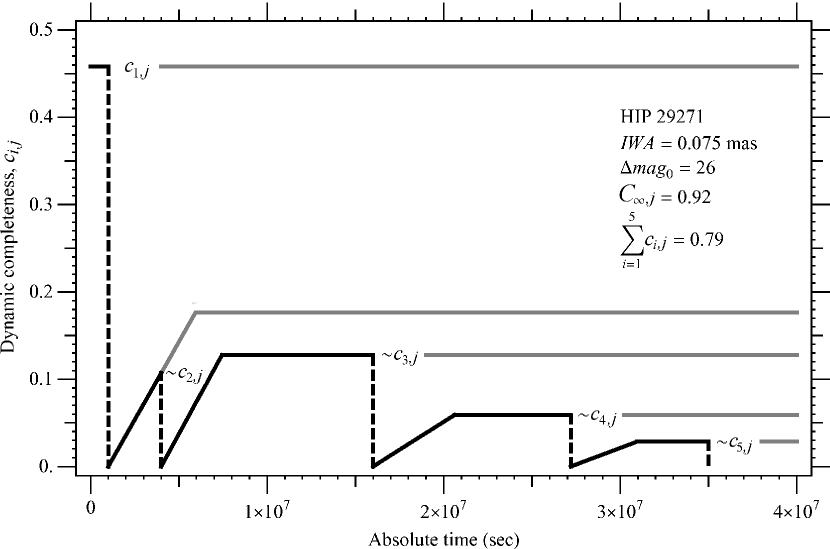
Figure 2: The dynamic completenesses of five hypothetical LSOs of HIP 29271 at $t=10^{6}$, $4\times 10^{6}$, $1.6\times 10^{7}$, $2.7\times 10^{7}$, and $3.5\times 10^{7}$ sec. The virgin completeness $c_{1,j}=0.46$ is an accurate value, independent of time and computed in advance of simulations, using Eq. 5. The symbols $c_{2-5,j}$ are preceded by tildes to indicate they are approximations. Such approximations would be used only in the selection process of a DRM, where it may be necessary to compute dynamic completeness for many stars on the fly. After the decision to observe a particular star, Eq. 5 would be used to produce an accurate value for the record. Note that as the number of LSOs of a star increases, the accumulate completeness converges on the ultimate completeness, $C_{\infty,j}$.

3 The Probability of a Discovery by the Next LSO, ${\cal P}$

After $i-1$ unproductive LSOs of star $j$, ($1-C_{i-1,j}$) is the fraction of all possible POIs that have not been ruled out and are still in play. The fraction of the remaining POIs that the next ($i^{\mathrm{th}}$) LSO at time $t$ would detect is

$${\cal K}_{i,j}(t)=\frac{c_{i,j}(t)}{(1-C_{i-1,j})}~{}.$$ (8)

The probability of a discovery on the next LSO of star $j$ is

$${\cal P}_{i,j}={\eta}^{\prime}_{j}{\cal K}_{i,j}(t)~{},$$ (9)

where ${\eta}^{\prime}_{j}$ is the Bayesian correction of the occurrence probability $\eta$. ${\eta}^{\prime}_{j}$ is the probability that star $j$ possesses a POI after taking into account the contrary evidence of $n_{j}$ previous unproductive LSOs with accumulated completeness $C_{i-1,j}$.

Bayes’s theorem states:

$${\eta}^{\prime}_{j}\equiv P({\cal H}|{\cal E})=\frac{P({\cal E}|{\cal H})P({\cal H})}{P({\cal E})}=\frac{(1-C_{i-1,j})\eta}{1-\eta C_{i-1,j}}~{},$$ (10)

where the hypothesis ${\cal H}$ is that star $j$ has a POI; the evidence ${\cal E}$ is the lack of a discovery so far; $P({\cal E}|{\cal H})=(1-C_{i-1,j})$ is the conditional probability of ${\cal E}$ if ${\cal H}$ is true; $P({\cal H})=\eta$ is the prior probability of ${\cal H}$; and the marginal probability of ${\cal E}$ is

$$P({\cal E}) = P({\cal E}|{\cal H})P({\cal H})+P({\cal E}|\overline{{\cal H}})P(\overline{{\cal H}})$$ (11)

$$= (1-C_{i-1,j})\eta+(1-\eta)=1-\eta C_{i-1,j}~{},$$

where $\overline{\cal H}$ is the hypothesis that star $j$ does not have a POI. [$P({\cal E}|\overline{{\cal H}})=1$ and $P(\overline{{\cal H}})=1-\eta$.]

The result for ${\cal P}_{i,j}$ is

$${\cal P}_{i,j}=\frac{\eta c_{i,j}(t)}{1-\eta C_{i-1,j}}~{}.$$ (12)

For the case of no prior searches ($i=1,\ C_{0,j}\equiv 0$), the probability of a discovery on the first search is $\eta c_{1,j}$, as expected.

We want to confirm numerically that Eq. 12 accurately estimates the probability of a discovery by the next LSO for random values of the parameters, for example, $\eta=0.272673$, $C_{1,j}=0.437671$, and $c_{2,j}=0.506385$, for which ${\cal P}_{2,j}=0.156789$. For this verification, we conduct $N_{\mathrm{obs}}=200,000$ independent LSOs, each involving $N_{0}=200,000$ possible POIs. Each LSO involves the following computational steps:

1. Randomly pick the serial number of the “real” POI: $n={\cal B}(\eta){\cal I}(1,N_{0})$, where ${\cal B}$ is a Bernoulli random deviate with probability $\eta$, which yields the value 0 or 1, and ${\cal I}$ is a uniform random deviate producing an integer in the range 1 to $N_{0}$. (If the serial number is zero, it means the “star” being observed does not have a POI.)

2. Perform a first LSO by selecting $N_{1}=\textsc{Round}(C_{1,j}N_{0})$ random integers in the range 1 to $N_{0}$, where the Round function yields the closest integer to the argument. If $n$ is one of these $N_{1}$ integers, then go back and repeat Steps 1 and 2, because we only want cases where the first LSO does not make a “discovery.”

3. Perform a second LSO by randomly selecting $N_{2}=\textsc{Round}(c_{2,j}N_{0})$ integers from the $N_{0}$–$N_{1}$ integers defined by excluding the $N_{1}$ integers in Step 2 from the set of all integers 1 to $N_{0}$. If $n$ is equal to one of these $N_{2}$ integers, then we have a discovery; otherwise, not.

4. Repeat Steps 1 to 3 $N_{\mathrm{obs}}$ times, and count the number of discoveries, $N_{\mathrm{disc}}$.

5. Compute the empirical probability, $N_{\mathrm{disc}}/N_{\mathrm{obs}}$, which was 0.156845, 0.157050, and 0.156695 in three runs we performed using the parameters above. These values compare well with the theoretical value, ${\cal P}_{2,j}$ and confirm Eq. 12. (As a benchmark, one run required 20,000 sec on a 3 GHz Intel Xenon processor running Mathematica 6.)

4 Applications of ${\cal P}$ to Observing Programs

Two applications of ${\cal P}$ and Eq. (12) must be sharply distinguished. The first application is in the scheduling algorithm for real or simulated observing programs, where we use the discovery rate,

$${\cal Z}_{i,j}=\frac{{\cal P}_{i,j}}{t_{\mathrm{exp}}+OH}~{},$$ (13)

as a merit function or science benefit/cost metric for optimizing the observing program for discovery. In this application, $\eta$ in Eq. (12) is $\eta_{\mathrm{ops}}$. (OH is any observational overhead time that will be charged to the program, such as for calibration or alignment.)

The second application of Eq. (12) is in estimating the probability distribution of discoveries for simulated observing programs, as discussed below. In this application, $\eta=\eta_{\mathrm{true}}$, where $\eta_{\mathrm{true}}$ is the “true” value. In this context, $\eta_{\mathrm{true}}$ is a control parameter. If $\eta_{\mathrm{ops}}\neq\eta_{\mathrm{true}}$, the number of planets discovered by an observing program may be less than optimal, because the scheduling algorithm may not always choose, as the next star to observe, the qualified star with the highest “true” value of the merit function.

In both applications of Eq. (12), $C_{i-1,j}$ is the accumulated completeness from all LSOs of star $j$ prior to the $i^{\mathrm{th}}$, each contribution computed as accurately as desired from Eq. (5).

4.1 Probability Distribution of the Number of Discoveries, pdf(m)

No matter what star $j$, nor what search $i$ of that star, the $k^{\mathrm{th}}$ LSO in the overall observing program discovers $u$ planetary systems, where $u\in\{0,1\}$ is a Bernoulli random variable with probability ${\cal P}_{k}$, as given in Eq. (12) using $\eta_{\mathrm{true}}$ and the indices $i$ and $j$ corresponding to the $k^{\mathrm{th}}$ LSO. [For each star ($j$), multiple visits ($i$) are possible, so both $i$ and $j$ define the $k^{\mathrm{th}}$ LSO.] The probability density function (pdf) of $u$ for the $k^{\mathrm{th}}$ LSO is

$$\textit{pdf}_{k}(u)=(1-{\cal P}_{k})\delta(u,0)+{\cal P}_{k}\delta(u,1)~{},$$ (14)

where $\delta(i,j)\equiv 1$ for $i=j$, and zero otherwise, is the Kronecker delta.

An entire observing program, consisting of $n_{\mathrm{total}}$ LSOs, where

$$n_{\mathrm{total}}=\sum\limits_{j=1}^{n_{\mathrm{stars}}}{n_{j}}~{},$$ (15)

where $n_{j}$ is the total number of LSOs of star $j$, and where $n_{\mathrm{stars}}$ is the total number of stars observed, discovers $m$ planets, where $m\in\{0,1,{\ldots}n_{\mathrm{total}}\}$ is the sum of $n_{\mathrm{total}}$ Bernoulli random variables, each with $\textit{pdf}_{k}$ given by Eq. (14). Therefore, the pdf of $m$ is the convolution ($\star$) of $\textit{pdf}_{k}$ for all $k$:

$$\textit{pdf}\,(m)=\textit{pdf}_{1}(u)\star\textit{pdf}_{2}(u)\star\ldots\star\textit{pdf}_{n_{\mathrm{total}}}(u)~{},$$ (16)

where each successive convolution has the form

$$(\textit{pdf}_{k}\star{\cal F})(n)\equiv(1-{\cal P}_{k}){\cal F}(n)+{\cal P}_{k}{\cal F}(n-1)~{}.$$ (17)

Equation (16) offers a practical advantage for estimating the outcome of a search program. Starting from a single simulated observing program, it allows us to estimate theoretically the pdf of the total number of discoveries. The alternative—running many full simulations to build up an empirical estimate of the pdf from the discovery results—is much less efficient.

4.2 Estimation of $\eta$

The pertinent record of a real or simulated observing program is a set of $n_{\mathrm{total}}$ data triplets re-indexed from $i$ (LSO) and $j$ (star) to $k$ (observation):

$$\left\{{c_{k},\ C_{k},\ u_{k}}\right\}\equiv\left\{{c_{i,j},\ C_{i-1,j},\ u_{i,j}}\right\}~{},$$ (18)

for $1\leq k\leq n_{\mathrm{total}}$, where $u_{i,j}=0$ or 1 is the number of discoveries by the $i^{\mathrm{th}}$ LSO of the $j^{\mathrm{th}}$ star. (If we assume that we stop searching after a discovery, $u_{i,j}=1$ for at most one value of $i$ for any $j$.)

The logarithmic likelihood function ${\cal L}$ is the logarithm of the probability of the set $\{u_{k}\}\equiv\{u_{i,j}\}$ as a function of $\eta$:

$${\cal L}(\{u_{k}\}|\eta)=\sum\limits_{k=1}^{n_{\mathrm{total}}}{\ln p_{u_{k}}}=\sum\limits_{k=1}^{n_{\mathrm{total}}}{\ln\left({\frac{c_{k}\eta}{1-C_{k}\eta}u_{k}+\left({1-\frac{c_{k}\eta}{1-C_{k}\eta}}\right)(1-u_{k})}\right)}~{}.$$ (19)

The maximum-likelihood estimate of the occurrence probability, $E(\eta)$, is the $\eta$-root of the equation:

$$\frac{\partial{\cal L}(\{u_{k}\}|\eta)}{\partial\eta}=0~{}.$$ (20)

The minimum variance bound (MVB) is the inverse of the Fisher information near $E(\eta)$:

$$\mathrm{MVB}\left(E(\eta)\right)=\left({\left.{-\frac{\partial^{2}{\cal L}(\{u_{k}\}|\eta)}{\partial\eta^{2}}}\right|_{\eta=E(\eta)}}\right)^{-1}~{}.$$ (21)

We want to confirm that Eqs. (19–21) accurately estimate $\eta$ and its variance. To that end, we performed a numerical experiment simulating 100,000 missions of 100 LSOs, according to the following steps.

1. Generated $n_{\mathrm{total}}=100$ random data triplets for the left side of Eq. (18) as follows:

   $$c = {\cal R}~{},$$ (22)

   $$C = (1-c){\cal R}~{},$$ (23)

   $$u = {\cal B}\left({\frac{\eta c}{1-\eta C}}\right)~{},$$ (24)

   where ${\cal R}$ is a uniform random deviate on the range 0–1, ${\cal B}(p)$ is a Bernoulli random deviate with probability $p$, and $\eta=0.10$.

2. Compute $E(\eta)$ and MVB($E(\eta)$) using Eqs. (19–21).

For the sample of 100,000 trials, we found

$$\langle E(\eta)\rangle=0.101~{},$$ (25)

$$\sigma_{\eta}=0.039~{},$$ (26)

and

$$\left\langle\sqrt{{\rm MVB}(E(\eta))}\right\rangle=0.042~{}.$$ (27)

Equation (25) is the mean value of $\eta$ found using Eq. (20) in the 100,000 simulated missions. Equation (26), the standard deviation of those values of $\eta$, is the empirical estimate of the scatter in $\eta$ determined by Eq. (20). The square of Eq. (26) is the empirical variance. The Cramér-Rao theoretical limit on the variance of any estimator of $\eta$ is the MVB given by Eq. (21). We computed the MVB for each simulated mission, and Eq. (27) gives the mean value of the square root of the MVB for the suite of 100,000 simulated missions—computed for direct comparison with the empirical value in Eq. (26).

These results illustrate that the maximum likelihood estimator accurately recovers $\eta$ from a record of the results of observing programs, and that the accuracy of this estimator appears to approach the Cramér-Rao limit ($\sigma^{2}\approx$ MVB). (This Monte Carlo experiment required 270 sec on 56 2.66 GHz Intel Xenon processors operating in parallel.)

5 Illustrative Design Reference Missions (DRMs)

The purpose of a design reference mission (DRM) is to gauge the science operations of a mission concept. To illustrate the new completeness methods introduced in this paper, we now describe a ministudy using simple DRMs to explore and measure of the power of the James Webb Space Telescope (JWST) to discover and characterize Earth-like extrasolar planets using a starshade to suppress scattered starlight (Cash et al., 2009; Soummer et al., 2009a). In this scenario, JWST and the starshade revolve in coordinated orbits around the second Earth-Sun Lagrange point, L2. The starshade operates on a $\sim$70,000 km sphere centered on JWST. In a 3-year planet-finding mission, we assume enough propulsion to slew the starshade 70 times to take up new positions between JWST and target stars. We want the DRMs to tell us about the science, for example how many discoveries to expect if we optimize the observing program, assuming $\eta_{\mathrm{true}}=\eta_{\mathrm{ops}}=0.3$, say.

Other DRM inputs include: a science strategy; a definition of POIs (same as Section 2.2, with $q$ depending on filter as given in Table 1); IWA = 0.085 arcsec, $\Delta\textit{mag}_{0}=26$, and pointing restrictions $\gamma_{1}=85^{\circ}$ (solar avoidance) and $\gamma_{2}=105^{\circ}$ (starshade bright-side avoidance); an input catalog of stars; exposure time calculators; typical overheads OH; and a merit function—in this case, the discovery rate ${\cal Z}$—which we use to select the next star to search.

The science strategy is simple: we perform an LSO, and if a likely POI is discovered, we immediately perform additional spectrophotometry to characterize the body. Such immediate follow-up reduces the risk of a newly discovered POI becoming undetectable before it can be characterized, and avoids the difficulty of trying to recover it with inadequate knowledge of its orbit (Brown, Shaklan, & Hunyadi, 2007). If we discover a POI, we cease further LSOs of that star. If we do not find one, we move the starshade to the next target star, but we return to a star already searched if and when it once again offers the highest value of ${\cal Z}$.

The LSO is a deep image using whichever NIRCam filter offers maximum ${\cal Z}$. We call this filter the preferred filter, and it varies from star to star. The possible filters are listed in Table 1.

After an LSO finds a potential POI, we obtain images through the four non-preferred NIRCam filters for that star, and take a low-resolution spectrum with NIRSpec. We use exposure time calculators for NIRCam and NIRSpec, based on parameters from the instrument teams, to achieve $S/N=5$ on a source of magnitude $\textit{mag}_{j}+\Delta\textit{mag}_{0}$ for the LSOs, and $\textit{mag}_{j}+\Delta\textit{mag}_{\mathrm{median}}$ for the follow-up filter photometry and spectroscopy, where $\textit{mag}_{j}$ is the apparent magnitude of star $j$, and $\Delta\textit{mag}_{\mathrm{median}}$ is the median magnitude difference between the star and the universe of possibly detected POIs for that star. (If $\Delta\textit{mag}_{\mathrm{median}}>\Delta\textit{mag}_{0}$, we use $\Delta\textit{mag}_{0}$.)

At this stage of the study we do not try to refine our understanding of the exposure time calculation beyond the current estimates by the instrument teams (Marsha Rieke et al. and Peter Jakobsen et al., private communication). We use standard parameters based on instrument requirements. There may be better observing modes for this particular application (e.g., involving detector sub-arrays).

We interpolate standard stellar magnitudes and zero points to the effective wavelengths of each NIRCam filter and the NIRSpec prism, starting from the VJHK magnitudes from NStED (nsted.ipac.caltech.edu/) and the VJHK zero points from Leinert et al. (1998). We used a near-infrared spectrum of Earth calculated by Sara Seager (private communication) to estimate the effective geometric albedo $q$ of Earth at the wavelengths and resolving powers of each instrument modes. These parameters are listed in Table 1.

As illustrated in Figure 3, each potential target star is continuously observable only for a limited period of time, once or twice a year, depending on its ecliptic latitude ($b$). The total time costs of observing a star—itemized in Table 2—must fit into a single observability period for that star. Some 26 of the 117 target stars Brown (2005) used in an earlier study of the coronagraphic Terrestrial Planet Finder (TPF–C) are qualified according to this criterion. These stars constitute the input catalog for these DRMs (Table 3).

Figure 3: The sphere of starshade operations, centered on JWST, shown here on the vernal equinox. Green: permitted pointings for $\gamma_{1}=85^{\circ}$ and $\gamma_{2}=105^{\circ}$. Red: forbidden pointings. As seen from above and as time passes, stars revolve on the starshade sphere around the $+\hat{z}$ axis (north ecliptic pole) in the clockwise direction. Depending on a star’s ecliptic latitude $b$, it may be observable for one or two periods per year, or for the entire year ($b>85^{\circ}$). Blue: a typical TPF-C target star from Brown (2005, HIP 92043, $b=+43.4^{\circ}$). Black: other TPF-C stars. Cyan: the Sun, which is fixed in this L2 coordinate system ($-\hat{x}$ toward the Sun, $+\hat{y}$ in the direction of the Earth’s orbital motion).

To determine the preferred filter for LSOs, we use Eq. (5) and the procedures of Section 2.2 to calculate virgin completeness $c_{1,j}$ for each of the 26 qualified stars using samples of $N_{0}=40,000$ POIs. We do this separately for each of the five filters, because of the dependence of $q$ on wavelength and resolving power. Next, we use Eqs. (12–13) to compute ${\cal P}_{1,j}$ and ${\cal Z}_{1,j}$, using OH = 10 hours as our estimate of the time cost of the fine alignment of the starshade, which we assume is incurred by each new observation with a different instrument, or of a different star. For each star $j$, we select the filter with the highest value of ${\cal Z}_{1,j}$ as the preferred filter for LSOs of that star (listed in Table 3).

Next, we determine the universe of possible LSOs. For the preferred filter only, we continue to compute $c_{i>1,j}$ using Eq. (5) until the sample of $N_{0}$ POIs is effectively exhausted. This yields 26 lists of dynamic completenesses, in sequence, one list for each of the 26 stars—some 2,075 values of $c_{i,j}$ in all. Again using Eqs. (12–13), we convert these lists of $c_{i,j}$ into a full list of possible LSOs in the form of vectors {HIP_k, $i_{k}$, ${\cal P}_{k}$, ${\cal Z}_{k}$}, where $1\leq k\leq 2075$ is the index for LSOs introduced in Section 4.1, and the items are the Hipparcos number of the star, the number of this visit to that star, and the discovery probability and rate for that visit.

At the start of a DRM, the prioritized observing program is the list of 2,075 LSO vectors sorted in descending order of ${\cal Z}_{k}$. (Table 4 lists the top 80 LSOs for the current illustration.) We expect to perform only 70 LSOs—but we do not know which ones. How far down the list a DRM reaches is determined by the random discoveries as the DRM unfolds. That is, we determine the outcome of each LSO in turn—discovery, yes or no, with possible follow-on observations and alternative time costs in Table 2—by interrogating a Bernoulli random deviate with probability ${\cal P}$, and interpreting “1” as a discovery and “0” as no discovery. Each discovery deletes from the observing program all the pending LSOs of a star—meaning those with $i$ greater than the visit number $i$ of the LSO that produced the discovery. These deletions promote the lower priority LSOs of other stars into higher positions on the list. To investigate this behavior and its ramifications, we conduct a Monte Carlo experiment of 500,000 DRMs.

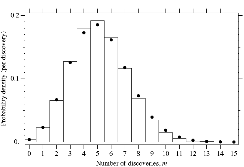
Figure 4: Comparison of the theoretical and empirical pdf($m$). Dots: the theoretical pdf estimated from the 70 values of ${\cal P}_{k}$ of the actual LSOs in the single example DRM in Table 4. Histogram: the empirical pdf from the actual results for $m$ in 500,000 DRMs. (The histogram has been normalized to 1.0.)

Table 4 provides an example DRM in the form of the LSOs actually executed in one DRM run, and the discoveries actually made—five in this case. We use it to illustrate the method of deriving the theoretical probability distribution of $m$ from the probabilities ${\cal P}_{k}$ of a single DRM. We collect the 70 values of ${\cal P}_{k_{\mathrm{DRM}}}$ for $1\leq k_{\mathrm{DRM}}\leq 70$ in Table 4 and follow the recipe in Section 4.1 to obtain the theoretical pdf($m$) represented by the dots in Figure 4. For comparison, the histogram in Figure 4 shows the empirical pdf($m$) based on the actual values of $m$ from 500,000 DRMs.

Table 5 compares the means, standard deviations, and standard deviations of the means—$\langle m\rangle$, $\sigma_{m}$, and $\sigma_{\langle m\rangle}$—for the results ensuing from Table 4, which encompass both the example DRM and the 500,000 DRMs computed from the same suite of potential or actual LSOs ($1\leq k\leq 2075$ or $1\leq k_{\mathrm{DRM}}\leq 70$). The highest precision is achieved by the mean of the 500,000 individual theoretical results for $\langle m\rangle$. We see that our new method produces accurate theoretical estimates of $\langle m\rangle$ and $\sigma_{m}$ from a single DRM and avoids the onerous alternative, which is to conduct a large number of DRMs to obtain empirical results.

The 500,000 DRMs ensuing from the prioritized LSOs in Table 4 offer additional insights into the science operations of the JWST starshade mission. The most likely number of unique stars searched is 23 (ranges 22–25). The median number of visits per star is 3. The total JWST observing time used by a DRM is $7.6\pm 1.3\times 10^{6}$ sec, and the total number of LSOs is 70 (here, this is the limiting parameter). Note that the total observing time corresponds to only $\sim$7% of the total JWST observing time. The most likely probability of zero discoveries is 0.004 (ranges 0.003 to 0.006).

Table 6 gives the data triplets defined in Eq. (18), which we use to estimate $\eta_{\mathrm{true}}=0.30\pm 0.12$, where the quoted error is the square root of the MVB.

A last note on this ministudy. We have not treated the recovery times of $c_{i,j}$ discussed in Section 2.3 because these example DRMs are “dilute,” meaning the LSOs account for only a small fraction of all the observations of JWST. In a “dense” DRM, with every LSO competing to be the next observation of the telescope, recovery time is important. Here, however, we can assume that a buffer of at least $\sim$10⁷ sec can conveniently pad the time between any two visits of the same star, which ensures adequate $c_{i,j}$ recovery.

6 Summary

In this paper, we have extended completeness-based metrics and algorithms for direct exoplanet searches to include multiple visits, estimating the probability distribution of search results, and estimating the occurrence rate of extrasolar planets. These extensions open the way for improved scheduling decisions, more realistic expectations for candidate instruments and missions, and enhanced science returns.

Preliminary DRMs for a starshade mission to enable Earth-like planet searches with JWST suggest a viable program for $<\!10^{7}$ sec of observing time. About five discoveries and spectral characterizations are expected if $\eta=0.3$. Soon, we hope, the Kepler mission will provide a first estimate of the true value of $\eta$.

Table 1: Spectrophotometric parameters for calculating completenesses and exposure times.

		Nominal $\lambda$	Resolving	Zero point	Earth geometric
Instrument	Mode	(nm)	power	(Jy)	albedo ($q$)
	F070W	0700	04	3043	0.232
	F115W	1150	04	1766	0.187
NIRCam	F140M	1400	10	1324	0.021
	F150W	1500	04	1188	0.103
	F162M	1625	10	1045	0.179
NIRSpec	prism	1150	31.7	1766	0.260

Note. — Zero points interpolated from values for VJHK filters (Leinert 1997). We adjusted the Earth’s effective albedo for prism spectroscopy at 1150 nm.

Table 2: Observing sequence and typical time costs for a single visit of the starshade to a target star.

Step	Activity	Observing time cost	Clock time cost
1	Final alignment of JWST, starshade, and target star	10 hours	10 hours
2	LSO through preferred NIRCam filter	$4.8\times 10^{4}$ sec	$4.8\times 10^{4}$ sec
3	Analyze data for discovery		7 days
4	Final alignment of JWST, starshade, and target star	10 hours	10 hours
5	Images through four non-preferred NIRCam filters	$1.4\times 10^{5}$ sec	$1.4\times 10^{5}$ sec
6	Analyze data to prepare for spectroscopy		7 days
7	Final alignment of JWST, starshade, and target star	10 hours	10 hours
8	Spectrum using NIRSpec	$1.9\times 10^{5}$ sec	$1.9\times 10^{5}$ sec
	Total with discovery	$4.9\times 10^{5}$ sec	$1.7\times 10^{6}$ sec
	Total without discovery	$8.4\times 10^{4}$ sec	$6.9\times 10^{5}$ sec

Note. — Overhead costs (1, 3, 4, 6, 7) are fixed. Exposure times (2, 5, 8) are median values for the 26 stars in the input catalog. With no discovery in step 3, only steps 1–3 are executed during a visit to a target star. With a discovery, all 8 steps are executed. During the analysis steps (3, 6), JWST conducts observations for other programs; only the starshade remains aligned with the target star for this program.

Table 3: The input catalog of target stars, ranked in descending order of the discovery rate on the first LSO (${\cal Z}_{1}$).

									Max
Disc.				Distance		LSO	LSO	Max	cont.
rate	HIP	Type	$L$	(pc)	$b(^{\circ})$	filter	$t_{\rm exp}$	time	obs.	$c_{1}$	$C_{\infty}$	${\cal P}_{1}$	${\cal Z}_{1}$
01	71681	K1 V	0.61	1.35	$-$43	F070W	3.2	6.12	6.38	0.8	1	0.24	$-$5.19
02	8102	G8 V	0.47	3.65	$-$25	F115W	4.03	6.13	6.29	0.76	1	0.23	$-$5.31
03	71683	G2 V	2.2	1.35	$-$43	F070W	2.43	6.12	6.38	0.55	1	0.17	$-$5.34
04	3821	G0 V	1.2	5.95	47	F115W	3.94	6.14	6.41	0.59	1	0.18	$-$5.4
05	99240	G6/8 IV	1.5	6.11	$-$45	F115W	4.12	6.16	6.4	0.56	1	0.17	$-$5.47
06	108870	K4/5 V	0.2	3.63	$-$41	F150W	4.48	6.13	6.37	0.65	1	0.19	$-$5.53
07	22449	F6 V	2.6	8.03	$-$15	F115W	3.88	6.15	6.26	0.39	0.96	0.12	$-$5.57
08	19849	K0/1 V	0.41	5.04	$-$28	F115W	4.69	6.16	6.3	0.64	1	0.19	$-$5.64
09	15510	G8 III	0.71	6.06	$-$58	F115W	4.68	6.18	6.53	0.63	1	0.19	$-$5.65
10	2021	G1 IV	3.9	7.47	$-$65	F070W	4.2	6.15	6.63	0.34	0.92	0.1	$-$5.7
11	27072	F6.5 V	2.3	8.97	$-$46	F115W	4.47	6.25	6.4	0.41	0.98	0.12	$-$5.73
12	1599	G0 V	1.2	8.59	$-$58	F115W	4.71	6.25	6.53	0.5	1	0.15	$-$5.76
13	64394	G0	1.3	9.15	33	F115W	4.81	6.3	6.32	0.47	1	0.14	$-$5.85
14	57757	F8	3.4	10.90	0.69	F115W	4.33	6.23	6.24	0.27	0.88	0.08	$-$5.85
15	12777	F8	2.2	11.20	32	F115W	4.64	6.31	6.32	0.36	0.99	0.11	$-$5.87
16	96100	G9 V	0.41	5.77	81	F115W	4.99	6.2	7.42	0.56	0.97	0.17	$-$5.9
17	105858	F7 V	1.4	9.22	$-$47	F115W	4.91	6.33	6.41	0.47	1	0.14	$-$5.92
18	73184	K4 V	0.26	5.91	$-$4.4	F150W	5.05	6.2	6.25	0.34	0.76	0.1	$-$6.17
19	70497	F8	3.9	14.60	60	F115W	4.75	6.41	6.56	0.17	0.81	0.051	$-$6.26
20	23693	F6/7 V	1.4	11.70	$-$79	F115W	5.18	6.53	7.42	0.33	0.91	0.098	$-$6.29
21	77952	F0 III/IV	9.6	12.30	$-$42	F070W	4.3	6.23	6.38	0.073	0.4	0.022	$-$6.41
22	29271	G6 V	0.83	10.20	$-$82	F115W	5.41	6.53	7.43	0.32	0.81	0.095	$-$6.49
23	114622	K3 V	0.28	6.53	55	F150W	5.34	6.27	6.49	0.27	0.68	0.081	$-$6.5
24	50954	F2/3 IV/V	5string	16.20	$-$68	F115W	4.98	6.57	6.7	0.11	0.68	0.032	$-$6.61
25	40702	F5 V	6.8	19.40	$-$75	F070W	5.29	6.66	7.41	0.076	0.61	0.023	$-$7.01
26	86614	F5	5.5	22string	84	F070W	5.6	6.93	7.46	0.048	0.67	0.014	$-$7.48

Note. — Times in log seconds. “Max time” is the time cost of the full observing sequence in Table 1. “Max cont. obs.” is the maximum continuous observing time for ecliptic latitude $b$ for $\gamma_{1}=85^{\circ}$ and $\gamma_{2}=105^{\circ}$. ${\cal P}_{1}$ is the probability of a discovery on the first LSO, from Eq. (12), and ${\cal Z}_{1}$ is ${\cal P}_{1}$ divided by the sum of LSO $t_{\mathrm{exp}}$ and 10 hours for alignment, from Eq. (13). The value of ${\cal Z}_{1}$ is given in log discoveries per sec.

Table 4: Record of a typical DRM.

$k$	$k_{\mathrm{DRM}}$	HIP	$i$	${\cal P}_{k}$	${\cal Z}_{k}$	Discovery	$|$	$k$	$k_{\mathrm{DRM}}$	HIP	$i$	${\cal P}_{k}$	${\cal Z}_{k}$	Discovery
1	01	71681	1	0.24	$-$5.19	no		41	37	57757	3	0.039	$-$6.17	no
2	02	8102	1	0.23	$-$5.31	yes		42	38	105858	2	0.075	$-$6.19	no
3	03	71683	1	0.17	$-$5.34	no		43	$\cdots$	71683	4	0.022	$-$6.22	$\cdots$
4	04	3821	1	0.18	$-$5.40	no		44	39	12777	3	0.046	$-$6.24	no
5	05	99240	1	0.17	$-$5.47	yes		45	40	2021	4	0.029	$-$6.26	no
6	06	108870	1	0.19	$-$5.53	no		46	41	70497	1	0.051	$-$6.26	no
7	07	22449	1	0.12	$-$5.57	no		47	42	23693	1	0.098	$-$6.29	no
8	08	19849	1	0.19	$-$5.64	no		48	43	57757	4	0.029	$-$6.30	no
9	09	15510	1	0.19	$-$5.65	no		49	44	1599	3	0.043	$-$6.31	no
10	10	71683	2	0.079	$-$5.66	yes		50	45	96100	2	0.065	$-$6.31	no
11	11	2021	1	0.10	$-$5.70	no		51	46	108870	3	0.032	$-$6.32	no
12	12	27072	1	0.12	$-$5.73	no		52	$\cdots$	8102	3	0.022	$-$6.32	$\cdots$
13	13	1599	1	0.15	$-$5.76	no		53	47	27072	4	0.030	$-$6.34	no
14	14	3821	2	0.077	$-$5.77	no		54	48	4394	3	0.045	$-$6.35	no
15	15	22449	2	0.070	$-$5.79	no		55	49	71681	3	0.017	$-$6.35	no
16	$\cdots$	99240	2	0.079	$-$5.79	$\cdots$		56	$\cdots$	99240	4	0.022	$-$6.35	$\cdots$
17	16	71681	2	0.054	$-$5.84	no		57	50	22449	5	0.019	$-$6.36	no
18	17	64394	1	0.14	$-$5.85	no		58	51	70497	2	0.040	$-$6.37	no
19	18	57757	1	0.080	$-$5.85	no		59	$\cdots$	3821	4	0.019	$-$6.37	$\cdots$
20	19	12777	1	0.11	$-$5.87	no		60	52	15510	3	0.035	$-$6.38	no
21	$\cdots$	8102	2	0.059	$-$5.90	$\cdots$		61	53	12777	4	0.033	$-$6.39	no
22	20	96100	1	0.17	$-$5.90	no		62	54	2021	5	0.020	$-$6.41	yes
23	21	2021	2	0.063	$-$5.91	no		63	55	77952	1	0.022	$-$6.41	no
24	22	105858	1	0.14	$-$5.92	no		64	56	105858	3	0.045	$-$6.42	no
25	23	27072	2	0.073	$-$5.96	no		65	57	19849	3	0.032	$-$6.42	no
26	$\cdots$	71683	3	0.040	$-$5.96	$\cdots$		66	58	57757	5	0.020	$-$6.45	no
27	24	22449	3	0.044	$-$6.00	no		67	59	70497	3	0.031	$-$6.48	no
28	25	108870	2	0.065	$-$6.01	no		68	60	29271	1	0.095	$-$6.49	no
29	26	57757	2	0.055	$-$6.02	no		69	61	73184	2	0.048	$-$6.49	no
30	27	1599	2	0.075	$-$6.06	no		70	62	22449	6	0.014	$-$6.49	no
31	28	12777	2	0.069	$-$6.07	no		71	$\cdots$	71683	5	0.012	$-$6.50	$\cdots$
32	29	15510	2	0.071	$-$6.07	no		72	63	23693	2	0.060	$-$6.50	no
33	30	3821	3	0.038	$-$6.08	yes		73	64	114622	1	0.081	$-$6.50	no
34	$\cdots$	99240	3	0.041	$-$6.08	$\cdots$		74	65	27072	5	0.021	$-$6.50	no
35	31	2021	3	0.042	$-$6.09	no		75	66	1599	4	0.026	$-$6.52	no
36	32	19849	2	0.068	$-$6.09	no		76	67	77952	2	0.017	$-$6.52	no
37	33	64394	2	0.074	$-$6.13	no		77	68	12777	5	0.022	$-$6.56	no
38	34	27072	3	0.047	$-$6.15	no		78	69	57757	6	0.016	$-$6.56	no
39	35	22449	4	0.030	$-$6.16	no		79	70	64394	4	0.028	$-$6.56	no
40	36	73184	1	0.10	$-$6.17	no		80	$\cdots$	2021	6	0.014	$-$6.57	$\cdots$

Note. — $k$: order of top 80 LSOs in terms of discovery rate ${\cal Z}$; $k_{\mathrm{DRM}}$: order of 70 LSOs executed in this example DRM; $i$: number of this LSO of this star; ${\cal P}_{k}$: probability of discovering a POI in this LSO; ${\cal Z}_{k}$: log discovery rate of this LSO; ellipses indicate that this LSO was not peformed in this DRM due to a previous discovery.

Table 5: DRM results for $\langle m\rangle$, $\sigma_{m}$, and $\sigma_{\langle m\rangle}$ for the expected number of POIs discovered.

	Empirical				Theoretical
	$\langle m\rangle$	$\sigma_{m}$	$\sigma_{\langle m\rangle}$		$\langle m\rangle$	$\sigma_{m}$	$\sigma_{\langle m\rangle}$
Example DRM	5string	$\cdots$	$\cdots$		5.210	2.15	$\cdots$
500,000 DRMs	5.132	2.06	0.003		5.129	0.09	0.0001

Note. — Empirical results are based on counting the number of discoveries in Monte Carlo experiments where discoveries were decided by Bernoulli random deviates. Theoretical results use the methods of Section 4.1 to estimate pdf($m$) from the individual LSO probabilities (${\cal P}_{k})$, and the results are—or are derived from—that distribution. (The highest precision is achieved by the mean of the 500,000 individual theoretical results for $\langle m\rangle$.)

Table 6: Data triplets for estimation of $\eta$ from results of the typical DRM.

$k$	$c_{k}$	$C_{k}$	$u_{k}$		$k$	$c_{k}$	$C_{k}$	$u_{k}$		$k$	$c_{k}$	$C_{k}$	$u_{k}$
1	0.8038	0	0		25	0.1759	0.6484	0		48	0.1203	0.6833	0
2	0.7574	0	1		26	0.1681	0.2672	0		49	0.04000	0.9398	0
3	0.5537	0	0		27	0.2123	0.5008	0		50	0.04858	0.7929	0
4	0.5950	0	0		28	0.2043	0.3599	0		51	0.1264	0.1697	0
5	0.5560	0	1		29	0.1932	0.6266	0		52	0.08750	0.8198	0
6	0.6484	0	0		30	0.09530	0.8049	1		53	0.08603	0.6926	0
7	0.3886	0	0		31	0.1171	0.5334	0		54	0.05295	0.7275	1
8	0.6446	0	0		32	0.1827	0.6446	0		55	0.07265	0	0
9	0.6266	0	0		33	0.2121	0.4711	0		56	0.1190	0.6811	0
10	0.2199	0.5537	1		34	0.1264	0.6184	0		57	0.07973	0.8273	0
11	0.3442	0	0		35	0.07820	0.7147	0		58	0.05505	0.6267	0
12	0.4061	0	0		36	0.3361	0	0		59	0.09337	0.2960	0
13	0.5008	0	0		37	0.1120	0.4353	0		60	0.3181	0	0
14	0.2099	0.5950	0		38	0.2154	0.4657	0		61	0.1448	0.3361	0
15	0.2067	0.3886	0		39	0.1284	0.5642	0		62	0.03500	0.8414	0
16	0.1360	0.8038	0		40	0.07705	0.6505	0		63	0.1806	0.3261	0
17	0.4711	0	0		41	0.1697	0	0		64	0.2701	0	0
18	0.2672	0	0		42	0.3261	0	0		65	0.05180	0.8227	0
19	0.3599	0	0		43	0.07945	0.5473	0		66	0.06625	0.8257	0
20	0.5590	0	0		44	0.1126	0.7131	0		67	0.05485	0.07265	0
21	0.1893	0.3442	0		45	0.1813	0.5590	0		68	0.05650	0.7786	0
22	0.4657	0	0		46	0.07942	0.8242	0		69	0.04180	0.6818	0
23	0.2123	0.4061	0		47	0.07785	0.7449	0		70	0.06988	0.8035	0
24	0.1193	0.5953	0

Note. — $k$ here is $k_{\mathrm{DRM}}$ in Table 4. ${\cal P}_{k}$ in Table 4 can be recovered from $c_{k}$ and $C_{k}$ here using Eqs. (12 & 18) and $\eta=\eta_{\mathrm{ops}}=0.3.$

References

- Agol (2007) Agol, E. 2007, MNRAS, 374, 1271
- Brown (2004) Brown, R. A. 2004, ApJ, 607, 1003
- Brown (2005) Brown, R. A. 2005, ApJ, 624, 1010
- Brown (2009a) Brown, R. A. 2009a, ApJ, 699, 711
- Brown (2009b) Brown, R. A. 2009b, ApJ, 702, 1237
- Brown, Shaklan, & Hunyadi (2007) Brown, R. A., Shaklan, S. B., & Hunyadi, S. L. 2007, JPL 07-02 7/07, Proc. TPF-C Workshop ( 9/28–29/2007), ed. W. A. Traub (Pasadena, CA: JPL), 53
- Cash et al. (2008) Cash, W., Oakley, P., Turnbull, M., Glassman, T., Lo, A., Polidan, R., Kilston, S., & Noecker, C. 2008, in Space Telescopes and Instrumentation 2008: Optical, Infrared, and Millimeter, eds. Oschmann, J. M., Jr., de Graauw, M. W. M., & MacEwen, H. A., Proceedings of the SPIE, Vol. 7010, pp. 70101Q–70101Q-9
- Cash et al. (2009) Cash, W., Spergel, D. N., Soummer, R., Mountain, M., Hartman, K., Polidan, R., Glassman, T., & Lo, A. 2009, The New Worlds Probe: A starshade with JWST. Request for Information to Astro2010: The Astronomy and Astrophysics Decadal Survey, June 2009; http://newworlds.colorado.edu/documents/Decadal/cash_jwststarshades_ppp.pdf
- Catanzarite et al. (2006) Catanzarite, J., Shao, M., Tanner, A., Unwin, S., & Yu, J. 2006, PASP, 118, 1319
- Guyon et al. (2008) Guyon, O., Angel, J. R. P., Backman, D., Belikov, R., Gavel, D., Giveon, A., Greene, T., Kasdin, J., Kasting, J., Levine, M., Marley, M., Meyer, M., Schneider, G., Serabyn, G., Shaklan, S., Shao, M., Tamura, M., Tenerelli, D., Traub, W., Trauger, J., Vanderbei, R., Woodruff, R. A., Woolf, N. J., & Wynn, J. 2008, in Space Telescopes and Instrumentation 2008: Optical, Infrared, and Millimeter, eds. Oschmann, J. M., Jr., de Graauw, M. W. M., & MacEwen, H. A., Proceedings of the SPIE, Vol. 7010, pp. 70101Y–70101Y-9
- Leinert et al. (1998) Leinert, Ch., Bowyer, S., Haikala, L. K., Hanner, M. S., Hauser, M. G., Levasseur-Regourd, A.-Ch., Mann, I., Mattila, K., Reach, W. T., Schlosser, W., Staude, H. J., Toller, G. N., Weiland, J. L., Weinberg, J. L., & Witt, A. N. 1998, A&AS, 127, 1
- Savransky, Kasdin, & Cady (2010) Savransky, D., Kasdin, N. J., & Cady, E. 2010, submitted to PASP; arXiv:0903.4915
- Soummer et al. (2009a) Soummer, R., Cash, W., Brown, R. A., Jordan, I., Roberge, A., Glassman, T., Lo, A., Seager, S., & Pueyo, L. 2009a, in Techniques and Instrumentation for Detection of Exoplanets IV, ed. Shaklan, S. B., Proceedings of the SPIE, Vol. 7440, pp. 74400A–74400A-15
- Soummer et al. (2009b) Soummer, R., Levine, M., & Exoplanet Forum Direct Optical Imaging Group 2009b, Exoplanet Community Report on Direct Optical Imaging, ch. 3; http://exep.jpl.nasa.gov/
- Spergel et al. (2009) Spergel, D. N., Kasdin, J., Belikov, R., Atcheson, P., Beasley, M., Calzetti, D., Cameron, B., Copi, C., Desch, S., Dressler, A., Ebbets, D., Egerman, R., Fullerton, A., Gallagher, J., Green, J., Guyon, O., Heap, S., Jansen, R., Jenkins, E., Kasting, J., Keski-Kuha, R., Kuchner, M., Lee, R., Lindler, D., Linfield, R., Lisman, D., Lyon, R., Malhotra, S., Mathews, G., McCaughrean, M., Mentzel, J., Mountain, M., Nikzad, S., O Connell, R., Oey, S., Padgett, D., Parvin, B., Procashka, J., Reeve, W., Reid, I. N., Rhoads, J., Roberge, A., Saif, B., Scowen, P., Seager, S., Seigmund, O., Sembach, K., Shaklan, S., Shull, M., & Soummer, R. 2009, in American Astronomical Society, AAS Meeting #213, Bulletin of the American Astronomical Society, Vol. 41, p. 362