Asymptotic study of subcritical graph classes

Abstract.

We present a unified general method for the asymptotic study of graphs from the so-called “subcritical” graph classes, which include the classes of cacti graphs, outerplanar graphs, and series-parallel graphs. This general method works both in the labelled and unlabelled framework. The main results concern the asymptotic enumeration and the limit laws of properties of random graphs chosen from subcritical classes. We show that the number $g_{n}/n!$ (resp. $g_{n}$) of labelled (resp. unlabelled) graphs on $n$ vertices from a subcritical graph class ${\mathcal{G}}=\cup_{n}{\mathcal{G}_{n}}$ satisfies asymptotically the universal behaviour

$$g_{n}\ \!=\ \!c\ \!n^{-5/2}\ \!\gamma^{n}\ \!(1+o(1))$$

for computable constants $c,\gamma$, e.g. $\gamma\approx 9.38527$ for unlabelled series-parallel graphs, and that the number of vertices of degree $k$ ($k$ fixed) in a graph chosen uniformly at random from $\mathcal{G}_{n}$, converges (after rescaling) to a normal law as $n\to\infty$.

1. Introduction

Several enumeration problems on classes of labelled planar structures, e.g. labelled planar graphs, were solved recently [5, 6, 20]. These results were successfully used for efficient random generators for labelled planar graphs [17], based on Boltzmann samplers [14]. In contrast, less is known about enumerative results on classes of unlabelled planar structures: the only classes treated so far are forests [25] and more recently outerplanar graphs [4].

In this paper we present a general framework to enumerate in a unified way a wide variety of labelled and unlabelled classes of graphs. Our main contribution is a universal method for rich classes of unlabelled graphs, the so-called “subcritical” classes of graphs, which is established through the novel singularity analysis of counting series and yields asymptotic estimates and limit laws for various graph parameters. In order to make this method more accessible and transparent, we include a brief analysis of the corresponding labelled classes, which was already carried out in [21].

Another main contribution is asymptotic estimates and limit laws for various graph parameters of unlabelled series-parallel graphs. We study the class of unlabelled series-parallel graphs, firstly as an important subclass of planar graphs whose asymptotic study has not been carried out so far and therefore it is interesting in its own right, and secondly as a concrete prototype-example to illustrate how our general method is applied. A graph is series-parallel (SP-graphs for conciseness) if its $2$-connected components are obtained from a single edge by recursive subdivision of edges (series operation) and duplication of edges (parallel operation). Equivalently, SP-graphs can be defined in terms of minors as graphs which exclude $K_{4}$ as a minor. Finally, a graph is series-parallel if and only if its tree-width is at most $2$. Applying our general method, we show that the number ${g}_{n}$ of unlabelled SP-graphs on $n$ vertices is asymptotically of the form

$${g}_{n}\ \!=\ \!c\ \!n^{-5/2}\ \!\rho^{-n}\ \!(1+o(1)),$$

where $\rho\approx 0.10655$. Let ${G}_{n}$ be a graph chosen uniformly at random among all unlabelled SP-graphs on $n$ vertices. The random variable $X_{n}$ counting the number of edges (blocks, or cut-vertices) in ${G}_{n}$ features a central limit law

$$\frac{X_{n}-\mathbb{E}\,X_{n}}{\sqrt{\mathbb{V}{\mathrm{ar}}\,X_{n}}}\to N(0,1),$$

where $\mathbb{E}\,X_{n}=\mu n+O(1)$ and $\mathbb{V}{\mathrm{ar}}\,X_{n}=\sigma^{2}n+O(1)$ for computable constants $\mu$ and $\sigma^{2}$. In addition, the random variable $X_{n}^{k}$ counting the number of vertices of degree $k$ (for $k$ fixed) in ${G}_{n}$ satisfies a central limit law with mean $\mathbb{E}\,X_{n}^{k}=\mu_{k}n+O(1)$ and variance $\mathbb{V}{\mathrm{ar}}\,X_{n}^{k}=\sigma_{k}^{2}n+O(1)$ where $\mu_{k}$ and $\sigma_{k}^{2}$ are computable constants. We also present a simple and general condition assuring $\sigma^{2}>0$, which holds in a wide variety of graph families.

Furthermore we show that the same subexponential term $n^{-5/2}$ appears in other classes of graphs (in both labelled and unlabelled cases), which is, roughly speaking, inherited from a tree-like nature. This behaviour appears as a consequence of a subcritical composition scheme which appears in the specification of the counting series associated to connected graphs of the class. Such classes of graphs arising from subcritical composition scheme are called subcritical classes of graphs, whose formal definition is rather technical and therefore will be suspended to Sections 4 and 5.

We consider block-stable classes of graphs: we say a class $\mathcal{G}$ of graphs block-stable if and only if for each graph $G\in\mathcal{G}$, each of its $2$-connected components (also called blocks) belongs to $\mathcal{G}$. The class of cacti graphs, the class of outerplanar graphs, the class of SP-graphs, and other classes of graphs defined in terms of a class of $2$-connected components are block-stable. Additionally, we consider classes of graphs which are defined by a finite set of $3$-connected graphs. Observe that SP-graphs can be seen as graphs without 3-connected components. We show that the classes of cacti graphs, outerplanar graphs, and SP-graphs, are subcritical and prove that the asymptotic estimates and limit laws for graph parameters of subcritical classes of graphs follow the same asymptotic pattern and limit laws as the class of SP-graphs.

The asymptotic study of subcritical classes of graphs consists of two steps: formal and analytic steps. The formal step consists in translating Tutte’s seminal ideas on decomposing graphs into components of higher connectivity [7, 30, 31] in terms of the decomposition grammar, which is comparable to the ones introduced in [8] (see also [19]). This decomposition grammar translates combinatorial conditions into functional equations satisfied by the counting series of various classes of graphs. These counting series depend on the connectivity degree and the way how the graphs are rooted. In the analytic step, we extract singular expansions of the counting series from the systems of functional equations. The main ingredient in this step is from [10], in which precise singular expansions are deduced for very general systems of functional equations. Finally, we derive asymptotic formulas from these singular expansions by extracting coefficients, based on the transfer theorems of singularity analysis [15, 16].

We also study natural parameters on a uniform random graph on $n$ vertices chosen from a subcritical class, such as the number of edges, the number of blocks and the number of cut-vertices. These parameters satisfy normal limit laws, which come from the additivity behaviour of these parameters. We compute their expectation and variance, which characterise completely their limit distribution. These parameters were studied in [21] for various labelled classes of graphs. In this paper we rediscover these results for labelled case and obtain new results for unlabelled case. Finally, applying the general techniques for systems of functional equations we deduce the limit law for the degree distribution of a graph chosen uniformly at random among all the graphs on $n$ vertices, by analysing in a unified way both labelled and unlabelled subcritical classes. The present work complement the work [3, 12, 13] for related problems on labelled graphs. Other non-additive parameters, such as the size of the largest block are not treated here. This parameter was studied in the labelled framework in [21] and [26]. In the latter, the theory of Boltzmann samplers is applied.

Outline of the paper. The paper is organised as follows. In Section 2 we introduce the notation and the terminology used in this paper. All the analytic machinery needed in order to deal with systems of functional equations, extraction of coefficients and limit laws is introduced in Section 3. In this section, we adapt the results from [10] to our context and recall the transfer theorems of singularity analysis from [16] and other key results necessary to derive limit laws for graph parameters. We also introduce a novel result which assures the positivity of the variance under certain easy conditions. In Section 4 we obtain general results for the enumeration of labelled subcritical graph classes. These results are generalised to unlabelled subcritical graph classes in Section 5. These enumerative results we obtain are consequences of the general framework presented in Section 3. Concrete examples are studied in Section 6. This section includes the analysis of unlabelled cacti graphs, unlabelled outerplanar graphs, and unlabelled SP-graphs. We also obtain general enumerative results for classes of graphs defined by a finite set of $3$-connected graphs. Limit laws are studied in Section 7. All parameters studied in this section give rise to normal distributed random variables, independently of the class (in either labelled or unlabelled setting). The degree distribution, a technically more involved and interesting parameter, is studied in Section 8. Finally, the constant growth for unlabelled SP-graphs is computed in Section 9, using a numerical method.

2. Graph classes, block-decomposition, and counting

2.1. Combinatorial classes and counting series

As described in [2, 16], a labelled combinatorial class is a set $\mathcal{G}=\cup_{n\geq 0}\,\mathcal{G}_{n}$ of objects such that $\mathcal{G}_{n}$ is finite for $n\geq 0$. Each object $g$ in $\mathcal{G}_{n}$ has $n$ labelled “atoms”(e.g., vertices of a graph) carrying distinct labels in $\{1,\dots,n\}$ and $n$ is called the size of $g$. Two objects of $\mathcal{G}$ (of the same size $n$) are called isomorphic if one is defined from the other by relabelling. It is always assumed that a combinatorial class is stable under relabelling, e.g., for a graph class $\mathcal{G}$ we assume that a graph $g$ is in $\mathcal{G}$ if and only if all graphs isomorphic to $g$ are also in $\mathcal{G}$. This way the symmetric group $\mathfrak{S}_{n}$ acts on $\mathcal{G}_{n}$: for $\sigma\in\mathfrak{S}_{n}$ and $g\in\mathcal{G}_{n}$, $\sigma\cdot g$ has the same vertex and edge set as $g$, but each label $i$ in $g$ is replaced by $\sigma^{-1}(i)$ in $\sigma\cdot g$ and we write $\sigma\cdot g\equiv g$. The set of objects of $\mathcal{G}_{n}$ considered up to isomorphism is denoted by $\widetilde{\mathcal{G}}_{n}$ (in other words $\widetilde{\mathcal{G}}_{n}=\mathcal{G}_{n}/\mathfrak{S}_{n}$), and the combinatorial class $\widetilde{\mathcal{G}}:=\cup_{n}\,\widetilde{\mathcal{G}}_{n}$ is called the unlabelled combinatorial class associated with $\mathcal{G}$. For counting purpose one classically considers the exponential generating function (shortly the EGF) in the labelled setting:

$$\mathcal{G}(z):=\sum\nolimits_{n\geq 0}\frac{1}{n!}|\mathcal{G}_{n}|z^{n},$$

and the ordinary generating function (OGF) in the unlabelled setting:

$$\widetilde{\mathcal{G}}(z):=\sum\nolimits_{n\geq 0}|\widetilde{\mathcal{G}}_{n}|z^{n}.$$

For unlabelled enumeration, it proves convenient to consider a refinement of the OGF, called the cycle-index sum, a series in infinitely many variables $s_{1},s_{2},\ldots$ defined as

$$Z_{\mathcal{G}}(s_{1},s_{2},\ldots):=\sum\nolimits_{n\geq 0}\frac{1}{n!}\sum_{\begin{subarray}{c}(\sigma,g)\in\mathfrak{S}_{n}\times\mathcal{G}_{n}\\ \sigma\cdot g=g\end{subarray}}w_{\sigma},$$

where $w_{\sigma}:=s_{1}^{c_{1}}s_{2}^{c_{2}}\cdots s_{n}^{c_{n}}$ is the weight-monomial of a permutation $\sigma$ of cycle type $1^{c_{1}}2^{c_{2}}\cdots n^{c_{n}}$ (that is, $c_{i}$ cycles of length $i$ for $i=1,\dots,n$). The OGF is recovered from a specialisation of the cycle index sum [22] by replacing $s_{i}$ by $z^{i}$ for each $i\geq 1$:

$$\widetilde{\mathcal{G}}(z)=Z_{\mathcal{G}}(z,z^{2},z^{3},\ldots).$$

We will consider classes of graphs of various types depending on whether one marks vertices or not. All graphs are assumed to be simple (no loops nor multiple edges) and are labelled at vertices. A (vertex-)rooted graph is a graph with a distinguished (labelled) vertex. A derived graph or pointed graph is a graph where one vertex is distinguished but not labelled (the other $n-1$ vertices have distinct labels in $\{1,\dots,n-1\}$). Isomorphisms between two pointed graphs (or between two derived graphs) have to respect the distinguished vertex.

Given a graph class $\mathcal{G}$, the rooted class $\mathcal{G}^{\bullet}$ is the class of rooted graphs from $\mathcal{G}$, and the derived class $\mathcal{G}^{\prime}$ is the class of derived graphs from $\mathcal{G}$; since $|\mathcal{G}^{\prime}_{n-1}|=n|\mathcal{G}_{n}|$ and $|\mathcal{G}^{\bullet}_{n}|=n|\mathcal{G}_{n}|$, we have respectively $\mathcal{G}^{\prime}(z)=\frac{\mathrm{d}}{\mathrm{d}z}\mathcal{G}(z)$ and $\mathcal{G}^{\bullet}(z)=z\mathcal{G}^{\prime}(z)$.

2.2. Block-decomposition of a graph

For $k\geq 0$, a graph is $k$-connected if one needs to delete at least $k$ vertices to disconnect it. Obviously, a graph $G$ is a set of its connected components. For the decomposition from connected graphs into 2-connected graphs we use the block structure of a connected graph. A block of a graph $G$ is a maximal 2-connected induced subgraph of $G$. We say a vertex of $G$ is incident to a block $B$ of $G$ if it belongs to $B$. The block structure of $G$ yields a bipartite tree with the vertex set consisting of two types of nodes, i.e. cut-vertices and blocks of $G$, and the edge set describing the incidences between the cut-vertices and blocks of $G$. This suggests a natural decomposition of connected graphs into 2-connected graphs and this holds also for rooted graphs. The root-vertex $v$ of a rooted graph $G$ is incident to a set of blocks and to each non-root vertex on these blocks is attached a rooted connected graph. In other words, a rooted connected graph rooted at $v$ is uniquely obtained as follows: take a set of derived 2-connected graphs and merge them at their pointed (distinguished but not labelled) vertices so that $v$ is incident to these derived 2-connected graphs, then replace each non-root vertex $w$ in these blocks by a rooted connected graph rooted at $w$ (which is allowed to consist of a single vertex and in this case it has no effect).

Through the entire paper, given a class of graphs $\mathcal{G}$, we denote by $\mathcal{C}$ (resp. $\mathcal{B}$) the subfamily of connected (resp. $2$-connected) graphs in $\mathcal{G}$. In the language of symbolic combinatorics from [2, 16], the block-decomposition described above translates into the fundamental equations:

(1) $$\mathcal{G}=\mathrm{Set}(\mathcal{C}),$$

(2) $$\mathcal{C}^{\bullet}=\mathcal{Z}\cdot\mathrm{Set}(\mathcal{B}^{\prime}\circ\mathcal{C}^{\bullet}),$$

where the factor $\mathcal{Z}$ in the last equation takes account of the root vertex (which is distinguished and labelled), the symbol $\cdot$ denotes the partitional product on combinatorial classes, and the symbol $\circ$ denotes substitution at an atom (see [2] for definitions). As shown in Table 1, there is a well-known dictionary [2, 16], both in the labelled and in the unlabelled setting, that translates equations relating combinatorial classes into equations relating the associated counting series.

Construction	Class	Labelled setting	Unlabelled setting
Sum	$\mathcal{C}=\mathcal{A}+\mathcal{B}$	$\mathcal{C}(z)=\mathcal{A}(z)+\mathcal{B}(z)$	$\widetilde{\mathcal{C}}(z)=\widetilde{\mathcal{A}}(z)+\widetilde{\mathcal{B}}(z)$$\widetilde{\mathcal{C}^{\mathcal{C}}}$
Product	$\mathcal{C}=\mathcal{A}\cdot\mathcal{B}$	$\mathcal{C}(z)=\mathcal{A}(z)\cdot\mathcal{B}(z)$	$\widetilde{\mathcal{C}}(z)=\widetilde{\mathcal{A}}(z)\cdot\widetilde{\mathcal{B}}(z)$
Set	$\mathcal{C}=\mathrm{Set}(\mathcal{B})$	$\mathcal{C}(z)=\exp(\mathcal{B}(z))$	$\widetilde{\mathcal{C}}(z)=\exp\big{(}\sum_{i\geq 1}\tfrac{1}{i}\widetilde{\mathcal{B}}(z^{i})$)
Substitution	$\mathcal{C}=\mathcal{A}\circ\mathcal{B}$	$\mathcal{C}(z)=\mathcal{A}(\mathcal{B}(z))$	$\widetilde{\mathcal{C}}(z)=Z_{\mathcal{A}}(\widetilde{\mathcal{B}}(z),\widetilde{\mathcal{B}}(z^{2}),\ldots)$

Table 1. The dictionary that translates combinatorial constructions into operations on counting series.

A graph class $\mathcal{G}$ is called block-stable if it contains the link-graph $\ell$, which is a graph with one edge together with its two (labelled) end vertices, and satisfies the property that a graph $G$ belongs to $\mathcal{G}$ if and only if all the blocks of $G$ belong to $\mathcal{G}$. Block-stable classes include classes of graph specified by a finite list of forbidden minors that are all 2-connected, for instance, planar graphs ($\mathrm{Forbid}(K_{5},K_{3,3})$), series-parallel graphs ($\mathrm{Forbid}(K_{4})$), and outerplanar graphs ($\mathrm{Forbid}(K_{4},K_{3,2})$). For a block-stable graph class, (1) and (2) translates into equations of EGFs in the labelled setting:

$$\mathcal{G}(z)=\exp(\mathcal{C}(z)),$$

$$\mathcal{C}^{\bullet}(z)=z\exp(\mathcal{B}^{\prime}(\mathcal{C}^{\bullet}(z))),$$

and into equations of OGFs in the unlabelled setting:

$$\widetilde{\mathcal{G}}(z)=\exp\left(\sum\nolimits_{i\geq 1}\tfrac{1}{i}\widetilde{\mathcal{C}}(z^{i})\right),$$

$$\widetilde{\mathcal{C}^{\bullet}}(z)=z\exp\left(\sum\nolimits_{i\geq 1}\tfrac{1}{i}Z_{\mathcal{B}^{\prime}}(\widetilde{\mathcal{C}^{\bullet}}(z^{i}),\widetilde{\mathcal{C}^{\bullet}}(z^{2i}),\widetilde{\mathcal{C}^{\bullet}}(z^{3i}),\ldots)\right).$$

A refined version of the last equation will turn out to be useful later, which expresses (2) in terms of the cycle index sum:

(3) $$Z_{\mathcal{C}^{\bullet}}(s_{1},s_{2},\ldots)=s_{1}\exp\left(\sum\nolimits_{i\geq 1}\tfrac{1}{i}Z_{\mathcal{B}^{\prime}}(Z_{\mathcal{C}^{\bullet}}(s_{i},s_{2i},\ldots),Z_{\mathcal{C}^{\bullet}}(s_{2i},s_{4i},\ldots),\ldots)\right).$$

With these systems of equations of EGFs, OGFs and the cycle index sum, we will perform singularity analysis under certain general conditions – so-called “subcriticallity” conditions – in order to get asymptotic results (asymptotic enumeration and limit laws for graph parameters). The tools for singularity analysis are described in the next section.

3. Tools for the asymptotic analysis

The purpose of this section is to collect several facts on solutions of functional equations. Most of the following properties (and proofs) can be found in [11, 16], which serve as general references for this subject. For our purposes we, however, need to adjust several points with additional properties.

3.1. Singular expansions of multivariate series

We consider a power series of the form $y=y(z,v_{1},\ldots,v_{k})$ in general with nonnegative coefficients, where $z$ is singled out as the primary variable and $v_{1},\ldots,v_{k}$ are secondary variables (possibly there is none). From now on we use the abbreviation $\mathbf{v}$ for $(v_{1},\ldots,v_{k})$. A valuation $\mathbf{v}_{0}$ of $\mathbf{v}$ is called admissible if all components of $\mathbf{v}_{0}$ are positive and if $y(z,\mathbf{v}_{0})$ is a valid power series in $z$, i.e., $[z^{n}]y(z,\mathbf{v}_{0})<\infty$ for each $n\geq 0$.

Consider a fixed positive valuation $(z_{0},\mathbf{v}_{0})$ of $(z,\mathbf{v})$. Then $y$ is said to have a square-root expansion around $(z_{0},\mathbf{v}_{0})$ if $\mathbf{v}_{0}$ is an admissible valuation, $z_{0}$ is the radius of convergence of $y(z,\mathbf{v}_{0})$, and the representation

$$y(z,\mathbf{v})=a(z,\mathbf{v})-b(z,\mathbf{v})\sqrt{1-z/\rho(\mathbf{v})}$$

holds in a neighbourhood of $(z_{0},\mathbf{v}_{0})$ (except in the part where $1-z/\rho(\mathbf{v})\in\mathbb{R}^{-}$), where the functions $a(z,\mathbf{v})$ and $b(z,\mathbf{v})$ are analytic at $(z_{0},\mathbf{v}_{0})$, $b(z_{0},\mathbf{v}_{0})>0$, $\rho(\mathbf{v})$ is analytic at $\mathbf{v}_{0}$, and $\rho(\mathbf{v}_{0})=z_{0}$. The function $\rho(\mathbf{v})$ in the expansion is called the singularity function of $y$ relative to $z$.

Moreover, we will be particularly interested in functions $y(z,\mathbf{v})$ with such a singular behaviour, where $\rho(\mathbf{v})$ is the only singularity on the circle $|z|=|\rho(\mathbf{v})|$ (if $\mathbf{v}$ varies in a suitable neighbourhood of $\mathbf{v}_{0}$) and $y(z,\mathbf{v})$ can be analytically continued to the region $\{z\in\mathbb{C}:|z|<|\rho(\mathbf{v})|+\epsilon,\ 1-z/\rho(\mathbf{v})\not\in\mathbb{R}^{-}\}$ (for some $\epsilon>0$ that is uniform in this neighbourhood of $\mathbf{v}_{0}$). In this case one can use an asymptotic transfer principle by Flajolet and Odlyzko [15] (see also Section 3.3) to obtain asymptotics for the coefficient $[z^{n}]\,y(z,\mathbf{v})$ of the form

$$[z^{n}]\,y(z,\mathbf{v})=\frac{b(\rho(\mathbf{v}),\mathbf{v})}{2\sqrt{\pi}}\,n^{-3/2}\,\rho(\mathbf{v})^{-n}\,\left(1+O\left(n^{-1}\right)\right).$$

Similarly, $y$ is said to have a singular expansion of order $3/2$ at $(z_{0},\mathbf{v}_{0})$ if the expansion is of the form

$$y(z,\mathbf{v})=a(z,\mathbf{v})+b(z,\mathbf{v})\cdot(1-z/\rho(\mathbf{v}))^{3/2},$$

with otherwise the same conditions as for square-root expansions.

It is not difficult to show that if a function $y(z,\mathbf{v})$ admits a square-root expansion around $(z_{0},\mathbf{v}_{0})$, then the function $\int_{0}^{z}\,y(x,\mathbf{v})\,\mathrm{d}x$ admits a singular expansion of order $3/2$ at $(z_{0},\mathbf{v}_{0})$ (see [13]).

3.2. Singularity analysis of systems of functional equations

Consider a vector $\mathbf{y}=(y_{1},\ldots,y_{r})$ of formal power series in the formal variables $z,\mathbf{v}$, with $\mathbf{v}=(v_{1},\ldots,v_{k})$ which is a solution of an equation-system of the form

$$\mathrm{(E)}:\qquad\mathbf{y}=\mathbf{F}(\mathbf{y};z,\mathbf{v}),$$

where $\mathbf{F}(\mathbf{y};z,\mathbf{v})=(F_{1}(\mathbf{y};z,\mathbf{v}),\ldots,F_{r}(\mathbf{y};z,\mathbf{v}))$ are power series with nonnegative coefficients. In order to avoid trivial situations as in equations like $y=zy^{2}$, where $y(z)=0$ is the only solution, we will assume that $\mathbf{y}={\bf 0}$ is not a solution. We call such a system positive system.

The Jacobian matrix $\mathbf{Jac}_{\textbf{F}}$ of the system is the $r\times r$ matrix whose $(i,j)$-coefficient is $\partial F_{j}/\partial y_{i}$. The singularity equation associated with $\mathrm{(E)}$ is

$$\mathrm{(S)}:\qquad 0=\mathrm{Det}\left(\mathbf{I_{r}}-\mathbf{Jac}_{\textbf{F}}\right),$$

where $\mathbf{I_{r}}$ is the $r\times r$ identity matrix. The singularity system of ($\mathrm{E}$) is the system $\{\mathrm{(E)},\ \mathrm{(S)}\}$, which has $r+1$ equations (the first $k$ ones for ($\mathrm{E}$), the last one for ($\mathrm{S}$)).

The dependency graph of $\mathbf{F}$ is the directed graph on $V=\{1,\ldots,r\}$ such that there is an edge from $i$ to $j$ if and only if the $j$th component $F_{j}$ of $\mathbf{F}$ really involves $y_{i}$, that is, the power series $\partial F_{j}/\partial y_{i}$ is not $0$. The system $\mathrm{(E)}$ is called strongly recursive if the dependency graph of $\mathbf{F}$ is strongly connected (which means that every pair of vertices is linked by a directed path).

Informally this condition says that no subsystem of $\mathrm{(E)}$ can be solved prior to the whole system of equations. An equivalent condition is that the corresponding adjacency matrix and, thus, the Jacobian matrix $\mathbf{Jac}_{\textbf{F}}$ is irreducible. The most important property of irreducible matrices ${\bf A}$ with non-negative entries is the Perron-Frobenius Theorem (see [24]) saying that there is a unique positive and simple eigenvalue $\lambda_{max}=\lambda_{max}({\bf A})$ with the property that all other eigenvalues $\lambda$ satisfy $|\lambda|\leq\lambda_{max}$. This unique positive eigenvalue is a strictly increasing function of the entries of the non-negative matrix. More precisely, if ${\bf A}=(a_{ij})$ and ${\bf A}^{\prime}=(a_{ij}^{\prime})$ are different irreducible non-negative matrices with $a_{ij}\leq a_{ij}^{\prime}$ (for all $i,j$) then $\lambda_{max}({\bf A})\leq\lambda_{max}({\bf A}^{\prime})$. Moreover, every principal submatrix has a smaller dominant eigenvalue.

Consider an admissible valuation $\mathbf{v}_{0}$ of $\mathbf{v}$ and assume that the radius of convergence $z_{0}$ of $z\to y_{1}(z,\mathbf{v}_{0})$ is finite and strictly positive. If the system $\mathrm{(E)}$ is strongly recursive then it is easily shown that, for each $i\in\{1,\ldots,r\}$, $z_{0}$ is the radius of convergence of $y_{i}$ (due to the dependency graph being strongly connected) and $y_{i}(z,\mathbf{v}_{0})$ converges to a finite constant $\tau_{i}>0$ as $z\to z_{0}$ (due to the fact that $\mathbf{F}$ is nonlinear according to $\mathbf{y}$).

Note also that $\mathrm{(S)}$ says that $\lambda=1$ is an eigenvalue of $\mathbf{Jac}_{\textbf{F}}$. We observe that if $\mathbf{y}=\mathbf{y}(z,\mathbf{v}_{0})$ is an analytic solution of a strongly recursive system $\mathrm{(E)}$ that is singular at $z=z_{0}$ and $\mathbf{y}_{0}=\mathbf{y}(z_{0},\mathbf{v}_{0})$ is a finite vector, then $\mathrm{(S)}$ is satisfied for $(y;z,\mathbf{v})=(y_{0};z_{0},\mathbf{v}_{0})$ provided that $(y_{0};z_{0},\mathbf{v}_{0})$ is an inner point of the region of convergence of $\mathbf{F}$. (This explains the term singularity system.) However, in order to obtain the radius of convergence (in positive and analytically well-founded systems) we will need the condition that $\lambda_{max}(\mathbf{Jac}_{\textbf{F}})=1$ (see [1]).

Definition 1.

A system $\mathrm{(E)}$ is called analytically well-founded at a fixed positive valuation $\mathbf{v}_{0}$ if the following conditions are satisfied:

1. The valuation $\mathbf{v}_{0}$ is admissible for the system of power series $\mathbf{F}(\mathbf{y};z,\mathbf{v}_{0})$, we have $[\mathbf{y}^{\bf m}z^{n}]\,F_{i}(\mathbf{y};z,\mathbf{v}_{0})\geq 0$ for all $i$, and $[z^{n}]\mathbf{F}({\bf 0};z,\mathbf{v}_{0})\neq{\bf 0}$.

2. The function $\mathbf{F}$ is not affine in $\mathbf{y}$ and depends on $z$, that is, there are $i$ and $j$ in $\{1,\ldots,r\}$ such that $\partial^{2}\mathbf{F}/\partial y_{i}\partial y_{j}\neq 0$ and $\partial\mathbf{F}/\partial z\neq 0$,

3. There exist $z_{0}>0$ and a positive vector $\mathbf{y}_{0}$ for which $(\mathbf{y}_{0};z_{0},\mathbf{v}_{0})$ is an inner point of the region of convergence of $F_{i}(\mathbf{y};z,\mathbf{v})$ (for $i\in\{1,\ldots,r\}$) and $\mathrm{(E)}$ and $\mathrm{(S)}$ are satisfied for $(\mathbf{y};z,\mathbf{v})=(\mathbf{y}_{0};z_{0},\mathbf{v}_{0})$ and that all eigenvalues $\lambda$ of the Jacobian matrix $\mathbf{Jac}_{\textbf{F}}(\mathbf{y}_{0};z_{0},\mathbf{v}_{0})$ satisfy $|\lambda|\leq 1$.

It is not clear that the singularity system $\mathrm{(E)}$, $\mathrm{(S)}$ has a proper solution. However, if $\mathrm{(E)}$ is a positive and strongly recursive system and if $\mathbf{F}(\mathbf{y};z,\mathbf{v})$ is a vector of entire functions in $\mathbf{y}$ and $z$ (for $\mathbf{v}$ in a neighbourhood of $\mathbf{v}_{0}$) then it is always solvable. In particular it is enough to consider the singularity of the power series solution of $\mathrm{(E)}$. We also get the property $\lambda_{max}(\mathbf{Jac}_{\textbf{F}}(\mathbf{y}_{0};z_{0},\mathbf{v}_{0}))=1$.

Note that the radius of convergence $z_{0}$ of the solution $\mathbf{y}$ of a positive and strongly recursive system $\mathrm{(E)}$ is always finite. Furthermore, $\mathbf{y}(z_{0})$ is finite, too, if $\mathbf{F}$ is not affine in $\mathbf{y}$.

The following theorem contains the main properties of systems of equations $\mathrm{(E)}$ that we will use in the sequel (for a proof see [11]).

Theorem 2.

Suppose that an equation $\mathrm{(E)}$ is strongly recursive and analytically well-founded at a valuation $\mathbf{v}_{0}$. Then there is a unique vector of power series $\mathbf{y}=\mathbf{y}(z,\mathbf{v})$ in the variables $z,\mathbf{v}$ that satisfies $\mathrm{(E)}$. Furthermore, the components of $\mathbf{y}$ have non-negative coefficients $[z^{n}]\,y_{i}(z,\mathbf{v}_{0})$ (for $i\in\{1,\ldots,r\}$) and a square-root expansions around $(z_{0},\mathbf{v}_{0})$.

Moreover, if $[z^{n}]\,y_{1}(z,\mathbf{v}_{0})>0$ for all $n\geq n_{0}$ then $z_{0}$ is the only singularity on the radius of convergence $|z|=z_{0}$ and all components $\mathbf{y}$ can be analytically continued to the region $D=\{z\in\mathbb{C}:|z|<|\rho(\mathbf{v})|+\epsilon,\ 1-z/\rho(\mathbf{v})\not\in\mathbb{R}^{-}\}$, where $\epsilon>0$ is uniform for $\mathbf{v}$ in some neighbourhood of $\mathbf{v}_{0}$.

The condition $[z^{n}]\,y_{1}(z,\mathbf{v}_{0})>0$ (for $n\geq n_{0}$) is usually verified by using a combinatorial interpretation of the coefficients. In the case of a single equation $y=F(y;z,v)=\sum_{n,m,k}a_{n,m,k}z^{n}y^{m}v^{k}$ it is also possible to check this with the help of conditions on the coefficients $a_{n,m,k}$. For example, if there exist $m>1$, $n_{1},n_{2},n_{3}$ and $k_{1},k_{2},k_{3}$ with $a_{n_{1},m,k_{1}}\neq 0$, $a_{n_{2},m,k_{2}}\neq 0$, $a_{n_{3},m,k_{3}}\neq 0$ such that $n_{2}-n_{1}$ and $n_{3}-n_{1}$ are coprime or if there are $n_{1},n_{2}$, $m_{1}>1$, $m_{2}>1$, $k_{1},k_{2}$ with $a_{n_{1},m_{1}-1,k_{1}}\neq 0$, $a_{n_{2},m_{2}-1,k_{2}}\neq 0$ such that $n_{1}(m_{2}-1)-n_{2}(m_{1}-1)=1$ then it also follows that $[z^{n}]\,y(z,v_{0})>0$ (for $n\geq n_{0}$) – compare it with [23] and the methods used in the proof of Lemma 4.

3.3. Transfer theorems of singularity analysis and central limit theorems

As detailed in the book by Flajolet and Sedgewick [16], the singular behaviour of a counting series can be translated to an asymptotic estimate of the counting sequence, by coefficient extraction (which is done via contour integrals in the complex plane).

Let $z_{0}$ be a non-zero complex number, and $\epsilon$ and $\delta$ positive (real) numbers. Then the region

$$\Delta=\Delta(z_{0},\epsilon,\delta)=\{z\in\mathbb{C}:|z|<z_{0}+\epsilon,\,|\arg(z/z_{0}-1)|>\delta\}$$

is called a $\Delta$-region. The basic observation (see [15]) is that a singular expansion around the singularity $z_{0}$ that is uniform in a $\Delta$-region transfers directly to an asymptotic expansion for the coefficients. Suppose that a function $y(z)$ is analytic in a region $\Delta$-region $\Delta(z_{0},\epsilon,\delta)$ and satisfies

$$y(z)=C\left(1-z/{z_{0}}\right)^{\alpha}+O\left(\left(1-z/{z_{0}}\right)^{\beta}\right),\qquad z\in\Delta(z_{0},\epsilon,\delta),$$

where $\beta>\alpha$ and $\alpha$ is a non-negative integer. Then we have

(4) $$[z^{n}]\,y(z)=C\frac{n^{-\alpha-1}}{\Gamma(-\alpha)}z_{0}^{-n}+O\left(z_{0}^{-n}n^{\max\{-\alpha-2,-\beta-1\}}\right).$$

It is an important additional observation that the implicit constants are also effective which means that the $O$-constant in the expansion of $y(x)$ provides explicitly an $O$-constant for the expansion for $[z^{n}]\,y(z)$, and that the same statement is true if we change the $O$-constants by $o$-constants. See [15] for details. In particular it follows that singular expansions that are uniform in some parameter also translate into asymptotic expansions of the form (4) with a uniform error term. In particular it applies for functions $y(z,\mathbf{v})$ with square-root expansion around $(z_{0},\mathbf{v}_{0})$ or with singular expansion of order $3/2$, provided that they can be analytically continued to a $\Delta$-region.

Next we restrict ourselves to univariate $v\in\mathbb{C}$ and are interested in bivariate asymptotic expansions of the coefficients $[z^{n}v^{m}]\,y(z,v)$ when $y$ has a square-root expansion. We introduce the function $\mu$ defined as

$$\mu(v)=-\frac{v\rho^{\prime}(v)}{\rho(v)}.$$

We call it regular in a closed interval $\overline{V}$ of the positive real line if $\mu(v)$ is strictly increasing on $\overline{V}$. In this case $\nu=\mu^{-1}$ denotes the inverse function of $\mu$. Furthermore, we set $\sigma(v)=\sqrt{v\mu^{\prime}(v)}$ which is positive in the regular case. If we additionally assume that $z_{0}=\rho(v_{0})$ is the only singularity of $y(z,v)$ for $|z|=z_{0}$ and $|v|=v_{0}$ then we have uniformly for $m/n\in\nu(\overline{V})$

(5) $$[z^{n}v^{m}]\,y(z,v)$$

$$=\frac{b(\rho(\nu(m/n)),\nu(m/n))}{2\sqrt{2}\,\pi\,(n/m)\sigma(\nu(m/n))\,mn}\rho(\nu(m/n))^{-n}\nu(m/n)^{-m}\left(1+O\left(n^{-1}\right)\right).$$

(For a proof we refer to [9]). Again it is clear that this has a direct analogue for functions with a singular expansion of order $3/2$.

It is relatively easy to check the condition that $z_{0}=\rho(v_{0})$ is the only singularity of $y(z,v)$ for $|z|=z_{0}$ and $|v|=v_{0}$ and also that $\mu$ is regular – compare it with the remark following the proof of Lemma 4.

Suppose that $m=\mu n+O(\sqrt{n})$. The asymptotic expansion (5) for the coefficient $[z^{n}v^{m}]\,y(z,v)$ behaves locally like

(6) $$[z^{n}v^{m}]\,y(z,v)=\frac{b(\rho(1),1)}{2\sqrt{\pi}\,\sigma(1)n^{2}}e^{-(m-\mu(1)n)^{2}/(2\sigma(1)^{2}n)}\rho(1)^{-n}\left(1+O(n^{-1/2})\right),$$

which suggests that there is a central limit theorem behind. Actually this is true.

Let $X_{n}$ be a random variable with probability distribution $\mathbb{P}(X_{n}=m)=[z^{n}v^{m}]\,y(z,v)/[z^{n}]\,y(z,1)$, then the asymptotic expansion (6) is indeed a local limit theorem for $X_{n}$. In general, there is a combinatorial central limit theorem. For the sake of brevity we do not list all possible versions but only for a single equation and we comment on systems of equations.

Theorem 3.

Suppose that $X_{n}$ is a sequence of random variables whose probability generating function is given by

$$\mathbb{E}\,v^{X_{n}}=\frac{[z^{n}]\,y(z,v)}{[x^{n}]\,y(z,1)},$$

where $y(z,v)$ is a power series that is the (analytic) solution of the functional equation $y=F(y;z,v)$, where $F(y;z,v)$ satisfies the assumptions of Theorem 2. In particular, let $z=z_{0}>0$ and $y=y_{0}>0$ be the proper solution of the system of equations $y=F(y;z,1)$, $1=F_{y}(y;z,1)$ . Set

$$\mu =\frac{F_{v}}{z_{0}F_{z}},$$

$$\sigma^{2} =\mu+\mu^{2}+\frac{1}{z_{0}F_{z}^{3}F_{yy}}\Bigl{(}F_{z}^{2}(F_{yy}F_{vv}-F_{yv}^{2})-2F_{z}F_{v}(F_{yy}F_{zv}-F_{yx}F_{yv})$$

$$\quad\quad\ \ \ +F_{v}^{2}(F_{yy}F_{zz}-F_{yz}^{2})\Bigr{)},$$

where all partial derivatives are evaluated at the point $(y_{0};z_{0},1)$. Then the asymptotic mean and variance of $X_{n}$ satisfy

$$\mathbb{E}\,X_{n}=\mu n+O(1)\quad\mbox{and}\quad\mathbb{V}{\mathrm{ar}}\,X_{n}=\sigma^{2}n+O(1)$$

and if $\sigma^{2}>0$

$$\frac{X_{n}-\mathbb{E}\,X_{n}}{\sqrt{\mathbb{V}{\mathrm{ar}}\,X_{n}}}\to N(0,1).$$

Note that $\mu=\frac{F_{v}}{z_{0}F_{z}}$ is the same as the other $\mu$ defined above as $\mu(v)=-\frac{v\rho^{\prime}(v)}{\rho(v)}$ when $v=1$. Similarly we have $\sigma^{2}=\sigma^{2}(1)$.

The situation for a system of equations is quite similar (even if we additionally consider a random vector ${\bf X}_{n}$ instead of a random variable $X_{n}$). Suppose that $\mathbf{y}=(y_{1},\ldots,y_{r})$ is the solution of a system of equations $({\mathrm{E}})$ and that the assumptions of Theorem 2 are satisfied. Furthermore set $y(z,\mathbf{v})=H(\mathbf{y}(z,\mathbf{v});z,\mathbf{v})$ for a power series $F$ with non-negative coefficients, for which $(\mathbf{y}_{0};z_{0},{\bf 1})$ is inner point of the region of convergence and we have $H_{\mathbf{y}}(\mathbf{y}_{0};z_{0},{\bf 1})\neq 0$. Then the random vector ${\bf X}_{n}=(X_{1;n},\ldots,X_{k;n})$ with probability generating function

$$\mathbb{E}\,\mathbf{v}^{{\bf X}_{n}}=\mathbb{E}\,v_{1}^{X_{1;n}}\cdots v_{k}^{X_{k;n}}=\frac{[z^{n}]\,y(z,\mathbf{v})}{[z^{n}]\,y(z,1)}$$

is asymptotically normal with asymptotic mean $\mathbb{E}\,{\bf X}_{n}=n\mbox{\boldmath{$\mu$}}+O(1)$ and covariance matrix $\mathbb{C}{\mathrm{ov}}\,{\bf X}_{n}=n{\bf\Sigma}+O(1)$, where

(7) $$\mbox{\boldmath{$\mu$}}=\frac{1}{z_{0}}\frac{{\bf b^{T}}{\bf F}_{\bf v}(\mathbf{y}_{0};z_{0},{\bf 1})}{{\bf b^{T}}{\bf F}_{x}(\mathbf{y}_{0};z_{0},{\bf 1})},$$

in which ${\bf b}$ is (up to scaling) the unique positive left eigenvector of $\mathbf{Jac}_{\textbf{F}}$, and ${\bf\Sigma}$ is a positive semi-definite matrix which can be computed with the help of second derivatives (for details see [11]). In many applications ${\bf b}$ appears to be $(1,\ldots,1)^{\bf T}$, which is due to the special structure of the systems of equations. The source of the central limit theorem is actually a singular expansion with singular term $\left(1-\frac{z}{\rho(v)}\right)^{\alpha}$ with $\alpha\notin\mathbb{N}$, and thus a central limit theorem with the same mean and variance follows also for generating functions given by $\int y(z,\mathbf{v})=\int F(\mathbf{y}(z,\mathbf{v});z,\mathbf{v})$, which have the same singularity, but of order $\frac{3}{2}$.

Finally we comment on the positivity of $\sigma^{2}=\sigma^{2}(1)$ in the case of a single functional equation $y=F(y;z,v)$. (Equivalently this concerns the question whether $\mu(v)=vF_{v}(y(\rho(v),v);\rho(v),v)/(\rho(v)F_{z}(y(\rho(v),v);\rho(v),v))$ is regular in a neighbourhood of $v=1$.)

Lemma 4.

Let $y=F(y;z,v)=\sum_{n,m,k}a_{n,m,k}z^{n}y^{m}v^{k}$ be an analytically well founded equation for the valuation $v_{0}=1$ as given in Theorem 3. Suppose that there are three triples $(n_{j},m_{j},k_{j})$, $j=1,2,3$, of integers with $m_{j}>0$, $j=1,2,3$, and

$$\left|\begin{array}[]{rrr}n_{1}&m_{1}-1&k_{1}\\ n_{2}&m_{2}-1&k_{2}\\ n_{3}&m_{3}-1&k_{3}\end{array}\right|\neq 0$$

such that $a_{n_{j},m_{j},k_{j}}\neq 0$, $j=1,2,3$. Then $\sigma^{2}>0$.

Proof.

Let $x=\rho(v)$ be the solution of the singular system $y=F(y;z,v)$, $1=F_{y}(y;z,v)$. We will first show that $|\rho(e^{it})|>\rho(1)$ for real $t\neq 0$ that are sufficiently small. This property will be then used to prove that $\sigma^{2}>0$.

First it is clear that $|\rho(e^{it})|\geq\rho(1)$ for all real $t$ for which $\rho(e^{it})$ exists. For, if $|\rho(e^{it})|<\rho(1)$ then we would have $|y(\rho(e^{it},e^{it})|<y(\rho(1),1)$ and also

(8) $$|F_{y}(y(\rho(e^{it},e^{it});\rho(e^{it}),e^{it})|<F_{y}(y(\rho(1),1);\rho(1),1)=1$$

which is a contradiction. (Note that we have used here the assumptions $F_{yy}\neq 0$ and $F_{v}\neq 0$.)

Now assume that $|\rho(e^{it})|\leq\rho(1)$ for some real number $t$. Then an inequality similar to (8) implies that for all $n,m,k$

$$ma_{n,m,k}z^{n}y^{m-1}v^{k}=ma_{n,m,k}z_{0}^{n}y_{0}^{m-1},$$

where we used the abbreviations $z_{0}=\rho(1)$, $y_{0}=y(\rho(1),1)$, $z=\rho(e^{it})$, $y=y(\rho(e^{it},e^{it})$, and $v=e^{it}$. In particular, it follows that $z^{n_{j}}y^{m_{j}-1}v^{k_{j}}=z_{0}^{n_{j}}y_{0}^{m_{j}-1}$ for $j=1,2,3$. Hence, if we set $z=z_{0}e^{ir}$, $y=y_{0}e^{is}$ (and $v=e^{it}$) it follows that

$$n_{j}r+(m_{j}-1)s+k_{j}t=2\pi l_{j}\qquad(j=1,2,3)$$

for some integers $l_{j}$, $j=1,2,3$. This is a regular system and implies that there is a (unique) solution of the form $r=2\pi L_{1}/M$, $s=2\pi L_{2}/M$, $t=2\pi L_{3}/M$ (for integers $L_{1},L_{2},L_{3},M$). Hence, if $t\neq 0$ is sufficiently close to $0$ then $|\rho(e^{it})|>\rho(1)$.

Next consider the Taylor series of the function

$$g(t)=\log\rho(e^{t})=\sum_{j=0}^{\infty}\frac{\kappa_{j}}{j!}t^{j}.$$

By definition we have $\kappa_{0}=\log\rho(1)$, $\kappa_{1}=\mu$, and $\kappa_{2}=\sigma^{2}$. Note that this representation and the general property $|\rho(e^{it})|\geq\rho(1)$ implies that $\kappa_{2}\geq 0$. Suppose that $\kappa_{2}=0$ and let $\ell_{0}\geq 3$ be the smallest integer with $\kappa_{\ell_{0}}\neq 0$.

We use now the fact that the assumptions of Theorem 3 imply that

$$\mathbb{E}\,e^{tX_{n}}=\left(\frac{\rho(e^{t})}{\rho(1)}\right)^{-n}\left(1+O\left(n^{-1}\right)\right).$$

(This follows from the singular expansion of the solution $y(z,v)$ and the asymptotic transfer results – compare it with (4) from above). Hence, by using the Taylor expansion of $g(t)$ it follows that

$$\mathbb{E}\,e^{t(X_{n}-\mu n)n^{-1/\ell_{0}}}=e^{-\kappa_{\ell_{0}}t^{\ell_{0}}/\ell_{0}!}+O\left(n^{-1/\ell_{0}}\right).$$

This means that the sequence of random variables $Y_{n}=(X_{n}-\mu n)n^{-1/\ell_{0}}$ converges weakly (and we have convergence of all moments) to a random variable $Y$ with Laplace transform $\mathbb{E}\ e^{tY}=e^{-\kappa_{\ell_{0}}t^{\ell_{0}}/\ell_{0}!}$. However, such a random variable that has a non-zero $\ell_{0}$-th moment but zero variance does not exist. Hence, we finally have proved $\sigma^{2}>0$. ∎

A slight variation of the above proof shows that if there are three triples $(n_{j},m_{j}-1,k_{j})$, $j=1,2,3$, with determinant $\pm 1$ then $|\rho(e^{it})|>\rho(1)$ for all $t\not\in 2\pi\mathbb{Z}$. This shows that $z_{0}=\rho(1)$ is the only singularity of $y(z,v)$ for $|z|=z_{0}$ and $|v|=1$. This assumption can be used to obtain bivariate asymptotic of the form (5).

4. Subcritical graph classes: the labelled case

In this section $\mathcal{G}$ denotes always a block-stable class of labelled graphs and $\mathcal{C}$ (resp. $\mathcal{B}$) its subclass consisting of connected (resp. $2$-connected) graphs.

4.1. Definition of subcriticality

Recall from Section 2.2 that the EGFs of the block-stable class satisfy

$$\mathcal{G}(z)=\exp(\mathcal{C}(z)),\,\mathcal{C}^{\bullet}(z)=z\exp(\mathcal{B}^{\prime}(\mathcal{C}^{\bullet}(z))).$$

Given a series $g(y)$ it is easy to show that there is a unique series $f(z)$ that is a solution of the equation

(9) $$f(z)=z\exp(g(f(z))).$$

In addition $f(z)$ has nonnegative coefficients if $g(y)$ has nonnegative coefficients. Note that for a block-stable graph class, the solution of (9) is $f(z)=\mathcal{C}^{\bullet}(z)$ when $g(y)$ is taken as $\mathcal{B}^{\prime}(y)$.

Definition 5.

Let $g(y)$ be a series with non-negative coefficients such that $g(0)=0$. Let $f(z)$ be the unique solution of (9). Let $\rho$ and $\eta$ be the radii of convergence of $z\mapsto f(z)$ and $y\mapsto g(y)$. Then the pair $(f(z),g(y))$ is called subcritical if $f(\rho)<\eta$.

A block-stable graph class $\mathcal{G}$ with $\mathcal{C}$ the connected subclass and $\mathcal{B}$ the 2-connected subclass is called subcritical if the pair $(\mathcal{C}^{\bullet}(z),\mathcal{B}^{\prime}(y))$ is subcritical.

Note that the singularity system for (9) is

$$y=z\exp(g(y)),\,y\ \!g^{\prime}(y)=1.$$

In particular, for the pair $(\mathcal{C}^{\bullet}(z),\mathcal{B}^{\prime}(y))$ the latter equation rewrites to $y\mathcal{B}^{\prime\prime}(y)=1$. Hence, we have subcritiallity if and only if $\eta\mathcal{B}^{\prime\prime}(\eta)>1$, compare with [3].

In what follows we will also consider functions $f(z,v)$, $g(y,v)$ with an additional parameter $v$. For example, suppose that we are dealing with a bivariate generating function where the exponent of $v$ counts the number of edges and the exponent of $z$ (or $y$) counts the number of vertices. Suppose further that we already know that the pair $(f(z,1),g(y,1))$ is subcritical. What can we say then for the pair $(f(z,v),g(y,v))$ if $v$ is sufficiently close to $1$? Is there some stability of the subcriticallity? Actually there is if the parameter that is counted by the exponent of $v$ has a linear worst case behaviour in the exponent $n$ of $z$ (or $y$). The essential consequence of the following lemma is that radius of convergence $z\mapsto f(z,v)$ and $y\mapsto g(y,v)$, respectively, is continuous at $v=1$. Hence we have $f(\rho(v),v)<\eta(v)$ if $v$ is real and sufficiently close to $1$.

Lemma 6.

Let $A(z,v)=\sum_{n,k\geq 0}a_{n,k}z^{n}v^{k}$ be a power series with non-negative coefficients $a_{n,k}$ with the property that $a_{n,k}=0$ for $k>Cn$ for some constant $C>0$. Let $R(v)$ denote the radius of convergence of the mapping $z\mapsto A(z,v)$. Then we have for real $v>0$

$$R(1)\min\{1,v^{-C}\}\leq R(v)\leq R(1)\max\{1,v^{C}\}.$$

Proof.

If $v\geq 1$ then

$$\sum_{k}a_{n,k}\leq\sum_{k}a_{n,k}v^{k}\leq\left(\sum_{k}a_{n,k}\right)v^{Cn}$$

and consequently $R(v)\geq R(1)v^{-C}$. Similarly we argue for $0<v\leq 1$. ∎

4.2. Asymptotic estimate for a subcritical graph classes

We start with a quick analysis of subcritical graph classes and derive their asymptotic number, compare it with [3].

Lemma 7.

Let $\mathcal{G}$ be a labelled subcritical block-stable graph class with $\mathcal{C}$ the connected subclass and $\mathcal{B}$ the 2-connected subclass. Then $\mathcal{C}^{\bullet}(z)$ has a square-root singular expansion around its radius of convergence $\rho$. Furthermore, if $[z^{n}]\,\mathcal{C}^{\bullet}(z)>0$ for $n\geq n_{0}$ then $\rho$ is the only singularity on the circle $|z|=r$ and $\mathcal{C}^{\bullet}(z)$ can be continued analytically to the region $D=\{z\in\mathbb{C}:|z|<\rho+\epsilon,\ 1-z/\rho\not\in\mathbb{R}^{-}\}$ for some $\epsilon>0$.

Proof.

The function $y=\mathcal{C}^{\bullet}(z)$ is a solution of

$$y=F(y;z),\,\mathrm{with}\,\,F(y;z)=z\exp(\mathcal{B}^{\prime}(y)).$$

Let $\rho$ and $\eta$ be respectively the radii of convergence of $\mathcal{C}^{\bullet}(z)$ and of $\mathcal{B}^{\prime}(y)$, and let $\tau:=\mathcal{C}^{\bullet}(\rho)$. Since $\mathcal{G}$ is subcritical, we have $\tau<\eta$, hence $F(y;z)$ is analytic at $(\tau,\rho)$. We conclude from Theorem 2 that $\mathcal{C}^{\bullet}(z)$ has a square-root expansion at $\rho$ and that $\mathcal{C}^{\bullet}(z)$ can be continued analytically to $D$. ∎

Theorem 8.

Let $\mathcal{G}$ be a subcritical block-stable graph class with the property that $[z^{n}]\,\mathcal{C}^{\bullet}(z)>0$ for $n\geq n_{0}$. Then there exist constants $\gamma\geq e\approx 2.71828$ and $c>0$ such that

(10) $$[z^{n}]\mathcal{G}(z)=c\ \!n^{-5/2}\ \!\gamma^{n}(1+o(1))\ \ \mathrm{as}\ n\to\infty.$$

Proof.

The function $\mathcal{C}(z)$ satisfies

$$\mathcal{C}(z)=\int_{0}^{z}\mathcal{C}^{\bullet}(t)\frac{\mathrm{d}t}{t},$$

hence $\mathcal{C}(z)$ has a singular expansion of order $3/2$ at $\rho$. Since $\mathcal{G}(z)=\exp(\mathcal{C}(z))$ and $\exp$ is analytic everywhere (in particular at $\mathcal{C}(\rho)$), we conclude that $\mathcal{G}(z)$ has also a singular expansion of order $3/2$ at $\rho$. The transfer theorems of singularity analysis (see Section 3.3) yield an estimate of the form (10), where $\gamma=1/\rho$. See also [3]. ∎

4.3. Sufficient condition for subcriticality

The following lemma gives a simple sufficient condition for subcriticality:

Lemma 9.

Let $g(y)$ be a series with non-negative coefficients and positive radius of convergence $\eta$ such that $g^{\prime}(y)\to\infty$ as $y\to\eta^{-}$. Let $f(z)$ be the unique solution of (9). Then the pair $(f(z),g(y))$ is subcritical.

Proof.

Let $\rho$ be the radius of convergence of $f(z)$ and $\tau:=f(\rho)$. From the definition of the subcriticality we need to show $\tau<\eta$.

Assume $\tau>\eta$. Then, by continuity of $f(z)$, there exists $0<z_{0}<\rho$ such that $f(z_{0})=\eta$. Since $f(z)$ is regular at $z_{0}$ with positive derivative and since $g(y)$ is singular at $\eta$, the function $g(f(z))$ must be singular at $z_{0}$. Hence $z\ \!\exp(g(f(z)))$ must also be singular at $z_{0}$, in contradiction to the fact that $f(z)$ is regular at $z_{0}$. Hence $\tau\leq\eta$.

Assume now that $\tau=\eta$. Differentiating (9), we obtain

$$f^{\prime}(z)=\frac{f(z)}{z}+g^{\prime}(f(z))\ \!f^{\prime}(z)f(z),$$

which implies $f^{\prime}(z)\geq g^{\prime}(f(z))f^{\prime}(z)f(z)$, for $z\in(0,\rho)$. Taking $y=f(z)$, it simplifies to $g^{\prime}(y)\leq 1/y$ for $y\in(0,\eta)$. This contradicts the fact that $g^{\prime}(y)\to\infty$ as $y\to\eta$. ∎

Note that the pair $(f(z),g(y))$ is subcritical if $g(y)$ has a square-root singular expansion at $\eta$. Therefore, a block-stable graph class $\mathcal{G}$ is subcritical if the EGF of $\mathcal{B}^{\prime}$ admits a square-root singular expansion.

5. Subcritical classes: the unlabelled case

In this section $\widetilde{\mathcal{G}}$ denotes a block-stable class of unlabelled graphs and $\widetilde{\mathcal{C}}$ (resp. $\widetilde{\mathcal{B}}$) its subclass consisting of connected (resp. $2$-connected) unlabelled graphs in $\widetilde{\mathcal{G}}$.

5.1. Definition of subcriticality in the unlabelled case

We have seen in Section 2.2 that a block-stable class satisfies

$$\widetilde{\mathcal{G}}(z)=\exp\left(\sum\nolimits_{i\geq 1}\tfrac{1}{i}\widetilde{\mathcal{C}}(z^{i})\right),$$

$$\widetilde{\mathcal{C}^{\bullet}}(z)=z\ \!\exp\left(\sum\nolimits_{i\geq 1}\tfrac{1}{i}Z_{\mathcal{B}^{\prime}}(\widetilde{\mathcal{C}^{\bullet}}(z^{i}),\widetilde{\mathcal{C}^{\bullet}}(z^{2i}),\widetilde{\mathcal{C}^{\bullet}}(z^{3i}),\ldots)\right).$$

The second equation can be rewritten as follows:

(11) $$f(z)=z\ \!\exp\!\big{(}g(f(z),z)+A(z)\big{)},$$

where

(12) $$f(z) := \widetilde{\mathcal{C}^{\bullet}}(z)$$

(13) $$g(y,z) := Z_{\mathcal{B}^{\prime}}(y,f(z^{2}),f(z^{3}),\ldots)$$

(14) $$A(z) := \sum\nolimits_{i\geq 2}\frac{1}{i}Z_{\mathcal{B}^{\prime}}(f(z^{i}),f(z^{2i}),\ldots).$$

Note that, given a bivariate series $g(y,z)$ and a univariate series $A(z)$, there is a unique series $f(z)$ that is a solution of (11) (because the coefficients of $f(z)$ are determined uniquely iteratively) and $f(z)$ has nonnegative coefficients if $g(y,z)$ and $A(z)$ have nonnegative coefficients.

Definition 10.

Let $g(y,z),A(z)$ be series with nonnegative coefficients, and let $f(z)$ be the unique solution of (11) and $\rho$ the radius of convergence of $f(z)$. Then the triple $(f(z),g(y,z),A(z))$ is called subcritical if

• $\rho$ is non-zero,

• $g(y,z)$ is analytic at $(f(\rho),\rho)$, and

• the radius of convergence of $A(z)$ is larger than $\rho$.

An unlabelled block-stable graph class $\widetilde{\mathcal{G}}$ is called subcritical if

• the triple $(f(z),g(y,z),A(z))$ with $f(z)$, $g(y,z)$, $A(z)$ defined as in (12)–(14) is subcritical, and

• the radius of convergence of the series $q(z):=Z_{\mathcal{C}}(0,z^{2},z^{3},\ldots)$ is strictly larger than $\rho$.

Note that for any block-stable graph class $\widetilde{\mathcal{G}}$, the class $\widetilde{\mathcal{C}^{\bullet}}$ of rooted connected graphs from $\widetilde{\mathcal{G}}$ dominates coefficient-wise the class of unlabelled rooted non-plane trees, whose coefficients grow exponentially; hence, $\rho\leq\rho^{*}\approx 0.33832$ (with $\rho^{*}$ the radius of convergence of unlabelled forests). Furthermore, we also have stability of subcriticallity when we vary an additional variable $v$ locally around $1$ if the parameter that is counted by the exponent of $v$ has at most linear worst case behaviour.

5.2. Asymptotic estimate for a subcritical class

Lemma 11.

Let $\widetilde{\mathcal{G}}$ be an unlabelled subcritical block-stable graph class with $\widetilde{\mathcal{C}}$ the connected subclass and $\widetilde{\mathcal{B}}$ the 2-connected subclass. Let $\rho$ be the radius of convergence of $f(z):=\widetilde{\mathcal{C}^{\bullet}}(z)$. Then $f(z)$ has a square-root singular expansion around $\rho$, and $(y,z)=(f(\rho),\rho)$ is a solution of the singular system

$$y=z\ \!\exp(g(y,z)+A(z)),\ \ 1=y\ \!g_{y}(y,z),$$

with $g(y,z)$ and $A(z)$ defined in (13) and (14). Furthermore, if $[z^{n}]\,\mathcal{C}^{\bullet}(z)>0$ for $n\geq n_{0}$ then $\rho$ is the only singularity on the circe $|z|=r$ and we $\mathcal{C}^{\bullet}(z)$ can be continued analytically to the region $D=\{z\in\mathbb{C}:|z|<\rho+\epsilon,\ 1-z/\rho\not\in\mathbb{R}^{-}\}$ for some $\epsilon>0$.

Proof.

Recall that the function $f(z)=\widetilde{\mathcal{C}^{\bullet}}(z)$ is a solution of

$$y=F(y;z)=z\exp(g(y,z)+A(z)).$$

Note that $h(z)=Z_{\mathcal{B}^{\prime}}(f(z),f(z^{2}),\ldots)$ is bounded coefficient-wise above by $f(z)$ and hence the singularity of $h(z)$ is larger than $\rho$. Since $\rho\in(0,1)$ (by the remark just after Definition 10), the function $A(z)=\sum_{i\geq 2}h(z^{i})/i$ is analytic at $\rho$. By definition of subcriticality also, the function $g(y,z)$ is analytic at $(f(\rho),\rho)$. Hence $F(y;z)$ is analytic at $(f(\rho),\rho)$. Since the system is clearly strongly recursive and the function $f(z)$ aperiodic, we conclude from Theorem 2 that $f(z)$ has a square-root expansion at $\rho$. ∎

Lemma 12.

Let $\widetilde{\mathcal{G}}$ be an unlabelled subcritical block-stable graph class with $\widetilde{\mathcal{C}}$ the connected subclass and $\widetilde{\mathcal{B}}$ the 2-connected subclass. Let $\rho$ be the radius of convergence of $f(z):=\widetilde{\mathcal{C}^{\bullet}}(z)$. Define $R(s,z):=Z_{\mathcal{C}^{\bullet}}(s,z^{2},z^{3},\ldots)$. Then $R(s,z)$ has a square-root singular expansion around $(\rho,\rho)$, and the singularity function $\xi(z)$ of $s\mapsto R(s,z)$ has a negative derivative at $\rho$.

Proof.

The bivariate series $R(s,z)$ is a refinement of $\widetilde{\mathcal{C}^{\bullet}}(z)$, since $\widetilde{\mathcal{C}^{\bullet}}(z)=R(z,z)$. The equation (3) implies that $y=F(y;z,s):=s\ \!\exp(g(y,z)+A(z))$, with $g(y,z)$ and $A(z)$ defined in (13) and (14). The singular system for $R(s,z)$ is

$$y=s\ \!\exp(g(y,z)+A(z)),\ \ 1=y\ \!g_{y}(y,z).$$

This is the same as the singular system of $f(z)$ (given in Lemma 11) except that the variable $z$ on the left-hand side of $\exp$ is replaced by the variable $s$. By Lemma 11, $(y,z)=(f(\rho),\rho)$ is a solution of the singular system of $f(z)$, hence clearly $(y;z,s)=(f(\rho);\rho,\rho)$ is a solution of the singular system of $R(s,z)$, and $F(y;z,s)$ is analytic at $(f(\rho);\rho,\rho)$, since $g(y,z)$ is analytic at $(f(\rho),\rho)$. Thus, Theorem 2 ensures that $R(s,z)$ has a square-root singular expansion at $(\rho,\rho)$. In addition, the singularity function $\xi(z)$ has a negative derivative, since $F(y;z,s)$ depends only on $z$. ∎

Theorem 13.

Let $\widetilde{\mathcal{G}}$ be an unlabelled subcritical block-stable graph class such that $[z^{n}]\,\mathcal{C}^{\bullet}(z)>0$ for $n\geq n_{0}$. Then there exist constants $c>0$ and $\gamma$ such that

$$[z^{n}]\widetilde{\mathcal{G}}(z)=c\ \!n^{-5/2}\ \!\gamma^{n}(1+o(1))\ \ \mathrm{as}\ n\to\infty$$

for $\gamma\geq\gamma^{*}\approx 2.95576$, where $\gamma^{*}$ is the growth rate of unlabelled forests.

Proof.

First we show that $\widetilde{\mathcal{C}}(z)$ has a singular expansion of order $3/2$ at $\rho$. Define $Q(s,z):=Z_{\mathcal{C}}(s,z^{2},z^{3},\ldots)$ (note that $\mathcal{C}(z)=Q(z,z)$). The general relation $Z_{\mathcal{A}^{\prime}}=\frac{\partial}{\partial s_{1}}Z_{\mathcal{A}}$ ensures that $R(s,z)=sQ_{s}(s,z)$, hence

$$Q(s,z)=Q(0,z)+\int_{0}^{s}R(w,z)\frac{\mathrm{d}w}{w}.$$

The term $Q(0,z)=Z_{\mathcal{C}}(0,z^{2},z^{3},\ldots)=q(z)$ is analytic at $\rho$, by definition of subcriticality. Since $R(s,z)$ has a square-root expansion at $(\rho,\rho)$, the integral term has a singular expansion of order $3/2$ at $(\rho,\rho)$ (see Section 3.1) of the form

$$Q(s,z)=a(s,z)+b(s,z)\cdot(1-s/\rho(z))^{3/2}.$$

Therefore, $\mathcal{C}(z)=Q(z,z)$ has a singular expansion of the form

$$\mathcal{C}(z)=a(z,z)+b(z,z)\cdot\big{(}(\rho(z)-z)/\rho(z)\big{)}^{3/2}.$$

Since $\xi(z)$ has a negative derivative at $\rho$ and $\xi(\rho)=\rho$, there exists a function $\lambda(z)$ analytic and nonzero at $\rho$ such that $\rho(z)-z=(1-z/\rho)\cdot\lambda(z)$. We conclude that $\mathcal{C}(z)$ has a singular expansion of order $3/2$, of the form

$$\mathcal{C}(z)=\alpha(z)+\beta(z)\cdot\big{(}1-z/\rho\big{)}^{3/2},$$

with $\alpha(z)=a(z,z)$ and $\beta(z)=b(z,z)\cdot\big{(}\lambda(z)/\rho(z)\big{)}^{3/2}$.

Recall that $\widetilde{\mathcal{G}}(z)$ and $\widetilde{\mathcal{C}}(z)$ are related by

$$\widetilde{\mathcal{G}}(z)=\exp(\widetilde{\mathcal{C}}(z)+E(z)),\ \ \mathrm{with}\ E(z):=\sum\nolimits_{i\geq 2}\frac{1}{i}\widetilde{\mathcal{C}}(z^{i}).$$

Since $E(z)$ is analytic at $\rho$, the singular expansion of order $3/2$ at $\rho$ for $\widetilde{\mathcal{C}}(z)$ yields also a singular expansion of order $3/2$ at $\rho$ for $\widetilde{\mathcal{G}}(z)$. The transfer theorems of singularity analysis then yield the estimate for $[z^{n}]\widetilde{\mathcal{G}}(z)$. ∎

5.3. Sufficient conditions for subcriticality

Similarly as in the labelled case, we provide a list of conditions that implies subcriticality, but will be convenient to check on examples (see Section 6 for the application):

Lemma 14.

Let $\widetilde{\mathcal{G}}$ be an unlabelled block-stable graph class with $\widetilde{\mathcal{C}}$ and $\widetilde{\mathcal{B}}$ the connected and 2-connected subclasses. Let $f(z),g(y,z)$ be defined as (12) and (13) and let $\rho$ be the radius of convergence of $f(z)$. For $z>0$ let $\eta(z)$ be the radius of convergence of $y\mapsto g(y,z)$. Assume that

1. there exist constants $c$ and $\gamma>0$ such that $[z^{n}]\widetilde{\mathcal{C}^{\bullet}}\leq c\ \!\gamma^{n}$,

2. the series $\displaystyle g_{y}(y,z):=\frac{\partial}{\partial y}g(y,z)$ satisfies $\displaystyle\lim_{y\to\eta(\rho)^{-}}g_{y}(y,\rho)=+\infty$,

3. the function $\eta(z)$ is continuous at $\rho$, and

4. the radius of convergence of $q(z)=Z_{\mathcal{C}}(0,z^{2},z^{3}\dots)$ is larger than $\rho$.

Then the unlabelled class $\widetilde{\mathcal{G}}$ is subcritical.

Proof.

We have to show that the list of four criteria above implies that (i) $\rho$ is non-zero, (ii) $A(z)$ is analytic at $\rho$, and (iii) $g(y,z)$ is analytic at $(f(\rho),\rho)$. The first criterion exactly implies (i). It is actually in $(0,1)$ (see the remark after Definition 10 about $\rho$ being smaller than $1$). And we have already shown in Lemma 11 that $\rho\in(0,1)$ automatically implies that $A(z)$ is analytic at $\rho$, which proves (ii). Next we show (iii) holds. First we show that $f(\rho)<\eta(\rho)$, that is, $y\mapsto g(y,\rho)$ is analytic at $f(\rho)$. If $\eta(\rho)<f(\rho)$, then $g(f(z),z)$ is infinite at $z=\rho$, so $f(z)=z\ \!\exp(g(f(z),z)+A(z))$ is also infinite at $\rho$, which is impossible (any solution of a strongly recursive system is finite at its radius of convergence). The case $\eta(\rho)=f(\rho)$ is excluded in a similar way as in Lemma 9. More precisely, differentiating (11) gives

$$f^{\prime}(z)=f(z)/z+\Big{(}A^{\prime}(z)+g_{y}(f(z),z)f^{\prime}(z)+g_{z}(f(z),z)\Big{)}f(z).$$

Hence, $f^{\prime}(z)\geq g_{y}(f(z),z)f^{\prime}(z)f(z)$ for $z\in(0,\rho)$, which yields $g_{y}(f(z),z)\leq 1/f(z)=O(1)$ as $z\to\rho$. This contradicts $g_{y}(y,\rho)\to\infty$ as $y\to\eta(\rho)$. Thus, $\eta(\rho)\neq f(\rho)$ since the second criterion says that $g_{y}(y,z)$ is infinite at $(\eta(\rho),\rho)$. So we have $f(\rho)<\eta(\rho)$, which ensures that $y\mapsto g(y,\rho)$ is analytic at $f(\rho)$. But we need to prove a little stronger condition, namely that $g(y,z)$ is analytic at $(f(\rho),\rho)$. Due to the continuity condition on $\eta(z)$, $f(z_{0})<\eta(z)$ in a small interval around $\rho$ and therefore $g(y,z)$ converges in a neighbourhood of $(f(\rho),\rho)$, i.e., $g(y,z)$ is analytic at $(f(\rho),\rho)$. ∎

6. Examples of subcritical graph classes

Recall that a block-stable graph class is completely determined by its 2-connected subclass $\mathcal{B}$ and that $\mathcal{B}$ must contain the link graph $\ell$ (a graph with one edge together with its two labelled end vertices). Let $\mathcal{M}=\mathcal{B}\backslash\ell$. We will deal with three block-stable classes and show subcriticality both in the labelled and unlabelled cases: the class of cacti graphs, where $\mathcal{M}$ consists of (convex) polygons; the class of outerplanar graphs, where $\mathcal{M}$ consists of dissections of (convex) polygons; and the class of series-parallel graphs, where $\mathcal{M}$ consists of simple graphs obtained from a double edge by repeatedly choosing an edge to be doubled or to have a vertex inserted in its middle. Using the subcriticality criteria introduced in Sections 4 and 5 we will show that these three block-stable classes are subcritical and therefore feature a universal asymptotic behaviour with subexponential term $n^{-5/2}$.

Theorem 15.

The classes of cacti graphs, outerplanar graphs, and series-parallel graphs are subcritical both in the labelled and unlabelled cases. As a consequence, the counting coefficient $g_{n}$ of each of these classes – $g_{n}=|\mathcal{G}_{n}|/n!$ in labelled case, $g_{n}=|\widetilde{\mathcal{G}}_{n}|$ in unlabelled case – is asymptotically of the form

$$g_{n}=g\ \!n^{-5/2}\rho^{-n}(1+o(1))$$

for some constants $g>0$, $\rho\in(0,1)$. The first few digits of $\rho$ in labelled case and the approximate values of $\rho$ in unlabelled case are resumed in Table 3.

We do not claim here the originality of the above asymptotic estimates, except for unlabelled series-parallel graphs: labelled outerplanar and SP graphs are treated in [5]; unlabelled outerplanar graphs in [4]; labelled cacti in [27] and unlabelled cacti in [29]). What is novel, however, is how we have derived these asymptotic estimates, namely through a unified (firstly for labelled and unlabelled cases and secondly for various graph classes) method, based on the decomposition grammar, the singularity analysis and the subcriticality criteria that are easy to check, which we will show below. Analogous asymptotic estimates hold for classes of graphs that are stable under taking connected, 2-connected, and 3-connected components, but have only finite 3-connected subclass (see Subsection 6.4).

To prove Theorem 15, we check whether the sufficient conditions for subcriticality (Lemma 9 in the labelled case, Lemma 14 in the unlabelled case) are satisfied. Throughout this section we use the functions and notations in Lemmas 9 and 14.

6.1. Cacti graphs.

The asymptotic study of cacti graphs is carried out in [27] for the labelled case and in  [29] for the unlabelled case. Cacti graphs are such that $\mathcal{M}=\mathcal{B}\backslash\ell$ consists of (unoriented convex) polygons. Therefore, the derived class $\mathcal{B}^{\prime}$ is isomorphic to unoriented sequences of at least two vertices (because the polygon can be broken at the root-vertex). Thus

$$\mathcal{B}^{\prime}(y)=y+\frac{y^{2}}{2(1-y)},$$

where the terms $y$ counts the link-graph with a pointed (i.e. distinguished but unlabelled) vertex. The series $g(y)=\mathcal{B}^{\prime}(y)$ clearly diverges at its radius of convergence $1$. Therefore the class of labelled cacti graphs is subcritical.

In the unlabelled case, we have to take automorphisms into account. The only possible symmetries of unoriented sequences are the identity and the order-reversing of the sequence, therefore

$$Z_{\mathcal{B}^{\prime}}(s_{1},s_{2},\ldots)=s_{1}+\frac{s_{1}^{2}}{2(1-s_{1})}+\frac{1+s_{1}}{2(1-s_{2})},$$

and the series $g(y,z)=Z_{\mathcal{B}^{\prime}}(y,f(z^{2}),f(z^{3}),\ldots)$ satisfies the expression

$$g(y,z)=y+\frac{y^{2}}{2(1-y)}+\frac{1+y}{2(1-f(z^{2}))}.$$

From this we obtain the equation satisfied by $y=f(z)$:

$$y=z\ \!\exp\left(\sum\nolimits_{i\geq 1}\tfrac{1}{i}h(z)\right),\ \ \mathrm{with}\ h(z)=f(z)+\frac{f(z)^{2}}{2(1-f(z))}+\frac{1+f(z)}{2(1-f(z^{2}))}.$$

Since $f(\rho)<\infty$ and $h(z)\preceq f(z)$ (i.e. $h(z)$ is coefficient-wise dominated by $f(z)$), we have $h(\rho)<\infty$, so that $f(\rho)<1$. As a consequence $1/(1-f(z^{2}))$ is analytic at $\rho$. Looking at the expression of $g(y,z)$, we see that the radius $\eta(z)$ of convergence of $y\mapsto g(y,z)$ satisfies $\eta(z)=1$ for $z$ close to $\rho$ (in particular $\eta(z)$ is continuous at $\rho$) and $g_{y}(y,\rho)$ goes to infinity (double pole in $y$) when $y\to 1$. It remains to check that $q(z)$ is analytic at $\rho$. The cycle index sum of polygons is well-known (the automorphism group is the dihedral group for each polygon):

$$Z_{\mathcal{B}}(s_{1},s_{2},\ldots)=-\frac{s_{1}}{2}+\frac{1}{2}\sum_{r\geq 1}\frac{\phi(r)}{r}\log\left(\frac{1}{1-s_{r}}\right)+\frac{s_{1}^{2}+2s_{1}s_{2}+s_{2}}{4(1-s_{2})},$$

where $\phi$ is the Euler totient function. Hence

$$q(z)=\frac{f(z^{2})}{4(1-f(z^{2}))}+\frac{1}{2}\sum_{r\geq 2}\frac{\phi(r)}{r}\log(1-f(z^{r})).$$

This function is clearly analytic at $\rho$, which concludes the proof that the class of unlabelled cacti graphs is subcritical.

6.2. Outerplanar graphs.

Our second example, outerplanar graphs, has been studied asymptotically in [5] for the labelled case and in [4] for the unlabelled case. An outerplanar graph is a graph that can be embedded in the plane such that all vertices lie in the outer face. It is also defined as the class of graphs avoiding $K_{4}$ and $K_{3,2}$ as minors. A well-known characterisation of 2-connected outerplanar graphs with at least $3$ vertices says that they are dissections of a (unoriented convex) polygon. So the computation shares some resemblance with the one for cacti graphs, except that the polygon is filled with chords in a planar way. In the labelled case, the classical dual construction says that dissections of oriented polygon are in bijection with rooted plane trees with no node of degree 2. The leaves of the tree correspond to the edges (minus one) of the dissection, which are themselves equinumerous with the (non-rooted) vertices of the dissection. Therefore

$$\mathcal{B}^{\prime}(y)=y+\frac{1}{2}T(y),\ \ \mathrm{with}\ T(y)=\frac{(T(y)+y)^{2}}{1-y-T(y)},$$

where the first term $y$ in $\mathcal{B}^{\prime}(y)$ takes account of the derived link-graph. The series $T(y)$ satisfies $T(y)=(1-3y-\sqrt{y^{2}-6y+1})/4$, therefore it has a square-root singularity at its radius of convergence $\rho_{T}:=3-2\sqrt{2}$. This ensures (from the remark after Lemma 9) that the class of labelled outerplanar graphs is subcritical.

Next consider the unlabelled case. We will first compute $Z_{\mathcal{B}^{\prime}}$. The only possible symmetries are the identity and the reflection along an axis passing by the rooted vertex. One finds (see [4, 32] for a detailed calculation)

$$Z_{\mathcal{B}^{\prime}}(s_{1},s_{2},\ldots)=\frac{1}{2}T(s_{1})+\frac{s_{1}+s_{2}}{2s_{2}^{2}}T(s_{2}).$$

Hence the series $g(y,z)=Z_{\mathcal{B}^{\prime}}(y,f(z^{2}),f(z^{3}),\ldots)$ satisfies

$$g(y,z)=\frac{1}{2}T(y)+\frac{y+f(z^{2})}{2f(z^{2})^{2}}T(f(z^{2})).$$

We first observe that $g(f(\rho,\rho)$ is finite, since it is smaller than $f(\rho)$ which is finite, more precisely, $g(f(\rho),\rho)$ gathers from $f(\rho)$ the connected rooted graphs with a unique block incident to the pointed vertex. In particular $T(f(\rho))$ is finite, which ensures that $f(\rho)\leq\rho_{T}$. Since $\rho<1$, $f(z^{2})$ is strictly smaller than $\rho_{T}$ in a neighbourhood of $\rho$, so $T(f(z^{2}))$ is analytic at $\rho$. Consequently, for any $z$ close to $\rho$ the dominant singularity $\eta(z)$ of $y\mapsto g(y,z)$ is $\rho_{T}$ (because of the first term $T(y)/2$), hence $\eta(z)$ is continuous at $\rho$ (it is actually constant equal to $\rho_{T}$ around $\rho$), so the criterion (2) of subcriticality is satisfied. Moreover, $g(y,z)$ inherits from $T(y)$ a square-root expansion at $\rho_{T}$, so $g_{y}(y,z)$ diverges as $y\to\rho_{T}$, thus the criterion (3) is satisfied.

It remains to check the criterion (4). To find an expression for $Z_{\mathcal{B}}$ one has to enumerate dissections of a polygon under all possible symmetries (rotation and reflection), where the duality with trees helps to formulate the decompositions. All calculations were done (see [4, 32]):

$$Z_{\mathcal{B}}(s_{1},\dots)=\frac{s_{1}}{4}T(s_{1})-\frac{1}{2}\sum_{d\geq 1}\log(1-s_{d}-T(s_{d}))+\frac{s_{1}^{2}+s_{2}^{2}+2s_{1}s_{2}}{4s_{2}^{2}}T(s_{2})+P(s_{1},s_{2}),$$

where $P(s_{1},s_{2})$ is a certain polynomial in $s_{1}$ and $s_{2}$. Consequently, the series $q(z)=Z_{\mathcal{B}}(0,f(z^{2}),f(z^{3}),\ldots)$ satisfies

$$q(z)=-\frac{1}{2}\sum_{d\geq 2}\log(1-f(z^{d})-T(f(z^{d})))+\frac{T(f(z^{2}))}{4}+P(0,f(z^{2})).$$

The argument of $\log$ is non-zero around $\rho$, because for $d\geq 2$, $f(z^{d})<\rho_{T}$ in a neighbourhood of $\rho$, and $T(y)+y$ is less than $1$ at its singularity $\rho_{T}$ (precisely it equals $(5\rho_{T}+1)/4<1$). Hence the criterion (4) is satisfied. In conclusion, Lemma 14 implies that the class of unlabelled outerplanar graphs are subcritical class.

6.3. Series-parallel graphs.

We use the decomposition grammar for 2-connected SP-graphs developed in [8] and [19]. More precisely, we will use the decomposition grammar for the so-called series-parallel networks. A network is a connected SP graph with two pointed (distinguished but unlabelled) vertices, which are called the poles and denoted by $-$ and $+$, such that adding the edge $(-,+)$ results in a 2-connected SP graph (possibly the two vertices $-$ and $+$ are already adjacent in the network). We call series-networks those that are not 2-connected (when deleting the edge between the poles if any) and parallel networks those that are 2-connected with at least 2 edges. The classes of networks, series-networks and parallel-networks are denoted respectively $\mathcal{D}$, $\mathcal{S}$, and $\mathcal{P}$. The link-graph consisting of one edge from $-$ to $+$ is denoted by $e$ to distinguish it from the link-graph $\ell$ consisting of an edge and two labelled end vertices.

In the labelled case we obtain the decomposition grammar and its corresponding system of EGFs (on the right is the associated system for the EGFs, $\mathrm{Set}_{\geq k}$ means Set constrained to have at least $k$ components):

$\displaystyle\left\{\begin{array}[]{rcl}\mathcal{D}&=&e+\mathcal{S}+\mathcal{P},\\ \mathcal{S}&=&\mathcal{D}\cdot\mathcal{Z}\cdot(e+\mathcal{P}),\\ \mathcal{P}&=&e\cdot\mathrm{Set}_{\geq 1}(\mathcal{S})+\mathrm{Set}_{\geq 2}(\mathcal{S})\end{array}\right.$ $\Rightarrow$ $\left\{\begin{array}[]{rcl}\mathcal{D}(y)&=&1+\mathcal{S}(y)+\mathcal{P}(y),\\ \mathcal{S}(y)&=&y\ \!\mathcal{D}(y)(1+\mathcal{P}(y)),\\ \mathcal{P}(y)&=&2\exp(\mathcal{S}(y))-\mathcal{S}(y)-2\end{array}\right.$

The system for the EGFs is clearly strongly recursive and the series $\mathcal{D}(y)$ is easily aperiodic. In addition, the function-system $\mathbf{F}(y_{1},y_{2},y_{3},y)$ with $y_{1}=\mathcal{D}(y)$, $y_{2}=\mathcal{S}(y)$, $y_{3}=\mathcal{P}(y)$ defined by the right-hand side of the system is clearly analytic everywhere (because $\exp$ is analytic everywhere). In addition, easy lower and upper bounds imply that the radius of convergence $\eta_{\mathcal{D}}$ of $\mathcal{D}(y)$ is in $(0,1)$. Hence Theorem 2 applies, ensuring that all the series for networks have a square-root expansion at their common radius of convergence $\eta_{\mathcal{D}}$. Now we want to show that $g(y):=\mathcal{B}^{\prime}(y)$ has radius of convergence $\eta_{\mathcal{D}}$ and that $g^{\prime}(y)$ goes to $\infty$ as $y\to\eta_{\mathcal{D}}^{-}$. First, note that in the labelled framework the number of networks is at least as large as the number of vertex-rooted 2-connected SP graphs (because each graph in $\mathcal{B}^{\prime}$ gives rise to $d\geq 1$ networks, with $d$ the degree of the root-vertex). So the series $y^{2}\mathcal{D}(y)$ dominates coefficient-wise the series $y\mathcal{B}^{\prime}(y)$, shortly written $\mathcal{B}^{\prime}(y)\preceq u\mathcal{D}(y)$. Surprisingly the domination also goes the other way. Precisely speaking, we have the inclusion $\mathcal{Z}^{3}\cdot\mathcal{D}\subseteq\mathcal{B}^{\prime}$, as illustrated in Figure 1, so that $y^{3}\mathcal{D}(y)\preceq\mathcal{B}^{\prime}(y)$.

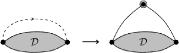
Figure 1. Injection from networks to vertex-rooted 2-connected SP graphs by adding one vertex and two edges.

We thus have $y^{3}\mathcal{D}(y)\preceq\mathcal{B}^{\prime}(y)\preceq u\mathcal{D}(y)$, which ensures that $\mathcal{B}^{\prime}(y)$ has the radius of convergence $\eta_{\mathcal{D}}$ and that $g(y)=\mathcal{B}^{\prime}(y)$ satisfies $g^{\prime}(y)\to\infty$ as $y\to\eta_{\mathcal{D}}^{-}$, since $\mathcal{D}(y)$ has a square-root expansion and hence $\mathcal{D}^{\prime}(y)\to\infty$ as $y\to\eta_{\mathcal{D}}^{-}$). This concludes that the class of labelled SP graphs is subcritical.

Now we turn to the unlabelled case, which is technically more involved. For each class $\mathcal{N}\in\{\mathcal{D},\mathcal{S},\mathcal{P}\}$ of networks, the automorphisms have to fix each of the two poles $+$ and $-$, and the cycle index sum $Z_{\mathcal{N}}(s_{1},s_{2},s_{3},\ldots)$ is defined as a sum of monomials over all automorphisms, as in Section 2.1. We define $N=N(y,z):=Z_{\mathcal{N}}(y,f(z^{2}),f(z^{3}),\ldots)$. For networks, the automorphisms have to fix each of the two poles $+$ and $-$. However, it is also useful to consider networks up to exchanging the poles and their corresponding series $\overline{Z}_{\mathcal{N}}(s_{1},s_{2},s_{3},\ldots)$ defined similarly as the cycle index sum, but summing over the automorphisms exchanging $+$ and $-$ (instead of those fixing $+$ and $-$ as in the series $Z_{\mathcal{N}}$). Define the bivariate series $\overline{N}=\overline{N}(y,z):=\overline{Z}_{\mathcal{N}}(y,f(z^{2}),f(z^{3}),\ldots)$ for each class $\mathcal{N}\in\{\mathcal{D},\mathcal{S},\mathcal{P}\}$ of networks. For a bivariate series $f(y,z)$ and $k\geq 1$ define $f^{(k)}(y,z):=f(y^{k},z^{k})$. The decomposition for pole-fixing networks and pole-exchanging networks give rise to explicit systems for the cycle index sums. Under the specialization $(s_{1}=y,s_{2}=f(z^{2}),s_{3}=f(z^{3}),\ldots)$, these yield the two systems (where the argument $(y,z)$ of the series is omitted):

$${\mathrm{(PF)}}\displaystyle\left\{\begin{array}[]{rcl}\vspace{0.05cm}\par\vspace{0.05cm}\par\vspace{0.05cm}\par\displaystyle D&=&1+S+P,\\ \displaystyle S&=&y\cdot D\cdot(1+P),\\ \displaystyle P&=&2\exp\left(\displaystyle\sum\nolimits_{i\geq 1}\frac{1}{i}S^{(i)}\right)-S-2,\end{array}\right.$$

and for the pole-exchanging networks

$${\mathrm{(PE)}}\displaystyle\left\{\begin{array}[]{rcl}\vspace{0.05cm}\par\vspace{0.05cm}\par\vspace{0.05cm}\par\vspace{0.05cm}\par\vspace{0.05cm}\par\vspace{0.05cm}\par\displaystyle\overline{D}&=&1+\overline{S}+\overline{P},\\ \displaystyle\overline{S}&=&D^{(2)}\cdot(y+f(z^{2})(1+\overline{P})),\\ \displaystyle\overline{P}&=&2\exp\left(\displaystyle\sum\nolimits_{k\geq 1}\frac{S^{(2k)}}{2k}+\frac{\overline{S}^{(2k-1)}}{2k-1}\right)-\overline{S}-2.\end{array}\right.$$

The series $g(y,z):=Z_{\mathcal{B}^{\prime}}(y,f(z^{2}),f(z^{3}),\ldots)$ can be expressed in terms of the series in the above two systems (this is done in [19] using the dissymmetry theorem):

$$g(y,z) = \frac{1}{2}y^{2}(1+P)D+\frac{1}{2}f(z^{2})D^{(2)}\cdot\left(1+y+yP^{(2)}+\overline{P}\right)+$$

$$2y\exp\left(\sum\nolimits_{i\geq 1}\frac{1}{i}S^{(i)}\right)-2y-2yS-\frac{1}{2}yS^{2}-\frac{1}{2}yS^{(2)}-ySP.$$

As in Lemma 14 we let $f(z):=\widetilde{\mathcal{C}^{\bullet}}(z)$, $g(y,z):=Z_{\mathcal{B}^{\prime}}(y,f(z^{2}),f(z^{3}),\ldots)$, and let $\rho$ be the radius of convergence of $f(z)$ and $\tau=f(\rho)$. In addition, we let $\eta_{D}(z)$ and $\eta_{\overline{D}}(z)$ be the singularity functions of $y\mapsto D(y,z)$ and $y\mapsto\overline{D}(y,z)$.

Lemma 16.

Each of the series $D(s,z),S(s,z),P(s,z)$ admits a square-root expansion at $(\eta_{D}(\rho),\rho)$.

Proof.

As $Z_{\mathcal{B}^{\prime}}(f(z),f(z^{2}),\ldots)$ counts derived connected SP graphs with a unique block incident to the pointed vertex and $f(z)$ counts all rooted SP graphs, we have $g(f(\rho),\rho)=Z_{\mathcal{B}^{\prime}}(f(\rho),f(\rho^{2}),f(\rho^{3}),\ldots)\leq f(\rho)$. In addition $f(\rho)<\infty$ since $f(z)$ is a solution of nonlinear functional equations. Hence $g(f(\rho),\rho)<\infty$. As $\mathcal{Z}^{3}\cdot\mathcal{D}\subseteq\mathcal{B}^{\prime}$ (see Figure 1) we have

$$u^{3}\ \!D(y,z)\preceq g(y,z).$$

Hence, by domination, $D(f(\rho),\rho)<\infty$ and therefore the singularity of $y\mapsto D(y,\rho)$ is larger than $f(\rho)$, which implies in particular that $z=\rho$ is an admissible valuation. The equation-system (PF) $\mathbf{F}(\mathbf{y};z)$ for $\mathbf{y}=(D,S,P,y)$ satisfies all conditions required in Theorem 2 (aperiodicity of $D$, strongly recursive system, analyticity of the functional system $\mathbf{F}(\mathbf{y};z)$ at the required point). Therefore the series $D$, $S$, and $P$ admit singular expansions at $(\eta_{D}(\rho),\rho)$. ∎

Lemma 17.

If $\eta_{D}(\rho)<\eta_{\overline{D}}(\rho)$ then the series $\overline{D}(s,z),\overline{S}(s,z),\overline{P}(s,z)$ are analytic at $(\eta_{D}(\rho),\rho)$, if not , then these series admit a square-root expansion at $(\eta_{\overline{D}}(\rho),\rho)$.

Proof.

Note that Figure 1 yields an injection from the pole-exchanging automorphisms of $\mathcal{D}$ to the automorphisms of $\mathcal{B}^{\prime}$. As a consequence, $s_{2}\overline{Z}_{\mathcal{D}}\preceq Z_{\mathcal{B}^{\prime}}$ so that

$$z^{2}\overline{D}(y,y)\preceq g(y,z).$$

Hence, $Z_{\mathcal{B}^{\prime}}(f(\rho),f(\rho^{2}),f(\rho^{3}),\ldots)=\tau<\infty$ implies that $\overline{D}(f(\rho),\rho)<\infty$. Therefore $\eta_{\overline{D}}(\rho)\geq f(\rho)$ so that $z=\rho$ is an admissible valuation for $\overline{D}(y,z)$. Note that the functional system (PE) $\mathbf{G}(\mathbf{y};z)$ with $\mathbf{y}=(\overline{D},\overline{S},\overline{P},y)$ is clearly analytic at a given point $(\overline{D},\overline{S},\overline{P},y;z)$ (where $\overline{D}$, $\overline{S}$, $\overline{P}$ are seen as independent variables) if and only if $D$ is analytic at $(y^{2},z^{2})$ and $f$ is analytic at $z^{2}$. Since $\rho<1$ and $\eta_{\mathcal{D}}(z)$ is decreasing in $z$, $\mathbf{G}$ is analytic at any point such that $|y|\leq\eta_{D}(\rho)$ and $|z|\leq\rho$. Therefore, the only cause of singularity for $\overline{D}$ in this domain is a branch point (i.e., a solution of the singularity system). From Theorem 2, we conclude that in such a situation, $\overline{D}$, $\overline{S}$, and $\overline{P}$ have a square-root expansion at $(\eta_{\overline{D}}(\rho),\rho)$. ∎

Lemma 18.

The class of unlabelled series-parallel graphs is subcritical.

Proof.

We need to check that all four criteria in Lemma 14 are satisfied. Easy upper and lower bounds imply that $\rho\in(0,1)$, so the criterion (1) is satisfied. Let $\eta(z)$ the singularity function of $y\mapsto g(y,z)$. Expression for $g(y,z)$ in terms of the series of networks (pole-fixing and pole-exchanging), ensures that $\eta(z)=\mathrm{min}\{\eta_{D}(z),\eta_{\overline{D}}(z)\}$ for $z>0$. Hence $\eta(z)$, as the minimum of two continuous functions, is also continuous at $\rho$, so the criterion (3) is verified. If $\eta(\rho)=\eta_{D}(\rho)$ (the most likely case), then $\lim_{y\to\eta(\rho)^{-}}g_{y}(y,\rho)=\infty$ because $y^{3}D(y,z)\preceq g(y,z)$ and because the square-root expansion of $D(y,z)$ at $(\eta(\rho),\rho)$ yields $\lim D_{y}(y,\rho)=\infty$ as $y\to\eta(\rho)$. If $\eta(\rho)=\eta_{\overline{D}}(\rho)$, then applying Lemma 17 $\overline{D}(y,z)$ has a square-root expansion at $(\eta(\rho),\rho)$. Again we have $\lim g_{y}(y,\rho)=\infty$ as $y\to\eta(\rho)$ because $z^{2}\overline{D}(y,z)\preceq g(y,z)$ and because the square-root expansion of $\overline{D}(y,z)$ at $(\eta(\rho),\rho)$ yields $\lim\overline{D}_{y}(y,\rho)=\infty$ as $y\to\eta(\rho)$. Thus the criterion (2) is verified.

It remains to check the criterion (4). From the work in [8, 19] one can extract an expression for $K(y,z):=Z_{\mathcal{B}}(y,f(z^{2}),f(z^{3}),\ldots)$ (longer than the one of $g(y,z)$, but of the same aspect) in terms of the series $\{D,S,P,\overline{D},\overline{S},\overline{P}\}$. This ensures that the singularity function $\eta_{H}(z)$ of $y\mapsto H(y,z)$ satisfies $\eta_{H}(z)=\mathrm{min}\{\eta_{D}(z),\eta_{\overline{D}}(z)\}=\eta(z)$. Since $\eta_{H}(\rho)\geq f(\rho)$ and since $\eta_{H}$ is continuous at $\rho$, we have $\eta_{H}(z)>0$ for $z$ around $\rho$. Hence $H(0,z)$ is analytic at $\rho$. In addition one can show that $Z_{\mathcal{C}}(0,z^{2},z^{3},\ldots)=Z_{\mathcal{B}}(0,f(z^{2}),f(z^{3}),\ldots)$, see [19] (a combinatorial interpretation is that if there is no fixed vertex in an automorphism $\sigma$ of a connected graph, then there is a unique 2-connected block $B$ fixed by $\sigma$, and the automorphism induced on $B$ has no fixed vertex as well). Hence $q(z)=Q(0,z)=H(0,z)$, which ensures that $q(z)$ is analytic at $\rho$. ∎

6.4. Graphs defined by their $3$-connected components.

The same arguments used in the enumeration of the unlabelled SP-graphs can be adapted to get similar results for families of graphs which are defined by a finite set of $3$-connected components (see [21] for a proper definition of these families). In these families, the strategy used is the same as in SP-graphs: we study the enumeration of networks in order to get the asymptotic counting of the graphs with a lower level of connectivity. The main difference is that there is an additional line in the equation-system for networks, which involves the Walsh polynomial (roughly speaking, the cycle index sum associated to the finite family of $3$-connected components; see [18, 19] for a detailed definition). The Walsh polynomial has two kinds of variables: $e_{1},\ldots,e_{r}$ and $\overline{e_{1}},\ldots,\overline{e_{k}}$. In the equation-system for networks, these variables are to be substituted by $D^{(1)},\ldots,D^{(r)}$ and by $\overline{D}^{(1)},\ldots,\overline{D}^{(k)}$, respectively (in SP-graphs this polynomial vanishes, because SP-graphs do not have $3$-connected components). Since the Walsh polynomial is an entire function in all its variables and has positive coefficients, the system remains positive and the argument of Lemmas 17, 18 can be adapted to this general setting in order to assure a square-root singularity for the counting series associated to networks, and the rest of the results can be easily adapted to this general framework.

7. Limit laws

In this section we study the limit distribution of a graph parameter defined on a uniformly distributed random graph on $n$ vertices. More concretely, let $X_{n}$ be the associated random variable. We show that all the parameters under study invariably converges in distribution to a normal limit distribution in the form

$$\frac{X_{n}-\mathbb{E}\,X_{n}}{\sqrt{\mathbb{V}{\mathrm{ar}}\,X_{n}}}\to N(0,1),$$

where $\mathbb{E}\,X_{n}=\mu n+O(1)\quad\mbox{and}\quad\mathbb{V}{\mathrm{ar}}\,X_{n}=\sigma^{2}n+O(1)$ for computable constants $\mu,\sigma^{2}>0$. The main results used in this section are Theorem $2.23$ of [11] (adapted in this paper as Theorem 3). In order to decide whether $\sigma^{2}>0$ we can either calculate it directly or use Lemma 4. For example, we can check the conditions of Lemma 4 with the help of small values of $n,m,k$. This applies for all kinds of graphs and parameters we consider here. However, in any case (if $\sigma^{2}=0$ or $\sigma^{2}>0$) these parameters are concentrated around its expected value.

The parameters discussed in this section are the number of edges, the number of blocks and the number of cut-vertices. All these parameters can be encoded in the generating function framework of the form

$$\mathcal{G}(z,v)=\exp(\mathcal{C}(z,v)),\,\,\mathcal{C}^{\bullet}(z,v)=F(\mathcal{C}^{\bullet}(z,v);z,v)$$

for the labelled case, and

$$\widetilde{\mathcal{G}}(z,v)=\exp\left(\sum\nolimits_{k\geq 1}\widetilde{\mathcal{C}}(z^{k},v^{k})/k\right),\,\,\widetilde{\mathcal{C}^{\bullet}}(z,v)=F(\widetilde{\mathcal{C}^{\bullet}}(z,v);z,v)$$

for the unlabelled case. In both cases, $z$ marks vertices and $v$ marks the parameter under study. The singularity curve $z=\rho(v)$ for the GF associated to general graphs is the same as the one for connected graphs, because both functions $\exp$ and $\overline{\exp}$ are analytic functions. As a consequence, the same limit law holds for both general and connected graphs (hence we can restrict our study to connected graphs). In order to study these limit laws we analyse the characteristic system

(15) $$y=F(y;z,v),\,\,\,1=\frac{\partial F}{\partial y}(y;z,v).$$

Observe that we recover the univariate system $y=F(y;z),\,\,\,1=\partial F/\partial y(y;z)$ by evaluating (15) at $v=1$. For the classes under study we have shown that this univariate system of equations is analytically well-founded (in the sense of Definition 1), hence by Theorem 2, $y(z,1)$ is the unique solution and has a square-root expansion around its smallest real singularity. This expansion can be extended to a real neighbourhood of $v=1$ with expression $y(z,v)$.

In this section we obtain the exact parameters for the labelled case. Unfortunately in the unlabelled framework there are no explicit formulas for the expectation and the variance, hence we content ourselves with the normal condition derived from Theorem 3 combined with Lemma 4. Finally, local limit laws are also discussed for these parameters.

7.1. The labelled case

The labelled case have been partially treated in [21], where the authors developed a case-by-case analysis. In this section we rediscover these results using a different and more general argument. Recall that $\tau=\mathcal{C}^{\bullet}(\rho)$ is the unique solution of the equation $y\mathcal{B}^{\prime\prime}(y)=1$ on the region where $\mathcal{B}(y)$ is analytic, and $\rho$ is the radius of convergence of $\mathcal{C}(z)$.

We use a secondary variable $v$ to mark edges. For a graph class $\mathcal{G}$ we write $\mathcal{G}=\cup_{n,m}\mathcal{G}_{n,m}$, where $n$ denotes the number of vertices and $m$ denotes the number of edges. We define the bivariate generating function as

$$\mathcal{G}(z,v)=\sum_{n,m}\frac{1}{n!}|\mathcal{G}_{n,m}|z^{n}v^{m}.$$

The series is exponential according to the (labelled) vertices and ordinary according to the (unlabelled) edges. A similar definition can be stated for both connected and $2$-connected graphs in $\mathcal{G}$ ($\mathcal{C}(z,v)$ and $\mathcal{B}(z,v)$ respectively). For a block-stable graph class $\mathcal{G}$, the block-decomposition translates to

$$\mathcal{C}^{\bullet}(z,v)=z\ \!\exp(\mathcal{B}^{\prime}(\mathcal{C}^{\bullet}(z,v),v)),$$

where $\mathcal{B}^{\prime}(z,v)$ denotes the derivative of $\mathcal{B}(z,v)$ with respect to the first variable. Observe that we need to deal with the bivariate GF associated to 2-connected graphs of the class. All subcritical classes under study are subclasses of planar graphs, hence the number of edges is linear. Consequently the subcritical condition is stable under a slight variation of $v$ around $v=1$. We denote by $\mathcal{B}_{v}^{\prime}(z,v)=\frac{\partial}{\partial v}\mathcal{B}^{\prime}(z,v)$, the derivative of $\mathcal{B}^{\prime}(z,v)$ with respect to the second variable.

The next parameter considered is the number of blocks, which is coded by the following equation

$$\mathcal{C}^{\bullet}(z,u)=z\ \!\exp\left(u\mathcal{B}^{\prime}(\mathcal{C}^{\bullet}(z,u))\right),$$

where the secondary variable $u$ marks the number of blocks. Finally, for the number of separating vertices, also called cut-vertices, we consider the bivariate GF

$$\mathcal{C}^{\bullet}(z,w)=z\ \!w\ \!(\exp\left(\mathcal{B}^{\prime}\left(\mathcal{C}^{\bullet}(z,w)\right)\right)-1)+z.$$

Observe however that $w$ does not mark exactly the number of separating vertices, as the root-vertex is always considered as a cut-vertex. However, the limit law for the number of cut-vertices does not depend on the behaviour of a single vertex.

All the results are contained in Table 2. Despite the methodology used here (direct application of Theorem 3) is different from the one of [21], the parameters we obtain are the same.

Parameter $$F(y;z,v)$$

Edges

Blocks

Cut-vertices

Table 2. Parameters with the corresponding value of $\mu$ and $\sigma^{2}$.

7.2. The unlabelled case

The same arguments used in the labelled framework work for GFs in the unlabelled framework, and Theorem 3 assures asymptotic normal limit distributions (with a non-vanishing variance) for these parameters. However, in this setting, expressions for the derivatives of $F$ are much involved, and consequently expressions for $\mu$ and $\sigma$ are complex. We cannot obtain closed expressions (as the ones in Table 2) for both the expectation and the variance of the resulting random variables.

Using the techniques introduced in Section 9 one can find numerical approximations for the derivatives of the function $F(y;z,v)$. Such computations are conducted in [4] for the number of edges in random unlabelled outerplanar graphs.

7.3. Local limit laws

In addition to the central limit laws described above, (much stronger) local limit laws hold for the parameters under study, either in the labelled or the unlabelled framework. The main results used here are (6) and the asymptotic estimates for both $[z^{n}]\mathcal{C}^{\bullet}(z)$ and $[z^{n}]\widetilde{\mathcal{C}^{\bullet}}(z)$. For conciseness, we state the result for connected graphs, but a similar result is also valid for general graphs.

Theorem 19.

Let $\mathcal{G}$ be a subcritical graph class with the property that $[z^{n}]\mathcal{C}(z)>0$ for $n\geq n_{0}$. Let $X_{n}$ be a random variable for a graph parameter studied above (the number of edges, blocks, or cut-vertices) defined on a random uniformly distributed connected graph of $\mathcal{G}$ on $n$ vertices and assume that $\sigma^{2}>0$. Let $m=\mu n+O(n^{1/2})$. Then

$$\mathbb{P}\left(X_{n}=m\right)=\frac{1}{\sqrt{2\pi n}\sigma}e^{-(m-\mu n)^{2}/(2\sigma^{2}n)}\left(1+O(n^{-1/2})\right).$$

Proof.

In all cases under study assumptions stated in the remark following the proof of Lemma 4 holds. The result is obtained by dividing the estimate in (6) by either $[z^{n}]\mathcal{C}^{\bullet}(z)$ or $[z^{n}]\widetilde{\mathcal{C}^{\bullet}}(z)$. ∎

8. Degree distribution

In this section we discuss the degree distribution of graphs of a subcritical graph family. We denote by $X_{n}^{k}$ and $\widetilde{X}_{n}^{k}$ the random variables which count the number of vertices of degree $k$ in a randomly chosen member of size $n$ of the family $\mathcal{G}$ and $\widetilde{\mathcal{G}}$, respectively. We further denote by $d_{k}$ and $\widetilde{d}_{k}$ the probability that the root vertex of a randomly chosen member of $\mathcal{G}^{\prime}$ or $\widetilde{\mathcal{G}}^{\prime}$ is $k$. The main tool to obtain asymptotic results is the analogue on systems of equations of Theorem 3.

8.1. The labelled case

Consider the series

$$B_{j}^{\prime}(z,\mathbf{v})=\sum_{n,n_{1},\ldots,n_{k},n_{\infty}}b_{j;n;n_{1},\ldots,n_{k},n_{\infty}}^{\prime}v_{1}^{n_{1}}\cdots v_{k}^{n_{k}}v_{\infty}^{n_{\infty}}\frac{z^{n}}{n!},$$

where we use the notation $\mathbf{v}=(v_{1},\ldots,v_{k},v_{\infty})$ and $b_{j;n;n_{1},\ldots,n_{k},n_{\infty}}^{\prime}$ is the number of derived 2-connected graphs with $1+n=1+n_{1}+\cdots+n_{k}+n_{\infty}$ vertices such that one vertex of degree $j$ is marked and the remaining $n$ vertices are labelled by $1,2,\ldots,n$ and $n_{\ell}$ vertices have degree $\ell$, $1\leq\ell\leq k$, and $n_{\infty}$ vertices have degree greater than $k$. By definition we have

$$B^{\prime}(z)=\sum_{2\leq j\leq\infty}B_{j}^{\prime}(z,\mathbf{1}).$$

Hence the radius of convergence of the functions $B_{j}^{\prime}(z,\mathbf{1})$ is greater or equal than the radius of convergence of $B^{\prime}(z)$.

We introduce an analogous series

$$C_{j}^{\prime}(z,\mathbf{v})=\sum_{n,n_{1},\ldots,n_{k},n_{\infty}}c_{j;n;n_{1},\ldots,n_{k},n_{\infty}}^{\prime}v_{1}^{n_{1}}\cdots v_{k}^{n_{k}}v_{\infty}^{n_{\infty}}\frac{z^{n}}{n!},$$

for derived connected graphs. We further set

$$B^{\prime}(z,w)=\sum_{j}B_{j}^{\prime}(z,\mathbf{1})w^{j}=\sum_{n,j}b^{\prime}_{n,j}z^{n}w^{j},$$

and $b^{\prime}_{n,j}$ is the number of derived $2$-connected graphs with $n+1$ vertices such that one vertex of degree $j$ is marked and the remaining $n$ vertices are labelled by $1,2,\ldots,n$. Analogously, we define the function $C^{\prime}(z,w)=\sum_{j}C^{\prime}_{j}(z,\mathbf{1})w^{j}$. According to the block decomposition of connected graphs

$$C^{\prime}(z,w)=\exp(B^{\prime}(zC^{\prime}(z),w)).$$

In the following, we set $B_{j}^{\prime}(z):=B_{j}^{\prime}(z,\mathbf{1})$. We will also use the series $B(z,\mathbf{v})$, which is the refined version of the generating function $B(z)$ of unrooted blocks taking into account all vertex degrees.

Theorem 20.

Let $\mathcal{G}$ be a family of random subcritical graphs (such that $[z^{n}]\,\mathcal{C}(z)>0$ for $n\geq n_{0}$) and $\mathcal{G}^{\prime}$ be its derived family. Then for $k$ fixed,

1. the limiting probability $d_{k}$ that the pointed vertex of a member of $\mathcal{G}^{\prime}$ has degree $k$ exists and is given by

   $$d_{k}=\rho\left(\sum_{i=1}^{k}B_{i}^{\prime\prime}\left(\rho C^{\prime}(\rho)\right)C_{k-i}^{\prime}(\rho)\right).$$

2. the random variable $X_{n}^{k}$ that counts the number of vertices of degree $k$ in a randomly chosen member of $\mathcal{G}$ satisfies a central limit theorem with mean $\mathbb{E}\,X_{n}^{k}=d_{k}n+O(1)$ and variance $\mathbb{V}{\mathrm{ar}}\,X_{n}^{k}=\sigma_{k}^{2}n+O(1)$, where $\sigma_{k}$ is a constant depending on $k$.

Proof of Theorem 20 (1).

We use the following lemma, which makes it easy to compute $d_{k}$. The proof is the same as the one for [11, Theorem 9.17].

Lemma 21.

The generating function $p(w)=\sum d_{k}w^{k}$ satisfies

$$p(w)=\rho e^{B^{\prime}(z,w)}\frac{\partial}{\partial z}B^{\prime}(z,w)\bigg{|}_{z=\rho C^{\prime}(\rho)},$$

and $p(1)=1$, thus the $d_{k}$’s define indeed a probability distribution.

Therefore, we have

$$d_{k} =[w^{k}]p(w)=[w^{k}]\rho e^{B^{\prime}(z,w)}\frac{\partial}{\partial z}B^{\prime}(z,w)\bigg{|}_{z=\rho C^{\prime}(\rho)}$$

$$=\rho\left(\sum_{i=0}^{k}[w^{k-i}]e^{B^{\prime}(z,w)}[w^{i}]\frac{\partial}{\partial z}B^{\prime}(z,w)\right)\bigg{|}_{z=\rho C^{\prime}(\rho)}$$

$$=\left(\sum_{i=1}^{k}\frac{\partial}{\partial z}B^{\prime}_{i}(z)[w^{k-i}]\left(1+\sum_{k}B_{k}^{\prime}(z)w^{k}+\frac{(\sum_{k}B_{k}^{\prime}(z)w^{k})^{2}}{2}+\cdots\right)\right)\bigg{|}_{z=\rho C^{\prime}(\rho)}$$

$$=\left(\sum_{i=1}^{k}\frac{\partial}{\partial z}B^{\prime}_{i}(z)\left(\sum_{m=1}^{k-i}\sum_{l_{1}+\cdots l_{m}=k-i}B_{l_{1}}(z)\cdots B_{l_{m}}(z)\right)\right)\bigg{|}_{z=\rho C^{\prime}(\rho)}.$$

From there the result follows, as the second term is exactly the representation of a connected graph of root degree $k-i$ according to the block decomposition, evaluated at $z=\rho$. ∎

Proof of Theorem 20 (2).

First we derive a system of functional equations which is satisfied by $C_{j}^{\prime}=C_{j}^{\prime}(z,\mathbf{v})$, and is refinement of

$$C^{\bullet}(z)=z\exp(B^{\prime}(C^{\bullet}(z))).$$

Lemma 22.

Let $W_{j}=W_{j}(z,\mathbf{v};C_{1}^{\prime},\ldots,C_{k}^{\prime},C_{\infty}^{\prime})$, $j\in\{1,2,\ldots,k,$ $\infty\}$ defined by

$$W_{j} =\sum_{i=0}^{k-j}v_{i+j}C_{i}^{\prime}(z,\mathbf{v})+v_{\infty}\left(\sum_{i=k-j+1}^{k}C_{i}^{\prime}(z,\mathbf{v})+C_{\infty}^{\prime}(z,\mathbf{v})\right),\qquad 1\leq j\leq k,$$

$$W_{\infty} =v_{\infty}\left(\sum_{i=0}^{k}C_{i}^{\prime}(z,\mathbf{v})+C_{\infty}^{\prime}(z,\mathbf{v})\right).$$

Set $\mathbf{W}=(W_{1},\ldots,W_{k},W_{\infty})$. Then the series $C_{1}^{\prime},\ldots,C_{k}^{\prime},C_{\infty}^{\prime}$ satisfy the system of equations

$$C_{j}^{\prime}(z,\mathbf{v}) =\sum_{\ell_{1}+\cdots j\ell_{j}=j}\ \prod_{r=1}^{j}\frac{B_{r}^{\prime}(z,\mathbf{W})^{\ell_{r}}}{\ell_{r}!},\qquad 1\leq j\leq k,$$

$$C_{\infty}^{\prime}(z,\mathbf{v}) =\exp\Biggl{(}\sum_{j=1}^{k}B_{j}^{\prime}(z,\mathbf{W})+B_{\infty}^{\prime}(z,\mathbf{W})\Biggr{)}-1-\sum_{1\leq\ell_{1}+\cdots k\ell_{k}\leq k}\ \prod_{r=1}^{k}\frac{B_{r}^{\prime}(z,\mathbf{W})^{\ell_{r}}}{\ell_{r}!}.$$

Proof.

As already indicated, the proof is a refined version of the functional equation fulfilled by $C^{\bullet}(z)$, which reflects the decomposition of a derived connected graph into a finite set of derived $2$-connected graphs, where every vertex (different from the root) is substituted by a derived connected graph. The functions $W_{j}$ serve the purpose of marking (recursively) the degree of the vertices in the 2-connected blocks which are substituted by other graphs. In the definition of $W_{j}$, the summation means that we are substituting a vertex of degree $i$, but since originally the vertex had degree $j$, we are creating a new vertex of degree $i+j$, which is marked accordingly by $v_{i+j}$. The analogous holds for $W_{\infty}$. ∎

To prove Theorem 20 (2) we observe

$$C^{\prime}(z)=\sum_{0\leq j\leq\infty}C_{j}^{\prime}(z,\mathbf{1}).$$

Furthermore, since the above system of equations is strongly connected, all functions $C_{j}^{\prime}(z,\mathbf{1})$ have the same radius of convergence as $C^{\prime}(z)$, as mentioned in Section 3.2. By assumption this radius of convergence is smaller than the radius of convergence of $B^{\prime}(z)$. Hence, by stability if $\mathbf{v}$ is sufficiently close to $\mathbf{1}$ then the the singularities of $B_{j}^{\prime}$ and $C_{j}^{\prime}$ do not interfere, in particular we can apply Theorem 2 and obtain that all functions $C_{j}^{\prime}$ have a square-root singularity. Finally, let

$$C^{(k)}(z,v)=\sum_{n,m}c_{k;n,m}v^{m}\frac{z^{n}}{n!}$$

be the generating function for the numbers $c_{k;n,m}$ of unrooted connected outerplanar graphs of size $n$ with $m$ nodes of degree $k$. Then $C^{(k)}(z,v)$ satisfies

$$\frac{\partial C^{(k)}(z,v)}{\partial z}=\sum_{j=1}^{k-1}C_{j}^{\prime}(z,1,\ldots,1,v,1)+vC^{\prime}_{k}(z,1,\ldots,1,v,1)+C^{\prime}_{\infty}(z,1,\ldots,1,v,1),$$

and thus $C^{(k)}(z,v)$ has a singular expansion of order $\frac{3}{2}$ around ${v}={1}$. Furthermore, the central limit theorem for the number of vertices of given degrees with mean $\mu_{k}n$ and variance $\sigma^{2}_{k}n$ follows by the analogue of Theorem 3 for systems of equations. It immediately follows that $d_{k}=\mu_{k}$ as there are exactly $n$ possible ways to root an unrooted object of size $n$ at one of the vertices and thus the probability that a random vertex has degree $k$ is exactly the same as the probability that the root vertex has degree $k$. Despite that, we could also use formula (7) to compute $\mu_{k}$, we would obtain the same value as for $d_{k}$ here. ∎

8.2. The unlabelled case

We introduce cycle index sums

$$Z_{\widetilde{\mathcal{B}}^{\prime}_{j}}(s_{1},s_{2},\ldots;v_{1,1},v_{1,2},\ldots;\ldots;v_{k,1},v_{k,2},\ldots;v_{\infty,1},v_{\infty,2},\ldots)$$

for the class of pointed blocks, where the pointed vertex has degree $j$ and is not counted, and where the variables $v_{i,j}$ count the cycles of length $j$ of vertices of degree $i$, and $v_{\infty,j}$ counts those vertices of degree greater than $k$. As in Section 8.1 let $\mathbf{v}=(v_{1},\ldots,v_{k},v_{\infty})$. Denote the corresponding OGFs by $\widetilde{B}^{\prime}_{j}(z,\mathbf{v}),j\in\{1,\dots,k,\infty\}$ and let

$$\widetilde{B}^{\prime}(z,\mathbf{v}):=\sum_{j=2}^{k}v_{j}\widetilde{B}^{\prime}_{j}(z,\mathbf{v})+v_{\infty}\widetilde{B}^{\prime}_{\infty}(z,\mathbf{v}).$$

Note that

$$Z_{\widetilde{\mathcal{B}}^{\prime}}(s_{1},s_{2},\ldots;1,1,\ldots;\ldots;1,1,\ldots;1,1,\ldots)=Z_{\widetilde{\mathcal{B}}^{\prime}}(s_{1},s_{2},\ldots),$$

and thus the singularity $\rho_{1}(\mathbf{v})$ of $\widetilde{B}^{\prime}(z,\mathbf{v})$ is the same as that of $\widetilde{B}^{\prime}(z)$ at $\mathbf{v}=\mathbf{1}$, and $\rho_{1}(\mathbf{v})$ is the dominant singularity of the system $\mathbf{\widetilde{B}^{\prime}}(z,\mathbf{v})=(\widetilde{B}^{\prime}_{j}(z,\mathbf{v}))_{j\in\{1,\dots,k,\infty\}}$.

We now introduce the multivariate generating functions

$$\widetilde{C^{\prime}_{j}}(z,\mathbf{v}) =\sum_{n;n_{1},\ldots,n_{k},n_{\infty}}\widetilde{c}_{i;n;n_{1},\ldots,n_{k},n_{\infty}}v_{1}^{n_{1}}\cdots v_{k}^{n_{k}}v_{\infty}^{n_{\infty}}z^{n}$$

where the coefficient $\widetilde{c}_{i;n;n_{1},\ldots,n_{k},n_{\infty}}$ denotes the number of elements of size $n$ of $\mathcal{C}^{\prime}$, where the pointed vertex has degree $j$ and with $n_{i},i\in\{1,\dots,k\}$, vertices of degree $i$ and $n_{\infty}$ vertices of degree greater than $k$. We further set

$$\widetilde{B}^{\prime}(z,w)=\sum_{j}\widetilde{B}_{j}^{\prime}(z,\mathbf{1})w^{j}=\sum_{n,j}\widetilde{b}^{\prime}_{n,j}z^{n}w^{j}$$

and

$$\widetilde{C}^{\prime}(z,w)=\sum_{j}\widetilde{C}_{j}^{\prime}(z,\mathbf{1})w^{j}=\sum_{n,j}\widetilde{c}^{\prime}_{n,j}z^{n}w^{j}.$$

As we need cycle indices for the block decomposition, we set

$$Z_{\widetilde{\mathcal{B}}^{\prime}}(s_{1},s_{2},\ldots;w)=\sum_{j}Z_{\widetilde{\mathcal{B}}_{j}^{\prime}}(s_{1},s_{2},\ldots)w^{j}.$$

Note that the variable $w$, which counts the degree of the root, is not involved in any permutation cycle. Then,

$$\widetilde{C}^{\prime}(z,w)=\exp\left(\sum_{\ell\geq 1}\frac{1}{\ell}Z_{\widetilde{\mathcal{B}}^{\prime}}(z^{\ell}C^{\prime}(z^{\ell}),z^{2\ell}C^{\prime}(z^{2\ell}),\ldots;w^{\ell})\right).$$

Theorem 23.

Let $\widetilde{\mathcal{G}}$ be a family of random subcritical graphs (such that $[z^{n}]\,\mathcal{C}(z)>0$ for $n\geq n_{0}$) and $\widetilde{\mathcal{G}}^{\prime}$ be it’s derived family. Further, let $\widetilde{d}_{k}$ be the limiting probability that the root vertex of a member of $\widetilde{\mathcal{G}}^{\prime}$ has degree $k$ and let $\widetilde{X}_{n}^{k}$ be the random variable that counts the number of vertices of degree $k$ in a randomly chosen member of $\widetilde{\mathcal{G}}$. Then

1. $\widetilde{d}_{k}=\rho\left(\sum_{i=1}^{k}\frac{\partial}{\partial z}Z_{\widetilde{\mathcal{B}}_{i}^{\prime}}(z,\rho^{2}\widetilde{C}^{\prime}(\rho^{2}),\rho^{3}\widetilde{C}^{\prime}(\rho^{3}),\ldots)\big{|}_{z=\rho C^{\prime}(\rho)}C_{k-i}^{\prime}(\rho)\right).$

2. $\widetilde{X}_{n}^{k}$ satisfies a central limit theorem with mean $\mathbb{E}\widetilde{X}_{n}^{k}=\widetilde{\mu}_{k}n+O(1)$ and variance $\mathbb{V}{\mathrm{ar}}\ \widetilde{X}_{n}^{k}=\widetilde{\sigma}_{k}^{2}n+O(1)$.

Remark 24.

In the unlabelled case, we cannot expect that $\widetilde{\mu}_{k}$ equals $\widetilde{d}_{k}$, as vertex-rooting is only possible at fixed points of permutations, and thus in unlabelled graphs $n\widetilde{g_{n}}\neq\widetilde{g^{\prime}_{n}}$.

Proof of Theorem 23 (1).

The proof is based on the following lemma:

Lemma 25.

The generating function $\widetilde{p}(w)=\sum\widetilde{d}_{k}w^{k}$ is equal to

$$\rho\frac{\partial}{\partial u}\exp\left(Z_{\widetilde{\mathcal{B}}^{\prime}}(u,z^{2}C^{\prime}(z^{2}),\ldots;w)+\sum_{\ell\geq 2}\frac{1}{\ell}Z_{\widetilde{\mathcal{B}}^{\prime}}(z^{\ell}C^{\prime}(z^{\ell}),z^{2\ell}C^{\prime}(z^{2\ell}),\ldots;w^{\ell})\right),$$

and $\widetilde{p}(1)=1$. That is, it defines indeed a probability distribution.

Proof.

We use [11, Lemma 2.26] with

$$f(z,w) =zC^{\prime}(z),$$

$$H(z,w,u) =\exp\left(Z_{\widetilde{\mathcal{B}}^{\prime}}(u,z^{2}C^{\prime}(z^{2}),\ldots;w)+\sum_{\ell\geq 2}\frac{1}{\ell}Z_{\widetilde{\mathcal{B}}^{\prime}}(z^{\ell}C^{\prime}(z^{\ell}),\dots;w^{\ell})\right),$$

and the same line of reasoning as in [11, Theorem 9.17] proves the first part of the lemma. For $\widetilde{p}(1)=H_{u}(\rho,1,\rho C^{\prime}(\rho))$ we obtain

$$\rho C^{\prime}(\rho)\frac{\partial}{\partial u}Z_{\widetilde{\mathcal{B}}^{\prime}}(u,\rho^{2}C^{\prime}(\rho^{2}),\ldots)\bigg{|}_{u=\rho C^{\prime}(\rho)}=1$$

by the implicit function representation of $C^{\prime}(z)$. ∎

Now we can determine $\widetilde{d}_{k}=[w^{k}]\widetilde{p}(w)$, which is equal to

$$\rho\ [w^{k}]\left[\exp\left(\sum_{\ell\geq 1}\frac{1}{\ell}Z_{\widetilde{\mathcal{B}}^{\prime}}(\rho^{\ell}\widetilde{C}^{\prime}(\rho^{\ell}),\ldots;w^{\ell})\right)\left(\frac{\partial}{\partial u}Z_{\widetilde{\mathcal{B}}^{\prime}}(u,\rho^{2}\widetilde{C}^{\prime}(\rho^{2}),\ldots;w)\right)_{u=\rho C^{\prime}(\rho)}\right].$$

Recalling $Z_{\widetilde{\mathcal{B}}^{\prime}}=\sum_{l\geq 1}Z_{\widetilde{\mathcal{B}}_{\ell}^{\prime}}$, we obtain that the previous expression can be written

$$\rho\ \sum_{i=1}^{k}\frac{\partial}{\partial{u}}Z_{\widetilde{\mathcal{B}}_{i}^{\prime}}(u,\rho^{2}\widetilde{C}^{\prime}(\rho^{2}),\ldots)\big{|}_{u=\rho C^{\prime}(\rho)}\cdot[w^{k-i}]\exp\left(\sum_{\ell\geq 1}\frac{1}{\ell}Z_{\widetilde{\mathcal{B}}^{\prime}}(\rho^{\ell}\widetilde{C}^{\prime}(\rho^{\ell}),\ldots;w^{\ell})\right).$$

Observe that the second term translates into $\widetilde{C}^{\prime}_{k-i}(\rho)$, as the following equality holds:

$$\exp\left(\sum_{\ell\geq 1}\frac{1}{\ell}Z_{\widetilde{\mathcal{B}}^{\prime}}(\rho^{\ell}\widetilde{C}^{\prime}(\rho^{\ell}),\ldots;w^{\ell})\right)=\widetilde{C}^{\prime}(\rho,w)=\sum_{j}\widetilde{C}_{j}^{\prime}(\rho,\mathbf{1})w^{j}=\sum_{j}\widetilde{C}_{j}^{\prime}(\rho)w^{j}.$$

∎

Proof of Theorem 23 (2).

As in the labelled case, we observe that the functions $\widetilde{C^{\prime}_{j}}(z,\mathbf{v})$ satisfy a system of equations, using a refinement of the block decomposition. In the following we will denote by $\sum_{i=r}^{k,\infty}F_{i}=\sum_{i=r}^{k}F_{i}+F_{\infty}$.

Lemma 26.

For each $j=1,2,\ldots,k,\infty$, let $W_{j}$ be defined by

$$W_{j}(z,\mathbf{v})=\sum_{i=0}^{k-\ell}v_{j+i}\widetilde{C}^{\prime}_{j}(z,\mathbf{v})+v_{\infty}\left(\sum_{i=k-j+1}^{k,\infty}\widetilde{C}^{\prime}_{i}(z,\mathbf{v})\right),$$

$$W_{\infty}(z,\mathbf{v})=v_{\infty}\left(\sum_{i=0}^{k,\infty}\widetilde{C}^{\prime}_{i}(z,\mathbf{v})\right).$$

Set $W_{j,i}=W_{j}(z^{i},v_{1}^{i},\ldots,v_{k}^{i},v_{\infty}^{i})$ and

$$\mathbf{W}^{(l)}=(W_{1,l},W_{1,2l},\ldots;\ldots;W_{k,l},W_{k,2l},\ldots;W_{\infty,l},W_{\infty,2l},\ldots).$$

We denote by $S_{n}(s_{1},s_{2},\ldots)$ the cycle index of the symmetric group on $n$ elements. Furthermore $S_{n}[Z_{\mathcal{B}}]$ denotes the substitution $s_{l}\leftarrow Z_{\mathcal{B}}(s_{l},s_{2l},\ldots;\mathbf{W}^{(l)}),l\geq 1$ in $S_{n}(s_{1},s_{2},\ldots)$.

Then the series $\widetilde{C^{\prime}_{1}},\ldots,\widetilde{C^{\prime}_{k}},\,\widetilde{C^{\prime}_{\infty}}$ satisfy the system of equations

$$\widetilde{C}^{\prime}_{j}(z,\mathbf{v}) =\sum_{l_{1}+2l_{2}+\cdots+jl_{j}=j}\ \prod_{r=1}^{j}S_{l_{r}}\left[Z_{\mathcal{B}^{\prime}_{r}}\right]_{(s_{i}=z^{i})},\quad 1\leq j\leq k$$

$$\widetilde{C}^{\prime}_{\infty}(z,\mathbf{v}) =\exp\left(\sum_{l\geq 1}\frac{1}{l}\left(\sum_{r=1}^{k}Z_{\mathcal{B}^{\prime}_{r}}\left(z^{l},z^{2l},\ldots;\mathbf{W}^{(l)}\right)+Z_{\mathcal{B}^{\prime}_{\infty}}\left(z^{l},z^{2l},\ldots;\mathbf{W}^{(l)}\right)\right)\right)-$$

$$\sum_{1\leq l_{1}+\cdots+kl_{k}\leq k}\ \prod_{r=1}^{j}S_{l_{r}}\left[Z_{\mathcal{B}^{\prime}_{r}}\right]_{(s_{i}=z^{i})}.$$

Remark 27.

The functions $W_{j,i}$ and thus the whole system can also be considered in terms of cycle index sums, using the cycle index sum

$$Z_{\widetilde{C}_{j}^{\prime}}(s_{1},s_{2},\ldots;v_{1,1},v_{1,2},\ldots;\ldots;v_{k,1},v_{k,2},\ldots;v_{\infty,1},v_{\infty,2},\ldots)$$

for rooted connected graphs. The root vertices in $W_{j,i}$ are fixed and thus have cycle length $1$. We will need this terminology in the proof of Lemma 29.

Proof.

As in the labelled case, we refine the recursive decomposition of graphs into it’s $2$-connected components. The functions $W_{j,i}$ plays the analogous role as in the labelled case, except that we need a second index for representing the cycles of different length appearing in the cycle indices. This directly leads to $\widetilde{C}^{\prime}_{j}(z,\mathbf{v})$ for $j=1,\ldots k$. For $\widetilde{C}^{\prime}_{\infty}(z,\mathbf{v})$ we obtain

$$\sum_{(l_{1},l_{2},\ldots,l_{k},l_{\infty})}\prod_{r=1}^{k}S_{l_{r}}\left[Z_{\mathcal{B}^{\prime}_{r}}\left(z,z^{2},\ldots;\mathbf{W}^{(1)}\right)\right]S_{l_{\infty}}\left[Z_{\mathcal{B}^{\prime}_{\infty}}\left(z,z^{2},\ldots;\mathbf{W}^{(1)}\right)\right]-$$

$$\ \sum_{l_{1}+\ldots+kl_{k}\leq k}\prod_{r=1}^{k}S_{l_{r}}\left[Z_{\mathcal{B}^{\prime}_{r}}\left(z,z^{2},\ldots;\mathbf{W}^{(1)}\right)\right],$$

where the first sum rewrites into the exponential term appearing in $\widetilde{C}^{\prime}_{\infty}(z,\mathbf{v})$. ∎

It is easily checked that the system is strongly connected as every $\widetilde{C}^{\prime}_{j}(z,\mathbf{v})$ depends on $\widetilde{C}^{\prime}_{\infty}(z,\mathbf{v})$ for $j\in\{1,\ldots,k\}$ and $\widetilde{C}^{\prime}_{\infty}(z,\mathbf{v})$ depends on all the values $j\in\{1,\ldots,k\}$. Obviously,

(16) $$\widetilde{C}^{\prime}(z)=\left[\sum_{j=1}^{k}v_{j}\widetilde{C}^{\prime}_{j}(z,\mathbf{v})+v_{\infty}\widetilde{C}^{\prime}_{\infty}(z,\mathbf{v})\right]_{\mathbf{v}=\mathbf{1}}.$$

Define

$$\widetilde{C}^{\prime}(z,\mathbf{v}):=\sum_{j=1}^{k}v_{j}\widetilde{C}^{\prime}_{j}(z,\mathbf{v})+v_{\infty}\widetilde{C}^{\prime}_{\infty}(z,\mathbf{v}).$$

Then the generating function of derived connected graphs of $\widetilde{\mathcal{G}}$, where the variable $v$ counts the nodes of degree $k$, is given by $\widetilde{C}^{\prime(k)}(z,v)=\widetilde{C}^{\prime}(z,\mathbf{v}_{k})$, where $\mathbf{v}_{k}=(1,1,\ldots,1,v,1)$.

Lemma 28.

$\widetilde{C}^{\prime(k)}(z,v)$ has a square-root singular expansion around its singularity $\rho_{2}(v)$ in a neighbourhood of $v=1$.

Proof.

By Equation (16) the singularity of the system $\mathbf{\widetilde{C}^{\prime}}(z,\mathbf{v})$ at $\mathbf{v}=\mathbf{1}$ is $\rho_{2}$, the same as that of $\widetilde{C}^{\prime}(z)$. As the system is strongly connected, every $\widetilde{C}^{\prime}_{j}(z,\mathbf{1})$ has radius of convergence $\rho_{2}$. Since $\widetilde{C}^{\prime(k)}(z,1)$ is a linear combination of these functions, it has the same singularity, which fulfills $\rho_{2}\widetilde{C}^{\prime}(\rho_{2})<\rho_{1}$ due to the subcriticality assumption. By the stability property of subcriticality it follows that $(\widetilde{C}^{\prime(k)}(z,v),\widetilde{B}^{\prime(k)}(z,v))$ is subcritical near $1$, and hence we obtain a square-root singular expansion. ∎

Consider the cycles index sums

$$Z_{\widetilde{\mathcal{C}}}(s_{1},s_{2},\ldots;v_{1,1},v_{1,2},\ldots;\ldots;v_{k,1},v_{k,2},\ldots;v_{\infty,1},v_{\infty,2},\ldots)$$

for (unpointed) connected graphs of $\widetilde{\mathcal{G}}$. By taking $s_{1}=s$, $s_{i}=z^{i}$ for $i\geq 2$, $v_{j,i}=1$ for $1\leq j<k,i\geq 1$ and $v_{k,i}=v^{i}$ for $i\geq 1$ we obtain its corresponding OGF $\widetilde{C}^{(k)}(z,v)=Z_{\widetilde{\mathcal{C}}}(z,z^{2},\ldots;1,1,\ldots;\ldots;v,v^{2},\ldots;1,1,\ldots)$, where the variable $v$ counts the nodes of degree $k$.

Lemma 29.

$\widetilde{C}^{(k)}(z,v)$ has a singular expansion of order $\frac{3}{2}$ around its singularity $\rho_{2}(v)$ in a neighbourhood of $v=1$.

Proof.

We have to express the system of equations in Lemma 26 in terms of cycle index sums and analyze the trivariate generating functions

$$\widetilde{C}^{(k)}(s,z,v)=Z_{\widetilde{\mathcal{C}}}(s,z^{2},z^{3},\ldots;1,1,\ldots;\ldots;v,v^{2},\ldots;1,1,\ldots).$$

Obviously, $\widetilde{C}^{(k)}(z,z,v)=\widetilde{C}^{(k)}(z,v)$. Analogously we define $\widetilde{C}^{\prime(k)}(s,z,v)$. We obtain

$$\widetilde{C}^{(k)}(s,z,v)=\widetilde{C}^{(k)}(0,z,v)+\int_{0}^{z}\widetilde{C}^{\prime(k)}(s,z,v)\mathrm{d}s,$$

by the same arguments as in Section 5. Due to stability, we obtain a square-root singular expansion for $\widetilde{C}^{\prime(k)}(s,z,v)$ as before, with a singular term of the form $(1-s/\bar{\rho}(z,v))^{1/2}$. Integration and subcriticality conditions lead to a singular expansion of the form

$$\widetilde{C}^{(k)}(s,z,v)=a(s,z,v)+b(s,z,v)\left(1-\frac{s}{\bar{\rho}(z,v)}\right)^{3/2}.$$

At $s=z$ we can represent the singular part as

$$\left(1-\frac{z}{\bar{\rho}(z,v)}\right)^{3/2}=\kappa(z,v)\left(1-\frac{z}{\tilde{\rho}_{2}(v)}\right)^{3/2},$$

with an analytic factor $\kappa(z,v)$ and some analytic function $\tilde{\rho}(v)$. Since the singular manifold of $\widetilde{C}^{\prime(k)}(s,z,v)$ is the same as that of $\widetilde{C}^{(k)}(z,v)$, that is $z=\bar{\rho}(z,v)$ if and only if $z=\rho_{2}(v)$, it follows that $\tilde{\rho}(v)=\rho_{2}(v)$. ∎

Now, with the singular expansion in $\rho(v)$ given, we can immediately deduce a central limit law by the analogue to Theorem 3 for systems of equations. ∎

To calculate $\widetilde{\mu}_{k}$ we can use Expression (7). The derivatives give

$$\mathbf{b^{T}}\mathbf{F}_{v}(\mathbf{C}(\rho,1);\rho,1) =\left(E\cdot\sum_{j=1}^{k,\infty}\sum_{i=1}^{k}(B^{\prime}_{j})_{v_{i}}(z,\mathbf{W})y_{k-i}\right)\bigg{|}_{(\mathbf{C}(\rho,1);\rho,1)},$$

$$\mathbf{b^{T}}\mathbf{F}_{z}(\mathbf{C}(\rho,1);\rho,1) =\left(E\cdot\sum_{j=1}^{k,\infty}(B^{\prime}_{j})_{z}(z,\mathbf{W})\right)\bigg{|}_{(\mathbf{C}(\rho,1);\rho,1)},$$

where $y_{k-i}$ denotes the $(k-i)$-th coordinate of $\mathbf{y}$ satisfying $\mathbf{y}=\mathbf{F}(\mathbf{y};z,\mathbf{v})$, $(B^{\prime}_{j})_{v_{i}}$ is the derivative of $B^{\prime}_{j}$ with respect to $v_{i}$ and $E$ is the exponential term appearing in $\widetilde{C}^{\prime}_{\infty}$. As the formula includes all partial derivatives of $(\widetilde{B}^{\prime}_{j})$, we see that the calculation of $\widetilde{\mu}_{k}$ will be very involved and it is (in general) not equal to $\widetilde{d}_{k}$.

9. Computing the growth rate

In this section we show how to compute the exponential growth of unlabelled $2$-connected, connected and general SP-graphs, respectively. The main tool is the decomposition grammar and the systems of functional equations developed in Section 6.3.

We will first review the growth constants for subcritical classes of graphs in Section 9.1. Next we will approximate the exponential growth for the number of unlabelled SP-graphs in two steps: the first step for $2$-connected unlabelled SP-graphs (Section 9.2) and the second step for unlabelled connected SP-graphs (Section 9.3). To this end, we start with a functional system of the form $\textbf{y}=\textbf{F}_{N}(\textbf{y};z)$, which is a truncated version (combined with iteration) of the original functional system $\textbf{F}(\textbf{y};z)$ determining y and provides an approximation of y. The solution of this system, together with the additional restriction given by a singular equation (given by the determinant of the Jacobian of the previous system) gives the desired growth constant.

The error introduced in the computations becomes smaller as soon as we take a better approximation for y (in other words, more terms on the Taylor series of its components). We refer the reader to [4] and [28], in which the authors study a similar iterative scheme.

9.1. Explicit growth constants

The computation of the growth constant for the classes under study is based on the subcritical condition. In labelled case, the singularity $\rho$ is given by the equation $\rho=\tau\exp\left(-\mathcal{B}^{\prime}(\tau)\right)$, where $\tau$ is the smallest solution of the equation $y\mathcal{B}^{\prime\prime}(y)=1$. In case of unlabelled case, the growth constants obtained earlier in the literature are based on explicit expressions for $Z_{\mathcal{B}^{\prime}}(s_{1},s_{2},\dots)$, e.g. the classes of cacti graphs and outerplanar graphs. Here we will show how to derive the growth constants of SP graphs, even when there is not an explicit expression for $Z_{\mathcal{B}^{\prime}}(s_{1},s_{2},\dots)$.

We have shown in Theorem 15 that the asymptotic number of cacti, outerplanar and SP graphs is of the form $c\ \!n^{-5/2}\ \!\rho^{-n}\ \!n!\ \!(1+o(1))$ in the labelled case and is of the form $c\ \!n^{-5/2}\ \!\rho^{-n}\ \!(1+o(1))$ in the unlabelled case. In both cases (either labelled or unlabelled) the subexponential term $n^{-5/2}$ suggests that all these classes have an arborescent structure. In Table 3 the exponential growth constant $\rho^{-1}$ for connected (and general) acyclic, cacti, outerplanar and SP-graphs are shown.

Family	Labelled	Unlabelled
Acyclic	$2.71828$	$2.95577$
Cacti	$4.18865$	$4.50144$
Outerplanar	$7.32708$	$7.50360$
Series-Parallel	$9.07359$	$9.38527$

Table 3. Exponential growth for distinct subcritical classes. All constants are referred to connected and general classes.

9.2. Parameters for 2-connected SP-graphs.

First we compute the growth constant using the equations for networks (and related classes). Later, the resulting singularity is transferred to the counting series of $2$-connected SP-graphs $Z_{\mathcal{B}}(z,z^{2},z^{3},\dots)$.

Denote by $Z_{\mathcal{S}}(s_{1},s_{2},\dots)$, $Z_{\mathcal{P}}(s_{1},s_{2},\dots)$ and $Z_{\mathcal{D}}(s_{1},s_{2},\dots)$ the cycle index sums associated to series, parallel and general networks. Let $S(z)=Z_{\mathcal{S}}(z,z^{2},\dots)$, $P(z)=Z_{\mathcal{P}}(z,z^{2},\dots)$, $D(z)=Z_{\mathcal{D}}(z,z^{2},\dots)$. As it is shown in Section 6, the system of equations which defines series, parallel and general networks is

(17) $$\left\{\begin{array}[]{rcl}D(z)&=&1+S(z)+P(z),\\ S(z)&=&zD(z)\left(1+P(z)\right),\\ P(z)&=&2\exp\left(\sum_{i\geq 1}\frac{1}{i}S^{(i)}(z)\right)-S(z)-2.\end{array}\right.$$

Let $U(z)=\exp\left(\sum_{i\geq 2}\frac{1}{i}S^{(i)}(z)\right)$. This function is analytic at the singularity of $S(z)$. We can isolate $S(z)$ from System (17) and obtain the implicit relation

$$S(z)=z\left(2\exp(S(z))U(z)-1\right)\left(2\exp(S(z))U(z)-1-S(z)\right).$$

Observe that $U(z)$ depends on $S(z)$. In order to get an approximation of the smallest singularity of $S(z)$, we start looking for an approximation of $S(z)$. This can be done in the following way: let $S_{0}(z)=0$ and $U_{0}(z)=1$. Let $N$ be a positive integer. For a function $f(z)$, analytic at the origin, define $\mathrm{\texttt{pol}}_{N}\left\{f(z)\right\}$ as the Taylor polynomial of degree $N$ of $f(z)$. Define $S_{k+1}(z)$ and $U_{k+1}(z)$ recursively in the following way:

$$\left\{\begin{array}[]{rcl}S_{k+1}(z)&=&\mathrm{\texttt{pol}}_{N}\left\{z\left(2\exp(S_{k}(z))U_{k}(z)-1\right)\left(2\exp(S_{k}(z))U_{k}(z)-1-S_{k}(z)\right)\right\},\\ U_{k+1}(z)&=&\mathrm{\texttt{pol}}_{N}\left\{\exp\left(\sum_{i=2}^{N}\frac{1}{i}S_{k+1}^{(i)}(z)\right)\right\}.\end{array}\right.$$

We stop when $S_{k-1}(z)=S_{k}(z)$ (equivalently, when $S_{k}(z)=\mathrm{\texttt{pol}}_{N}\{S(z)\}$). Denote then $u(z)=\exp\left(\sum_{i=2}^{N}\frac{1}{i}S_{k}^{(i)}(z)\right)$, and consider the solution $s(z)$ of the equation

$$s(z)=z\left(2\exp(s(z))u(z)-1\right)\left(2\exp(s(z))u(z)-1-s(z)\right).$$

Taking $u(z)$ instead of $U(z)$ introduces an error, which can be controlled in that the larger $N$ is, the smaller the error. Under these assumptions, $s(z)$ is defined by an equation of the form $s=H(s;z)$, with $H(y;z)=z(2\exp(y)u(z)-1)(2\exp(y)u(z)-1-y)$. Consequently, we find its smallest singularity by solving the characteristic system $y=H(y;z),\,1=H_{y}(y;z)$. In Table 4 the values obtained for several choices are shown. In particular, one can observe that the accuracy in the computation are improved by increasing the order of truncation.

$N$	Singular point ($\rho$)
$5$	$\textbf{0.124}21863192426192376$
$10$	$\textbf{0.124199}19715484630978$
$20$	$\textbf{0.12419909378}526277564$
$50$	0.12419990937841528588

Table 4. Values for $N$ and the corresponding value for $\rho$.

These computations give the truncated value of $z$, $\rho_{1}\approx 0.12420$. This constant is slightly smaller than the one which is obtained in the labelled case (whose value is approximately $0.12800$. See [5]). This singularity is the same for the parallel family and for general networks. Using the same ideas one finds that the smallest singularity for exchanging poles networks is strictly bigger than $\rho_{1}$. Consequently, applying the transfer theorems of singularity analysis we conclude that the number $\widetilde{b_{n}}$ of $2$-connected unlabelled series-parallel graphs on $n$ vertices is

$$\widetilde{b_{n}}=\widetilde{b}\ \!n^{-3/2}\ \!\gamma_{1}^{n}\ \!(1+o(1)),$$

where $\gamma_{1}=\rho_{1}^{-1}\approx 8.05159$ and $\widetilde{b}$ is a constant.

9.3. Parameters for connected SP-graphs.

In order to approximate the growth constant for connected SP-graphs, we need to refine the analysis over the cycle index sum for pointed 2-connected unlabelled SP-graphs, which is defined in terms of simpler pointed classes using the dissymmetry theorem for tree-decomposable structures developed in [8]. In particular, we have that $Z_{\mathcal{B}^{\prime}}=\ell^{\prime}+Z$, where

$$Z=Z_{\mathcal{R}}+Z_{\mathcal{M}}-Z_{\mathcal{R}-\mathcal{M}}.$$

Here $\ell^{\prime}$ refers to a pointed link-graph (with cycle index sum $s_{1}$), and $Z_{\mathcal{R}}$, $Z_{\mathcal{M}}$, $Z_{\mathcal{R}-\mathcal{M}}$ are the cycle index sums associated to the classes of pointed 2-connected graphs with a pointed $\mathcal{R}$-brick, a pointed $\mathcal{M}$-brick and an a pointed edge $\mathcal{R}-\mathcal{M}$ in the associated $\mathcal{R}\mathcal{M}\mathcal{T}$-tree (see [8] for proper definitions). Each one of these series can be written in terms of the cycle index sum associated to series networks, general networks and networks which remains invariant when a change of the pole is applied. Denoting these series by $Z_{\mathcal{S}},Z_{\mathcal{D}}$ and $\overline{Z}_{\mathcal{D}}$, respectively, we get

(18) $$\left\{\begin{array}[]{lll}Z_{\mathcal{R}}&=&\frac{1}{2}\left(s_{1}^{2}\left(Z_{\mathcal{D}}-Z_{\mathcal{S}}\right)^{2}Z_{\mathcal{D}}+s_{2}\left(Z_{\mathcal{D}}^{(2)}-Z_{\mathcal{S}}^{(2)}\right)\overline{Z}_{\mathcal{D}}\right)\\ Z_{\mathcal{M}}&=&s_{1}\left(2\exp\left(\sum_{i>0}\frac{1}{i}Z_{\mathcal{S}}^{(i)}\right)-2-2Z_{\mathcal{S}}-\frac{1}{2}\left(Z_{\mathcal{S}}^{2}+Z_{\mathcal{S}}^{(2)}\right)\right)\\ Z_{\mathcal{R}-\mathcal{M}}&=&s_{1}Z_{\mathcal{S}}\left(2\exp\left(\sum_{i>0}\frac{1}{i}Z_{\mathcal{S}}^{(i)}\right)-2-Z_{\mathcal{S}}\right)\end{array}\right.$$

Recall that in the previous equation $Z_{\mathcal{\star}}^{(i)}=Z_{\mathcal{\star}}(s_{i},s_{2i},\dots)$. We denote by $F(z)$ the solution of the equation $F(z)=z\ \!\overline{\exp}(Z_{\mathcal{B}^{\prime}}(F(z),F(z^{2}),\dots))$ ($\overline{\exp}$ denotes the Polya operator for sets in the unlabelled framework). This equation can be written in the following way: write $J(z)=Z_{\mathcal{B}^{\prime}}(F(z),F(z^{2}),\dots)$ and $A(z)=\exp\left(\sum_{i\geq 2}\frac{1}{i}J\left(z^{i}\right)\right)$. Consequently, $F(z)=z\exp\left(J(z)\right)A(z)$. We define $\mathbb{S}(z)=Z_{\mathcal{S}}(F(z),F(z^{2}),\dots)$ and $\overline{\mathbb{S}}(z)=\overline{Z}_{\mathcal{S}}(F(z),F(z^{2}),\dots)$. Define also the following functions: $E(z)=\exp\left(\sum_{i\geq 1}\frac{1}{2i}\mathbb{S}\left(z^{2i}\right)\right)$, $M(z)=\exp\left(\sum_{i\geq 1}\frac{1}{2i+1}\overline{\mathbb{S}}\left(z^{2i+1}\right)\right)$, and $G(z)=\exp\left(\sum_{i\geq 2}\frac{1}{i}\mathbb{S}\left(z^{i}\right)\right)$. Observe that all $A(z)$, $E(z)$, $G(z)$ and $M(z)$ are analytic functions at the singularity of $F(z)$ (which is the same singularity as the one of $J(z)$). With these definitions and using System (18) we get the following system of equations:

$$J(z) = z\exp(J(z))A(z)+$$

$$\left(z\exp(J(z))A(z)\left(2\exp(\mathbb{S}(z))G(z)-1-\mathbb{S}(z)\right)\right)^{2}(\exp(\mathbb{S}(z))G(z)-1/2)+$$

$$F(z^{2})\left(2\exp(\mathbb{S}(z^{2}))G(z^{2})-1-\mathbb{S}\left(z^{2}\right)\right)\left(E(z)M(z)\exp(\overline{\mathbb{S}}(z))-1/2\right)+$$

$$z\exp(J(z))A(z)\left(2\left(\exp(\mathbb{S}(z))G(z)-1-\mathbb{S}(z)\right)-\left(\mathbb{S}(z)^{2}+\mathbb{S}\left(z^{2}\right)\right)/2\right)-$$

$$z\exp(J(z))A(z)\mathbb{S}(z)\left(2\exp(\mathbb{S}(z))G(z)-2-\mathbb{S}(z)\right)$$

$$\mathbb{S}(z) = \left(2\exp(\mathbb{S}(z))G(z)-\mathbb{S}(z)-1\right)z\exp(J(z))A(z)\left(2\exp(\mathbb{S}(z))G(z)-1\right)$$

$$\overline{\mathbb{S}}(z) = \left(2\exp(\mathbb{S}\left(z^{2}\right))G\left(z^{2}\right)-1\right)z\exp(J(z))A(z)+$$

$$\left(2\exp(\mathbb{S}\left(z^{2}\right))G\left(z^{2}\right)-1\right)F(z^{2})\left(2E(z)M(z)\exp(\overline{\mathbb{S}}(z))-1-\overline{\mathbb{S}}(z)\right).$$

By a fixed-point argument we are able to compute from this system the first terms in the Taylor development of the series which appear in the previous equations. The procedure is the same way as in Section 9.2 (taking, for instance, the initial conditions $A(z)=E(z)=G(z)=M(z)=1$ and $F(z)=\mathbb{S}(z)=\overline{\mathbb{S}}(z)=0$). Later, we consider the simplified system in which we approximate all analytic functions by their Taylor series, up to a prescribed index. Consequently, the reduced system can be written in the compact form $(J,\mathbb{S},\overline{\mathbb{S}})=\textbf{F}(J,\mathbb{S},\overline{\mathbb{S}};z)$. In order to find the critical points, we consider the associated singular system of equations, which is obtained from the system $(J,\mathbb{S},\overline{\mathbb{S}})=\textbf{F}(J,\mathbb{S},\overline{\mathbb{S}};z)$ by considering the determinant of its Jacobian.

Solving this system using a symbolic manipulator (for instance, Maple), we get that the singular value of $z$ is $\rho_{2}\approx 0.10655$ for a truncation to order $N=50$. Hence, the numbers $\widetilde{c_{n}}$ and $\widetilde{g_{n}}$ of unlabelled connected and general SP-graphs on $n$ vertices are

$$\widetilde{c_{n}}=\widetilde{c}\ \!n^{-5/2}\ \!\gamma_{2}^{n}\ \!(1+o(1)),\quad\widetilde{g_{n}}=\widetilde{g}\ \!n^{-5/2}\ \!\gamma_{2}^{n}\ \!(1+o(1)),$$

where $\gamma_{2}\approx 9.38527$ and $\widetilde{c},\,\widetilde{g}$ are constants.

Acknowledgements.

Bilyana Shoilekova, Stefan Vigerske, Philippe Flajolet and Marc Noy are greatly thanked for inspiring discussions and useful comments. We also thank the anonymous referees for their useful suggestions.

References

- [1] J. Bell, S. Burris, and K. Yeats. Characteristic points of recursive systems. The Electronic Journal of Combinatorics, 17, R121, 2010.
- [2] F. Bergeron, G. Labelle, and P. Leroux. Combinatorial Species and Tree-like Structures. Cambridge University Press, 1997.
- [3] N. Bernasconi, K. Panagiotou, and A. Steger. The degree sequence of random graphs from subcritical classes. Combinatorics, Probability and Computing, 18:647–681, 2009. Special Issue 05.
- [4] M. Bodirsky, E. Fusy, M. Kang, and S. Vigerske. Electronic Journal of Combinatorics.
- [5] M. Bodirsky, O. Giménez, M. Kang, and M. Noy. Enumeration and limit laws for series-parallel graphs. European Journal of Combinatorics, 28(8):2091–2105, 2007.
- [6] M. Bodirsky, M. Kang, M. Löffler, and C. McDiarmid. Random cubic planar graphs. Random Structures and Algorithms, 30:78–94, 2007.
- [7] W. G. Brown and W. Tutte. On the enumeration of rooted nonseparable maps. Canadian Journal of Mathematics, 16:572–577, 1964.
- [8] G. Chapuy, E. Fusy, M. Kang, and B. Shoilekova. A complete grammar for decomposing a family of graphs into 3-connected components. Electronic Journal of Combinatorics, 15, R148, 2008.
- [9] M. Drmota. A bivariate asymptotic expansion of coefficients of powers of generating functions. European Journal of Combinatorics, 15(2):139–152, 1994.
- [10] M. Drmota. Systems of functional equations. Random Structures Algorithms, 10(1-2):103–124, 1997.
- [11] M. Drmota. Random Trees. SpringerWienNewYork, Vienna, 2009. An interplay between combinatorics and probability.
- [12] M. Drmota, O. Giménez, and M. Noy. Degree distribution in random planar graphs. In Proceedings of the Fifth Colloquium on Mathematics and Computer Science, MathInfo’08, Blaubeuren, 2008.
- [13] M. Drmota, O. Giménez, and M. Noy. Vertices of given degree in series-parallel graphs. Random Structures Algorithms, (36):273–314, 2010.
- [14] P. Duchon, P. Flajolet, G. Louchard, and G. Schaeffer. Boltzmann samplers for the random generation of combinatorial structures. Combinatorics, Probability and Computing, 13(4–5):577–625, 2004.
- [15] P. Flajolet and A. Odlyzko. Singularity analysis of generating functions. SIAM Journal of Discrete Mathematics, 3:216–240, 1990.
- [16] P. Flajolet and R. Sedgewick. Analytic combinatorics. Cambridge University Press, Cambridge, 2009.
- [17] E. Fusy. Uniform random sampling of planar graphs in linear time. Random Structures Algorithms, 35(4):464–522, 2009.
- [18] A. Gagarin, G. Labelle, and P. Leroux. Counting unlabelled toroidal graphs with no k3,3-subdivisions. Advances in Applied Mathematics, 39(1):51 – 75, 2007.
- [19] A. Gagarin, G. Labelle, P. Leroux, and T. Walsh. Structure and enumeration of two-connected graphs with prescribed three-connected components. Advances in Applied Mathematics, 43(1):46 – 74, 2009.
- [20] O. Giménez and M. Noy. Asymptotic enumeration and limit laws of planar graphs. Journal of the American Mathematical Society, 22:309–329, 2009.
- [21] O. Giménez, M. Noy, and J. Rué. Graph classes with given 3-connected components: asymptotic enumeration and random graphs. To appear at Random Structures and Algorithms, 2011. A preliminary version is available at http://lanl.arxiv.org/abs/0907.0376.
- [22] F. Harary and E. Palmer. Graphical Enumeration. Academic Press, New York, 1973.
- [23] A. Meir and J. Moon. On an asymptotic method in enumeration. Journal of Combinatorial Theory, Series A, 51(1):77–89, 1989.
- [24] H. Minc. Nonnegative matrices. Technion-Israel Institute of Technology Department of Mathematics, Haifa, 1974.
- [25] R. Otter. The number of trees. Annals of Mathematics, 49:583–599, 1948.
- [26] K. Panagiotou and A. Steger. Maximal biconnected subgraphs of random planar graphs. In Proceedings of the 20th Annual ACM-SIAM Symposium on Discrete Algorithms (SODA ’09), pages 432–440, 2009.
- [27] K. Panagiotou and A. Weissl. Properties of random graphs via boltzmann samplers. In International Conference on Analysis of Algorithms (AofA’07), DMTCS Proceedings AH, pages 159–168, 2007.
- [28] C. Pivoteau, B. Salvy, and M. Soria. Boltzmann oracle for combinatorial systems. In Fifth Colloquium on Mathematics and Computer Science, Discrete Mathematics and Theoretical Computer Science, AI, pages 475–488.
- [29] B. Shoilekova. Unlabelled enumeration of cacti graphs. Manuscript, 2007.
- [30] W. Tutte. Connectivity in graphs. Oxford University Press, 1966.
- [31] W. T. Tutte. The enumerative theory of planar maps. In J. S. et al., editor, A survey of Combinatorial Theory, pages 437–448. North-Holland Publishing Company, Amsterdam, 1973.
- [32] S. Vigerske. Asymptotic enumeration of unlabelled outerplanar graphs. Master’s thesis, Humboldt University Berlin, 2005.