Precision SM calculations and theoretical interests beyond the SM in $K_{\ell 2}$ and $K_{\ell 3}$ decays

Abstract:

We present a brief overview of the recent theoretical progress to describe the $K_{\ell 2}$ and $K_{\ell 3}$ decays. We discuss the interesting probes of the Standard Model offered by these decays such as the extraction of $|V_{us}|$ and the test of the CKM unitarity, the tests of lepton universality, the quark mass ratio determination and the test of the electroweak couplings of the light quarks to the W-boson.

1 Introduction

Despite the great success of the Standard Model (SM) in describing all the low energy measurements so far, it is generally believed that it only represents the low energy limit of a more fundamental theory. There exist two main roads to look for physics beyond the Standard Model: direct searches for new particles (Charged Higgs, Supersymmetric particles, Z’, W’…) at high energy colliders and indirect searches, for instance in flavour physics, through precision experiments, providing sensitivity to the new degrees of freedom at high energy which are suppressed at low energy. For such high precision studies, we will discuss in the following two low-energy processes namely the $K_{\ell 2}$ and $K_{\ell 3}$ decays. After having reviewed the necessary theoretical tools to study them, we will present the stringent tests of the SM that their measurements offer.

2 Theoretical framework

2.1 $K_{\ell 3}$ decays

The $K_{\ell 3}$ decays represent the gold plated channel to extract $|V_{us}|$ with an impressive precision. This is done by measuring, for the four modes ($K=K^{\pm}$, $K^{0}$ and $\ell=\mu$, $e$), the $K_{\ell 3}$ decay rates conveniently decomposed as

$$\Gamma_{K_{\ell 3(\gamma)}}={G_{F}^{2}M_{K}^{5}\over 192\pi^{3}}C_{K}^{2}S_{\rm EW}\,\Big{|}f_{+}^{K^{0}\pi^{-}}(0)V_{us}\Big{|}^{2}\,I_{K}^{\ell}\,\left(1+2\Delta^{K\ell}_{\rm EM}+2\Delta^{K\pi}_{\rm SU(2)}\right)~{},$$ (1)

where $G_{F}$ is the Fermi constant extracted from muon decays, $S_{EW}=1+\frac{2\alpha}{\pi}\left(1-4\frac{\alpha_{s}}{4\pi}\right)\rm{log}\left(\frac{M_{Z}}{M_{\rho}}\right)+\mathcal{O}\left(\frac{\alpha_{S}\alpha}{4\pi}\right)=1.0232(3)$ [1, 2] denotes the short distance electroweak correction, $C_{K}$ the Clebsh Gordan coefficient equal to $1$ ($1/\sqrt{2}$) for the neutral (charged) kaon decays, $f_{+}^{K^{0}\pi^{-}}(0)$ the $K^{0}\to\pi^{-}$ vector form factor at zero momentum transfer, and $I_{K}^{\ell}$ the phase space integral which depends on the form factor parameters (slope, curvature…). To compute the latter, we need information about the $t$-dependence of the form factors defined by the QCD matrix elements

$$\langle\pi(p_{\pi})|\bar{s}\gamma_{\mu}u|K(p_{K})\rangle=(p_{\pi}+p_{K})_{\mu}\ f^{K\pi}_{+}(t)+(p_{K}-p_{\pi})_{\mu}\ f_{-}^{K\pi}(t)~{},$$ (2)

where $t=(p_{K}-p_{\pi})^{2}=(p_{\ell}+p_{\nu})^{2}$. The vector form factor $f^{K\pi}_{+}(t)$ represents the P-wave projection of the crossed channel matrix element $\langle 0|\bar{s}\gamma^{\mu}u|K\pi\rangle$, whereas the S-wave projection is described by the scalar form factor defined as

$$f^{K\pi}_{0}(t)=f^{K\pi}_{+}(t)+\frac{t}{M_{K}^{2}-M_{\pi}^{2}}f^{K\pi}_{-}(t)~{}.$$ (3)

By construction, $f^{K\pi}_{0}(0)=f^{K\pi}_{+}(0)$. Since $f^{K\pi}_{+}(0)$ is not directly measurable, it is convenient to factor out it in Eq. (1) and therefore we introduce the normalized form factors $\bar{f}_{+,0}(t)\equiv f^{K\pi}_{+,0}(t)/f_{+}^{K\pi}(0)$ with $\bar{f}_{+}(0)=\bar{f}_{0}(0)=1$. Finally, $\Delta^{K\ell}_{\rm EM}$ represents the channel-dependent long distance electromagnetic corrections and $\Delta^{K\pi}_{\rm SU(2)}$ the correction induced by strong isospin breaking.

To extract $|V_{us}|$ from the $K_{\ell 3}$ decays using Eq. (1), one has to measure the $K_{\ell 3}$ decay rates, to compute the phase space integrals from the form factor measurements and to use the theoretical estimates of $\Delta^{K\ell}_{\rm EM}$, $\Delta^{K\pi}_{\rm SU(2)}$ and $f_{+}(0)\equiv f_{+}^{K^{0}\pi^{-}}(0)$. In the following, we will review the evaluation of these different ingredients.

2.1.1 Electromagnetic effects

The long distance electromagnetic corrections $\Delta^{K\ell}_{\rm EM}$ entering Eq. (1) were estimated only model-dependently [3, 4, 5] until recently where they were calculated in the framework of Chiral Perturbation Theory (ChPT) including photons and leptons to order $e^{2}p^{2}$ [6, 7]. To this order, both virtual and real photon corrections contribute. The virtual photon corrections consist in loops and tree level diagrams with an insertion of $\mathcal{O}(e^{2}p^{2})$ unknown low energy constants (LECs) which have to be estimated relying on models or lattice calculations. In Ref. [7], a fully inclusive prescription for real photon emission has been used as well as the more recent determinations of the LECs [8, 9] based on large $N_{C}$ calculations. The results are reported in Tab. 1 and compared to previous determinations for the neutral modes from Ref. [5]. The errors quoted for Ref. [7] in Tab. 1 are estimates of (only partially known) higher order contributions. As can been seen, the values agree within $1\sigma$. The use of ChPT has allowed to improve the previous determinations where the ultra violet divergences of the loops were regulated with a cut-off.

	$K^{0}_{e3}$	$K^{\pm}_{e3}$	$K^{0}_{\mu 3}$	$K^{\pm}_{\mu 3}$
$\Delta^{K\ell}_{\rm EM}(\%)$ [7]	0.495 $\pm$ 0.110	0.050 $\pm$ 0.125	0.700 $\pm$ 0.110	0.008 $\pm$ 0.125
$\Delta^{K\ell}_{\rm EM}(\%)$ [5]	0.65 $\pm$ 0.15	-	0.95$\pm$ 0.15	-

Table 1: Summary of the electromagnetic corrections to the fully-inclusive $K_{\ell 3(\gamma)}$ rate [7] compared to the ones from the model of Ref. [5].

The electromagnetic corrections to the Dalitz plot densities can also be found in Ref. [7] and they can be large (up to $\sim 10\%$). Therefore, they are crucial to consider in the experimental extraction of the form factor parameters.

2.1.2 Isospin-breaking corrections and quark mass ratios

In Eq. (1), $f_{+}^{K^{0}\pi^{-}}(0)$ is pulled out for all decay channels, factorizing the isospin-breaking corrections in the $\Delta^{K\pi}_{\rm SU(2)}\equiv f_{+}^{K\pi}(0)/f_{+}^{K^{0}\pi^{-}}(0)-1$ term. At leading order ($\mathcal{O}(p^{2})$) in ChPT, $\Delta_{\rm SU(2)}^{K\pi}$ is only due to $\pi^{0}-\eta$ mixing and is thus proportional to the quark mass ratio $R$, $\Delta_{\rm SU(2)}^{K\pi}=3/(4~{}R)$ [10] with $R\equiv(m_{s}-\widehat{m})/(m_{d}-m_{u})$, $\widehat{m}$ being the average of the $u$ and $d$ quark masses. At NLO of the chiral expansion ($\mathcal{O}(p^{4})$), it reads [11]

$$\Delta_{\rm SU(2)}^{K\pi}=\frac{3}{4}\frac{1}{R}\left(1+\chi_{p^{4}}+\frac{4}{3}\frac{M_{K}^{2}-M_{\pi}^{2}}{M_{\eta}^{2}-M_{\pi}^{2}}\Delta_{M}+\mathcal{O}(m_{q}^{2})\right)~{},$$ (4)

where $\chi_{p^{4}}=0.219$ [10] is an $\mathcal{O}(p^{4})$ ChPT correction and $\Delta_{M}$ is a correction related to the ratios of quark masses through

$$\frac{M_{K}^{2}}{M_{\pi}^{2}}=\frac{m_{s}+\hat{m}}{m_{u}+m_{d}}\Big{(}1+\Delta_{M}+\mathcal{O}(m_{q}^{2})\Big{)}\equiv\frac{Q^{2}}{R}\Big{(}1+\Delta_{M}+\mathcal{O}(m_{q}^{2})\Big{)}~{},$$ (5)

$Q^{2}\equiv(m_{s}^{2}-\hat{m}^{2})/(m_{d}^{2}-m_{u}^{2})$ being the quark mass double ratio. Hence, to determine $\Delta_{\rm SU(2)}^{K\pi}$, the crucial inputs are the quark mass ratios $R$ and $Q^{2}$. One can extract them from the analysis of the $\eta\rightarrow 3\pi$ decays or from the kaon mass splitting. A recent analysis using the latter method and including the electromagnetic effects at $\mathcal{O}(p^{2}e^{2})$ entering $\Delta_{\rm SU(2)}^{K\pi}$ obtains [12]

$$R=33.5\pm 4.3~{},~{}\rm{and}~{}~{}\Delta_{\rm SU(2)}^{K\pi}=0.029\pm 0.004~{}.$$ (6)

This is based on an evaluation of the electromagnetic low-energy couplings [8] leading to a large deviation of the Dashen’s limit [13]. Note that the analyses of the $\eta\rightarrow 3\pi$ decays [14, 15, 16] give results for $R$ which are higher and thus an isospin correction smaller by around $1.2\sigma$. Indeed an update of Ref. [15] where $R$ was found to be $R=40.8\pm 3.2$ presented in Ref. [11] gives $\Delta_{\rm SU(2)}^{K\pi}=0.0236\pm 0.0022$. New analyses of this decay based on recent data [17] are in progress [18, 19] and should shed light on this issue. It is also possible to measure the quark mass ratios on the lattice, see Ref. [20] for a recent overview. For instance, taking the results from MILC collaboration [21], one gets $R=33.3\pm 2.8$ in good agreement with Eq. (6).

2.1.3 Determination of the phase space integrals and parametrization of the form factors

The last ingredient in order to extract $|f_{+}(0)V_{us}|$ from Eq. (1) is the calculation of the phase space integrals, $I^{\ell}_{K}$. To that aim, one needs to determine the normalized vector and scalar form factors, $\bar{f}_{+}(t)$ and $\bar{f}_{0}(t)$, entering this calculation. This can be achieved by a fit to the measured distributions of the $K_{\ell 3}$ decays assuming a parametrization for the form factors. Different experimental analyses of $K_{\ell 3}$ data have been performed in the last few years, by KTeV [22, 23], NA48 [24, 25], and KLOE [26, 27] for the neutral mode and by ISTRA+ [28] for the charged mode.

Among the different parametrizations available, one can distinguish two classes [23]. The class called class II in this reference contains parametrizations based on mathematical rigorous expansions where the slope, the curvature and all the higher order terms of the expansion are free parameters of the fit. In this class, one finds the Taylor expansion

$$\bar{f}_{+,0}^{Tayl}(t) = 1+\lambda^{\prime}_{+,0}\frac{t}{M_{\pi}^{2}}+\frac{1}{2}\lambda^{\prime\prime}_{+,0}\left(\frac{t}{M_{\pi}^{2}}\right)^{2}+\frac{1}{6}\lambda^{\prime\prime\prime}_{+,0}\left(\frac{t}{M_{\pi}^{2}}\right)^{3}+\ldots~{},$$ (7)

where $\lambda^{\prime}_{+,0}$ and $\lambda^{\prime\prime}_{+,0}$ are the slope and the curvature of the form factors respectively, but also the so-called z-parametrization [29, 30].

As for parametrizations belonging to class I, they correspond to parametrizations for which by using physical inputs, specific relations between the slope, the curvature and all the higher order terms of the Taylor expansion, Eq. (7), are imposed. This allows to reduce the correlations between the fit parameters since only one parameter is fitted for each form factor. In this class, one finds the pole parametrization $\bar{f}_{+,0}^{Pole}(t)=M_{V,S}^{2}/(M_{V,S}^{2}-t)$ in which dominance of a single resonance is assumed and its mass $M_{V,S}$ is the fit parameter. Whereas for the vector form factor a pole parametrization with the dominance of the $K^{*}(892)$ ($M_{V}\sim 892$ MeV) is in good agreement with the data, for the scalar form factor there is not such an obvious dominance. One has thus to rely, at least for $\bar{f}_{0}(t)$, on a dispersive parametrization which preserves analyticity and unitarity.

The Callan-Treiman Theorem

Measuring the scalar form factor is also of special interest due to the existence of the Callan-Treiman (CT) theorem [31] which predicts the value of the scalar form factor at the so-called CT point, $t\equiv\Delta_{K\pi}=M_{K}^{2}-M_{\pi}^{2}$,

$$C\equiv\bar{f}_{0}(\Delta_{K\pi})=\frac{f_{K}}{f_{\pi}}\frac{1}{f_{+}(0)}+\Delta_{CT},$$ (8)

where $f_{K,\pi}$ are the kaon and pion decay constants respectively and $\Delta_{CT}\sim{\mathcal{O}}(m_{u,d}/4\pi F_{\pi})$ is a small correction. ChPT at NLO in the isospin limit [10] gives

$$\Delta_{CT}=(-3.5\pm 8)\times 10^{-3}~{},$$ (9)

where the error is a conservative estimate of the higher order corrections [32].

This correction is small enough that the right-hand side of Eq. (8) can be determined with sufficient accuracy from branching ratio measurements or lattice QCD calculations, as will be discussed in section 3.3, to compare with $C$ measured in $K_{\mu 3}$ decays. Thus apart from the determination of $|V_{us}|$ which is used to test the unitarity of the CKM matrix within the SM, a measurement of $C$ provides an other interesting test of the SM namely a test of the couplings of the light quarks to the W-boson. It can also give constraints on the presence of charged Higgs or charged right-handed current couplings, see section 3.3.

Another interest in the experimental determination of the shape of $\bar{f}_{0}$ is the possibility of determining some LECs appearing in ChPT [34].

Dispersive parametrization for the form factors

Motivated by the existence of the CT theorem a dispersive parametrization for the scalar form factor has been proposed in Ref. [35]. Two subtractions are performed, one at $t=0$ where by definition $\bar{f}_{0}(0)=1$, and the other one at the CT point. Assuming that the scalar form factor has no zero, one can write

$$\bar{f}_{0}^{Disp}(t)=\exp\Bigl{[}\frac{t}{\Delta_{K\pi}}(\mathrm{ln}C-G(t))\Bigr{]}~{},\rm{with}~{}~{}G(t)=\frac{\Delta_{K\pi}(\Delta_{K\pi}-t)}{\pi}\int_{(M_{K}+M_{\pi})^{2}}^{\infty}\frac{ds}{s}\frac{\phi_{0}(s)}{(s-\Delta_{K\pi})(s-t-i\epsilon)}~{}.$$ (10)

In this case the only free parameter to be determined from a fit to the data is ln$C$, the logarithm of $C$, Eq. (8). $\phi_{0}(s)$ represents the phase of the form factor. According to Watson’s theorem [36], this phase can be identified in the elastic region with the S-wave, $I=1/2$ $K\pi$ scattering phase. The fact that two subtractions have been made in writing Eq. (10) allows to minimize the contributions from the unknown high-energy phase (taken to be $\pi\pm\pi$) in the dispersive integral. The resulting function $G(t)$, Eq. (10), does not exceed 20% of the expected value of ln$C$ limiting the theoretical uncertainties which represent at most 10% of the value of $G(t)$ [35, 37].

A dispersive representation for the vector form factor has been built in a similar way [37]. Since there is no analog of the CT theorem, in this case, the two subtractions are performed at $t=0$. Assuming that the vector form factor has no zero, one gets

$$\bar{f}_{+}^{Disp}(t)=\exp\Bigl{[}\frac{t}{M_{\pi}^{2}}\left(\Lambda_{+}+H(t)\right)\Bigr{]}~{},\rm{with}~{}~{}H(t)=\frac{M_{\pi}^{2}t}{\pi}\int_{(M_{K}+M_{\pi})^{2}}^{\infty}\frac{ds}{s^{2}}\frac{\phi_{+}(s)}{(s-t-i\epsilon)}~{}.$$ (11)

$\Lambda_{+}~{}\equiv M_{\pi}^{2}d\bar{f}_{+}(t)/dt|_{t=0}$ is the fit parameter and $\phi_{+}(s)$ the phase of the vector form factor. Here, in the elastic region, $\phi_{+}(t)$ equals the P-wave, $I=1/2$ K$\pi$ scattering phase according to Watson’s theorem [36]. Similarly to what happens for $G$, the two subtractions minimize the contribution coming from the unknown high energy phase resulting in a relatively small uncertainty on $H(t)$. Since the dispersive integral $H(t)$ represents at most 20% of the expected value of $\Lambda_{+}$, the latter can then be determined with a high precision knowing $H(t)$ much less precisely. For more details on the dispersive representation and a detailed discussion of the different sources of theoretical uncertainties entering it via the functions $G$ and $H$, see Ref. [37].

Using a class II parametrization for the form factors in a fit to $K_{\ell 3}$ decay distribution, only two parameters ($\lambda_{+}^{\prime}$ and $\lambda^{\prime\prime}_{+}$ for a Taylor expansion, Eq. (7)) can be determined for $\bar{f}_{+}(t)$ and only one parameter ($\lambda^{\prime}_{0}$ for a Taylor expansion) for $\bar{f}_{0}(t)$. Moreover these parameters are strongly correlated. It has also been shown in Ref. [35] that in order to describe the form factor shapes accurately in the physical region, one has to go at least up to the second order in the Taylor expansion. Neglecting the curvature in the parametrization of $\bar{f}_{0}(t)$ generates a bias in the extraction of $\lambda_{0}^{\prime}$ which is then overestimated [35]. Hence, using a class II parametrization for $\bar{f}_{0}(t)$ doesn’t allow for extrapolating it from the physical region ($m_{\ell}^{2}<t<(M_{K}-M_{\pi})^{2}$) up to the CT point with a reliable precision. To measure the form factor shapes from $K_{\ell 3}$ decays with the precision demanded in the extraction of $|V_{us}|$, it is thus preferable to use a parametrization in class I and thus for all the reasons given before the dispersive parametrization of Eqs. (10) and (11) for the form factors.

Results of the dispersive analyses

A dispersive analysis has now been performed by NA48 [25], KLOE [27] and KTEV [23] for their $K_{L\ell 3}$ decays. The results are presented in Fig.1 calculating from Eq. (11) the slope and curvature of the vector form factor and in Fig.2 for the slope of the scalar one calculated from Eq. (10). For comparison, the results coming from an average of the fits using a quadratic Taylor expansion for $\bar{f}_{+}(t)$ and a linear one for $\bar{f}_{0}(t)$

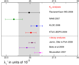
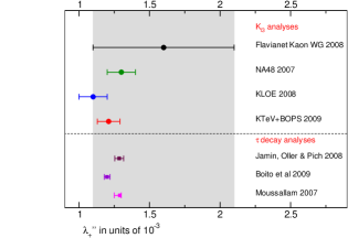
Figure 1: Results on $\lambda^{\prime}_{+}$ (left) and $\lambda^{\prime\prime}_{+}$ (right) from the dispersive analyses of the $K_{\ell 3}$ decays [25, 27, 23] compared to the average of quadratic/linear analyses from the Flavianet Kaon Working Group (WG) [38] and to the results from $\tau\rightarrow K\pi\nu_{\tau}$ analyses [41, 42, 43].

(quadratic/linear analysis) from the Flavianet Kaon Working Group (WG) [38] are also represented. It can be seen that for the vector form factor the results of the dispersive analyses of KLOE, KTeV and NA48 agree reasonably well for $\lambda^{\prime}_{+}$ and very well for $\lambda^{\prime\prime}_{+}$. The dispersive analyses improve very much on the precision of the measured slope and curvature compared to the previous quadratic/linear ones; especially the result on the curvature is improved by a factor 4 compared to the average of the quadratic/linear fits. The vector form factor can also be determined from studies of $\tau\rightarrow K\pi\nu_{\tau}$ decays using the recent data from Belle [39] and BaBar [40]. The results using Belle data are shown in Fig.1. To describe the $\tau$ decays, one needs to know the phase of the vector form factor at higher energy than for the $K_{\ell 3}$ decay fits. To determine it in the inelastic region, one has thus to rely on models. For instance, in Refs. [41, 42] the inelastic effects have been neglected and two resonances have been included and in Ref. [43] a coupled-channel analysis has been performed. As can be seen from Fig.1, there is a very good agreement with the $K_{\ell 3}$ analyses for both determination of the slope and curvature with a much smaller uncertainty on the determination of the curvature. A combination of the two analyses, as presented in Ref. [44], can be very interesting to perform in order to have a better determination of the vector form factor parameters and to test the correlation between slope and curvature imposed by the dispersion relation used in the $K_{\ell 3}$ analyses.

Experiment	Channel	ln$C$	$r$
KTeV [23]	KLμ3+KLe3	0.192(12)	0.978(14)
KLOE [27]	KLμ3+KLe3	0.204(25)	0.990(26)
NA48 [25]	KLμ3	0.144(14)	0.932(15)
SM		0.2141(73)	1

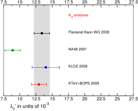
Figure 2: Left: Table, Results on ln$C$ from the dispersive analyses of the $K_{\ell 3}$ decays [25, 27, 23] compared to the SM expectation and extraction of $r$, Eq. (3.6). The SM expectation for ln$C$ is obtained from Eq. (3.4) using $(f_{K}/(f_{\pi}f_{+}(0)))|_{SM}$, Eq. (3.5), and $\Delta_{CT}$, Eq. (2.9), as input values. Right: Results on $\lambda^{\prime}_{0}$ from the dispersive analyses of the $K_{\ell 3}$ decays [25, 27, 23] compared to the average of the quadratic/linear analyses from the Flavianet Kaon WG [38].

As for the determination of the scalar form factor, the results on its slope shown in figure 2 (right) from KLOE and KTeV are in agreement whereas the one from NA48 differs from the others by more than 2 $\sigma$. $\lambda_{0}^{\prime\prime}$ is found to be small, of order $6\cdot 10^{-4}$ but it can’t be neglected to reach a high degree of precision. In principle, a measurement of the scalar form factor is also possible from the lowest energy part of the $\tau\rightarrow K\pi\nu_{\tau}$ decay distribution where it dominates. But, at present, the precision at threshold is not high enough to allow for a competitive determination of the scalar form factor parameters from this decay. A measurement of $\bar{f}_{0}(t)$ from $\tau\rightarrow K\pi\nu_{\tau}$ decays with a good precision will certainly be possible in the near future thanks to new measurements, see for example Ref. [45]. Moreover $K^{+}$ measurements from NA48 and KLOE are underway which might help to solve the puzzle on the scalar form factor measurement.

2.1.4 Determination of $f_{+}(0)$

Using the theoretical inputs described before and the most recent experimental data [38], from Eq. (1), one gets as an average on the neutral and charged modes [46]

$$|f_{+}(0)V_{us}|=0.2163(5)~{}.$$ (12)

To determine $|V_{us}|$, one has to calculate the hadronic key quantity $f_{+}(0)$. In the chiral limit and, more generally, in the $SU(3)$ limit ($m_{u}=m_{d}=m_{s}$) the conservation of the vector current (CVC) implies $f_{+}(0)$=1. Expanding around the chiral limit in powers of light quark masses we can write

$$f_{+}(0)=1+f_{2}+f_{4}+\ldots,$$ (13)

where $f_{n}=\mathcal{O}\left(m_{u,d,s}^{n}/(4\pi f_{\pi})^{n}\right)$, $f_{2}$ and $f_{4}$ being the NLO and NNLO corrections in ChPT. The Ademollo-Gatto theorem [47] implies that $[f_{+}(0)-1]$ is at least of second order in the breaking of $SU(3)$ so that $f_{2}$ is free of any LECs. It can therefore be computed with high accuracy: $f_{2}=-0.0227$ [10, 48]. The difficulty is then in the calculation of the quantity $\Delta f$

$$\Delta f\equiv f_{4}+f_{6}+\ldots=f_{+}(0)-(1+f_{2})~{},$$ (14)

which depends on some LECs. The original estimate based on quark model from Leutwyler and Roos (LR) [48] gives $\Delta f=-0.016(8)$ and $f_{+}(0)=0.961(8)$. Then more recently some analytical calculations have been performed to evaluate the NNLO term $f_{4}$ writing it as

$$f_{4}=\Delta(\mu)+f_{4}|^{\rm loc}(\mu)\,,$$ (15)

where $\Delta(\mu)$ is the loop contribution, $\mu$ being the renormalization scale which has been computed in Ref. [49], and $f_{4}|^{\rm loc}(\mu)$ is the $\mathcal{O}(p^{6})$ local contribution which contains unknown $\mathcal{O}(p^{4})$ and $\mathcal{O}(p^{6})$ LECs. To estimate the latter term various models have been used namely a quark model [49], dispersion relations [50] or $1/N_{C}$ estimates [51]. These calculations allow for a better control of the systematic uncertainties. The values obtained are summarized in Fig.3 (left). They are significantly larger than the LR estimate leading to smaller $SU(3)$ breaking effects on $f_{+}(0)$.

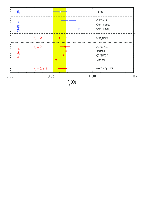
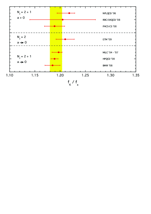
Figure 3: Left: Present determinations of $f_{+}(0)\equiv f_{+}^{K^{0}\pi^{-}}(0)$ in blue from analytical or semi-analytical approaches [48, 49, 50, 51, 12] compared to the ones in red from lattice QCD [53, 54, 56, 57, 58]. Right: $f_{K}/f_{\pi}$ from lattice QCD calculations [62, 63, 64, 65, 66, 67, 68, 69]. The yellow bands correspond to average values given in [60, 59] and $N_{f}$ denotes the number of dynamical quarks. Figures courtesy of S. Simula.

Note that in principle the NNLO term $f_{4}$ may be obtained from the measurement of the slope and the curvature of the scalar form factor $f_{0}(t)$ [49, 34]. The present level of precision coming from the $K_{L\mu 3}$ measurements as well as the knowledge of the $\mathcal{O}(p^{4})$ LECs entering the calculation limit the precision of the extraction. The procedure of averaging the scalar form factor parameters within the Flavianet kaon working group as well as the update of the determination of the $\mathcal{O}(p^{4})$ LECs [52] should improve on the precision of this determination in the near future.

As it was discussed at this conference, lattice calculations give very precise results for $f_{+}(0)$, up to the level of $0.5\%$ as shown in Fig.3 (left). They are in agreement with the result from the pioneering work of LR [48] but give larger $SU(3)$ breaking compared to the recent analytical estimates. This is essentially due to the large positive two loop contribution [49]. Note that only one calculation for $f_{+}(0)$ in $N_{f}=2+1$ flavours exists. Using this result [58] leads to [46], $|V_{us}|=0.2243(12)$, which is at the moment the most precise extraction of $|V_{us}|$.

2.2 $K_{\ell 2}/\pi_{\ell 2}$ ratio of decay rates

Another possibility to extract $|V_{us}|$ is to use the photon inclusive $K_{\ell 2}/\pi_{\ell 2}$ ratio of decay rates written as [2]

$$\frac{\Gamma_{K^{\pm}_{\ell 2(\gamma)}}}{\Gamma_{\pi^{\pm}_{\ell 2(\gamma)}}}=\left|\frac{V_{us}}{V_{ud}}\right|^{2}\frac{f^{2}_{K}M_{K}}{f^{2}_{\pi}M_{\pi}}\left(\frac{1-m^{2}_{\ell}/M_{K}^{2}}{1-m^{2}_{\ell}/M_{\pi}^{2}}\right)^{2}~{}\left(1+\delta_{\rm em}\right),$$ (16)

where $\delta_{\rm em}$ stands for the long-distance electromagnetic (EM) corrections and depends on the hadronic structure and the particle masses as well as on the electromagnetic radiative corrections. For more details on its calculation, see Ref. [2]. By taking the ratio, $\Gamma_{K^{\pm}_{\ell 2(\gamma)}}/\Gamma_{\pi^{\pm}_{\ell 2(\gamma)}}$, Eq. (16), all the channel-independent corrections cancel allowing to estimate the EM corrections with a good precision, $\delta_{\rm em}=-0.0070(35)$ [61]. Hence from the experimental measurements of the ratio of decay rates $\Gamma_{K^{\pm}_{\ell 2(\gamma)}}/\Gamma_{\pi^{\pm}_{\ell 2(\gamma)}}$, one can extract [60]

$$\frac{f^{2}_{K}}{f^{2}_{\pi}}\left|\frac{V_{us}}{V_{ud}}\right|^{2}=0.2758\pm 0.0007~{}.$$ (17)

To access $|V_{us}|/|V_{ud}|$, one needs to know the ratio of the kaon versus pion decay constants $f_{K}/f_{\pi}$. The analytic evaluation of this ratio within ChPT depends already at order $\mathcal{O}(p^{4})$ on the determination of some LECs and thus bring additional uncertainties. This is why the most precise evaluations come from lattice QCD calculations.

The status of the lattice results for $f_{K}/f_{\pi}$ is summarized in Fig.3 (right). The agreement between the different results is remarkable and the present overall accuracy is very good being of about $1\%$. For discussions and details on the lattice set-ups and results, we refer to the forthcoming review by the Flavianet Lattice Averaging Group (FLAG) presented at this conference by G. Colangelo [59] and also to the talk by P. Boyle [70]. As presented in Ref. [71], taking for illustrative purpose the HPQCD-UKQCD result [65], one gets $|V_{us}|/|V_{ud}|=0.2319(15)$.

3 Applications: Stringent tests of the Standard Model

3.1 Determination of $|V_{us}|$ and the CKM unitarity test

Combining the result on $|V_{us}|$ from $K_{\ell 3}$ decays, with the one on $|V_{us}|/|V_{ud}|$ from the $K_{\ell 2}/\pi_{\ell 2}$ ratio of decay rates and the one on $|V_{ud}|$ from superallowed $\beta$ decays [76] in a global fit allows to improve on the precision of the determination of $|V_{us}|$ and to perform a very precise test of the CKM unitarity (test of unitarity of the first row of the CKM matrix) which leads to stringent constraints on new physics scenarios [38, 72, 73], see the talk by M. Palutan [71].

3.2 Test of lepton universality and extraction of the quark mass ratio using $K_{\ell 3}$ decays

The precision reached in the measurements of the $K_{\ell 3}$ decays [38] and in the determination of the EM corrections, see section 2.1.1, allows for putting very interesting constraints on lepton universality and also for a precise extraction of the quark mass ratios, $Q$ and $R$. Concerning the test of lepton universality, using Eq. (1), one can determine the ratio

$$r_{\mu/e}=\frac{G_{\mu}^{2}}{G_{e}^{2}}=\frac{\Gamma_{K_{\mu 3}}}{\Gamma_{K_{e3}}}\frac{I_{K}^{e}}{I_{K}^{\mu}}(1+2\Delta_{\rm EM}^{Ke}-2\Delta_{\rm EM}^{K\mu})~{}.$$ (18)

Averaging charged and neutral modes, one gets $r_{\mu/e}=1.002\pm 0.005$ [46] consistent with lepton universality. With an accuracy of $0.5\%$, this determination becomes by now competitive with other determinations such as the one coming from $\tau$ decays, see Ref. [71].

In addition, a phenomenological determination of $\Delta_{\rm SU(2)}^{K\pi}$, see section 2.1.2, is by now possible comparing the results on charged and neutral decay widths, Eq. (1). One obtains [38, 71]

$$\Delta_{\rm SU(2)}^{K\pi}=\frac{\Gamma_{K^{+}_{\ell 3}}}{\Gamma_{K^{0}_{\ell 3}}}\frac{I_{K^{0}}^{\ell}}{I_{K^{+}}^{\ell}}\left(\frac{M_{K^{0}}}{M_{K^{+}}}\right)^{5}-\frac{1}{2}-[\Delta^{K^{+}\ell}_{\rm EM}-\Delta^{K^{0}\ell}_{\rm EM}]=2.7(4)\%$$ (19)

in good agreement with the value of Eq. (6), favouring a small value for R

$$R=33.2\pm 4.7~{}.$$ (20)

3.3 Test of the SM electroweak couplings via the CT theorem with $K_{\ell 3}$ and $K_{\ell 2}$ decays

Among the possible tests of the Standard Model and the new physics scenarios using $K_{\ell 3}$ and $K_{\ell 2}$ decays, the Callan-Treiman theorem, Eq. (8), offers a very stringent test of the SM electroweak (EW) couplings due to the small size of $\Delta_{CT}$, Eq. (9). The test consists of comparing the value of $f_{K}/(f_{\pi}~{}f_{+}(0))$ deduced from the measurement of C from the $K_{\mu 3}$ dispersive analyses using the Callan-Treiman theorem rewritten as

$$\frac{f_{K}}{f_{\pi}f_{+}(0)}=C-\Delta_{CT}~{},$$ (21)

to the value of $f_{K}/(f_{\pi}~{}f_{+}(0))|_{SM}$ determined by assuming the SM EW couplings and using the experimental measurements of $\Gamma_{K^{+}_{\ell 2(\gamma)}}/\Gamma_{\pi^{+}_{\ell 2(\gamma)}}$, Eq. (16) [60], of $\Gamma_{K_{Le3(\gamma)}}$, Eq. (1), (from the electronic neutral mode) [46] and the value of $|V_{ud}|$ [76]. One gets

$$\frac{f_{K}}{f_{\pi}f_{+}(0)}|_{SM}=a~{}\left(\frac{\Gamma_{K^{\pm}_{\ell 2(\gamma)}}}{\Gamma_{\pi^{\pm}_{\ell 2(\gamma)}}}~{}\frac{1}{\Gamma_{K_{Le3(\gamma)}}}\right)^{1/2}~{}|V_{ud}|=1.2422\pm 0.0043~{},$$ (22)

with $a$, a constant determined from the theoretical inputs, see Eqs. (1) and (16). If the two values differ that means if

$$r\equiv(C-\Delta_{CT})\cdot\frac{f_{\pi}f_{+}(0)}{f_{K}}|_{SM}$$ (23)

is different from one, that would indicate the presence of new physics such as modification of EW couplings of quarks due to exchanges of new particles close to the TeV scale. This can be, for instance, due to a direct coupling of right-handed quarks to the W-boson which appears at NLO of an Higgsless low-energy effective theory [35, 77] or to couplings of quarks to a charged Higgs. Hence the CT theorem can be used to constrain the masses and the couplings of the new particles appearing in such scenarios, see e.g. Refs. [35, 38, 71, 78] for further discussions. The results from the different analyses are reported in the table Fig.2 (left) for ln$C$, the logarithm of $C$, Eq. (21) and for $r$, Eq. (23). The result of NA48 doesn’t agree with the ones from KTeV and KLOE which are consistent with the SM expectation. It disagrees with the SM at $4.5\sigma$ indicating, if confirmed, presence of physics beyond the SM. An effect at the level of several percents would be, however, difficult to accommodate in a charged Higgs scenario where the effects for natural values of the parameters are expected at the per mile level, whereas in the Higgless case, that would indicate an inverted hierarchy for the right-handed mixing matrix $V_{R}$. As mentioned already, some measurements especially for the charged modes are underway to try to solve this puzzle.

4 Lepton universality test via $R_{K}$

Let me briefly mention a particularly sensitive probe of new physics given by the universality ratio

$$R_{K}^{e/\mu}=\frac{\Gamma_{K_{e2(\gamma)}}}{\Gamma_{K_{\mu 2(\gamma)}}}~{}.$$ (24)

This quantity is helicity suppressed in the SM as a consequence of the $V-A$ structure of the charged currents and thus is very small. Moreover it has been calculated with a very high level of accuracy recently [74] in a first systematic calculation to $e^{2}p^{2}$ leading to

$$R_{K}^{e/\mu}=(2.477\pm 0.001)\times 10^{-5}~{}.$$ (25)

The uncertainty is at the level of 0.04 $\%$ mainly due to the fact that to a first approximation many contributions such as the hadronic ones cancel out by taking the ratio. The hadronic structure dependence only appears through EW corrections. So one has only to evaluate the diagrams with photons connected to lepton lines. The relevant counterterms are estimated by a matching with large $N_{C}$ QCD. In this work, the real photon corrections have been included and the leading logarithms have been resumed. The previous calculation of Ref. [75] has been improved. However a discrepancy at $5\sigma$ exists between the two results but can be traced back to inconsistencies in the previous analysis.

Measuring this ratio is very interesting since it has been shown that in realistic supersymmetric frameworks with new sources of lepton flavour mixings, deviations from the SM can reach the level of $1\%$ [79]. Since the conference Kaon’07 there have been very impressive experimental improvements in the measurement of this quantity as presented at this conference [81, 82]. The world average from March 2009 [80] is

$$R_{K}^{e/\mu}=(2.468\pm 0.025)\times 10^{-5}~{},$$ (26)

confirming the SM expectation, Eq. (25). There is still room for improvements on the experimental side which could be achieved thanks to the NA62 experiment [82].

5 Conclusion

The charged current analyses using $K_{\ell 3}$ and $K_{\ell 2}$ data have entered an area of very high precision. On the theoretical side, a lot of work has been performed within the last years to improve on the precision of the determination of the electromagnetic and isospin breaking corrections. Moreover dedicated dispersive parametrizations to analyse the $K_{\ell 3}$ form factors with a high level of accuracy have been built. A lot of progress has also been done experimentally, see Ref. [71]. This allows for very precise tests of the SM such as the CKM unitarity test or lepton flavour violation ones and gives interesting constraints on new physics scenarios. One should notice that in order to improve on the SM tests, especially on the one using the CT theorem, one would need to improve on the scalar form factor measurements and in particular on the charged channel where only one recent measurement has been performed [28]. This would also allow for a better precision on the extraction of the quark mass ratio $R$. On the theoretical side, the determination of $f_{+}(0)$ should be improved. Indeed, the lattice determinations don’t agree well with the analytical results and there is only one $N_{f}=2+1$ flavours result. In this respect, the recent progress in lattice calculations are promising.

Acknowledgments

I would like to thank the organizers for their invitation and for this very pleasant and interesting conference. This work has been supported in part by the EU contract MRTN-CT-2006-035482 (”Flavianet”).

References

- [1] A. Sirlin, Rev. Mod. Phys. 50 (1978) 573 [Erratum-ibid. 50 (1978) 905]; A. Sirlin, Nucl. Phys. B 196 (1982) 83.
- [2] W. J. Marciano and A. Sirlin, Phys. Rev. Lett. 71 (1993) 3629.
- [3] E. S. Ginsberg, Phys. Rev. 142, 1035 (1966).
- [4] V. Bytev, E. Kuraev, A. Baratt and J. Thompson, Eur. Phys. J. C 27 (2003) 57 [Erratum-ibid. C 34 (2004) 523] [arXiv:hep-ph/0210049].
- [5] T. C. Andre, Annals Phys. 322 (2007) 2518 [arXiv:hep-ph/0406006].
- [6] V. Cirigliano, M. Knecht, H. Neufeld, H. Rupertsberger and P. Talavera, Eur. Phys. J. C 23, 121 (2002) [arXiv:hep-ph/0110153]; V. Cirigliano, H. Neufeld and H. Pichl, Eur. Phys. J. C 35, 53 (2004) [arXiv:hep-ph/0401173].
- [7] V. Cirigliano, M. Giannotti and H. Neufeld, JHEP 0811 (2008) 006 [arXiv:0807.4507 [hep-ph]].
- [8] B. Ananthanarayan and B. Moussallam, JHEP 0406 (2004) 047 [arXiv:hep-ph/0405206].
- [9] S. Descotes-Genon and B. Moussallam, Eur. Phys. J. C 42 (2005) 403 [arXiv:hep-ph/0505077].
- [10] J. Gasser and H. Leutwyler, Nucl. Phys. B 250 (1985) 517.
- [11] V. Cirigliano, PoS KAON (2008) 007.
- [12] A. Kastner and H. Neufeld, Eur. Phys. J. C 57 (2008) 541 [arXiv:0805.2222 [hep-ph]].
- [13] R. F. Dashen, Phys. Rev. 183 (1969) 1245.
- [14] J. Kambor, C. Wiesendanger and D. Wyler, Nucl. Phys. B 465 (1996) 215 [arXiv:hep-ph/9509374].
- [15] A. V. Anisovich and H. Leutwyler, Phys. Lett. B 375 (1996) 335 [arXiv:hep-ph/9601237]; H. Leutwyler, Phys. Lett. B 378 (1996) 313 [arXiv:hep-ph/9602366].
- [16] J. Bijnens and K. Ghorbani, JHEP 0711 (2007) 030 [arXiv:0709.0230 [hep-ph]].
- [17] F. Ambrosino et al. [KLOE Collaboration], JHEP 0805 (2008) 006 [arXiv:0801.2642 [hep-ex]].
- [18] G. Colangelo, S. Lanz and E. Passemar, PoS CD09 (2009) 047, [arXiv:0910.0765 [hep-ph]].
- [19] K. Kampf, M. Knecht, J. Novotny and M. Zdrahal, work in progress.
- [20] H. Leutwyler, PoS CD09 (2009) 005 [arXiv:0911.1416 [hep-ph].
- [21] A. Bazavov et al. [The MILC Collaboration], PoS CD09 (2009) 007 [arXiv:0910.2966 [hep-ph]].
- [22] T. Alexopoulos et al. [KTeV Collaboration], Phys. Rev. D 70 (2004) 092007 [arXiv:hep-ex/0406003]; E. Abouzaid et al. [KTeV Collaboration], Phys. Rev. D 74, 097101 (2006) [arXiv:hep-ex/0608058].
- [23] E. Abouzaid et al. [KTeV collaboration], arXiv:0912.1291 [hep-ex], to be published in Phys. Rev. D.
- [24] A. Lai et al. A. Lai et al. [NA48 Collaboration], Phys. Lett. B 604 (2004) 1 [arXiv:hep-ex/0410065].
- [25] A. Lai et al. [NA48 Collaboration], Phys. Lett. B 647 (2007) 341 [arXiv:hep-ex/0703002].
- [26] F. Ambrosino et al. [KLOE Collaboration], Phys. Lett. B 636 (2006) 166 [arXiv:hep-ex/0601038].
- [27] F. Ambrosino et al. [KLOE Collaboration], JHEP 0712 (2007) 105 [arXiv:0710.4470 [hep-ex]].
- [28] O. P. Yushchenko et al., Phys. Lett. B 581 (2004) 31 [arXiv:hep-ex/0312004]; O. P. Yushchenko et al., Phys. Lett. B 589 (2004) 111 [arXiv:hep-ex/0404030].
- [29] R. J. Hill, Phys. Rev. D 74 (2006) 096006 [arXiv:hep-ph/0607108].
- [30] G. Abbas and B. Ananthanarayan, Eur. Phys. J. A 41, 7 (2009) [arXiv:0905.0951 [hep-ph]]; G. Abbas, B. Ananthanarayan, I. Caprini, I. S. Imsong and S. Ramanan, arXiv:0912.2831 [hep-ph].
- [31] C. G. Callan and S. B. Treiman, Phys. Rev. Lett. 16 (1966) 153; R. F. Dashen and M. Weinstein, Phys. Rev. Lett. 22 (1969) 1337.
- [32] H. Leutwyler, private communication.
- [33] J. Bijnens and K. Ghorbani, arXiv:0711.0148 [hep-ph].
- [34] V. Bernard and E. Passemar, Phys. Lett. B 661 (2008) 95 [arXiv:0711.3450 [hep-ph]].
- [35] V. Bernard, M. Oertel, E. Passemar and J. Stern, Phys. Lett. B 638 (2006) 480 [arXiv:hep-ph/0603202].
- [36] K. M. Watson, Phys. Rev. 88, 1163 (1952).
- [37] V. Bernard, M. Oertel, E. Passemar and J. Stern, Phys. Rev. D 80 (2009) 034034 [arXiv:0903.1654 [hep-ph]].
- [38] M. Antonelli et al. [FlaviaNet Working Group on Kaon Decays], arXiv:0801.1817 [hep-ph].
- [39] D. Epifanov et al. [Belle Collaboration], Phys. Lett. B 654 (2007) 65 [arXiv:0706.2231 [hep-ex]].
- [40] B. Aubert et al. [BABAR Collaboration], Phys. Rev. D 76 (2007) 051104 [arXiv:0707.2922 [hep-ex]]; B. Aubert et al., talk presented at ICHEP08, Philadelphia, Pennsylvania, [arXiv:0808.1121 [hep-ex]].
- [41] M. Jamin, A. Pich and J. Portoles, Phys. Lett. B 640 (2006) 176 [arXiv:hep-ph/0605096]; ibid, Phys. Lett. B 664 (2008) 78 [arXiv:0803.1786 [hep-ph]].
- [42] D. R. Boito, R. Escribano and M. Jamin, Eur. Phys. J. C 59 (2009) 821 [arXiv:0807.4883 [hep-ph]].
- [43] B. Moussallam, Eur. Phys. J. C 53 (2008) 401 [arXiv:0710.0548 [hep-ph]].
- [44] D. R. Boito, R. Escribano and M. Jamin, PoS EFT09, 064 (2009) [arXiv:0904.0425 [hep-ph]].
- [45] S. Paramesvaran and f. t. B. Collaboration, arXiv:0910.2884 [hep-ex].
- [46] M. Moulson, Talk given at WIN09, Perugia, Italy, - September 2009.
- [47] M. Ademollo and R. Gatto, Phys. Rev. Lett. 13 (1964) 264.
- [48] H. Leutwyler and M. Roos, Z. Phys. C 25 (1984) 91.
- [49] J. Bijnens and P. Talavera, Nucl. Phys. B 669 (2003) 341 [arXiv:hep-ph/0303103].
- [50] M. Jamin, J. A. Oller and A. Pich, JHEP 0402 (2004) 047 [arXiv:hep-ph/0401080].
- [51] V. Cirigliano, G. Ecker, M. Eidemuller, R. Kaiser, A. Pich and J. Portoles, JHEP 0504 (2005) 006 [arXiv:hep-ph/0503108].
- [52] J. Bijnens and I. Jemos, PoS(CD09)087 arXiv:0909.4477 [hep-ph].
- [53] D. Becirevic et al., Nucl. Phys. B 705 (2005) 339 [arXiv:hep-ph/0403217].
- [54] N. Tsutsui et al. [JLQCD Collaboration], PoS LAT2005 (2006) 357 [arXiv:hep-lat/0510068].
- [55] C. Dawson, T. Izubuchi, T. Kaneko, S. Sasaki and A. Soni, Phys. Rev. D 74 (2006) 114502 [arXiv:hep-ph/0607162].
- [56] D. Brommel et al. [The QCDSF collaboration], PoS LAT2007 (2007) 364 [arXiv:0710.2100 [hep-lat]].
- [57] V. Lubicz, F. Mescia, S. Simula, C. Tarantino and f. t. E. Collaboration, Phys. Rev. D 80 (2009) 111502 [arXiv:0906.4728 [hep-lat]]; F. Mescia, these proceedings, PoS KAON09 (2009) 028.
- [58] P. A. Boyle et al., Phys. Rev. Lett. 100 (2008) 141601 [arXiv:0710.5136 [hep-lat]].
- [59] G. Colangelo, these proceedings, PoS KAON09 (2009) 029; The FLAVIAnet Lattice Averaging Group (FLAG), in preparation.
- [60] M. Antonelli et al., arXiv:0907.5386 [hep-ph].
- [61] W. J. Marciano, Phys. Rev. Lett. 93 (2004) 231803 [arXiv:hep-ph/0402299].
- [62] B. Blossier et al., JHEP 0907 (2009) 043 [arXiv:0904.0954 [hep-lat]].
- [63] C. Aubin et al. [MILC Collaboration], Phys. Rev. D 70 (2004) 114501 [arXiv:hep-lat/0407028]; C. Bernard et al., PoS LAT2007 (2007) 090 [arXiv:0710.1118 [hep-lat]].
- [64] S. R. Beane, P. F. Bedaque, K. Orginos and M. J. Savage, Phys. Rev. D 75 (2007) 094501 [arXiv:hep-lat/0606023].
- [65] E. Follana, C. T. H. Davies, G. P. Lepage and J. Shigemitsu [HPQCD Collaboration and UKQCD Collaboration], Phys. Rev. Lett. 100 (2008) 062002 [arXiv:0706.1726 [hep-lat]].
- [66] C. Allton et al. [RBC-UKQCD Collaboration], Phys. Rev. D 78 (2008) 114509 [arXiv:0804.0473 [hep-lat]].
- [67] S. Aoki et al. [PACS-CS Collaboration], arXiv:0807.1661 [hep-lat].
- [68] C. Aubin, J. Laiho and R. S. Van de Water, arXiv:0810.4328 [hep-lat].
- [69] S. Dürr, talk at The XXVI International Symposium on Lattice Field Theory, 2008.
- [70] P. A. Boyle, these proceedings, PoS KAON09 (2009) 002 [arXiv:0911.4317 [hep-ph]].
- [71] M. Palutan, these prooceedings, PoS KAON09 (2009) 008.
- [72] W. J. Marciano, PoS KAON (2008) 003.
- [73] V. Cirigliano, J. Jenkins and M. Gonzalez-Alonso, arXiv:0908.1754 [hep-ph].
- [74] V. Cirigliano and I. Rosell, Phys. Rev. Lett. 99 (2007) 231801 [arXiv:0707.3439 [hep-ph]]; V. Cirigliano and I. Rosell, JHEP 0710 (2007) 005 [arXiv:0707.4464 [hep-ph]].
- [75] M. Finkemeier, Phys. Lett. B 387 (1996) 391 [arXiv:hep-ph/9505434].
- [76] J. C. Hardy and I. S. Towner, Phys. Rev. C 79 (2009) 055502 [arXiv:0812.1202 [nucl-ex]].
- [77] V. Bernard, M. Oertel, E. Passemar and J. Stern, JHEP 0801 (2008) 015 [arXiv:0707.4194 [hep-ph]].
- [78] O. Deschamps et al. arXiv:0907.5135 [hep-ph].
- [79] A. Masiero, P. Paradisi and R. Petronzio, Phys. Rev. D 74 (2006) 011701 [arXiv:hep-ph/0511289]; ibid, JHEP 0811 (2008) 042 [arXiv:0807.4721 [hep-ph]]; P. Paradisi, these proceedings, PoS KAON09 (2009) 044.
- [80] T. Spadaro [KLOE collaboration], arXiv:0907.2613 [hep-ex].
- [81] B. Sciascia [KLOE Collaboration], these proceedings, PoS KAON09 (2009) 025 [arXiv:0908.4584 [hep-ex]].
- [82] E. Goudzovski, these proceedings, PoS KAON09 (2009) 026.