Identification of Convection Heat Transfer Coefficient
of Secondary Cooling Zone of CCM
based on Least Squares Method and Stochastic Approximation Method

Abstract

The detailed mathematical model of heat and mass transfer of steel ingot of curvilinear continuous casting machine is proposed. The process of heat and mass transfer is described by nonlinear partial differential equations of parabolic type. Position of phase boundary is determined by Stefan conditions. The temperature of cooling water in mould channel is described by a special balance equation. Boundary conditions of secondary cooling zone include radiant and convective components of heat exchange and account for the complex mechanism of heat-conducting due to airmist cooling using compressed air and water. Convective heat-transfer coefficient of secondary cooling zone is unknown and considered as distributed parameter. To solve this problem the algorithm of initial adjustment of parameter and the algorithm of operative adjustment are developed.

1 Introduction

Improved computing significantly increased role of mathematical modeling in research of thermo-physical processes. This, in turn, imposes stricter requirements towards accuracy and efficiency of mathematical models.

It is well known that successful modeling mostly depends on the right choice of a model, which is directly affected by reliability of thermo-physical parameters used. Frequently, empirical data alone can not provide sufficient information about one-valuedness conditions.

Therefore recently the big attention is given to the solution of inverse problems of heat conduction, in which it is necessary to define thermophysical properties of an object on available (frequently rather limited) information about temperature field. In particular thus it is possible to identify boundary conditions. There are difficulties in choice of some parameters of process for development of mathematical models of technological processes.

While modeling process for specific industrial conditions it is necessary to determine some thermal or physical parameters each time, in particular convective heat-transfer coefficient (CHTC) on a surface of an ingot in the secondary cooling zone which depends on many factors. It is connected by that the convective heat transfer coefficient value is influenced with set of various factors. Besides, CHTC value can vary strongly enough in a time and on space coordinates. Thus, there is a problem of identification of the CHTC as distributed parameter.

In the given work algorithms of initial adjustment of parameter when at the disposal of there is enough plenty of points in which the temperature on a surface of an ingot is measured, and operative adjustment when the temperature is measured only in one point on a surface are considered.

2 Statement of problem

The thermal field of the moving steel ingot and mold wall in the system of coordinates attached to motionless construction of CCM is considered [1]. In fig. 1 the diagram of CCM is introduced.

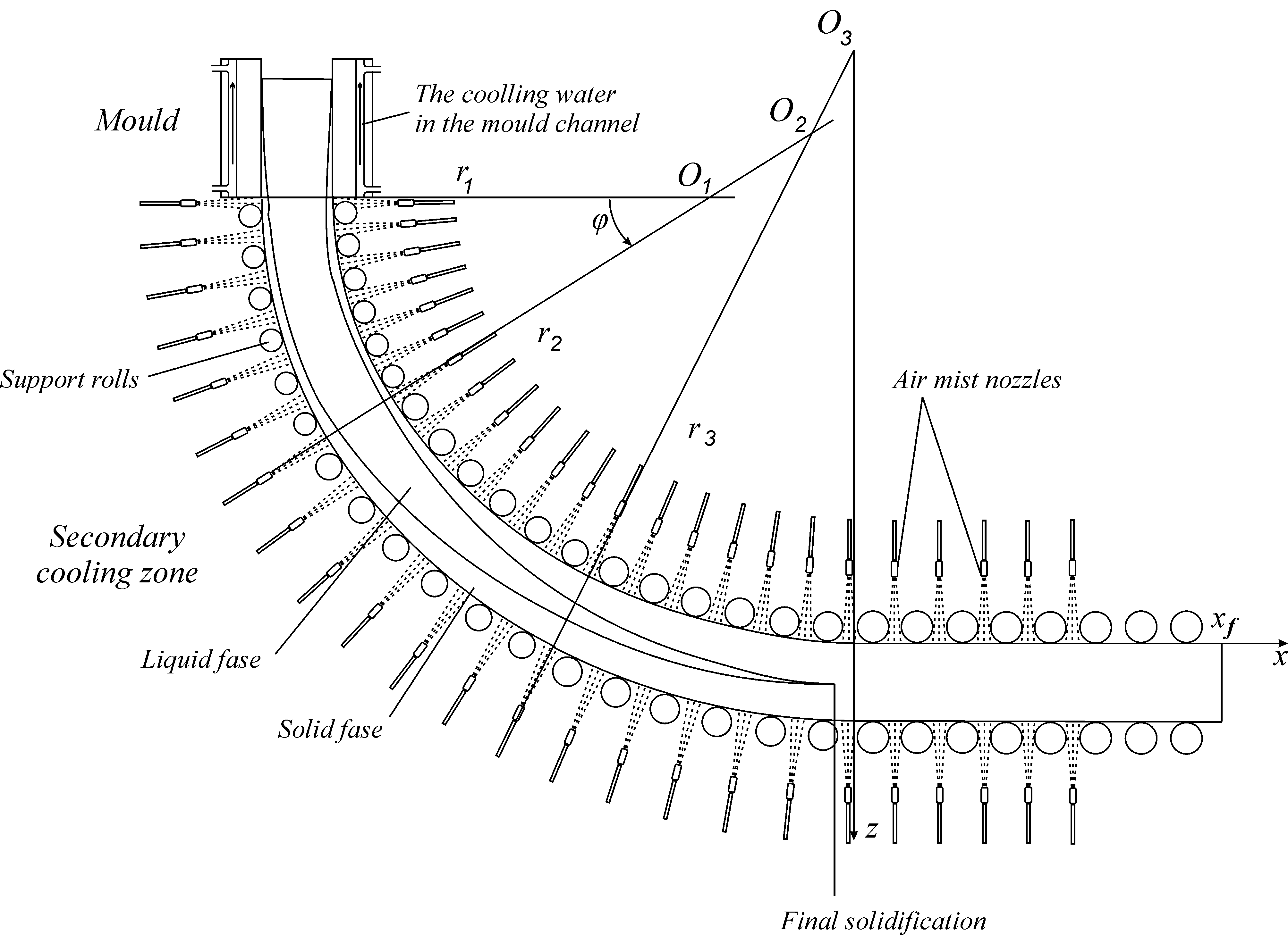
Figure 1:

The heat conduction in the steel ingot in the mold area is described by nonstationary, nonlinear heat and mass transfer equation:

$$\begin{array}[]{l}{\displaystyle\frac{\partial T(\tau,x,z)}{\partial\tau}+v(\tau)\frac{\partial T\left({\tau,x,z}\right)}{\partial z}=}\\ \\ {\displaystyle=\frac{1}{c(T,x,z)\rho(T,x,z)}\left\{{\frac{\partial}{\partial x}\left[{\lambda(T,x,z)\frac{\partial T}{\partial x}}\right]+\frac{\partial}{\partial z}\left[{\lambda(T,x,z)\frac{\partial T}{\partial z}}\right]}\right\},}\\ \\ {\displaystyle\ \qquad\qquad\qquad\qquad\qquad 0<x<l,\quad 0<z<Z}\end{array}$$

and the boundary conditions:

$$\begin{array}[]{c}{\displaystyle\ -\lambda(T,x)\frac{\partial T}{\partial z}=0,\quad 0\leq x\leq l,}\\ \\ {\displaystyle\ \left.{\frac{\partial T}{\partial x}}\right|_{x=0}=0,\quad 0\leq z\leq Z,}\\ \\ {\displaystyle\ \lambda(T,z)\left.{\frac{\partial T}{\partial x}}\right|_{x=l}=\frac{\lambda_{gz}}{\delta}\left({\left.T\right|_{x=l+\delta}-\left.T\right|_{x=l}}\right)+\sigma_{n}\left[{\left({\frac{\left.T\right|_{x=l+\delta}}{100}}\right)^{4}-\left({\frac{\left.T\right|_{x=l}}{100}}\right)^{4}}\right],}\\ \\ \quad 0\leq z\leq Z,\end{array}$$

where $v(\tau)$ – withdrawal rate, $2l$ – ingot thickness, $Z$ – height of ingot in the mould, $T(\tau,x,z)$ – metal temperature, $c(T,x,z)$ – metal specific heat, $\rho(T,x,z)$ – density, $\lambda(T,x,z)$ – thermal conduction, $\delta\leavevmode\nobreak\$ – effective thickness of air gap between ingot and the mould wall, $\lambda_{gz}$ – thermal conduction coefficient of gap gas mixture, $\left.T\right|_{x=l}$ – surface temperature of the ingot, $\left.T\right|_{x=l+\delta}$ – surface temperature of mold wall, $\sigma_{n}$ – the resulted radiation coefficient.

Conditions of equality of temperatures and Stefan conditions, and also boundary and initial conditions for the phase boundary are set:

$$\begin{array}[]{c}{\displaystyle\ T\left.{(\tau,x,z)}\right|_{x=\xi_{-}(\tau,z)}=\left.{T(\tau,x,z)}\right|_{x=\xi_{+}(\tau,z)}=T_{kr},}\\ \\ {\displaystyle\ \left.{\lambda(T,x,z)\frac{\partial T}{\partial\bar{n}}}\right|_{x=\xi_{-}(\tau,z)}-\left.{\lambda(T,x,z)\frac{\partial T}{\partial\bar{n}}}\right|_{x=\xi_{+}(\tau,z)}=\mu\rho(T_{kr})\left({\frac{\partial\xi}{\partial\tau}+v\cdot\frac{\partial\xi}{\partial z}}\right),}\\ \\ {\displaystyle\ \quad 0\leq z\leq Z,}\\ \\ {\displaystyle\ \xi(\tau,0)=l,\quad\xi(0,z)=\xi_{0}(z),}\end{array}$$

where $\xi$ – the phase boundary function of two variables $x=\xi(\tau,z)$, $\mu$ – crystallization latent heat, $T_{kr}$ – crystallization temperature (average of the interval “liquidus – solidus”), $\bar{n}$ – normal to the boundary of phases.

Heat equation for mould walls:

$$\begin{array}[]{c}{\displaystyle\ \frac{\partial T(\tau,x,z)}{\partial\tau}=\frac{1}{c(T,x,z)\rho(T,x,z)}\left\{{\frac{\partial}{\partial x}\left[{\lambda(T,x,z)\frac{\partial T}{\partial x}}\right]+\frac{\partial}{\partial z}\left[{\lambda(T,x,z)\frac{\partial T}{\partial z}}\right]}\right\},}\\ \\ {\displaystyle\ z_{0}<z<Z,\quad l<x<d}\end{array}$$

Boundary conditions for mould walls represent the character of heat exchange on each sight of wall:

$$\begin{array}[]{c}{\displaystyle\ \left.{\lambda(T,z)\frac{\partial T}{\partial x}}\right|_{x=d}=\alpha_{1}\left({T_{water}(\tau,z)-\left.T\right|_{x=d}}\right),\quad z_{0}\leq z\leq Z,}\\ \\ {\displaystyle\ \left.{\lambda(T,x)\frac{\partial T}{\partial z}}\right|_{z=Z}=\alpha_{2}\left({T_{os.2}-\left.T\right|_{z=Z}}\right),\quad l\leq x\leq d,\quad z=Z,}\\ \\ {\displaystyle\ -\left.{\lambda(T,x)\frac{\partial T}{\partial z}}\right|_{z=z_{0}}=\alpha_{3}\left({T_{os.3}-\left.T\right|_{z=z_{0}}}\right),\quad l\leq x\leq d,\quad z=z_{0},}\\ \\ {\displaystyle\ \lambda(T,z)\left.{\frac{\partial T}{\partial x}}\right|_{x=l+\delta}=}\\ \\ {\displaystyle\ \qquad\qquad\qquad=\frac{\lambda_{gz}}{\delta}\left({\left.T\right|_{x=l+\delta}-\left.T\right|_{x=l}}\right)+\sigma_{n}\left[{\left({\frac{\left.T\right|_{x=l+\delta}}{100}}\right)^{4}-\left({\frac{\left.T\right|_{x=l}}{100}}\right)^{4}}\right],}\\ \\ \quad 0\leq z\leq Z,\quad x=l+\delta,\\ \\ {\displaystyle\ \left.{-\lambda(T,z)\frac{\partial T}{\partial x}}\right|_{x=l+\delta}=\alpha_{4}\left({T_{os.1}-\left.T\right|_{x=d}}\right)+C_{n}\left[{\left({\frac{T_{os.1}}{100}}\right)^{4}-\left({\frac{\left.T\right|_{x=d}}{100}}\right)^{4}}\right],}\\ \\ \quad z_{0}\leq z\leq 0,\quad x=l+\delta,\end{array}$$

where $d$ – mold wall thickness, $z_{0}$ – mold wall altitude over meniscus level, $\alpha_{1}$ – heat transfer coefficient from the mould wall to cooling water, $T_{water}(\tau,z)$ – cooling water temperature in the mold channel, $\alpha_{2,3,4}$ – heat transfer coefficients from other mould wall to environment, $T_{os.2,3,4}$ – environment temperature, $C_{n}$ – the resulted radiation coefficient.

The following balance equation describes distribution of cooling water temperature in the mold channel:

$$c\cdot S\cdot v_{water}\frac{\partial T_{water}(\tau,z)}{\partial z}=P_{I}\alpha_{1}\left({T_{water}(\tau,z)-\left.T\right|_{x=d}}\right)-P_{E}\alpha_{E}\left({T_{water}(\tau,z)-T_{E}}\right),$$

where $c$ – volume heat capacity of water, $S$ – the cross-section area of the mold channel, $v_{water}$ – water velocity, $P_{I}$ – perimeter of the interior mold wall, $P_{E}$ – perimeter of the external mold wall, $\alpha_{E}$ – heat transfer coefficient from cooling water to the external mould wall, $T_{E}$ – external mould wall temperature.

The cooling water temperature on the entry in the mould channel is known:

$$T_{water}(0,Z)=T_{water1}(\tau)$$

and it’s initial distribution in the mold channel:

$$T_{water}(0,z)=T_{water0}(z)$$

The following equation describes heat and mass transfer on the curvilinear sections of CCM:

$$\begin{array}[]{l}{\displaystyle\ \frac{\partial T}{\partial\tau}+\theta_{m}(\tau)\frac{\partial T(\tau,r,\varphi)}{\partial\varphi}=\frac{1}{c(T,r,\varphi)\rho(T,r,\varphi)}\times}\\ \\ {\displaystyle\ \times\left\{{\frac{\partial}{\partial r}\left({\lambda(T,r,\varphi)\frac{\partial T}{\partial r}}\right)+\frac{1}{r^{2}}\cdot\frac{\partial}{\partial\varphi}\left({\lambda(T,r,\varphi)\frac{\partial T}{\partial\varphi}}\right)+\frac{\lambda(T,r,\varphi)}{r}\cdot\frac{\partial T}{\partial r}}\right\}}\end{array}$$

where $\theta_{m}$ – angular velocity of ingot driving on the $m$-th curvilinear section.

The conditions for unknown boundary on the curvilinear sections are

$$\begin{array}[]{c}{\displaystyle\ \left.{T(\tau,r,\varphi)}\right|_{r=\xi_{1,2-}(\tau,\varphi)}=\left.{T(\tau,r,\varphi)}\right|_{r=\xi_{1,2+}(\tau,\varphi)}=T_{kr},}\\ \\ {\displaystyle\ \left.{\lambda(T,r,\varphi)\frac{\partial T}{\partial\bar{n}}}\right|_{\xi_{1-}}-\lambda(T,r,\varphi)\left.{\frac{\partial T}{\partial\bar{n}}}\right|_{\xi_{1+}}=\mu\rho_{kr}\left({\theta_{m}(\tau)\cdot\frac{\partial\xi_{1}}{\partial\varphi}+\frac{\partial\xi_{1}}{\partial\tau}}\right),}\\ \\ {\displaystyle\ \quad\xi_{1}(0,\varphi)=\xi_{1_{0}}(\varphi),}\\ \\ {\displaystyle\ \lambda(T,r,\varphi)\left.{\frac{\partial T}{\partial\bar{n}}}\right|_{\xi_{2+}}-\lambda(T,r,\varphi)\left.{\frac{\partial T}{\partial\bar{n}}}\right|_{\xi_{2-}}=-\mu\rho_{kr}\left({\theta_{m}(\tau)\cdot\frac{\partial\xi_{2}}{\partial\varphi}+\frac{\partial\xi_{2}}{\partial\tau}}\right),}\\ \\ {\displaystyle\ \quad\xi_{2}(0,\varphi)=\xi_{2_{0}}(\varphi),}\end{array}$$

where $\xi_{1}(\varphi)$ and $\xi_{2}(\varphi)$ – phase boundaries (interfaces).

The boundary conditions of the secondary cooling zone include radiant and convective components of heat exchange and account for the complex mechanism of heat-conducting due to air-mist cooling using compressed air and water. The boundary conditions on the curvilinear sections are

$$\begin{array}[]{l}{\displaystyle\ -\left.{\lambda(T,\varphi)\frac{\partial T}{\partial r}}\right|_{r=r_{m}}=\alpha_{I}(G_{m}(\tau),\varphi)\cdot\left({T_{I_{m}}\left.{-T}\right|_{r=r_{m}}}\right)+C_{I_{m}}\left({T_{I_{m}}^{4}-\left.{(T}\right|_{r=r_{m}})^{4}}\right)}\end{array}$$

$$\begin{array}[]{l}{\displaystyle\ \left.{\lambda(T,\varphi)\frac{\partial T_{2}}{\partial r}}\right|_{r=r_{m}+2l}=}\\ \\ {\displaystyle\ =\alpha_{E}(G_{m}(\tau),\varphi)\cdot\left({T_{E_{m}}-\left.T\right|_{r=r_{m}+2l}}\right)+C_{E_{m}}\left({T_{E_{m}}^{4}-\left.{(T}\right|_{r=r_{m}+2l})^{4}}\right),}\end{array}$$

where $\alpha_{I}(G_{m}(\tau),\varphi)$, $\alpha_{E}(G_{m}(\tau),\varphi)$ – convective heat transfer coefficients, $C_{I_{m}},C_{E_{m}}$ – the resulted radiation coefficients, $T_{I_{m}},T_{E_{m}}$ – environment temperatures, $G_{m}(\tau)$ – water discharge on the $m$-th section.

The following equation describes the heat and mass transfer on rectilinear sections of CCM (analogously (1)):

$$\begin{array}[]{l}{\displaystyle\ \frac{\partial T}{\partial\tau}+v(\tau)\frac{\partial T\left({\tau,x,z}\right)}{\partial x}=}\\ \\ {\displaystyle\ =\frac{1}{c(T,x,z)\rho(T,x,z)}\left\{{\frac{\partial}{\partial x}\left[{\lambda(T,x,z)\frac{\partial T}{\partial x}}\right]+\frac{\partial}{\partial z}\left[{\lambda(T,x,z)\frac{\partial T}{\partial z}}\right]}\right\}}\end{array}$$

When the liquid phase passes the straightening point on the rectilinear section of the secondary cooling zone, the conditions for the unknown phase boundary are set:

$$\begin{array}[]{c}{\displaystyle\ \left.{T(\tau,x,z)}\right|_{x=\xi_{1,2-}(x,z)}=\left.{T(\tau,x,z)}\right|_{x=\xi_{1,2+}(x,z)}=T_{kr},}\\ \\ {\displaystyle\ \left.{\lambda(T,x,z)\frac{\partial T}{\partial\bar{n}}}\right|_{\xi_{1-}}-\left.{\lambda(T,x,z)\frac{\partial T}{\partial\bar{n}}}\right|_{\xi_{1+}}=\mu\rho_{kr}\left({v(\tau)\cdot\frac{\partial\xi_{1}}{\partial x}+\frac{\partial\xi_{1}}{\partial\tau}}\right),}\\ \\ {\displaystyle\ \left.{\lambda(T,x,z)\frac{\partial T}{\partial\bar{n}}}\right|_{\xi_{2+}}-\lambda(T,x,z)\left.{\frac{\partial T}{\partial\bar{n}}}\right|_{\xi_{2-}}=-\mu\rho_{kr}\left({v(\tau)\cdot\frac{\partial\xi_{2}}{\partial x}+\frac{\partial\xi_{2}}{\partial\tau}}\right).}\end{array}$$

The boundary conditions for the rectilinear section:

$$\begin{array}[]{l}{\displaystyle\ -\lambda(T,x)\left.{\frac{\partial T}{\partial z}}\right|_{z=z_{p}}=\alpha_{I}(G_{m}(\tau),x)\cdot\left({T_{I}-\left.T\right|_{z=z_{p}}}\right)+C_{I_{4}}\left({T_{I}^{4}-\left.{(T}\right|_{z=z_{p}})^{4}}\right)}\\ \\ {\displaystyle\ \left.{\lambda(T,x)\frac{\partial T}{\partial z}}\right|_{z=z_{p}+2l}=}\\ \\ {\displaystyle\ \qquad\qquad=\alpha_{E}(G_{m}(\tau),x)\cdot(T_{E}-\left.T\right|_{z=z_{p}+2l})+C_{E_{4}}\left({T_{E}^{4}-(\left.T\right|_{z=z_{p}+2l})^{4}}\right).}\end{array}$$

We assume, that the thermal stream of the end of the rectilinear site is equal to zero:

$$\left.{\lambda(T,z)\frac{\partial T}{\partial x}}\right|_{x=x_{f}}=0.$$

The initial conditions for all temperature field (on the rectilinear and curvilinear sections):

$$\begin{array}[]{l}{\displaystyle\ T(0,x,z)=T_{0}(x,z)}\\ \\ {\displaystyle\ T(0,r,\varphi)=T_{0}(r,\varphi).}\end{array}$$

It is required to define the convective heat transfer coefficients $\alpha_{I}(G_{m}(\tau),\varphi)$, and $\alpha_{E}(G_{m}(\tau),\varphi)$ using the available information about ingot temperature.

This is a boundary inverse problem and it is ill-posed in classical sense. Well-posedness in classical sense (or Hadamard well-posedness) means performance of three conditions: an existence of a solution, its uniqueness and stability (input data continuous dependence). In our case the third condition is not satisfied. This is easily to verify using for the solution this problem the method of direct reversion [2]. Therefore other approaches are necessary to solve this problem.

3 CHTC identification by least squares method

Consider an ingot in first cooling section of secondary cooling zone. We have ingot surface temperature measurements in some points. So we have to solve the Dirichlet problem for interior heat exchange. The finite-difference method was used to approximate the solution of this problem. The convective heat-transfer coefficient (CHTC) has special distribution along the surface of the ingot. Parabolic function with a sufficient degree of accuracy approximates distribution of CHTC on the part of surface that is exposed to water-air spraying from one nozzle. This parabola has maximal value in the point that corresponds to nozzle coordinate. CHTC is considered as constant on the parts of the surface not subjected to the forced cooling (fig. 2).

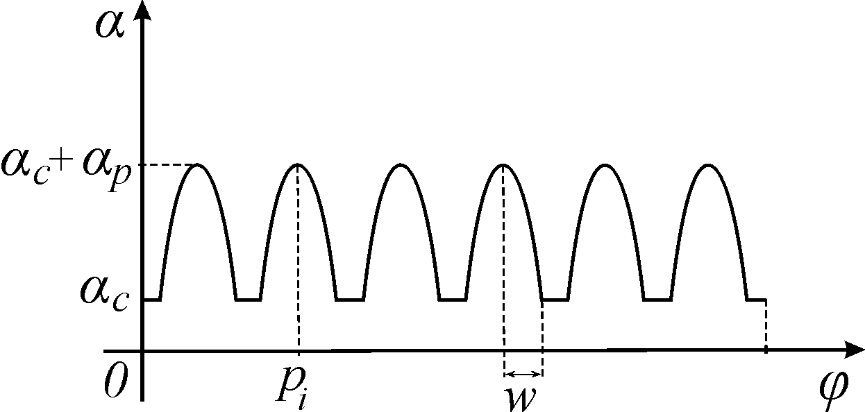
Figure 2:

In one cooling section the same type spray nozzles are installed. They give an identical water-air spray. Hence the CHTC is the same parabola shifted along the abscissa axis (fig. 2).

All sites under spray nozzles can be reduced to the coordinate origin so that the peak of each parabola should be over the coordinate origin. Hence, it is necessary to define only two parameters - $\alpha_{p}$ and $\alpha_{c}$. So, $\alpha(\varphi)$ is given by

$$\alpha(\varphi)=\alpha_{c}-\frac{\alpha_{p}}{w^{2}}\varphi^{2}+\alpha_{p}.$$

Consider the parts of the section, on which $\alpha(\varphi)=\alpha_{c}=const$. Let $K$ be the ensemble of points $\varphi_{i}$, in which CHTC is equal to constant. Let $B$ be the ensemble of other points.

The finite-difference approximation of boundary condition (11) is

$$\lambda_{i,0}\frac{T_{i,2}-4T_{i,1}+3T_{i,0}}{2q}=\alpha_{c}(T_{I_{1}}-T_{i,0})+C_{I_{1}}(T_{I_{1}}^{4}-T_{i,0}^{4}),$$

where $q$ – step of finite-difference grid by radius $r_{1}$ [3].

It follows that the discrepancy of heat flows on the boundary is:

$$\Delta=\lambda_{i,0}\frac{T_{i,2}-4T_{i,1}+3T_{i,0}}{2q}-C_{I_{1}}\left({T_{I_{1}}^{4}-T_{i,0}^{4}}\right)-\alpha_{c}\left({T_{I_{1}}-T_{i,0}}\right).$$

Let us denote

$$P_{i}=\lambda_{i,0}\frac{T_{i,2}-4T_{i,1}+3T_{i,0}}{2q}-C_{I_{1}}\left({T_{I_{1}}^{4}-T_{i,0}^{4}}\right),\quad Q_{i}=T_{I_{1}}-T_{i,0}.$$

Then we find a value $\alpha_{c}$, such that the sum of squares of discrepancies is minimum, i.e. the follow condition is satisfied

$$S=\sum\limits_{i}{(P_{i}-\alpha_{c}Q_{i})^{2}}\to\min,\quad\quad\forall i:\varphi_{i}\in K.$$

A necessary condition of the extremum existence of the function $S(\alpha_{c})$ is:

$$\frac{\partial S}{\partial\alpha_{c}}=-2\sum\limits_{i}{Q_{i}}(P_{i}-\alpha_{c}Q_{i})=0.$$

It follows that

$$\alpha_{c}=\frac{\sum\limits_{i}{Q_{i}P_{i}}}{\sum\limits_{i}{Q_{i}^{2}}}.$$

To the each point $\varphi_{i}$ from we will put in conformity a point $y_{i}$ on the segment $\left[{-w,\,\,w}\right]$ such that $\left|{y_{i}}\right|$ is equal to the distance from the corresponding $\varphi_{i}$ to the coordinate of the nearest spray nozzle. From (18) and (19) we gain a discrepancy

$$\Delta=\lambda_{i,0}\frac{T_{i,2}-4T_{i,1}+3T_{i,0}}{2q}-C_{I_{1}}\left({T_{I_{1}}^{4}-T_{i,0}^{4}}\right)-\left({\alpha_{c}-\frac{\alpha_{p}}{w^{2}}y_{i}^{2}+\alpha_{p}}\right)\left({T_{I_{1}}-T_{i,0}}\right).$$

Then we can find a value $\alpha_{p}$, such that the sum

$$S=\sum\limits_{i}{(P_{i}-(\alpha_{c}-\frac{\alpha_{p}}{w^{2}}y_{i}^{2}+\alpha_{p})\cdot Q_{i})^{2}}\to\min.$$

From the following necessary condition of extremum existence

$$\frac{\partial S}{\partial\alpha_{p}}=2\sum\limits_{i}{\left({P_{i}-\left({\alpha_{c}-\alpha_{p}\left({\frac{y_{i}^{2}}{w^{2}}-1}\right)}\right)P_{i}}\right)\left({Q_{i}\left({\frac{y_{i}^{2}}{w^{2}}-1}\right)}\right)}=0$$

we obtain $\alpha_{p}$

$${\displaystyle\ \alpha_{p}=\frac{{\displaystyle\ \alpha_{c}\sum\limits_{i}{Q_{i}^{2}\left({\frac{y_{i}^{2}}{w^{2}}}-1\right)}}-{\displaystyle\ \sum\limits_{i}{P_{i}Q_{i}\left({\frac{y_{i}^{2}}{w^{2}}-1}\right)}}}{{\displaystyle\ \sum\limits_{i}{Q_{i}^{2}\left({\frac{y_{i}^{2}}{w^{2}}-1}\right)^{2}}}}.}$$

On fig. 3 comparative results of calculations (1 – by the method of direct reversion, 2 – by the least squares method) are presented. For steel grade st40, width of a slab is 1m, l = 0,1m and v = 1(m/minute). The decision obtained by the method of direct reversion is unstable and unsuitable for practical use. The second curve represents a spline approximation, which is gained as a result of the decision of a problem of identification by the least squares method.

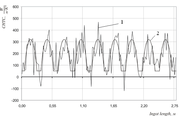
Figure 3:

Thus, we fined the spline approximation of the CHTC, which is distributed on the surface of the moving ingot. This approximation gives the minimum of mean-square deviation between measured surface temperature and calculated one according to the model as the result of solving of the direct problem. The CHTC for other sections of the secondary cooling zone is analogously defined. It should be noted that an advantage of the offered method is that the estimation error of the least squares method is negligibly small by relatively small number of abnormal measurements. It is very important in case of temperature measurement of a partially oxide scaled ingot surface.

4 Operative adjustment of convective heat transfer coefficient (CHTC)

CHTC obtained by initial adjustment varies under changes of various parameters of process (for example, ambient temperatures). Therefore, it is necessary to provide its operative adaptation during work CCM. The fine-tuning of parameters should be carried out in real time. But during usual work of CCM the information on a thermal condition of an ingot is limited to temperature indications in small number of points of the surface of an ingot. Such algorithms can be based on the stochastic approximation method [4].

The temperature on the ingot surface is measured in every equal small time intervals. Let us denote the measuring temperature data $T_{j}^{*}$. The computer models the casting process using the presented mathematical model. The under model calculated temperature in the corresponding point we denote by $T_{j}$. It is necessary to correct the model parameters using information about deviations between measured and calculated temperature data to reduce these deviations to minimum. The difficulty of the decision of the given problem is that temperature measurements are deformed by a random telemetry error.

Operative fine-tuning consists in refinement of the constant value $\alpha_{c}$, which defines the distribution of the convective heat transfer coefficient obtained by the solving of the problem of the initial adjustment of parameters.

For using the algorithm of stochastic approximation it is necessary, that the random error of temperature indications would have the zero average and the finite variance.

The algorithm of parameter adjustment is

$$\alpha_{j+1}=\alpha_{j}-k_{j}(T_{j}^{\ast}-T_{j}),$$

where $\alpha_{j}$ – $j$-th approximate value of $\alpha_{c}$, $k_{j}$ – special sequence of numbers, which satisfies to the following conditions:

$$\mathop{\lim}\limits_{j\to\infty}k_{j}=0,\quad\sum\limits_{j=1}^{\infty}{k_{j}=\infty},\quad\sum\limits_{j=1}^{\infty}{(k_{j})^{2}<\infty}.$$

For example the following elementary sequence satisfies to such conditions

$$k_{j}=\frac{a}{b+j},$$

where $a,\;b\;\in R$, $a>0$. Selecting numbers $a$ and $b$, and also other sequences satisfying to the conditions (21), it is possible to change speed of convergence of algorithm. In [3], for example, it is recommended to keep $k_{j}$ as constant while the sign of discrepancy $T_{j}^{\ast}-T_{j}$ not vary, and change then $k_{j}$ so that to satisfy to above mentioned restrictions.

Truncation condition of the parameter fine tuning algorithm work is occurrence of m last received approximations $\alpha_{n+1},\alpha_{n+2},,\alpha_{n+m}$ in a vicinity of $\alpha_{n}$ serves:

$$|\alpha_{n}-\alpha_{n+i}|<\varepsilon,\quad\forall i=1,,m.$$

If the condition is executed, assume $\alpha_{c}$ is equal $\alpha_{n}$. For check we use values CHTC which have been picked up experimentally at the decision of a direct problem of modeling of thermal field CCM [1].

5 Examples of realization of the stochastic approximation method

Numerical modeling allows establishing the basic features of trajectories of parameter fine-tuning process. On fig. 4 trajectories of parameter fine-tuning, characterizing a deviation of the distributed parameter from true value, for the algorithm using sequence

$$k_{j}=\frac{a}{j},\quad j=1,2,3,...$$

are presented at various values of factor $a$. When $a<1$ very slow convergence is observed. In this case the time of parameter tuning is inadmissible big.

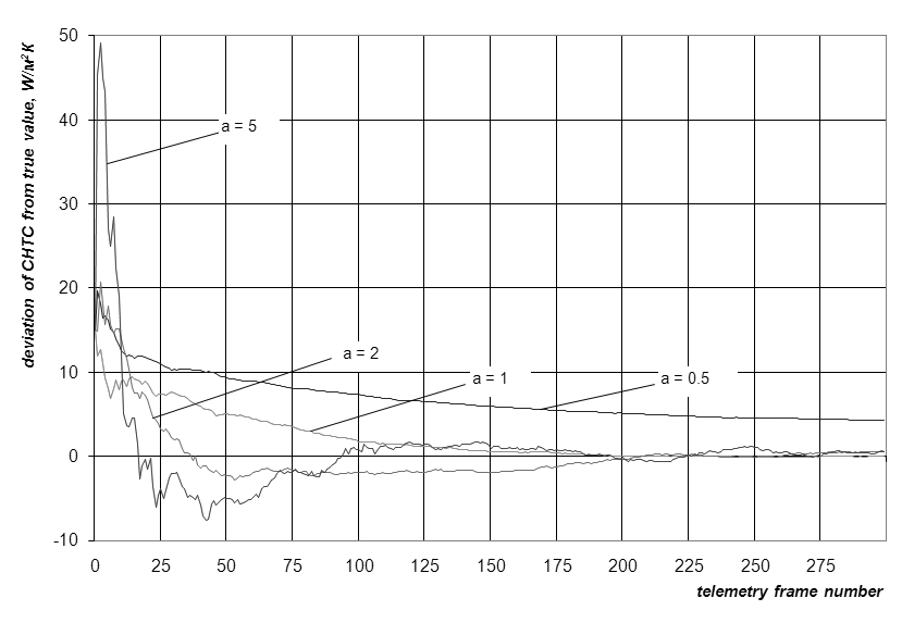
Figure 4:

If to choose $a=1$ the value of the parameter is in enough small vicinity of true value approximately after 200th iteration. At $a=2$ the trajectory of parameter fine-tuning reflects oscillations with damped amplitude and frequency and not later than for 200 iterations the parameter is adjusted. At increase $a>2$ the amplitude of oscillations grows. In this case also oscillations with damped amplitude and frequency are observed, but for fine-tuning it is required considerably more iterations.

From here we conclude, that for the chosen sequence the best values of the factor $a$ is a number from interval $1\leq a\leq 2$.

We investigate now influence of value $b$ on speed of the algorithm’s convergence. On fig. 5 trajectories of parameter fine-tuning are shown for various values $b$. Values $b$ less than zero lead to that fine-tuning go in a ”wrong” direction while the denominator is negative and at $i=-b$ the denominator is equal to zero. Increase $b$ leads to decrease of a velocity of convergence of algorithm. The same results have been obtained for sequences, which will be described further. Therefore further parameter $b$ everywhere will be chosen equal to zero.

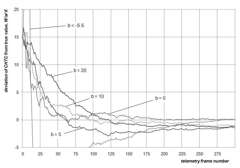
Figure 5:

The following sequence also satisfies to conditions (21)

$$k_{j}=\frac{a}{n_{j}},\quad n_{j+1}=\left\{{\begin{array}[]{l}n_{j},\quad\quad(T_{j}^{\ast}-T_{j})(T_{j+1}^{\ast}-T_{j+1})>0\\ j+1,\;\quad(T_{j}^{\ast}-T_{j})(T_{j+1}^{\ast}-T_{j+1})\leq 0\\ \end{array}}\right..$$

Results of this algorithm work are presented on fig. 6. In this case factor $a$ needs to be chosen within $1\leq a\leq 3$. Values out of this range give smaller speed of algorithm convergence.

Consider another sequence, which also satisfies to conditions (21)

$$k_{j}=\frac{a}{n_{j}},\quad n_{j+1}=\left\{{\begin{array}[]{l}n_{j},\quad\;\quad(T_{j}^{\ast}-T_{j})(T_{j+1}^{\ast}-T_{j+1})>0\\ n_{j}+1,\quad\;(T_{j}^{\ast}-T_{j})(T_{j+1}^{\ast}-T_{j+1})\leq 0\\ \end{array}}\right..$$

It has slower convergence than the previous two sequences. Results of calculations with use of this sequence are presented on fig. 7. Factor $a$ can be chosen within $0.5\leq a\leq 2$. And, if $1.2\leq a\leq 1.5$, than obtained approximations differ from the true value no more than on 6 % after 20 iterations already.

Figure 6:

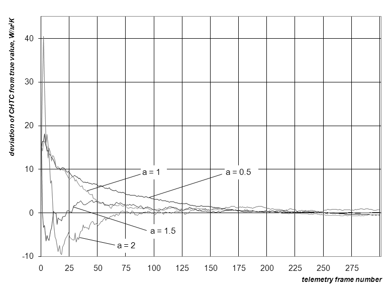
Figure 7:

In the conclusion also it is necessary to notice, that the advantage of stochastic approximation algorithm is its successful work for enough wide interval of initial values of the distributed parameter.

References

[1]
[2]Tkachenko V.N., Ivanova A.A. Modeling and Analysis of
Temperature Field of Ingot of Curvilinear Continuous Casting
Machine. – Electronic Modeling - 2008. Vol.30, 3. p.87-103.
(in russian)
[3]
[4]Tkachenko V.N. Heat processes modeling in automatic system of
information handling. //Visnyk Donetskogo Natsionalnogo
Universytetu, Ser.A, ’Pryrodnychi nauky’, 2002, No 2, p.379 - 383.
(in russian)
[5]
[6]Marchuk G.I. Methods of computational mathematics. – Moskow:
Nauka, 1980, 535 c. (in russian)
[7]
[8]Andrew P. Sage, James L. Melsa System Identification. –
System Identification. Academic Press, 1971, New York and London.