Relationship between quantum walks and relativistic quantum mechanics

Abstract

Quantum walk models have been used as an algorithmic tool for quantum computation and to describe various physical processes. This paper revisits the relationship between relativistic quantum mechanics and the quantum walks. We show the similarities of the mathematical structure of the decoupled and coupled form of the discrete-time quantum walk to that of the Klein-Gordon and Dirac equations, respectively. In the latter case, the coin emerges as an analog of the spinor degree of freedom. Discrete-time quantum walk as a coupled form of the continuous-time quantum walk is also shown by transforming the decoupled form of the discrete-time quantum walk to the Schrödinger form. By showing the coin to be a means to make the walk reversible, and that the Dirac-like structure is a consequence of the coin use, our work suggests that the relativistic causal structure is a consequence of conservation of information. However, decoherence (modelled by projective measurements on position space) generates entropy that increases with time, making the walk irreversible and thereby producing an arrow of time. Lieb-Robinson bound is used to highlight the causal structure of the quantum walk to put in perspective the relativistic structure of quantum walk, the maximum speed the walk propagation and the earlier findings related to the finite spread of the walk probability distribution. We also present a two-dimensional quantum walk model on a two state system to which the study can be extended.

I Introduction

Quantum walks are the quantum analog of the classical random walks Ria58 ; FH65 ; ADZ93 developed using the aspects of quantum mechanics such as interference and superposition. Like their classical counterpart, quantum walks are also widely studied in two forms: continuous-time quantum walk FG98 and discrete-time quantum walk ADZ93 ; DM96 ; ABN01 ; NV01 . In the continuous-time quantum walk, one can directly define the walk on the position Hilbert space $\mathcal{H}_{p}$, whereas in the discrete-time quantum walk, it is necessary to introduce a quantum coin operation, an additional coin Hilbert space $\mathcal{H}_{c}$ to define the direction in which the particle has to evolve in position space. The results from the continuous-time quantum walk and the discrete-time quantum walk are often similar, but because of the coin degree of freedom, the discrete-time variant has been shown to be more powerful than the other in some contexts AKR05 .

Quantum walks have emerged as a powerful tool in the development of quantum algorithms Amb03 ; CCD03 ; SKB03 . Furthermore, it has been used to demonstrate the coherent quantum control over atoms, quantum phase transition CL08 , to explain phenomena such as breakdown of an electric-field driven system OKA05 and direct experimental evidence for wavelike energy transfer within photosynthetic systems ECR07 ; MRL08 . Experimental implementation of the quantum walk has been reported with samples in nuclear magnetic resonance system DLX03 ; RLB05 ; in the continuous tunneling of light fields through waveguide lattices PLP08 ; in the phase space of trapped ions SMS09 ; ZKG10 based on the scheme proposed by TM02 ; with single optically trapped atoms KFC09 ; and with single photon BFL10 . Various other schemes have been proposed for its physical realization in different physical systems RKB02 ; EMB05 ; Cha06 ; MBD06 .

The relationship between the idea of quantum walk and relativistic quantum mechanics goes back to the discrete version of the one-dimensional Dirac equation propagator considered by Feynman and Hibbs FH65 . Later, similarities of the relativistic wave equations and unitary cellular and quantum lattice gas automata were observed by Bialynicki-Birula Bia94 and Meyer DM96 . Recently, that is, after the extensive studies of the one-dimensional discrete-time quantum walk, the relationship between quantum walk models and relativistic quantum mechanics has become a topic of interest KFK05 ; Str06 ; BES07 ; Str07 ; Kur08 ; SK10 . In reference KFK05 , the one-dimensional quantum walk is mapped to the three-dimensional Weyl equation. In different continuum limits, the discrete-time quantum walk was shown to be equivalent to the one-dimensional Dirac equation and the continuous-time quantum walk, respectively Str06 ; Str07 . In reference BES07 , the evolved probability density for the Dirac particle was obtained from the asymptotic form of the probability distribution of the quantum walk. The effects similar to the relativistic effects, namely, Zitterbewegung and Klein’s paradox, were shown to be present in the discrete-time quantum walk Kur08 , and in reference SK10 , the Dirac equation with ultraviolet cutoff is shown to provide a discrete-time quantum walk in three dimensions on a four-component qubit SK10 .

The main focus of this article is to present in detail the dynamics of the discrete-time quantum walk and the similarity of its mathematical structure to that of the relativistic quantum mechanical evolution. We compare the similarities of the mathematical structures of the decoupled and coupled forms of the discrete-time quantum walk to those of the relativistic free spin-$0$ particles Klein-Gordon and free spin-$1/2$ particles Dirac equations, respectively. In the latter case, the coin emerges as an analog of the spinor degree of freedom. By showing the coin to be a means to make the walk reversible, and that the Dirac-like structure is a consequence of the coin use, our work suggests that the relativistic causal structure is a consequence of conservation of information. We also discuss the origin of time asymmetry in the projective measurement on position space producing the arrow of time and making the walk irreversible. The arrow of time in the quantum walk also been discussed recently SCS10 . Discrete-time quantum walk as a coupled form of the continuous-time quantum walk is also shown by transforming the decoupled form of the discrete-time quantum walk to the Schrödinger form. The probability distribution for discrete-time quantum walk evolution spreads in time, but this spreading is controlled by the coin operation used during the evolution. The presence of a speed limit in a discrete-time quantum walk dynamics is, in fact, an instance of a much more general phenomenon know as the Lieb-Robinson bound. Two-dimensional quantum walk using a two-state particle is presented, to which the study can be extended.

In Sec. II, we will first review the continuous-time quantum walk which follows the Schrödinger form of evolution. In Sec. III, we will review the discrete-time quantum walk model : In Sec. III.1, the dynamic structure of the discrete-time quantum walk is discussed, followed by the consequence of the projective measurement on the system, that is, the arrow of time, in Sec. III.2. In Sec. IV, we will study the mathematical structure of the one-dimensional discrete-time quantum walk: its decoupled form and similarities to the free spin-$0$ relativistic form, that is, the Klein-Gordon form (Sec. IV.1) and Schrödinger form (Sec. IV.2), and its coupled form and similarities to the Dirac form (Sec. IV.3). In Sec. V, we present the Lieb-Robinson bound-like effect in quantum walk evolution. In Sec. VI, a two-dimensional discrete-time quantum walk model using a two-state particle, to which the study can be extended, is presented before concluding in Sec. VII.

II Continuous-time quantum walk

To define the continuous-time quantum walk, it is easier first to define the continuous-time classical random walk and quantize it by introducing quantum amplitudes in place of classical probabilities.

The continuous-time classical random walk takes place entirely in the position space. To illustrate, let us define a continuous-time classical random walk on the position space $\mathcal{H}_{p}$ spanned by a vertex set $V$ of a graph $G$ with edge set $E$, $G=(V,E)$. A step of the random walk can be described by an adjacency matrix $A$ which transforms the probability distribution over $V$; that is,

$$A_{j,k}=\begin{cases}1&~{}~{}(j,k)\in E,\\ 0&~{}~{}(j,k)\notin E,\end{cases}$$ (1)

for every pair $j,k\in V$. The other important matrix associated with the graph $G$ is the generator matrix ${\bf H}$ given by

$${\bf H}_{j,k}=\begin{cases}d_{j}\gamma&~{}~{}j=k\\ -\gamma&~{}~{}(j,k)\in E\\ 0&~{}~{}{\rm otherwise}\end{cases},$$ (2)

where $d_{j}$ is the degree of the vertex $j$ and $\gamma$ is the probability of transition between neighboring nodes per unit time.

If $p_{j}(t)$ denotes the probability of being at vertex $j$ at time $t$, then the transition on graph $G$ is defined as the solution of the differential equation

$$\frac{d}{dt}p_{j}(t)=-\sum_{k\in V}{\bf H}_{j,k}p_{k}(t).$$ (3)

The solution of the differential equation is given by

$$p(t)=e^{-{\bf H}t}p(0).$$ (4)

By replacing the probabilities $p_{j}$ by quantum amplitudes $a_{j}(t)=\langle j|\psi(t)\rangle$ where $|j\rangle$ is spanned by the orthogonal basis of the position Hilbert space $\mathcal{H}_{p}$ and introducing a factor of $i$ we obtain

$$i\frac{d}{dt}a_{j}(t)=\sum_{k\in V}{\bf H}_{j,k}a_{k}(t).$$ (5)

We can see that Eq. (5) is the Schrödinger equation

$$i\frac{d}{dt}|\psi\rangle={\bf H}|\psi\rangle.$$ (6)

Since the generator matrix is an Hermitian operator, the normalization is preserved during the dynamics. The solution of the differential equation can be written in the form

$$|\psi(t)\rangle=e^{-i{\bf H}t}|\psi(0)\rangle.$$ (7)

Therefore the continuous-time quantum walk is of the form of the Schrödinger equation, a nonrelativistic quantum evolution.

To implement the continuous-time quantum walk on a line, the position Hilbert space $\mathcal{H}_{p}$ can be written as a state spanned by the basis states $|\psi_{j}\rangle$, where $j\in\mathbb{Z}$. The Hamiltonian ${\bf H}$ is defined such that

$${\bf H}|\psi_{j}\rangle=-\gamma|\psi_{j-1}\rangle+2\gamma|\psi_{j}\rangle-\gamma|\psi_{j+1}\rangle$$ (8)

and evolves the system through time $t$ via the transformation

$$U(t)=\exp(-i{\bf H}t).$$ (9)

The Hamiltonian ${\bf H}$ of the process acts as the generator matrix which will transform the probability amplitude at the rate of $\gamma$ to the neighboring sites, where $\gamma$ is a time-independent constant.

III One-dimensional discrete-time quantum walk

We will first define the structure of the one-dimensional discrete-time classical random walk. The discrete-time classical random walk takes place on the position Hilbert space $\mathcal{H}_{p}$ with instruction from the coin operation. A coin flip defines the direction in which the particle moves, and a subsequent position shift operation moves the particle in position space. For a walk on a line, a two-sided coin with a head and a tail defines the movements to the left and right side, respectively.

The one-dimensional discrete-time quantum walk also has a very similar structure to that of its classical counterpart. The coin flip is replaced by the quantum coin operation which defines the superposition of direction in which the amplitude of the particle evolves simultaneously. The quantum coin operation followed by the unitary shift operation is iterated without resorting to intermediate measurement to implement a large number of steps. During the walk on a line, interference between the left- and the right- propagating amplitude results in the quadratic growth of variance with the number of steps.

The discrete-time quantum walk on a line is defined on a Hilbert space

$$\mathcal{H}=\mathcal{H}_{c}\otimes\mathcal{H}_{p},$$ (10)

where $\mathcal{H}_{c}$ is the coin Hilbert space and $\mathcal{H}_{p}$ is the position Hilbert space. For a discrete-time quantum walk in one dimension, $\mathcal{H}_{c}$ is spanned by the basis state (internal state) of the particle $|0\rangle$ and $|1\rangle$, and $\mathcal{H}_{p}$ is spanned by the basis state of the position $|\psi_{j}\rangle$, where $j\in\mathbb{Z}$. To implement the discrete-time quantum walk on a particle at origin in state

$$|\Psi_{in}\rangle=\left(\cos(\delta)|0\rangle+e^{i\eta}\sin(\delta)|1\rangle\right)\otimes|\psi_{0}\rangle,$$ (11)

the quantum coin toss operation $B\in U(2)$, which in general can be written as

$$B_{\zeta,\alpha,\beta,\gamma}=e^{i\zeta}e^{i\alpha\sigma_{x}}e^{i\beta\sigma_{y}}e^{i\gamma\sigma_{z}},$$ (12)

is applied, where $\sigma_{x},\sigma_{y}$, and $\sigma_{z}$ are the Pauli spin operators. Parameters of the coin operations $\zeta,\alpha,\beta,\gamma$ can be varied to get different superposition states of the particle; that is, quantum coin operation $B_{\zeta,\alpha,\beta,\gamma}$ is used to evolve the particle to superposition of its basis states such that it can serve as an instruction to simultaneously evolve the particle to the $left$ and $right$ of its initial position. The quantum coin operation is followed by the conditional unitary shift operation $S$ given by

$$S = e^{-i(|0\rangle\langle 0|-|1\rangle\langle 1|)\otimes\hat{Pl}}=\left(|0\rangle\langle 0|\otimes e^{-i\hat{P}l}\right)+\left(|1\rangle\langle 1|\otimes e^{i\hat{P}l}\right),$$ (13)

where $\hat{P}$ is the momentum operator, $l$ is the step length, and $|0\rangle$ and $|1\rangle$ are the basis states of the particle. Therefore the operator $S$, which delocalizes the wave packet in different basis states $|0\rangle$ and $|1\rangle$ over the position $(j-1)$ and $(j+1)$ when step length $l=1$, can also be written as

$$S=|0\rangle\langle 0|\otimes\sum_{j\in\mathbb{Z}}|\psi_{j-1}\rangle\langle\psi_{j}|+|1\rangle\langle 1|\otimes\sum_{j\in\mathbb{Z}}|\psi_{j+1}\rangle\langle\psi_{j}|.$$ (14)

The states in the new position are again evolved into the superposition of its basis state and the process of quantum coin toss operation $B_{\zeta,\alpha,\beta,\gamma}$ followed by the conditional unitary shift operation $S$,

$$W_{\zeta,\alpha,\beta,\gamma}=S(B_{\zeta,\alpha,\beta,\gamma}\otimes{\mathbbm{1}})$$ (15)

is iterated without resorting to intermediate measurement, to realize a large number of steps of the discrete-time quantum walk. The four variable parameters of the quantum coin, $\zeta,\alpha,\beta$, and $\gamma$ in Eq. (12) can be varied to change and control the probability amplitude distribution in the position space.

The most widely studied form of the discrete-time quantum walk is the Hadamard walk, using the Hadamard operation $H=\frac{1}{\sqrt{2}}\left(\begin{array}[]{clcr}1&&~{}1\\ 1&&-1\end{array}\right)$ as a quantum coin operation, and the role of the coin operation and initial state to control the probability amplitude distribution has been discussed in earlier studies ABN01 ; BCG04 . It has been demonstrated that a three-parameter $SU(2)$ quantum coin operation,

$$B_{\xi,\theta,\zeta}\equiv\left(\begin{array}[]{clcr}\mbox{~{}}e^{i\xi}\cos(\theta)&&e^{i\zeta}\sin(\theta)\\ -e^{-i\zeta}\sin(\theta)&&e^{-i\xi}\cos(\theta)\end{array}\right)$$ (16)

is sufficient to describe the most general form of the discrete-time quantum walk CSL08 .

III.1 Dynamic structure of discrete-time quantum walk

The standard symmetric discrete-time classical random walk leads to

$$p(j,t+1)=\frac{1}{2}\left[p(j-1,t)+p(j+1,t)\right],$$ (17)

where $p(j,t)$ denotes the probability of finding the particle at position $j$ at discrete time $t$. This equation expresses the fact that all the probability at a given site is transmitted out at each time step, so that the probability available at it in the next time step is that received in equal measure from its immediate neighbors. Subtracting $p(j,t)$ from both sides of Eq. (17) leads to the difference equation which corresponds to differential equation

$$\frac{\partial}{\partial t}p(j,t)=\frac{\partial^{2}}{\partial^{2}j}p(j,t),$$ (18)

which is the standard classical diffusion equation. The preceding equation is irreversible because the coin is effectively thrown away after each toss. It is also nonrelativistic in the sense that it is not symmetric in time and space and leads to a dispersion relation that is nonrelativistic Str07 . On the contrary, in the discrete-time quantum walk, the information of the state of the quantum coin in the previous step is retained and carried over to the next step. This makes the quantum walk reversible.

To illustrate this, we consider the wave function describing the position of a particle and analyze how it evolves with time $t$. Let $t$ be the time required to implement $t$ steps of the quantum walk. The two-component vector of amplitudes of the particle, being at position $j$, at time $t$, with left-moving ($L$) and right-moving ($R$) components, is given by

$$\Psi(j,t)=\left(\begin{array}[]{cl}\Psi_{L}(j,t)\\ \Psi_{R}(j,t)\end{array}\right).$$ (21)

A single-variable parameter quantum coin operation of the form

$$B_{0,\theta,-\frac{\pi}{2}}=\left(\begin{array}[]{ccc}\mbox{~{}~{}~{}}\cos(\theta)&{}\hfil&-i\sin(\theta)\\ -i\sin(\theta)&{}\hfil&\mbox{~{}~{}~{}}\cos(\theta)\end{array}\right)$$ (22)

is used to drive the dynamics for $\Psi(j,t)$. The coin parameters $(0,\theta,-\frac{\pi}{2})$ have been used here to achieve a symmetrical form of the coin operation on the particle. The quantum coin operation is followed by the conditional shift operator $S$; that is, $S(B_{0,\theta,-\frac{\pi}{2}}\otimes{\mathbbm{1}})$ in terms of left-moving ($L$) and right-moving ($R$) components at a given position $j$ and time $t+1$ is given by

$$\left(\begin{array}[]{cl}\Psi_{L}(j,t+1)\\ \Psi_{R}(j,t+1)\end{array}\right)=\left(\begin{array}[]{ccc}\mbox{~{}~{}~{}}\cos(\theta)a&{}\hfil&-i\sin(\theta)a^{\dagger}\\ -i\sin(\theta)a^{\dagger}&{}\hfil&\mbox{~{}~{}~{}}\cos(\theta)a\end{array}\right)\left(\begin{array}[]{cl}\Psi_{L}(j,t)\\ \Psi_{R}(j,t)\end{array}\right),$$ (29)

where action of operator $a$ and $a^{\dagger}$ on $\Psi(j,t)$ is given by

$$a\Psi(j,t)=\Psi(j+1,t),$$ (30a)

$$a^{\dagger}\Psi(j,t)=\Psi(j-1,t).$$ (30b)

Therefore,

$$\Psi_{L}(j,t+1) = \cos(\theta)\Psi_{L}(j+1,t)-i\sin(\theta)\Psi_{R}(j-1,t),$$ (31a)

$$\Psi_{R}(j,t+1) = \cos(\theta)\Psi_{R}(j-1,t)-i\sin(\theta)\Psi_{L}(j+1,t).$$ (31b)

We thus find that the coin degree of freedom is carried over during the dynamics of the discrete-time quantum walk, making it reversible.

III.2 Projective measurement, irreversibility and arrow of time

From Eqs. (31a) and (31b), we noted that the coin degree of freedom is carried over during the dynamics of the discrete-time quantum walk, making walk reversible; that is, the information is stored during the evolution so that it can be used to reverse the dynamics. However, upon projective measurement on the position space, the information of the coin is lost, making the walk irreversible. The projective measurement produces the arrow of time since its description is time asymmetric. Therefore an increase in measurement entropy of the system can be seen as an arrow of time.

This projective measurement of position happening with step time 1 can be understood as an interaction with the environment. Quantum diffusion via walk by itself does not generate entropy (being unitary); rather interaction with the environment generates entropy that increases with time. Figure (1) depicts the increase in measurement entropy with the increase in time. Measurement entropy is calculated by considering the Shannon entropy of the particle position probability distribution $p_{j}$ obtained by tracing over the coin basis:

$$H(j)=-\sum_{j=-t}^{+t}p_{j}\log p_{j},$$ (32)

where $j$ is spanned over the position space at time $t$.

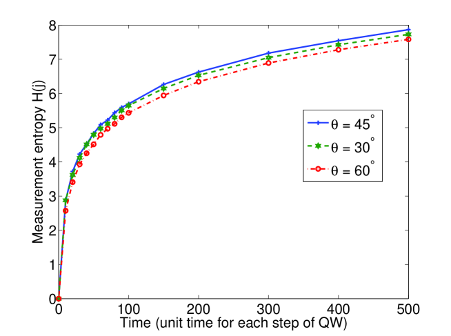
Figure 1: (Color online) Increase in measurement entropy ($H(j)$) with time when unit time is required to implement each step of quantum walk. Increase in entropy indicate the arrow of time. Measurement entropy was calculated for quantum walk for up to 500 units in time using $B_{0,45^{\circ},0}$, $B_{0,30^{\circ},0}$ and $B_{0,60^{\circ},0}$ as quantum coin operations.

This time dependence can be understood as follows: the position measurement generates entropy, which in each instance of measurement is translated into a classical record. That larger record of information is needed if the system is measured at a later rather than an earlier time, to reconstruct the original state. This can be construed as giving the direction of time. Following reference Mac09 , we may say that if the record for some process actually diminished along a direction of a time, there would be no objective knowledge of the process (here the walk) having happened.

IV Relativistic features in discrete-time quantum walk

IV.1 Decoupled discrete-time quantum walk equation in Klein-Gordon form

The discrete-time quantum walk can be written in a free spin-$0$ particles relativistic form, that is, in the Klein-Gordon form, by decoupling the components $\Psi_{L}$ and $\Psi_{R}$ in Eqs. (31a) and (31b) (Appendix A):

$$\Psi_{R}(j,t+1)+\Psi_{R}(j,t-1)=\cos(\theta)[\Psi_{R}(j+1,t)+\Psi_{R}(j-1,t)],$$ (33a)

$$\Psi_{L}(j,t+1)+\Psi_{L}(j,t-1)=\cos(\theta)[\Psi_{L}(j+1,t)+\Psi_{L}(j-1,t)].$$ (33b)

Subtracting $2\Psi_{R}(j,t)+2\cos(\theta)\Psi_{R}(j,t)$ from both sides in Eq. (33a), we obtain a difference equation which corresponds to differential equation

$$\left[\cos(\theta)\frac{\partial^{2}}{\partial j^{2}}-\frac{\partial^{2}}{\partial t^{2}}\right]\Psi_{R}(j,t)=2(1-\cos(\theta))\Psi_{R}(j,t),$$ (34)

by setting the time step and spatial step to 1; see Appendix B for intermediate steps. A similar expression can be obtained for $\Psi_{L}(j,t)$. This shows that each component follows a Klein-Gordon equation of the form

$$\left(\nabla^{2}-\frac{1}{c^{2}}\frac{\partial^{2}}{\partial t^{2}}\right)\phi-\mu^{2}\phi=0,$$ (35)

showing essentially the free spin-0 particles relativistic character of each component of the discrete-time quantum walk.

We obtain from Eq. (34) the equivalent of light speed $c$ and mass $m$ of each component $\Psi_{R}$ and $\Psi_{L}$ of the discrete-time quantum walk dynamics :

$$c \equiv \sqrt{\cos(\theta)},$$ (36)

$$\mu=\frac{mc}{\hbar} \equiv \sqrt{2[\sec(\theta)-1]}.$$ (37)

Considering $\hbar=1$, we can write

$$m \equiv \sqrt{\frac{2[\sec(\theta)-1]}{\cos(\theta)}}.$$ (38)

Note that the maximum velocity is given by $c=1$, corresponding to $\theta=0$ and $m=0$, which is in agreement with the relativistic requirement that the rest mass of light vanishes. This is also in agreement with the quantum walk dynamics that $\theta=0$ corresponds to state $|0\rangle$ and $|1\rangle$ moving away from each other without any interference, resulting in maximum variance CSL08 . The relativistic nature of the quantum walk thus arises as a natural consequence of employing the coin. Since, as noted earlier, the coin makes the walk reversible, we have the interesting scenario that the relativistic causal structure is fundamentally a consequence of conservation of information. This is in accordance with some recent works that have studied possible information theoretical bases for the mathematical structure of quantum mechanics CZ09 ; CBH03 ; SBG01 ; Sri06 .

IV.2 Decoupled discrete-time quantum walk equation in Schrödinger form

The Klein-Gordon equation can be transformed into the Schrödinger formulation Gre . Transforming the discrete-time equation, Eq. (34) - which is of the second order in the time coordinate - into a system of two coupled differential equations that are of first order in time is achieved by the ansatz

$$\Psi_{R}=\varphi_{R}+\chi_{R}~{}~{}~{}~{}~{}~{},~{}~{}~{}~{}~{}i\hbar\frac{\partial\Psi_{R}}{\partial t}=\sqrt{2[1-\cos(\theta)]}~{}(\varphi_{R}-\chi_{R}),$$ (39)

in which $\Psi_{R}$ and its time derivative $\partial\Psi_{R}/\partial t$ are expressed as components of two functions $\varphi_{R}$ and $\chi_{R}$.

Now we can show that the two coupled differential equations,

$$i\hbar\frac{\partial\varphi_{R}}{\partial t}=-\frac{\hbar^{2}}{2\sqrt{\frac{2[\sec(\theta)-1]}{\cos(\theta)}}}~{}\Delta(\varphi_{R}+\chi_{R})+\sqrt{2[1-\cos(\theta)]}~{}\varphi_{R},$$ (40a)

$$i\hbar\frac{\partial\chi_{R}}{\partial t}=\frac{\hbar^{2}}{2\sqrt{\frac{2[\sec(\theta)-1]}{\cos(\theta)}}}~{}\Delta(\varphi_{R}+\chi_{R})-\sqrt{2[1-\cos(\theta)]}~{}\chi_{R},$$ (40b)

are equivalent to the discrete-time quantum walk equation in relativistic form [Eq. (34)] (Appendix C).

The coupled Eqs. (40a) and (40b) may be combined to form one equation by introducing the column vector

$$\Psi_{R}=\left(\begin{array}[]{c}\varphi_{R}\\ \chi_{R}\end{array}\right)$$ (41)

and making use of the four $2\times 2$ matrices

$$\sigma_{1}=\left(\begin{array}[]{ccc}0&&1\\ 1&&0\end{array}\right),~{}~{}~{}~{}~{}\sigma_{2}=\left(\begin{array}[]{ccc}0&&-i\\ i&&0\end{array}\right),~{}~{}~{}~{}~{}~{}~{}~{}~{}\sigma_{3}=\left(\begin{array}[]{ccc}1&&0\\ 0&&-1\end{array}\right),~{}~{}~{}~{}\mathbbm{1}=\left(\begin{array}[]{ccc}1&&0\\ 0&&1\end{array}\right),$$ (42)

which satisfy the algebraic relations

$$\sigma_{k}^{2}=\mathbbm{1}~{}~{},~{}~{}~{}~{}\sigma_{k}\sigma_{l}=\sigma_{l}\sigma_{k}=i\sigma_{m}~{}~{},~{}~{}~{}~{}~{}{k,l,m=1,2,3-{\rm in~{}a~{}cycle}}.$$ (43)

Using the preceding relations, we can combine the coupled Eqs. (40a) and (40b) to form a Schrödinger -type equation, namely,

$$\left(i\hbar\frac{\partial}{\partial t}-{\bf\hat{H}_{R}}\right)\Psi_{R}=0,$$ (44)

where ${\bf\hat{H}_{R}}$ is given by

$${\bf\hat{H}_{R}}=\left(\sigma_{3}+i\sigma_{2}\right)\frac{\hat{P}^{2}\sqrt{\cos(\theta)}}{2\sqrt{2[\sec(\theta)-1]}}+\sigma_{3}\sqrt{2[1-\cos(\theta)]}.$$ (45)

Here $\hat{P}=i\hbar\nabla$. Similarly we can obtain a Hamiltonian ${\bf\hat{H}_{L}}$ for $\Psi_{L}$. Hence we have found that the each component of the discrete-time quantum walk which has a structure similar to the Klein-Gordon equation can be written in a coupled Schrödinger equation formulation. Therefore a discrete-time quantum walk can be described as a coupled form of a continuous-time quantum walk driven by Hamiltonians ${\bf\hat{H}_{R}}$ and ${\bf\hat{H}_{L}}$.

IV.3 Discrete-time quantum walk equation in Dirac Equation form

In Sec. IV.1, we showed that the decoupled form of the discrete-time quantum walk equations leads to a Klein-Gordon form of the relativistic equation. Evolving the discrete-time quantum walk equations without decoupling, that is, in a coupled form, leads to a structure similar to $1+1$-dimensional Dirac equation:

$$\left(i\hbar\frac{\partial}{\partial t}-{\bf\hat{H}_{D}}\right)\Psi=\left(i\hbar\frac{\partial}{\partial t}+i\hbar c\hat{\alpha}\cdot\frac{\partial}{\partial x}-\hat{\beta}mc^{2}\right)\Psi=0$$ (46)

where $m$ is the rest mass, $c$ is speed of light, $i\hbar\frac{\partial}{\partial t}$ is the momentum operator, and $x$ and $t$ are the space and time coordinates. The matrices $\hat{\alpha}$ and $\hat{\beta}$ are Hermitian and satisfy

$$\hat{\alpha}^{2}=\hat{\beta}^{2}={\mathbbm{1}}~{}~{}~{}~{}~{}~{}~{}~{};~{}~{}~{}~{}~{}~{}~{}~{}\hat{\alpha}\hat{\beta}=-\hat{\beta}\hat{\alpha}.$$ (47)

To illustrate this, we write the coupled discrete-time quantum walk evolution equations [Eqs. 31a) and (31b] in matrix form,

$$\left(\begin{array}[]{cl}\Psi_{L}(j,t+1)\\ \Psi_{R}(j,t+1)\end{array}\right)=\left[\cos(\theta)\left(\begin{array}[]{ccc}1&{}\hfil&0\\ 0&{}\hfil&1\end{array}\right)\left(\begin{array}[]{cl}\Psi_{L}(j+1,t)\\ \Psi_{R}(j-1,t)\end{array}\right)\right]+\left[\sin(\theta)\left(\begin{array}[]{ccc}0&{}\hfil&-i\\ -i&{}\hfil&0\end{array}\right)\left(\begin{array}[]{ccc}\Psi_{L}(j+1,t)\\ \Psi_{R}(j-1,t)\end{array}\right)\right].$$ (58)

The action of the coin operation ($B_{0,\theta,-\frac{\pi}{2}}$) and condition sift operator ($S$) on the particle commute with each other for the discrete-time quantum walk model considered in the article. Therefore the preceding expression can also be written in the form

$$\left(\begin{array}[]{cl}\Psi_{L}(j,t+1)\\ \Psi_{R}(j,t+1)\end{array}\right)=B_{0,\theta,-\frac{\pi}{2}}\left(\begin{array}[]{ccc}\Psi_{L}(j+1,t)\\ \Psi_{R}(j-1,t)\end{array}\right)=\left[\cos(\theta){\mathbbm{1}}+\sin(\theta)\sigma_{3}\sigma_{2}\right]\left(\begin{array}[]{ccc}\Psi_{L}(j+1,t)\\ \Psi_{R}(j-1,t)\end{array}\right).$$ (65)

Subtracting both sides of the preceding equation by $\left(\begin{array}[]{cl}\Psi_{L}(j,t)\\ \Psi_{R}(j,t)\end{array}\right)+\left[\cos(\theta){\mathbbm{1}}+\sin(\theta)\sigma_{3}\sigma_{2}\right]\left(\begin{array}[]{ccc}\Psi_{L}(j,t)\\ \Psi_{R}(j,t)\end{array}\right)$ we get

$$\left(\begin{array}[]{cl}\Psi_{L}(j,t+1)-\Psi_{L}(j,t)\\ \Psi_{R}(j,t+1)-\Psi_{R}(j,t)\end{array}\right)=\left[\cos(\theta){\mathbbm{1}}+\sin(\theta)\sigma_{3}\sigma_{2}\right]\left(\begin{array}[]{ccc}\Psi_{L}(j+1,t)-\Psi_{L}(j,t)\\ \Psi_{R}(j-1,t)-\Psi_{R}(j,t)\end{array}\right)-\left(\begin{array}[]{cl}\Psi_{L}(j,t)\\ \Psi_{R}(j,t)\end{array}\right)$$ (72)

$$+\left[\cos(\theta){\mathbbm{1}}+\sin(\theta)\sigma_{3}\sigma_{2}\right]\left(\begin{array}[]{ccc}\Psi_{L}(j,t)\\ \Psi_{R}(j,t)\end{array}\right).$$ (75)

The difference form in the preceding expression can be reduced to the differential equation form

$$\frac{\partial}{\partial t}\left(\begin{array}[]{cl}\Psi_{L}(j,t)\\ \Psi_{R}(j,t)\end{array}\right)=\left[\left(\cos(\theta){\mathbbm{1}}+\sin(\theta)\sigma_{3}\sigma_{2}\right)\left(\begin{array}[]{cl}~{}~{}~{}\frac{\partial}{\partial j}\\ -\frac{\partial}{\partial j}\end{array}\right)+\left(\cos(\theta){\mathbbm{1}}+\sin(\theta)\sigma_{3}\sigma_{2}-{\mathbbm{1}}\right)\right]\left(\begin{array}[]{ccc}\Psi_{L}(j,t)\\ \Psi_{R}(j,t)\end{array}\right).$$ (82)

By reordering and multiplying the entire expression by $i\hbar$, we obtain

$$i\hbar\frac{\partial}{\partial t}\left(\begin{array}[]{cl}\Psi_{L}(j,t)\\ \Psi_{R}(j,t)\end{array}\right)=i\hbar\left[\left(\cos(\theta)\sigma_{3}-\sin(\theta)\sigma_{2}\right)\frac{\partial}{\partial j}+\left(\cos(\theta){\mathbbm{1}}+\sin(\theta)\sigma_{3}\sigma_{2}-{\mathbbm{1}}\right)\right]\left(\begin{array}[]{ccc}\Psi_{L}(j,t)\\ \Psi_{R}(j,t)\end{array}\right).$$ (87)

When $\theta=0$, the expression takes the form

$$\left[i\hbar\frac{\partial}{\partial t}-i\hbar\sigma_{3}\frac{\partial}{\partial j}\right]\Psi(j,t)=0.$$ (88)

The preceding expression is analogous to the $1+1$ dimensional Dirac equation of a massless particle $m=0$ in Eq. (46). Note that $\theta=0$, and $m=0$ correspond to maximum velocity given by $c=1$. This is in agreement with both the relativistic requirement that rest mass of light vanishes and the quantum walk dynamics with state $|0\rangle$ and state $|1\rangle$ moving away from each other without interfering, resulting in maximum variance CSL08 .
From the Klein-Gordon form of discrete-time quantum walk discussed in Sec. IV.1, we obtained $c\equiv\sqrt{\cos(\theta)}$ and $mc^{2}\equiv\sqrt{2(1-\cos{\theta})}$. In this section we have show that at certain limits, the discrete-time quantum walk structure is analogous to the Dirac equation of the massless particle. We note that effects similar to the Zitterbewegung effect and Klein paradox in the quantum walk have been studied using a different approach in Kur08 .

V Lieb-Robinson bounds in quantum walks

The probability distribution for discrete-time quantum walk evolution spreads in time, but this spreading is controlled by the coin operation used during the evolution. The presence of a speed limit in a nonrelativistic dynamics is, in fact, an instance of a much more general phenomenon. Limits to the speed of information propagation known as Lieb-Robinson bounds imply that nonrelativistic quantum dynamics has, at least approximately, the same kind of locality structure provided in a field theory by the finiteness of the speed of light. The original work by Lieb and Robinson pertaining to the bound on the group velocity in quantum spin dynamics generated by a short-range Hamiltonian dates back to 1972 LR72 . Since the work of Hastings Has04 , there have been a series of extensions and improvements EO06 ; BV06 ; HK06 ; NS06 ; NO06 which show that nonrelativistic quantum mechanics, with evolution governed by local Hamiltonians, gives rise to an effective light cone with exponentially decaying tails. This implies an emergence of causality in a quantitative manner in that the amount of information exchanged between two regions not connected by a light cone is exponentially small.

The Lieb-Robinson bound states that the operator norm of the commutator of any operators $O_{A}$ and $O_{B}$ in regions $A$ and $B$ at different times are

$$||[O_{B}(t),O_{A}(0)]||\leq CN_{min}||O_{A}||||O_{B}||\exp\left(-\frac{d_{AB}-vt}{\kappa}\right),$$ (89)

where $d_{AB}$ is the distance between $A$ and $B$; in graph theoretic terms the number of edges in the shortest path connecting $A$ and $B$, $N_{min}=$ min $\{|A|,|B|\}$, is the number of vertices in the smallest of regions $A$ and $B$, while $C$, $v$, and $\kappa$ are positive constants depending upon the details of the governing Hamiltonian EO06 ; BV06 .

As an application of the Lieb-Robinson bound, [Eq. (89)] to discrete-time quantum walk, let us consider a one-dimensional quantum walk and take the operators $O_{A}$ and $O_{B}$ to be the square of the particle position, at the initial point before implementing quantum walk and at the end of $t$ steps of quantum walk with unit time required to implement each step, respectively. Bounds on correlations are found from bounds on the corresponding commutator, making use of the Lieb-Robinson bound by making a spectral decomposition of the commutator and extracting the correlation as its negative frequency component Has04 . The operator norms on the right-hand side of Eq. (89), taken as the trace norm, would be the variance in the position of the particle at the initial point before starting the walk and at the end of $t$ steps of the walk. This would involve the probability distribution

$$p(j,t)=\langle j|\rm{Tr}_{c}\left(|\Psi_{B}^{t}\rangle\langle\Psi_{B}^{t}|\right)|j\rangle,$$ (90)

where $|\Psi_{B}^{t}\rangle=W_{\xi,\theta,\zeta}^{t}|\Psi_{A}\rangle$ is the state of the particle in position space after $t$ steps of the walk, with $|\Psi_{A}\rangle$ referring to the initial state of the particle in position space, Eq. (11), $W_{\xi,\theta,\zeta}$ is as in Eq. (16), and the trace operation in Eq. (90) is the tracing over the coin degrees of freedom.

For quantum walk using an unbiased coin operation, that is, $B_{\xi,\theta,\zeta}$ with $\xi=\zeta=0$ , the variance after $t$ steps of quantum walk is $[1-\sin(\theta)]t^{2}$ CSL08 . In Eq. (89), $d_{AB}$ would be of the order of $t$, while $v$ would be $\sqrt{\cos(\theta)}$ as in Eq. (36). The Lieb-Robinson bound then tells us that the correlation function of the square of the particle position, for a $t$ step walk, is bounded above by $t^{2}$ and dies out exponentially beyond a region of the order of $t$. This is in accordance with ABN01 ; NV01 , where it was shown that for a quantum walk using a coin operator $B_{0,\theta,0}$ the probability distribution after $t$ steps is spread over the interval $[-t\cos(\theta),t\cos(\theta)]$ and quickly shrinks outside this region. The arguments using the Lieb-Robinson bounds thus put in perspective the preceding findings and also lend support to the causal structure of the quantum walk evolution brought out earlier by bringing out the relativistic features inherent in the quantum walk evolution, especially the connection to the Klein-Gordon equation and the identification of the corresponding velocity of quantum walk propagation [Eq. (36)].

VI Two-dimensional discrete-time quantum walk

The description of the discrete-time quantum walk on a line can be extended to the 2-D plane by considering a two-state particle. Operations can be defined on a two-state particle such that the amplitudes evolve in the $x$ direction and $y$ direction alternatively and show the relativistic structure in their evolution.

For a two-dimensional discrete-time quantum walk on a plane using a two-state particle, the coin Hilbert space $\mathcal{H}_{c}$ is spanned by the basis state (internal state) of the particle $|0\rangle$ and $|1\rangle$ and the position Hilbert space $\mathcal{H}_{p}$ is spanned by the basis state of the position $|\psi_{j,k}\rangle$, where $j,k\in\mathbb{Z}$ represent the two dimensions labeled by $j$ and $k$ elements in position space.

The initial state of the two-state particle can be written as

$$|\Psi_{in}\rangle=\left[\cos(\delta)|0\rangle+e^{i\eta}\sin(\delta)|1\rangle\right]\otimes|\psi_{0}\rangle.$$ (91)

It will be in a symmetric superposition state when $\delta=\pi/4$ and $\eta=\pi/2$.

To realize a two-dimensional quantum walk using a two-state particle, a shift operator has to be constructed such that it will evolve the amplitudes of the particle in both the $x$ and $y$ directions. Therefore we will define the two shift operators $S_{x}$ and $S_{y}$ by

$$S_{x} = |0\rangle\langle 0|\otimes\sum_{{j,k}\in\mathbb{Z}}|\psi_{j-1,k}\rangle\langle\psi_{j,k}|+|1\rangle\langle 1|\otimes\sum_{j,k\in\mathbb{Z}}|\psi_{j+1,k}\rangle\langle\psi_{j,k}|,$$ (92)

$$S_{y} = |\uparrow\rangle\langle\uparrow|\otimes\sum_{{j,k}\in\mathbb{Z}}|\psi_{j,k-1}\rangle\langle\psi_{j,k}|+|\downarrow\rangle\langle\downarrow|\otimes\sum_{j,k\in\mathbb{Z}}|\psi_{j,k+1}\rangle\langle\psi_{j,k}|,$$ (93)

where the relation between $|0\rangle$, $|1\rangle$, $|\uparrow\rangle$, and $|\downarrow\rangle$ is given by

$$|0\rangle=\frac{|\uparrow\rangle+|\downarrow\rangle}{2},{\rm~{}~{}~{}~{}~{}~{}~{}~{}}|1\rangle=\frac{|\uparrow\rangle-|\downarrow\rangle}{2},$$

$$|\uparrow\rangle=|0\rangle+|1\rangle,{\rm~{}~{}~{}~{}~{}~{}~{}~{}}|\downarrow\rangle=|0\rangle-|1\rangle.$$ (94)

If the particle is initially in the symmetric superposition state,

$$|\Psi_{ins}\rangle=\frac{1}{\sqrt{2}}\left(|0\rangle+i|1\rangle\right)\otimes|\psi_{0,0}\rangle$$ (95)

then,

$$S_{x}|\Psi_{ins}\rangle = \frac{1}{\sqrt{2}}\left(|0\rangle\otimes|\psi_{-1,0}\rangle+i|1\rangle\otimes|\psi_{+1,0}\rangle\right)=\frac{1}{2\sqrt{2}}\left[\left(|\uparrow\rangle+|\downarrow\rangle\right)\otimes|\psi_{-1,0}\rangle+i\left(|\uparrow\rangle-|\downarrow\rangle\right)\otimes|\psi_{+1,0}\rangle\right],$$

$$S_{y}S_{x}|\Psi_{ins}\rangle = \frac{1}{2\sqrt{2}}\left[|\uparrow\rangle\otimes|\psi_{-1,+1}\rangle+|\downarrow\rangle\otimes|\psi_{-1,-1}\rangle+i|\uparrow\rangle\otimes|\psi_{+1,+1}\rangle-i|\downarrow\rangle\otimes|\psi_{+1,-1}\rangle\right]$$ (96)

$$= \frac{1}{2\sqrt{2}}\left[\left(|0\rangle+|1\rangle\right)\otimes|\psi_{-1,+1}\rangle+\left(|0\rangle-|1\rangle\right)\otimes|\psi_{-1,-1}\rangle+i\left(|0\rangle+|1\rangle\right)\otimes|\psi_{+1,+1}\rangle\right.$$

$$\left.-i\left(|0\rangle-|1\rangle\right)\otimes|\psi_{+1,-1}\rangle\right].$$

Therefore continuous iteration of $S_{y}S_{x}$ evolves amplitudes in superposition of position space implementing a two-dimensional quantum walk. During operation $S_{x}$ the particle will evolve in the $x$ direction, and during operation $S_{y}$, the particle will evolve in the $y$ direction; that is, if the order of operation is $S_{x}$ followed by $S_{y}$ then during every odd step, the evolution will be in the $x$ direction, and during every even step, the evolution will evolve the particle in the $y$ direction. The mathematical structure of the dynamics will be similar to that of the one-dimensional quantum walk and hence a relativistic structure similar to that of the one-dimensional quantum walk can be obtained. In higher dimensions, the expression describing the evolution of the discrete-time quantum walk in $D$-dimensions can be decoupled to obtain a $2\times D$ number of expressions and worked out to be written in the relativistic forms.

VII Conclusion

In this article, we have shown the relationship between the mathematical structure of the discrete-time quantum walk and relativistic quantum mechanics. The dynamic structure of the one-dimensional discrete-time quantum walk using a two-sided coin quantum operation has been studied. The coupled structure of the dynamic expression of a discrete-time quantum walk is decoupled to arrive at an expression analogous to a free spin-0 particles, relativistic, Klein-Gordon form. We point out the quantum walk equivalents of the speed of light $c$ and mass $m$. We further use the same decoupled quantum walk expression to arrive at the Schrödinger formulation and show that the discrete-time quantum walk can be written as a coupled form of the continuous-time quantum walk. Furthermore, starting from a coupled form of the discrete-time quantum walk structure, we arrive at a mathematical structure analogous to the Dirac equation. We have shown that the coin is a means to make the walk reversible and that the Dirac-like structure is a consequence of the coin use. Our work suggests that the relativistic causal structure is a consequence of conservation of information. The existence of a maximum speed of quantum walk propagation similar to the Lieb-Robinson bound for signal propagation is also shown. This bound is used to highlight the causal structure of the walk and puts in perspective our work on the relativistic structure of quantum walk and earlier findings related to the finite spread of the walk probability distribution.

Acknowledgement

We thank S. Arunagiri, V. V. Sreedhar and R. Parthasarathy for discussions. CMC thanks Jens Eisert for stimulating conversation on Leib-Robinson bound. CMC also thank R. Simon and Institute of Mathematical Sciences, Chennai, India for hosting him during his multiple visits.

Appendix A Decoupling the coupled expressions

Getting Eqs. (33a) and (33b) from Eqs. (31a) and (31b)

From Eq. (31b), solving for $\Psi_{L}$ we get

$$\Psi_{L}(j+1,t)=\frac{i}{\sin(\theta)}\left[\Psi_{R}(j,t+1)-\cos(\theta)\Psi_{R}(j-1,t)\right],$$ (97)

$$\Psi_{L}(j,t+1)=\frac{i}{\sin(\theta)}\left[\Psi_{R}(j-1,t+2)-\cos(\theta)\Psi_{R}(j-2,t+1)\right].$$ (98)

Using this to substitution for $\Psi_{L}(j+1,t)$ and $\Psi_{L}(j,t+1)$ in Eq. (31a), we get Eq. (33a).

From Eq. (31a), solving for $\Psi_{R}$, we get

$$\Psi_{R}(j-1,t)=\frac{i}{\sin(\theta)}\left[\Psi_{L}(j,t+1)-\cos(\theta)\Psi_{L}(j+1,t)\right],$$ (99)

$$\Psi_{R}(j,t+1)=\frac{i}{\sin(\theta)}\left[\Psi_{L}(j+1,t+2)-\cos(\theta)\Psi_{L}(j+2,t+1)\right].$$ (100)

Using this to substitute for $\Psi_{R}(j-1,t)$ and $\Psi_{R}(j,t+1)$ in Eq. (31b), we get Eq. (33b).

Appendix B Getting the difference operator that corresponds to the differential operators

The difference operator $\nabla_{t}$ that corresponds to the differential operator $\partial/\partial t$ is

$$\nabla_{t}=\frac{\Psi(j,t+\frac{h}{2})-\Psi(j,t-\frac{h}{2})}{h}.$$ (101)

By setting the small incremental time to 1 ($h=1$), difference operator

$$\nabla_{t}=\Psi(j,t+0.5)-\Psi(j,t-0.5)$$ (102)

corresponds to the differential operator $\partial/\partial t$. Therefore the operator $\partial^{2}/\partial t^{2}$ will correspond to applying the difference operator in each of the preceding two terms, which yields

$$\nabla^{2}_{t} = \frac{1}{h}\times\frac{[\Psi(j,t+1)-\Psi(j,t)]-[\Psi(j,t)-\Psi(j,t-1)]}{h}$$ (103)

$$= \frac{(\Psi(j,t+1)-2\psi(j,t)+\Psi(j,t-1)}{h^{2}};$$

when the small incremental time step $h=1$, it corresponds to $\partial^{2}/\partial t^{2}$. The difference operators $\nabla_{j}$ and $\nabla^{2}_{j}$ corresponding to $\partial/\partial j$ and $\partial^{2}/\partial j^{2}$ are also defined analogously for $j$, keeping $t$ constant.

Appendix C Arriving at Klein-Gordon equation from two coupled equations

This can be shown by subtracting Eq. (40b) from Eq. (40a);

$$i\hbar\frac{\partial}{\partial t}(\varphi_{R}-\chi_{R})=-\frac{\hbar^{2}}{\sqrt{\frac{2[\sec(\theta)-1]}{\cos(\theta)}}}~{}\Delta(\varphi_{R}+\chi_{R})+\sqrt{2[1-\cos(\theta)]}~{}(\varphi_{R}+\chi_{R}),$$ (104)

$$i\hbar\frac{\partial}{\partial t}\left(\frac{i\hbar}{\sqrt{2[1-\cos(\theta)]}}\frac{\partial\Psi_{R}}{\partial t}\right)=-\frac{\hbar^{2}}{\sqrt{\frac{2[\sec(\theta)-1]}{\cos(\theta)}}}~{}\Delta\Psi_{R}+\sqrt{2[1-\cos(\theta)]}~{}\Psi_{R},$$ (105)

$$\frac{1}{\sqrt{2[1-\cos(\theta)]}}\frac{\partial^{2}\Psi_{R}}{\partial t^{2}}=\frac{1}{\sqrt{\frac{2[\sec(\theta)-1]}{\cos(\theta)}}}~{}\Delta\Psi_{R}-\sqrt{2[1-\cos(\theta)]}~{}\Psi_{R},$$ (106)

$$\frac{1}{\sqrt{2[\sec(\theta)-1]\cos(\theta)}}\frac{\partial^{2}\Psi_{R}}{\partial t^{2}}=\frac{\sqrt{\cos(\theta)}}{\sqrt{2[\sec(\theta)-1]}}~{}\Delta\Psi_{R}-\sqrt{2[\sec(\theta)-1]\cos(\theta)}~{}\Psi_{R}.$$ (107)

Thus we get:

$$\left(\frac{1}{\cos(\theta)}\frac{\partial^{2}}{\partial t^{2}}-\Delta\right)~{}\Psi_{R}=-2[\sec(\theta)-1]~{}\Psi_{R}.$$ (108)

The preceding expression is a recovery of the discrete-time quantum walk equation in Klein-Gordon form.

References

- (1) G. V. Riazanov, Sov. Phys. JETP 6 1107 (1958).
- (2) R. P. Feynman and A.R. Hibbs, Quantum Mechanics and Path Integrals (McGraw-Hill, New York, 1965).
- (3) Y. Aharonov, L. Davidovich and N. Zagury, Phys. Rev. A 48, 1687, (1993).
- (4) E. Farhi and S. Gutmann, Phys.Rev. A 58, 915 (1998).
- (5) D. A. Meyer, J. Stat. Phys. 85, 551 (1996).
- (6) A. Ambainis, E. Bach, A. Nayak, A. Vishwanath and J. Watrous, Proceeding of the 33rd ACM Symposium on Theory of Computing (ACM Press, New York, 2001), p.60.
- (7) A. Nayak and A. Vishwanath, DIMACS Technical Report, No. 2000-43 (2001) ; arXiv:quant-ph/0010117.
- (8) A. Ambainis, J. Kempe, and A. Rivosh, Proceedings of ACM-SIAM Symp. on Discrete Algorithms (SODA), (AMC Press, New York, 2005), pp.1099-1108.
- (9) A. Ambainis, Int. Journal of Quantum Information, 1, No.4, 507-518 (2003).
- (10) A. M. Childs, R. Cleve, E. Deotto, E. Farhi, S. Gutmann and D. A. Spielman, in Proceedings of the 35th ACM Symposium on Theory of Computing (ACM Press, New York, 2003), p.59.
- (11) N. Shenvi, J. Kempe and K. Birgitta Whaley, Phys. Rev. A 67, 052307, (2003).
- (12) C. M. Chandrashekar and R. Laflamme, Phys. Rev. A 78, 022314 (2008).
- (13) T. Oka, N. Konno, R. Arita, and H. Aoki, Phys. Rev. Lett. 94, 100602 (2005).
- (14) G. S. Engel et. al., Nature 446, 782-786 (2007).
- (15) M. Mohseni, P. Rebentrost, S. Lloyd, A. Aspuru-Guzik, J. Chem. Phys. 129, 174106 (2008).
- (16) J. Du, H. Li, X. Xu, M. Shi, J. Wu, X. Zhou, and R. Han, Phys. Rev. A 67, 042316 (2003)
- (17) C. A. Ryan, M. Laforest, J. C. Boileau, and R. Laflamme, Phys. Rev. A 72, 062317 (2005).
- (18) H. B. Perets, Y. Lahini, F. Pozzi, M. Sorel, R. Morandotti, and Y. Silberberg, Phys. Rev. Lett. 100, 170506 (2008).
- (19) H. Schmitz, R. Matjeschk, Ch. Schneider, J. Glueckert, M. Enderlein, T. Huber, and T. Schaetz, Phys. Rev. Lett. 103, 090504 (2009).
- (20) F. Z ahringer, G. Kirchmair, R. Gerritsma, E. Solano, R. Blatt, and C. F. Roos, Phys. Rev. Lett. 104, 100503 (2010)
- (21) B. C. Travaglione and G. J. Milburn, Phys. Rev. A 65, 032310 (2002).
- (22) K. Karski, L. Foster, J.-M. Choi, A. Steffen, W. Alt, D. Meschede, and A. Widera, Science 325, 174 (2009).
- (23) M. A. Broome, A. Fedrizzi, B. P. Lanyon, I. Kassal, A. Aspuru-Guzik, and A. G. White, arXiv:1002.4923 .
- (24) W. Dur, R. Raussendorf, V. M. Kendon, and H. J. Briegel, Phys. Rev. A 66, 052319 (2002).
- (25) K. Eckert, J. Mompart, G. Birkl, and M. Lewenstein, Phys. Rev. A 72, 012327 (2005).
- (26) C. M. Chandrashekar, Phys. Rev. A 74, 032307 (2006).
- (27) Z.-Y. Ma, K. Burnett, M. B. d’Arcy, and S. A. Gardiner, Phys. Rev. A 73, 013401 (2006).
- (28) I. Bialynicki-Birula, Phys. Rev. D 49, 6920 (1994).
- (29) M. Katori, S. Fujino, and N. Konno, Phys. Rev. A 72, 012316 (2005).
- (30) F. W. Strauch, Phys. Rev. A 73, 054302 (2006).
- (31) A. J. Bracken, D. Ellinas, and I. Smyrnakis, Phys. Rev. A 75, 022322 (2007).
- (32) F. W. Strauch, J. Math. Phys. 48, 082102 (2007).
- (33) P. Kurzynski, Phys. Lett. A 372, 6125 (2008).
- (34) F. Sato and M. Katori, Phys. Rev. A 81, 012314 (2010).
- (35) Yutaka Shikano, Kota Chisaki, Etsuo Segawa, and Norio Konno, arXiv:1001.3989 (2010).
- (36) E. Bach, S. Coppersmith, M. P. Goldschen, R. Joynt, and J. Watrous, J. Comput. Syst. Sci., 69, 562 (2004).
- (37) C. M. Chandrashekar, R. Srikanth, and R. Laflamme, Phys. Rev. A 77, 032326 (2008).
- (38) L. Maccone, Phys. Rev. Lett. 103, 080401 (2009).
- (39) C. Brukner and A. Zeilinger, Found. Phys. 39, 677-689 (2009).
- (40) R. Clifton, J. Bub, H. Halvorson, Found. Phys. 33, 1561-1591 (2003); see also: arXiv:quant-ph/0311065.
- (41) C. Simon, V. Bužek and N. Gisin, Phys. Rev. Lett. 87, 170405 (2001).
- (42) R. Srikanth, AIP Conference Proceedings 864, 178-193 (2006).
- (43) W. Greiner, Relativistic Quantum Mechanics, Springer (2000).
- (44) E. H. Lieb and D. W. Robinson, Commun. Math. Phys. 28, 251 (1972).
- (45) M. B. Hastings, Phys. Rev. B 69, 104431 (2004); Phys. Rev. Lett. 93, 140402 (2004).
- (46) J. Eisert and T. J. Osborne, Phys. Rev. Lett. 97, 150404 (2006).
- (47) S. Bravyi, M. B. Hastings and F. Verstraete, Phys. Rev. Lett. 97, 050401 (2006).
- (48) M. B. Hastings and T. Koma, Commun. Math. Phys. 265, 781 (2006).
- (49) B. Nachtergaele and R. Sims, Commun. Math. Phys. 265, 119 (2006).
- (50) B. Nachtergaele, Y. Ogata and R. Sims, Journal of Statistical Phys. 124, 1 (2006).