Moment and SDP relaxation techniques for smooth approximations of problems involving nonlinear differential equations

Abstract

Combining recent moment and sparse semidefinite programming (SDP) relaxation techniques, we propose an approach to find smooth approximations for solutions of problems involving nonlinear differential equations. Given a system of nonlinear differential equations, we apply a technique based on finite differences and sparse SDP relaxations for polynomial optimization problems (POP) to obtain a discrete approximation of its solution. In a second step we apply maximum entropy estimation (using moments of a Borel measure associated with the discrete solution) to obtain a smooth closed-form approximation. The approach is illustrated on a variety of linear and nonlinear ordinary differential equations (ODE), partial differential equations (PDE) and optimal control problems (OCP), and preliminary numerical results are reported.

1 Introduction

Problems involving nonlinear differential equations arise in a variety of models for real world problems. Even finding approximate solutions for nonlinear differential equations remains a challenge. In the previous work [Mevissen et al.(2008), Mevissen et al.(2009)] we have established a technique based on sparse semidefinite programming (SDP) relaxations to construct discrete approximations for solutions of systems of nonlinear differential equations. In this paper we present a novel approach to obtain smooth approximations for solutions of differential equations and of problems involving differential equations such as optimal control problems. Namely, an approximate solution is obtained by applying the maximum entropy estimation of [Borwein et al.(1991), Lasserre(2007)] with a finite number of moments of a Borel measure associated with a discrete approximation of the solution of the differential equation. For linear differential equations, an SDP relaxation based method was proposed in [Bertsimas et al. (2006)] to generate contracting sequences of lower and upper bounds for the moments.

Our contribution in this paper is primarily concerned with nonlinear differential equations and nonlinear optimal control problems. In a first step, we take advantage of the discrete approximations provided by the SDP relaxation method in [Mevissen et al.(2008)] to compute a finite set of moments for an appropriately defined measure with discrete support. Next, an approximation for the solution of the differential equation is obtained in closed form by maximum entropy estimation, using the moments of the discrete measure. To the best of our knowledge, it seems to be the first attempt to apply maximum entropy estimation to obtain smooth approximations for solutions of linear and nonlinear differential equations. Finally, if maximum entropy estimation does guarantee some weak convergence of the estimate to the true solution as the number of moments increases, it does not guarantee pointwise convergence on the entire domain of the differential equation. However, as our preliminary results show for different linear and nonlinear differential equations and optimal control problems, accurate pointwise approximations can be achieved on certain regions of the domain.

The structure of the paper is as follows. In Section 2 we briefly recall the sparse SDP relaxations method for solving nonlinear differential equations numerically, which is the basis for our technique. In Section 3 we introduce the method of maximum entropy estimation. Our technique to compute smooth approximations for the solutions of ordinary differential equations (ODE), partial differential equations (PDE) and optimal control problems (OCP), which combines the methods from Section 2 and 3, is presented in Section 4. Finally, preliminary numerical results for this method are reported in Section 5.

2 Sparse SDP relaxations for solving differential equations

In this section we recall the approach to compute discrete approximations for solutions to systems of differential equations with polynomial data presented in [Mevissen et al.(2008)].

2.1 Transforming a differential equation into a POP

In this paper we consider bidimensional differential equation problems of the following type

$$\begin{array}[]{rl}L(u(x,y))+G(u(x,y))=f(x,y)&\forall(x,y)\in\Omega,\\ H(u(x,y))=g(x,y)&\forall(x,y)\in\partial\Omega,\\ \text{lbd}\leq u(x,y)\leq\text{ubd}&\forall(x,y)\in\Omega,\end{array}$$ (1)

with $\Omega:=[x_{\min},x_{\max}]\times[y_{\min},y_{\max}]\subset\mathbb{R}^{2}$, $f:\,\Omega\rightarrow\mathbb{R}^{m}$, $g:\,\partial\Omega\rightarrow\mathbb{R}^{m}$ smooth functions, $L:\,\mathcal{D}\rightarrow\mathcal{D}$ and $H:\,\mathcal{D}\rightarrow\mathcal{D}$ differential operators, $G:\,\mathcal{D}\rightarrow\mathcal{D}$ operator, $L$, $H$ and $G$ are polynomial in the function $u\in\mathcal{D}$ and its derivatives for some function space $\mathcal{D}\subseteq L_{1}(\Omega)$, with $L_{1}(\Omega)$ the Banach space of integrable functions on $\Omega$, and $\text{lbd}<\text{ubd}$ bounds for the function values of $u$. Even if lower and upper bounds are not given by the problem directly, we need to impose them, since they are crucial for numerical stability of our method. If little is known about the solutions of (1), loose lower and upper bounds are to be imposed.

In a first step of the sparse semidefinite programming relaxation (SDPR) method for solving differential equations, we transform an ODE or a PDE of form (1) into a polynomial optimization problem (POP). We then discretize the rectangular domain $\Omega$ by $N$ (one-dimensional case) or $N_{x}N_{y}$ (two-dimensional case) grid points, approximate the derivates by standard finite differences, for instance $\frac{\partial^{2}u(x_{i},y_{j})}{\partial x^{2}}\approx\frac{u_{i+1,j}-2u_{i,j}+u_{i-1,j}}{{\Delta x}^{2}}$, where $u_{i,j}:=u(x_{i},y_{j})$, and denote the discretized differential operators at some interior grid point $(x_{i},y_{j})$ and boundary grid point $(x_{k},y_{l})$ as $L_{i,j}$ and $H_{k,l}$, respectively. Finally, we take the discretization of the problem (1) as a system of constraints, choose some objective function $F$ which needs to be polynomial in $u$, i.e. $F(u)\in\mathbb{R}[u]$, and obtain the following optimization problem

$$\begin{array}[]{l@{\;}l}\min&F(u)\\ \text{s.t. }&L_{i,j}(u)+G(u_{i,j})=f(x_{i},y_{j}),\\ &\text{lbd}_{i,j}\leq u_{i,j}\leq\text{ubd}_{i,j}\>\>\forall(i,j)\in\{1..N_{x}\}\times\{1..N_{y}\},\\ &H_{k,l}(u)=g(x_{k},y_{l})\>\>\forall(k,l)\in\{1,N_{x}\}\times\{1..N_{y}\}\\ &\quad\cup\{1..N_{x}\}\times\{1,N_{y}\}\\ \end{array}$$ (2)

which, since all functions are polynomial in the variable $u=(u_{1,1},\ldots,u_{N_{x},N_{y}})$, is a POP. In the case of an OCP the objective function $F$ is given by the discretization of the optimal value function. In the case of a differential equation with several solutions we can pick a specific solution by choosing an appropriate objective function. A particular choice for the objective function may be motivated by the underlying problem, such as energy functionals in physics.

2.2 Sparse SDP relaxations

Problem (2) is of the form:

$$\begin{array}[]{llll}\text{POP}&\min&F(u)\\ &\text{s.t.}&\tilde{g}_{j}(u)\geq 0&\forall j\in\{1,\ldots,\tilde{k}\},\\ &&\tilde{h}_{i}(u)=0&\forall i\in\{1,\ldots,\tilde{l}\},\\ &&\text{lbd}_{s}\leq u_{s}\leq\text{ubd}_{s}&\forall s\in\{1,\ldots,\tilde{n}\},\end{array}$$ (3)

where $F(u)=\sum_{\alpha\in\mathbb{N}^{\tilde{n}}}F_{\alpha}u^{\alpha}$, $\tilde{g}_{j}(u)=\sum_{\alpha\in\mathbb{N}^{\tilde{n}}}{g_{j}}_{\alpha}u^{\alpha}$ and $\tilde{h}_{i}(u)=\sum_{\alpha\in\mathbb{N}^{\tilde{n}}}{h_{i}}_{\alpha}u^{\alpha}$. As mentioned above, the dimension of this POP is $\tilde{n}=N_{x}\,N_{y}$ (or $\tilde{n}=N$ in the one-dimensional case). But due to the structure of the finite difference discretization only a small number of the $\tilde{n}$ components of $u$ occurs in each constraint or in each monomial of the objective function of (2). Thus, the POPs derived from nonlinear differential equations are sparse.

A systematic way of characterizing the structured sparsity of a POP has been introduced in [Waki et al.(2006)], and this structured sparsity is exploited by the sparse SDP relaxations constructed in [Waki et al.(2006)]. For the POP (3) one obtains the sparse SDP relaxations:

$$\begin{array}[]{llll}\text{SDP}_{w}&\min&\sum_{\mid\alpha\mid\leq 2w}F_{\alpha}y_{\alpha}\\ &\text{s.t.}&M_{w-w_{j}}(\tilde{g}_{j}\,y,I_{t(j)})\succcurlyeq 0&\forall\,j\in\{1,\ldots,\tilde{k}\}\\ &&M_{w-\tilde{w}_{i}}(\tilde{h}_{i}\,y,I_{\tilde{t}(i)})=0&\forall\,i\in\{1,\ldots,\tilde{l}\}\\ &&M_{w}(y,I_{t})\succcurlyeq 0&\forall\,t\in\{1,\ldots,d\}\\ &&\text{lbd}_{s}\leq y_{s}\leq\text{ubd}_{s}&\forall\,s\in\{1,\ldots,\tilde{n}\},\end{array}$$ (4)

where $w_{j}:=\lceil\frac{\deg\tilde{g}_{j}}{2}\rceil$, $\tilde{w}_{i}:=\lceil\frac{\deg\tilde{h}_{i}}{2}\rceil$, $\{I_{t}\}_{t=1}^{d}$ is the set of subsets of $\{1,\ldots,\tilde{n}\}$ derived from the correlative sparsity pattern matrix of the POP [Waki et al.(2006)], $M_{w}(\cdot,\cdot)$ and $M_{w-w_{j}}(\cdot,\cdot)$ are the partial moments and localizing matrices of [Lasserre(2006)], and $w\geq w_{\min}:=\max_{i,j}(w_{j},\tilde{w}_{i})$ is the order of the SDP relaxation. As $w$ increases, solving $\text{SDP}_{w}$ generates a nondecreasing sequence of lower bounds for $\min(\text{POP})$, namely:

$$\min\left(\text{SDP}_{w_{\min}}\right)\leq\min\left(\text{SDP}_{w_{\min}+1}\right)\leq\ldots\leq\min\left(\text{POP}\right).$$

Moreover, if (3) has a unique minimizer $x^{\star}$, the vector $(y_{w,1}^{\star},\ldots,y_{w,{\tilde{n}}}^{\star})$ obtained from an optimal solution $y_{w}^{\star}$ of (4) is an approximation of $x^{\star}$, and under certain compactness conditions, see [Lasserre(2006)], as $w\to\infty$,

$$\min\left(\text{SDP}_{w}\right)\rightarrow\min\left(\text{POP}\right)\text{ and }y_{w}^{\star}\rightarrow x^{\star}.$$ (5)

In implementations of the sparse SDP relaxation such as SparsePOP, small linear perturbation terms are added to the objective function $F$, in order to ensure that (2) has a unique optimal solution. Therefore, an optimal solution of the SDP (4) is an approximation of the optimal solution of the POP (2).

2.3 Discrete approximation

From (5), asymptotic convergence of minimum and minimizer of $\text{SDP}_{w}$ to minimum and minimizer of POP (3) are guaranteed under uniqueness of the optimal solution and compactness of the feasible set of the POP. However, recall that the dimension $\tilde{n}$ of POP (3) is $N_{x}\,N_{y}$, and so, if $w$ is much larger than $w_{\min}$, the resulting $\text{SDP}_{w}$ in (4) is untractable for general purpose SDP solvers. Therefore, we have to restrict ourselves to $w\in\{w_{\min},w_{\min}+1\}$ for medium scale $N$, and we cannot expect that $\text{SDP}_{w_{\min}}$ or $\text{SDP}_{w_{\min}+1}$ provide accurate approximations to a solution of a nonlinear differential equation. In order to improve accuracy, we may apply additional locally convergent optimization techniques. For instance sequential quadratic programming (SQP) can be applied to (2), starting from the solution of $\text{SDP}_{w}$ as initial guess. Since the solution of the SDP relaxation is an approximation for the global optimizer, it is a systematic choice for an initial point for local methods which does not require any a priori information. Combining the sparse SDP relaxation with SQP (or another local method) is summarized in the scheme:

Method 1

The SDPR method

1. Choose a discretization $(N_{x},N_{y})$ for the differential equation problem.

2. Choose a relaxation order $w$ and an objective function $F$. Apply $\text{SDP}_{w}$ to (2) and obtain its solution $\tilde{u}$ and the lower bound $\min\left(\text{SDP}_{w}\right)$ for $\min\left(\text{POP}\right)$.

3. Apply sequential quadratic programming (SQP) to (2) with $\tilde{u}$ as initial guess, and obtain $u$ as discrete approximation to a solution of the differential equation problem.

3 Maximum entropy estimation

In this section we briefly introduce the maximum entropy estimation of [Borwein et al.(1991), Lasserre(2007), Lasserre(2009)], our second tool to find smooth approximations for solutions of nonlinear differential equations. The maximum entropy estimation is concerned with the following problem: Let $u\in L_{1}(\Omega)$ be nonnegative and partially known by the finite vector $m$ of moments up to order $M$ of the associated Borel measure $d\mu:=u\,dx\,dy$ on $\Omega$. From the only knowledge of $m$, find an estimate $u_{M}\in L_{1}(\Omega)$ such that all moments of order up to $M$ of the measure $d\mu_{M}:=u_{M}\,dx\,dy$ match those of $d\mu$ and analyze the asymptotic behavior of $u_{M}$ as $M\rightarrow\infty$. An elegant method consists in finding the estimate $u_{M}$ that maximizes the Boltzmann-Shannon entropy functional

$$u\mapsto\int_{\Omega}u\,\ln u\,dxdy,\qquad u\in L_{1}(\Omega).$$

In this case, the optimal estimate $u_{M}^{\star}$ is given by

$$u_{M}^{\star}(x,y)\equiv\tilde{u}_{M}^{\star}(v^{\star},x,y)=\exp\sum_{\begin{subarray}{c}0\leq i,j\leq M\\ i+j\leq M\end{subarray}}v_{i,j}^{\star}x^{i}y^{j},$$ (6)

where $v^{\star}\in\mathbb{R}^{\mid m\mid}$ is a (global) optimizer of the convex finite-dimensional optimization problem:

$$\max_{v\in\mathbb{R}^{\mid m\mid}}\langle m,v\rangle-\int_{\Omega}u_{M}(v,x,y)\,dx\,dy.$$ (7)

The optimization problem (7) can be solved by first or second order methods like Newton’s method or SQP. For these methods, gradient and Hessian of the objective function in (7) must be computed. In the case the domain $\Omega$ is simple, we may compute them by quadrature and cubature formulas. For more difficult domains one may use the procedure described in [Lasserre(2007), Bertsimas et al.(2008)]. Concerning the behavior of $u_{M}^{\star}$ as $M\to\infty$ and its relationship with $u$, one has the following weak convergence result from [Borwein et al.(1991)].

Proposition 1

Let $u_{M}^{\star}$ be obtained from an optimal solution of (7). Then, as $M\to\infty$,

$$\int_{\Omega}\psi(x,y)\,u_{M}^{\star}(x,y)\,dxdy\>\to\>\int_{\Omega}\psi(x,y)\,u(x,y)\,dxdy,$$

for every bounded measurable function $\psi:\Omega\to\mathbb{R}$ which is continuous almost everywhere.

However, the pointwise convergence $u_{M}^{\star}(x,y)\to u(x,y)$ does not hold in general.

4 Smooth approximations to solutions of differential equations

In this section we show how to combine the SDPR method and maximum entropy estimation to obtain smooth approximations for solutions of linear and nonlinear differential equations. Our discussion focuses on the 2-dimensional case, but the 1-dimensional case is covered analogously. Let $u\in\mathcal{D}$ be a solution of (1) and assume without loss of generality that $\text{lbd}\geq 0$ so that $u$ is nonnegative on $\Omega$. For $\text{lbd}<0$ define $\tilde{u}:=u-\text{lbd}$ and apply the outlined procedure to the new function $\tilde{u}$. Associated with $u$, let $d\mu(x,y):=u\,dx\,dy$ be the finite Borel measure on $\Omega$ with moment vector $m=(m_{i,j})$ of all moments up to order $M$:

$$m_{i,j}:=\int_{\Omega}x^{i}y^{j}d\mu(x,y)=\int_{\Omega}x^{i}y^{j}u(x,y)dx\,dy,$$

for $(i,j)\in\mathbb{N}^{2}$ with $i+j\leq M$. For linear PDEs, a hierarchy of tightening lower and upper bounds for the components $m_{i,j}$ of the moment vector can be obtained by solving a sequence of SDPs as proposed in [Bertsimas et al. (2006)]. However, this approach cannot be applied in the case of nonlinear PDEs. Our strategy is to use a discrete approximation $(u_{k,l})_{1\leq k\leq N_{x},1\leq l\leq N_{y}}$ of a solution of the PDE to approximate the moments $m_{i,j}$ by:

$$m_{i,j}^{\Delta}=\sum_{k=1}^{N_{x}}\sum_{l=1}^{N_{y}}x_{k}^{i}y_{l}^{j}u_{k,l}\Delta x\Delta y,$$ (8)

for $(i,j)\in\mathbb{N}^{2}$ with $i+j\leq M$, where $\Delta x:=\frac{x_{\max}-x_{\min}}{N_{x}-1}$, $\Delta y:=\frac{y_{\max}-y_{\min}}{N_{y}-1}$. If the discretization $(N_{x},N_{y})$ is sufficiently fine and $(u_{k,l})_{k,l}$ is a close approximation of $u$, then we expect $m_{i,j}^{\Delta}$ to be a good approximation of $m_{i,j}$ for all $(i,j)\in\mathbb{N}^{2}$. Thus, we can apply maximum entropy estimation to the vector $m^{\Delta}$ to obtain a smooth approximation of $u$. This idea is formalized in the following algorithm for obtaining smooth approximations of solutions of linear or nonlinear PDE problems.

Method 2

The smooth SDP approximation method
Given a PDE problem of form (1).

1. Choose a discretization $(N_{x},N_{y})$, relaxation order $w$ and objective $F$, and apply the SDPR method to obtain a discrete approximation $(u_{k,l})_{k,l}$ to a solution of the PDE problem. If not given in the formulation of the PDE problem, impose lower and upper bounds, lbd and ubd for $u$.

2. Choose a moment bound $M\in\mathbb{N}$ and use $(u_{k,l})_{k,l}$ to calculate $m^{\Delta}$ as in (8).

3. Apply maximum entropy estimation to $m^{\Delta}$ and obtain vector $v^{\star}\in\mathbb{R}^{\mid m^{\Delta}\mid}$, optimal solution of (7).

4. Obtain the approximation $u_{M}^{\star}$ with $u_{M}^{\star}(x,y)=\sum_{i,j}\exp(v_{i,j}^{\star}x^{i}y^{j})$ for a solution $u$ of the PDE problem (1) on $\Omega$.

As $M\to\infty$, $u_{M}^{\star}\rightarrow u$ weakly (see Proposition 1) but not pointwise, i.e., one cannot guarantee $u_{M}^{\star}(x,y)\rightarrow u(x,y)$ on $\Omega$. Nevertheless, as reported in [Lasserre(2007)] the maximum entropy estimation may provide accurate pointwise approximation of the unknown function to be recovered on certain segments of the domain $\Omega$. We next illustrate on a variety of PDE problems and OCPs, that indeed good pointwise approximation can be obtained on some parts of the domain $\Omega$.

5 Numerical Experiments

We illustrate the potential of Method 2 on a variety of ODE and PDE problems. As an implementation of the sparse SDP relaxations we apply the software SparsePOP of [Waki et al.(2005)] and as an implementation of sequential quadratic programming (SQP) in the SDPR method and in solving the optimization problem (7) we apply the Matlab Optimization Toolbox commands fmincon and fminunc, respectively. As we restrict ourselves to ODEs and PDEs with rectangular domains $\Omega$ we can apply standard quadrature and cubature formulas to compute the gradient and Hessian for (7). Thus, we apply the Matlab commands trapz in the one-dimensional case and dblquad in the two-dimensional case, respectively. In order to evaluate the quality of the smooth approximation provided by Method 2 we define the average error $\bar{\epsilon}_{u}(M):=\Delta x\sum_{i}u(x_{i})-u_{M}^{\star}(x_{i})$ and the maximum pointwise error $\epsilon_{u}^{\max}(M):=\max_{i}\mid u(x_{i})-u_{M}^{\star}(x_{i})\mid$.

5.1 Linear differential equations

As first test problems for our approach we consider a linear ODE and a linear PDE from [Bertsimas et al. (2006)] and compare (a) the discretized moment approximations obtained by Method 2 to the bounds obtained in [Bertsimas et al. (2006)], and (b) the smooth approximation $u_{M}^{\star}$ to the known analytic solution.

5.1.1 Linear ODE

The linear ODE is given by,

$$\begin{array}[]{ll}u^{\prime\prime}(x)+3u^{\prime}(x)+2u(x)=0&\forall\,x\in[0,1],\\ u^{\prime}(0)=-2e^{2},\,\,u^{\prime}(1)=-2.\end{array}$$ (9)

For this problem the unique solution is $u(x)=e^{2}e^{-2x}$. We apply Method 1 with $F=-\sum_{i}u_{i}$, $N=2000$ and $w=1$. We calculate the approximate moments $m^{\Delta}$ for $M=40$ and compare them to approximate moments for $m$ derived in [Bertsimas et al. (2006)] by contracting lower and upper bounds in Table 1. All moments coincide up to the fourth digit.

$i$	$m_{i}^{\Delta}$	$m_{i}^{BC}$
0	3.1942	3.1945
1	1.0957	1.0973
10	0.1086	0.1088
20	0.0524	0.0524
30	0.0345	0.0344
40	0.0258	0.0256

Table 1: Approx. moments $m^{\Delta}$ for $N=2000$ compared to approx. $m^{BC}$ derived from lower and upper bounds in [Bertsimas et al. (2006)] for linear ODE (9)

We apply Method 2 for $M\in\{1,\ldots,5\}$ and report the resulting vector $v_{M}^{\star}$ in Table 2.

Note that the actual solution of the ODE problem corresponds to a parameter vector $v_{\text{opt}}=(2,-2,0,\ldots)$. As reported in Table 2, $(v_{0}^{\star}(M),v_{1}^{\star}(M))\approx(2,-2)$, and even though $v_{i}^{\star}(M)\neq 0$ for $i>1$, the maximum pointwise error is quite small. However, $(v_{0}^{\star}(M),v_{1}^{\star}(M))$ does not converge to $(2,-2)$ since pointwise convergence is not guaranteed. In fact the higher moment terms $v_{i}^{\star}(M)$ for $i>1$ counterbalancce the difference between $(v_{0}^{\star}(M),v_{1}^{\star}(M))$ and $(2,-2)$.

$M$	1	2	3	4	5
$v_{0}^{\star}$	2.0043	2.0042	2.0040	2.0032	2.0039
$v_{1}^{\star}$	-2.0135	-2.0083	-1.9922	-1.9744	-1.9528
$v_{2}^{\star}$		-0.0083	-0.0938	-0.1998	-0.3205
$v_{3}^{\star}$			0.0851	0.2886	0.3269
$v_{4}^{\star}$				-0.1180	0.2018
$v_{5}^{\star}$					-0.2694
$\bar{\epsilon}_{u}(M)$	0.0042	0.0044	0.0042	0.0039	0.0044
$\epsilon_{u}^{\max}(M)$	0.0242	0.0228	0.0228	0.0222	0.0326

Table 2: Smooth SDP approx. for linear ODE (9)

5.1.2 Linear PDE

The linear PDE is given by

$$u_{xx}(x,y)+u_{yy}(x,y)-3e^{x+y}=0\>\>\forall\,(x,y)\in[0,1]^{2},$$ (10)

where the boundary conditions are set up such that $u(x,y)=e^{x+y}$ is the unique solution of the PDE problem. We apply the SDPR method with $F(u)=-\sum_{k,l}u_{k,l}$, $w=1$ and $N_{x}=N_{y}=100$, compute $m^{\Delta}$ for all moments of order up to 3 and compare these moments to the exact moments derived from the known solution and to the best lower and upper bounds for the moments from Table 7 in [Bertsimas et al. (2006)]. See Table 3 for the results. Our approach provides some approximations for the moments that is well within the bounds LB and UB from [Bertsimas et al. (2006)].

$(i,j)$	$m_{i,j}^{\Delta}$	$m_{i,j}$	LB	UB
(0,0)	2.9512	2.9525	2.9235	3.1707
(1,0)	1.7287	1.7183	1.6944	1.7742
(1,1)	1.0121	1.0000	0.9847	1.0130
(2,0)	1.2504	1.2342	1.1123	1.3088
(2,1)	0.7319	0.7183	0.7151	0.7458
(2,2)	0.5292	0.5159	0.4948	0.5456
(3,0)	0.9869	0.9681	0.8244	1.0478
(3,1)	0.5775	0.5634	0.5054	0.5818
(3,2)	0.4176	0.4047	0.3874	0.5818
(3,3)	0.3295	0.3175	0.3017	0.3399

Table 3: Approx. moments for $N_{x}=N_{y}=100$ compared to exact moments and bounds from [Bertsimas et al. (2006)] for linear PDE (10)

Also for this problem, there is a vector $v_{\text{opt}}=(0,1,1,0,\ldots)$ corresponding to the solution $u$. When applying Method 2 with $M\in\{2,3\}$ we obtain $v^{\star}(M)$ reported in Table 4 with errors $\bar{\epsilon}_{u}(2)=0.0677$ , $\bar{\epsilon}_{u}(3)=0.0682$, $\epsilon_{u}^{\max}(2)=1.0276$ and $\epsilon_{u}^{\max}(3)=1.3267$.

$(i,j)$	(0,0)	(1,0)	(0,1)	(2,0)	(1,1)	(0,2)
$v_{i,j}^{\star}(2)$	0.064	0.709	0.710	0.329	0.099	0.329
$v_{i,j}^{\star}(3)$	0.013	0.959	0.959	-0.213	0.160	-0.213
${v_{\text{opt}}}_{i,j}$	0	1	1	0	0	0

Table 4: Smooth SDP approx. for linear PDE (10)

For both linear differential equations we obtain accurate approximations of the moments for the measures associated with the unique solutions. Moreover, unlike [Bertsimas et al. (2006)], we can exploit these moment approximation to find smooth approximations for the actual solutions.

5.2 A nonlinear elliptic PDE

As a first nonlinear problem, consider the elliptic PDE:

$$\begin{array}[]{ll}u_{xx}+u_{yy}+22u(1-u^{2})=0&\text{on }[0,1]^{2},\\ u=0&\text{on }\partial[0,1]^{2},\\ 0\leq u\leq 1&\text{on }[0,1]^{2}.\end{array}$$ (11)

This problem is well known to have a nontrivial positive solution. We apply Method 2 with $F(u):=-\sum_{k,l}u_{k,l}$, $w=2$, $N_{x}=N_{y}=49$ and $M\in\{2,3\}$, and obtain an accurate discrete approximation $(u_{i,j})_{i,j}$ and two smooth approximations $u_{2}^{\star}$ and $u_{3}^{\star}$ with errors $(\epsilon_{u}^{\max}(2),\bar{\epsilon}_{u}(2))=(0.081,-0.002)$ and $(\epsilon_{u}^{\max}(3),\bar{\epsilon}_{u}(3))=(0.076,-0.002)$, respectively. In Figure 1 it is illustrated how accurate the smooth approximation $u_{3}^{\star}$ resembles the shape of the discrete approximation $(u_{i,j})_{i,j}$.

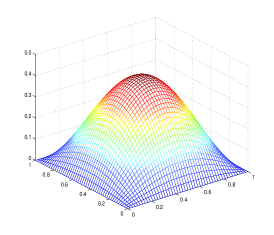
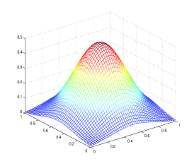
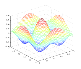
Figure 1: Discrete approx. (left), smooth approx. (center) for the same grid, and pointwise difference between the two (right, notice the vertical axis scale) for nonlinear PDE (11)

5.3 Reaction diffusion equation

A challenging ODE problem which is known to have many solutions is given as in [Mimura(1979)] by :

$$\begin{array}[]{l@{\:}l}\frac{1}{20}\;{u^{\prime\prime}}+\frac{1}{9}\left(35+16u-u^{2}\right)\;u-u\,v=0\hfil\>&\text{on }[0,5],\\ 4{v^{\prime\prime}}-\left(1+\frac{2}{5}v\right)\;v+u\,v=0\hfil\>&\text{on }[0,5],\\ u^{\prime}(0)=u^{\prime}(5)=v^{\prime}(0)=v^{\prime}(5)=0,\hfil\>\\ 0\leq u,v\leq 14\hfil\>&\text{on }[0,5].\end{array}$$ (12)

To ensure numerical stability we scale the domain $[0,5]$ of (12) to $[0,1]$ before applying Method 2, as $\exp(x^{i})$ gets very large for $|x|>1$. Problem (12) involves two functions $u$ and $v$, thus we need to apply Method 2 twice, once for $u$ and once for $v$, in order to obtain smooth approximations for both functions. Note that the SDPR method only needs to be applied once and provides a discrete approximation $(u_{i},v_{i})_{i}$, maximum entropy estimation needs to be applied twice. We apply Method 2 for $F(u,v)=-u_{\lceil\frac{N}{2}\rceil}$ , $N=100$, $w=3$ and $M\in\{10,20,30,50\}$. Solutions for $u$ and $v$ and the derived smooth approximations are pictured in Figure 2 and the errors are reported in Table 5. Even though the average and the maximum pointwise approximation errors are not small, even for large $M$, we observe that the pointwise approximation gets more and more accurate on certain segments of the domain - in this case the third part of the interior, where the third peak of $u$ and $v$ occurs. The pointwise approximation is not good - or does even get worse - near the boundary of $[0,1]$.

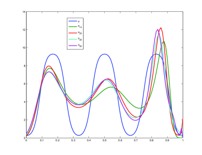
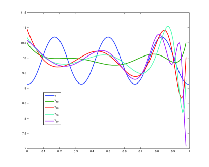
Figure 2: Smooth approx. for $u$ (left) and $v$ (right) for $M\in\{10,20,30,50\}$ for nonlinear ODE (12)

$M$	$\epsilon_{u}^{\max}(M)$	$\bar{\epsilon}_{u}(M)$	$\epsilon_{v}^{\max}(M)$	$\bar{\epsilon}_{v}(M)$
10	4.11	0.0011	2.10	0.1080
20	3.84	0.0143	6.66	0.1371
30	3.48	0.0012	9.61	0.1547
50	3.39	0.0085	23.69	0.2658

Table 5: Errors for nonlinear ODE (12)

5.4 Control of production and consumption

A first example of an optimal control problem is given by

$$\begin{array}[]{lll}\min&-\int_{0}^{T}(1-u(t))x(t)\,dt\\ \text{s.t.}&\dot{x}(t)=u(t)x(t)&\forall t\in\left[0,T\right],\\ &x(0)=x_{0},\\ &0\leq x(t)\leq 1&\forall t\in\left[0,1\right],\\ &0\leq x(t)\leq 10&\forall t\in\left[0,10\right],\end{array}$$ (13)

where $T>1$ fixed. For this simple problem the optimal control law is given by

$$u^{\star}(t)=\begin{cases}1&\text{if }0\leq t\leq T-1,\\ 0&\text{if }T-1<t\leq T.\end{cases}$$

We choose $x_{0}=0.25$, $T=4$ and $N=100$, and apply Method 2 after scaling the domain to $[0,1]$ for $M\in\{5,10,20,30\}$. In this case the objective function $F$ is given by a discretization of the objective function of (13). As in the case of ordinary and partial differential equations, we observe that a fairly good pointwise approximations of both, optimal control law and corresponding trajectory, are obtained on the interior of the domain. See Figure 3.

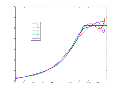
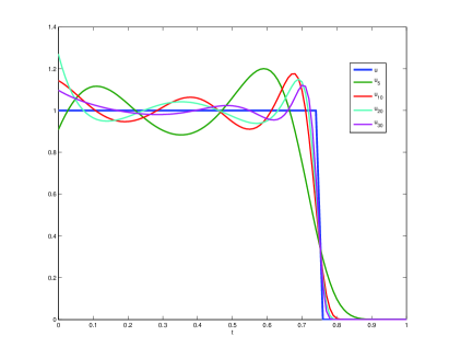
Figure 3: Smooth approx. for $x$ (left) and $u$ (right) for $M\in\{5,10,20,30\}$ for OCP (13).

5.5 The double integrator

Another interesting control problem, which has been discussed in [Lasserre et al.(2008)], is given by

$$\begin{array}[]{lll}\min&T\\ \text{s.t.}&\dot{x}_{1}(t)=x_{2}(t)&\forall\,t\in\left[0,T\right],\\ &\dot{x}_{2}(t)=u(t)&\forall\,t\in\left[0,T\right],\\ &x(0)=x_{0}\in\mathbb{R}^{2},\\ &x(T)=(0,0),\\ &-1\leq u(t)\leq 1&\forall\,t\in[0,T],\\ &-1\leq x_{1}(t),x_{2}(t)\leq 10&\forall\,t\in[0,T].\end{array}$$ (14)

After scaling the domain to $[0,1]$, we apply Method 2 with $N=50$, $\omega=3$, $x_{0}=(0.8,-1)$ and $M\in\{5,10,20,30\}$. Since $T$ is not fixed, it is treated as an additional variable, i.e., we consider the polynomial optimization problem with variable $({x_{1}}_{1},\ldots,{x_{1}}_{N},{x_{2}}_{1},\ldots,{x_{2}}_{N},u_{1},\ldots,u_{N},T)$. We observe that the pointwise approximation of optimal control and trajectories on the interior of the domain gets better and better for increasing moment order, see Figure 4. Note, unlike the moment based method in [Lasserre et al.(2008)] which yields bounds for the optimal value of the control problem, we obtain discrete and smooth approximations to the optimal control and the corresponding trajectories by Method 1 and Method 2, respectively.

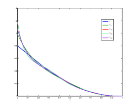
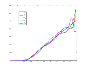
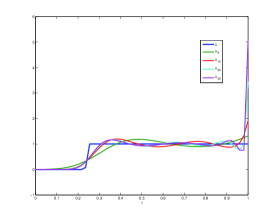
Figure 4: Smooth approx. for $x_{1}$ (left), $x_{2}$ (center) and $u$ (right) for $M\in\{5,10,20,30\}$ forOCP (14).

6 Concluding Remarks

We introduced a novel technique to derive smooth approximations for solutions of systems of differential equations and optimal control problems, which is based on sparse SDP relaxations and the maximum entropy estimation method. As demonstrated on some examples of nonlinear ordinary differential equations, partial differential equations and optimal control problems, this technique is promising to obtain accurate pointwise approximations of a solution of a differential equation on segments of its domain. It would be interesting to characterize regions of the domain of nonlinear differential equations where accurate pointwise approximations can be guaranteed. Another question is whether a different, less restrictive parametrization than (6) allows better pointwise approximations on larger segments of the domain. Of course, other choices of entropy would lead to different results, and it remains a topic of future investigation to analyze, whether or not some choice should be preferred. At this point solving the sparse SDP relaxation is the major computational bottleneck in Method 2. Every improvement for approximation accuracy and efficiency of SDP relaxation techniques for polynomial programs and every improvement for SDP solvers will extend the range of the proposed method.

In order to validate these techniques in the present context of PDEs, a comparison with state-of-the-art numerical methods for solving nonlinear PDEs remains to be done. In particular, the maximum entropy technique should be compared with standard and spline interpolation methods which both provide differentiable approximations that coincide with the discrete solution at each grid point. But, unlike our method, in polynomial interpolation the degree of the polynomial is directly related to the number of grid points. Also, cubic splines are twice differentiable at the grid points, whereas our approximation is smooth. In contrast, and instead of searching for a smooth solution that matches the unknown $u$ at the grid points, one searches for a smooth solution that matches finitely many moments of the associated measure $d\mu=udx$. And so, an interesting feature is to obtain a smooth approximation from a limited number of moments and not from the discrete solution explicitly (still, before using moments, a sufficiently fine discretization is necessary to ensure $m^{\Delta}\approx m$). This method is an attempt to deal with the curse of dimensionality in the numerical analysis of PDEs. Furthermore, we emphasize that the proposed method can be applied to a wide range of problems that encompasses nonlinear partial differential equations and nonlinear optimal control problems. A detailed comparison is however out of the scope of this paper, whose main objective was to pave the way for the development of SDP techniques to solve optimal control design problems for dynamical systems described by polynomial ODEs and PDEs, in the spirit of [Lasserre et al.(2008)].

References

- [Bertsimas et al. (2006)] D. Bertsimas, C. Caramanis, Bounds on linear PDEs via semidefinite optimization, Math. Prog. Ser. A 108:135-158, 2006.
- [Bertsimas et al.(2008)] D. Bertsimas, X.V. Doan, J.B. Lasserre, Approximating integrals of multivariate exponentials: a moment approach, Op. Res. Letters 36:205-210, 2008.
- [Borwein et al.(1991)] J. Borwein, A.S. Lewis, On the convergence of moment problems, Trans. Am. Math. Soc. 325:249-271, 1991.
- [Lasserre et al.(2008)] J. B. Lasserre, D. Henrion, C. Prieur, E. Trélat. Nonlinear optimal control via occupation measures and LMI relaxations, SIAM J. Control Opt. 47:1643-1666, 2008.
- [Lasserre(2006)] J.B. Lasserre, Convergent SDP relaxations in polynomial optimization with sparsity, SIAM J. Opt. 17:822-843, 2006.
- [Lasserre(2007)] J.B. Lasserre, Semidefinite programming for gradient and Hessian computation in maximum entropy estimation, Proc. IEEE Conf. Dec. Control, 2007.
- [Lasserre(2009)] J.B. Lasserre, Moments, positive polynomials and their applications, Imperial College Press, London, 2009.
- [Mevissen et al.(2008)] M. Mevissen, M. Kojima, J. Nie, N. Takayama, Solving partial differential equations via sparse SDP relaxations, Pacific J. Opt. 4:213-241, 2008.
- [Mevissen et al.(2009)] M. Mevissen, K. Yokoyama, N. Takayama, Solutions of polynomial systems derived from the steady cavity flow problem, Proc. Intl. Symp. Symb. Alg. Comp., 2009.
- [Mimura(1979)] M. Mimura, Asymptotic behaviors of a parabolic system related to a planktonic prey and predator model, SIAM J. Appl. Math. 37:499-512, 1979.
- [Waki et al.(2006)] H. Waki, S. Kim, M. Kojima, M. Muramatsu, Sums of squares and semidefinite program relaxations for polynomial optimization problems with structured sparsity, SIAM J. Opt. 17:218-242, 2006.
- [Waki et al.(2005)] H. Waki, S. Kim, M. Kojima, and M. Muramatsu, SparsePOP: a sparse semidefinite programming relaxation of polynomial optimization problems, Dept. Math. Comp. Sci., Tokyo Inst. Tech., Research Report B-414, 2005.