Experimental Realization of the Deutsch-Jozsa Algorithm with a Six-Qubit Cluster State

Abstract

We describe the first experimental realization of the Deutsch-Jozsa quantum algorithm to evaluate the properties of a 2-bit boolean function in the framework of one-way quantum computation. For this purpose a novel two-photon six-qubit cluster state was engineered. Its peculiar topological structure is the basis of the original measurement pattern allowing the algorithm realization. The good agreement of the experimental results with the theoretical predictions, obtained at $\sim$1kHz success rate, demonstrate the correct implementation of the algorithm.

Introduction. – In the last decade, quantum information processing and, in particular, quantum computation, have been conquering increasing interest and importance in the scientific community, supported by the promising theoretical and experimental results obtained. One of the many present efforts is the construction of quantum hardware, which up to now has been realized by following different experimental techniques Kok et al. (2007); Benhelm et al. (2008). In this way, it was then possible to demonstrate the correct functioning of one and two-qubit logic gates as well as the successful implementation of quantum algorithms which strongly show the efficiency of a quantum computer with respect to its classical analogue. Among these, the Deutsch-Jozsa (DJ) algorithm is the first example of the speed-up exhibited by a computer taking advantage of quantum mechanics in the evaluation of a global property of an $n$-bit boolean function Deutsch and Jozsa (1992).

In this Letter we report the realization of the Deutsch-Jozsa algorithm in the framework of the one-way model of quantum computation Raussendorf and Briegel (2001); Briegel et al. (2009), which has already proved successful in the construction of quantum gates such as the controlled-NOT (CNOT) gate Vallone et al. (2008a); Gao et al. (2009); Vallone et al. (2009a) and in the implementation of the Grover Vallone et al. (2008b); Walther et al. (2005); Prevedel et al. (2007); Vallone et al. (2008a) and the Deutsch algorithms Vallone et al. (2008b); Tame et al. (2007). The latter corresponds to the case $n=1$ and is based on the use of four-qubit cluster photon states. Here we get the access to the case $n=2$ by taking advantage of a peculiar two-dimensional two-photon six-qubit cluster state generated by a source of multi-qubit cluster states whose performances have been already demonstrated Ceccarelli et al. (2009); Vallone et al. (2009a). At variance with the simple case $n=1$, the DJ algorithm allows to take advantage of the exponential growing of the computational speed-up for increasing values of $n$, as said. Hence the results presented in this paper are important in that they open the way to the implementation of the DJ algorithm with a still larger number of qubits. Although the DJ algorithm has been implemented before with photons Brainis et al. (2003), our realization represents the first realization with a 2-bit function in the context of measurement-based quantum computation.

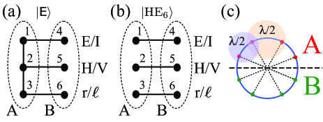
Figure 1: Graphs associtated to (a) the $|{\textsf{E}}\rangle$ cluster and (b) the $|{\rm HE}_{6}\rangle$ hyperentangled state. Qubits 1, 4 are encoded in the E/I momentum, qubits 2, 5 are encoded in polarization (H/V) and qubits 3, 6 in the r/$\ell$ momentum. (c) Annular section of the conical SPDC emission of a Type I phase matched crystal. The source produces the $|{\rm HE}_{6}\rangle$ state over eight spatial modes. Two half wave-plates ($\lambda/2$) with vertical optical axis intercepting three modes of the $A$ photon are used to transform $|{\rm HE}_{6}\rangle$ into the $|{\textsf{E}}\rangle$ state.

Realization pattern for the Deutsch-Jozsa algorithm. – Let us briefly recall the generalized version of the Deutsch algorithm Deutsch and Jozsa (1992), where a set of $n$ qubits constitutes the input of a black box, usually known as the Oracle, which implements the $n$-bit boolean function $f(x)$ such that $f:\{0,1\}^{n}\rightarrow\{0,1\}$. The aim of the DJ algorithm is to determine whether the function evaluated by the oracle is constant or balanced; a function $f$ is said to be balanced if it is equal to $0$ when calculated in half of the possible values of $x$ and equal to $1$ when the remaining allowed values for $x$ are taken into account. Classically, $2^{n-1}+1$ queries to the oracle are necessary to solve the problem while, in the frame of quantum mechanics, the answer comes with one single query. Consequently, the greater is the number $n$ of qubits involved, the more evident is the difference in the performances of the quantum computer with respect to its classical counterpart. The initial state of the system is $|0\rangle\otimes|0\rangle\otimes\cdots\otimes|0\rangle=|0\rangle^{\otimes n}$ and an ancillary qubit in the state $|1\rangle$ is added to the $n$ input qubits. The operation performed by the oracle is given by $(\textsf{H}^{\otimes n}\otimes\textsf{H})U_{f}(\textsf{H}^{\otimes n}\otimes\textsf{H})$, where H is the Hadamard gate; the unitary operator $U_{f}$ acts on the states of the computational basis so that $U_{f}|x\rangle|y\rangle=|x\rangle|y\oplus f(x)\rangle$. The final state is found to be $\bigl{(}\frac{1}{2^{n}}\sum_{x,y=0}^{2^{n}-1}(-1)^{f(x)+x\cdot y}|y\rangle\bigr{)}|1\rangle$. Measuring the state of the $n$ qubits in the computational basis leads to the conclusion: if we get the state $|0\rangle^{\otimes n}$ the function $f$ is constant, otherwise it is balanced, as seen from the above expression for the final state of the global system. Moreover, the measurement of the ancillary qubit in the computational basis is expected to always return the $|1\rangle$ state.

We now go into the details of the proposed experimental realization of the DJ algorithm for a function acting on $n=2$ bits. In this case, the boolean function which we are interested in is such that $f:~{}\{0,1\}^{2}\rightarrow\{0,1\}$. The function $f$ can be calculated in its four arguments $x=0,1,2,3$, with $x=2x_{1}+x_{0}$ and $x_{0},x_{1}=0,1$. Among the 16 possible functions of this kind, we focus our attention on the balanced function $f_{B}$, such that $f_{B}(0)=f_{B}(3)=0$, $f_{B}(1)=f_{B}(2)=1$, and on the constant function $f_{C}$ for which we have that $f_{C}(x)=0$ for every allowed value of $x$. We thus identify the state $|x\rangle_{Q}=|x_{1}\rangle_{\overline{1}}|x_{0}\rangle_{\overline{2}}$ as the input entering the oracle. In the former expression the subscripts $\overline{1}$ and $\overline{2}$ refer to logical qubits. As we know, the implementation of the DJ algorithm requires an additional ancillary qubit in the initial state $|y\rangle_{A}\equiv|y\rangle_{\overline{3}}$ , where $\overline{3}$ is the logical qubit associated to the ancilla. For the previously defined functions we have that $U_{f_{C}}=\openone$ and $U_{f_{B}}=\textsc{Cnot}_{\bar{1}\bar{3}}\textsc{Cnot}_{\bar{2}\bar{3}}$, respectively.

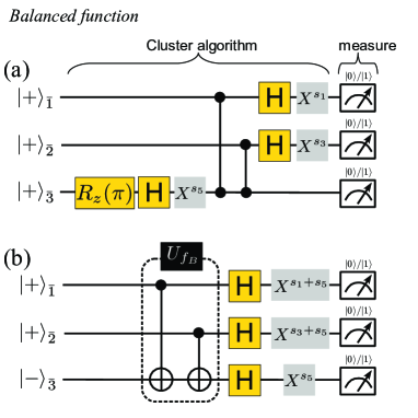
Figure 2: Balanced function: (a) algorithm realized according to the pattern of single-qubit measurements and (b) equivalent circuit implementing the DJ algorithm for $n=2$. Gray gates represent Pauli errors.

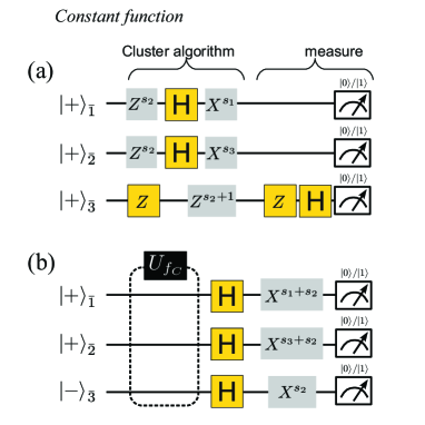
Figure 3: Constant function: (a) algorithm realized according to the pattern of single-qubit measurements and (b) equivalent circuit implementing the DJ algorithm for $n=2$. Gray gates represent Pauli errors.

In the framework of one-way quantum computing, the starting point of any computation is the construction of a multi-qubit cluster state; successively, the choice of a sequence of single-qubit measurements determines the program to be executed on the quantum computer. For a review on graph and cluster states and their use for one-way computing see Raussendorf and Briegel (2001); Briegel et al. (2009); Hein et al. (2006); Vallone et al. (2008b). Let us start from the identification of the appropriate cluster state allowing the realization of the DJ algorithm in the present work: Fig. 1(a) shows the graph corresponding to a two-dimensional six-qubit cluster state where the numbered vertices stand for physical qubits. These qubits are equally distributed among two photons, labeled as $A$ and $B$: qubits $1$, $2$ and $3$ belong to photon $A$ and interact by two controlled-Z gates represented by vertical connections on the graph, while qubits $4$, $5$ and $6$ are associated to photon $B$. As usual in the one-way model, it can be useful to think of the distinct horizontal qubits as “the original [logical] qubit at different times” Nielsen (2004); indeed, we identify the logical qubits $\overline{1}$ and $\overline{2}$ with physical qubits $1$, $4$ and $3$, $6$, respectively. The ancillary qubit $\overline{3}$ is represented by qubits $2$ and $5$. The “E cluster” just described is our quantum computer; we can show that the choice of the measurement sequence for the two qubits associated to the ancilla leads to the evaluation of both the balanced $f_{B}$ and the constant $f_{C}$ functions. This implies that, in the E cluster, qubits $2$ and $5$ play the role of the oracle, while the remaining qubits constitute the tools we have at our disposal to discriminate between a balanced and a constant function. To better understand this feature it is useful to consider the circuit representations associated to the realization of the two considered global properties of the 2-bit boolean function $f$.

The proposed measurement configurations are the following:

1. balanced function - By measuring qubits $1$, $3$ and $5$ in the bases $B_{1}(0)$, $B_{3}(0)$ and $B_{5}(\pi)$ we implement, at the logical level, the two Cnot gates ($U_{f_{B}}$) needed to implement the oracle function $f_{B}$ (see Fig. 2). Then we proceed with the measurement of the output qubits $4$, $6$ and $2$ in the bases $C_{4}^{|0\rangle}$, $C_{6}^{|0\rangle}$ and $C_{2}^{|0\rangle}$.

2. constant function - We measure qubits $1$, $3$ and $2$ in the bases $B_{1}(0)$, $B_{3}(0)$ and $C_{2}^{|0\rangle}$. These operations implement, at the logical level, the identity gate $U_{f_{C}}$ needed to implement the oracle function $f_{C}$ (see Fig. 3). Then we read the result of the computation on the output qubits $4$, $6$ and $5$ by measuring them in the bases $C_{4}^{|0\rangle}$, $C_{6}^{|0\rangle}$ and $B_{5}(\pi)$.

We define $B_{j}(\alpha)=\{|\alpha_{+}\rangle_{j},|\alpha_{-}\rangle_{j}\}$ with $|\alpha_{\pm}\rangle_{j}=\frac{1}{\sqrt{2}}(|0\rangle\pm e^{-i\alpha}|1\rangle_{j})$, while $C_{j}^{|0\rangle}=\{|0\rangle_{j},|1\rangle_{j}\}$ is the computational basis for the Hilbert space associated to qubit $j$. The above sequences of single-qubit measurement lead us to the circuits shown in Fig. 2 and 3; in particular, we can see the elements of the circuit realizing the unitary transformation $U_{f}$ for the balanced function $f_{B}$ and the constant function $f_{C}$, as well as single-qubit Pauli gates. Here and in the following we indicate with $Z$ ($X$) the Pauli matrix $\sigma_{z}$ ($\sigma_{x}$). For a given basis $B_{j}(\alpha)$, we introduce the quantity $s_{j}$ whose value is $0$ ($1$) if the measurement result is equal to $|\alpha_{+}\rangle_{j}$ ($|\alpha_{-}\rangle_{j}$) and equivalently for the $C_{j}^{|0\rangle}$ basis. According to the algorithm, we will expect, as outputs, the state $|1\oplus s_{1}\oplus s_{5}\rangle_{\bar{1}}|1\oplus s_{3}\oplus s_{5}\rangle_{\bar{2}}|1\oplus s_{5}\rangle_{\bar{3}}$ for the balanced and $|s_{1}\oplus s_{2}\rangle_{\bar{1}}|s_{2}\oplus s_{3}\rangle_{\bar{2}}|1\oplus s_{2}\rangle_{\bar{3}}$ for the constant function. In the previous expressions we take into account the feed-forward corrections of the Pauli errors.

Experimental preparation of the cluster state. – Referring to Fig. 1, the two-dimensional cluster state $|{\textsf{E}}\rangle$ is obtained from a six-qubit hyperentangled state Vallone et al. (2009b), $|{\rm HE}_{6}\rangle$, whose graph is shown in Fig. 1(b) Ceccarelli et al. (2009); Vallone et al. (2009b). Our experimental setup adopts a source of two-photon states based on a Spontaneous Parametric Down-Conversion (SPDC) process where the two particles are entangled at the same time in the polarization and in two linear momentum degrees of freedom (DOFs). By a proper interferometric setup Vallone et al. (2009a) it is possible to measure the two spatial DOFs; these variables, labeled as the “right/left” momentum ($r/\ell$) and the “external/internal” momentum ($E/I$), are both associated to each of the eight modes on which the two photons are emitted. A detailed description of the experimental setup, enabling the transformation from the six-qubit hyperentangled state $|{\rm HE}_{6}\rangle$ into a linear cluster state, can be found in recent papers Ceccarelli et al. (2009); Vallone et al. (2009a). It is interesting to note that the transition from the one-dimensional linear cluster state to the E cluster considered here is entirely determined by the choice of the controlled-$\sigma_{z}$ (CZ) operations corresponding to the vertical links in the graph (see Fig. 1(a)). These gates are optically implemented between couples of qubits belonging to the same photon. The graph associated to the six-qubit cluster state $|{\textsf{E}}\rangle$ exhibits two links between qubits $1$ and $2$ (encoded in the $E/I$ momentum DOF and in polarization, respectively) and between qubits $2$ and $3$ (with qubit 3 encoded in the $r/\ell$ momentum DOF), hence the corresponding $\textsf{CZ}_{12}$ and $\textsf{CZ}_{23}$ logic gates only involve qubits belonging to photon $A$, as already noticed above. The optical implementation of the two controlled-Z gates is realized by means of two half-wave plates, as shown in Fig. 1(c).

In order to give an explicit expression for the six-qubit cluster state produced in the present experiment we point out that the experimental hyperentangled state, which we label as $|\widetilde{\rm HE}_{6}\rangle$, does not coincide with the hyperentangled state $|{\rm HE}_{6}\rangle$ corresponding to the graph in Fig. 1(a) and instead satisfies the relation

$$\begin{split}|\widetilde{\rm HE}_{6}\rangle&=\textsf{H}_{4}Z_{5}\textsf{H}_{5}X_{6}\textsf{H}_{6}|{\rm HE}_{6}\rangle=\\ &=\frac{1}{\sqrt{2}}(|00\rangle_{14}+|11\rangle_{14})\otimes\frac{1}{\sqrt{2}}(|00\rangle_{25}-|11\rangle_{25})\otimes\\ &\quad\otimes\frac{1}{\sqrt{2}}(|01\rangle_{36}+|10\rangle_{36}),\end{split}$$ (1)

where $\textsf{H}_{j}$ is the Hadamard gate on qubit $j$ and $X_{j}$ ($Z_{j}$) is the $\sigma_{x}$ ($\sigma_{z}$) gate on the corresponding qubit. For the E cluster represented by the graph in Fig. 1(a) we can write that

$$|{\textsf{E}}\rangle=\textsf{CZ}_{12}\textsf{CZ}_{23}|{\rm HE}_{6}\rangle.$$ (2)

Combining Eq. (2) with Eq. (1) we get

$$\begin{split}|\widetilde{\textsf{E}}\rangle&=\textsf{CZ}_{12}\textsf{CZ}_{23}|\widetilde{\rm HE}_{6}\rangle=\textsf{H}_{4}Z_{5}\textsf{H}_{5}X_{6}\textsf{H}_{6}|{\textsf{E}}\rangle=\\ &=\frac{1}{2}(|EE\rangle|\phi^{-}\rangle_{\pi}|r\ell\rangle+|EE\rangle|\phi^{+}\rangle_{\pi}|\ell r\rangle\>+\\ &\quad+|II\rangle|\phi^{+}\rangle_{\pi}|r\ell\rangle+|II\rangle|\phi^{-}\rangle_{\pi}|\ell r\rangle)\end{split}$$ (3)

for the six-qubit two-photon E cluster state generated in the laboratory. In the above expression the states $|\phi^{+}\rangle_{\pi}$ and $|\phi^{-}\rangle_{\pi}$ are the two polarization Bell states. As usual Vallone et al. (2008a); Walther et al. (2005); Prevedel et al. (2007), we refer to $|{\textsf{E}}\rangle$ and $|\widetilde{\textsf{E}}\rangle$ as the state in the “cluster” and “laboratory” basis, respectively. As shown in Fig. 1(c) we transform the hyperentangled state $|\widetilde{\rm HE}_{6}\rangle$ into the cluster state $|\widetilde{\textsf{E}}\rangle$ by applying two CZ operations.

Experimental results. – In order to characterize the generated $|\widetilde{\textsf{E}}\rangle$ state we measured the witness operator $\mathcal{W}=3-2(\prod^{3}_{k=1}\frac{\widetilde{g}_{2k}+1}{2}+\prod^{3}_{k=1}\frac{\widetilde{g}_{2k-1}+1}{2})$ Tóth and Gühne (2005a) (see Ceccarelli et al. (2009) for the definition of the $\widetilde{g}_{i}$). We found $\langle\mathcal{W}\rangle=-0.333\pm 0.002$, demonstrating a genuine six-qubit entanglement Tóth and Gühne (2005b). Since it is possible to show Tóth and Gühne (2005a); Vallone et al. (2007) that the fidelity $F$ satisfies the relation $F\geq\frac{1}{2}(1-\langle\mathcal{W}\rangle)$, a lower bound for the fidelity is easily found:

$$F\geq 0.667\pm 0.001.$$ (4)

Let’s now turn to the DJ algorithm. We performed the sets of single-qubit measurements stated above and found the results presented in Table 1: here we show the probabilities of the outputs of the computation when no Pauli errors are present (No-FF). This corresponds to consider only the case where $s_{1}=s_{3}=s_{5}=0$ for the balanced function and $s_{1}=s_{2}=s_{3}=0$ for the constant function. We also show the results obtained by considering all possible outputs and applying the feed-forward (FF) operations correcting the Pauli errors (see also Figs. 2 and 3). It is worth noting that, since the output of the computation is read in the $\{|0\rangle,|1\rangle\}$ basis, the FF is a relabeling feed-forward, i.e. “the earlier measurement determines the meaning of the final readout” (see “Grover’s search algorithm” section of Walther et al. (2005) or the end of section II in Vallone et al. (2008b)).

It is also important to notice that the physical qubits constituting the $|\widetilde{\textsf{E}}\rangle$ cluster were actually measured in the appropriate laboratory basis, which differs from the cluster basis when a single-qubit gate acts on the considered qubit; referring to Eq. (3), this corresponds to the case of qubits $4$, $5$ and $6$.

Table 1: Experimental probabilities of the obtained output states for balanced and constant function, with (FF) or without (no-FF) feed-forward. We indicate in bold character the data corresponding to the expected outputs.

	$f_{B}$: Balanced		$f_{C}:$ Constant
Output	No-FF$(\%)$	FF$(\%)$	No-FF$(\%)$	FF$(\%)$
$|000\rangle$	$0.8\pm 0.1$	$0.9\pm 0.1$	$0.7\pm 0.1$	$0.9\pm 0.1$
$|001\rangle$	$2.7\pm 0.2$	$2.6\pm 0.1$	${\bf 77.5\pm 0.5}$	${\bf 75.2\pm 0.2}$
$|010\rangle$	$1.4\pm 0.2$	$1.4\pm 0.2$	$1.2\pm 0.1$	$1.4\pm 0.1$
$|011\rangle$	$15.5\pm 0.5$	$14.1\pm 0.1$	$3.5\pm 0.2$	$3.4\pm 0.1$
$|100\rangle$	$1.3\pm 0.2$	$1.0\pm 0.1$	$1.2\pm 0.1$	$1.0\pm 0.1$
$|101\rangle$	$2.4\pm 0.2$	$3.4\pm 0.1$	$13.5\pm 0.4$	$14.1\pm 0.2$
$|110\rangle$	$0.4\pm 0.1$	$1.4\pm 0.1$	$0.4\pm 0.1$	$1.4\pm 0.1$
$|111\rangle$	${\bf 75.5\pm 0.6}$	${\bf 75.2\pm 0.2}$	$2.0\pm 0.2$	$2.6\pm 0.1$

The experimental results are in good agreement with the theoretical predictions for both functions. The main discrepancy resides on the output probabilities of the states $|011\rangle$ for $f_{B}$ and $|101\rangle$ for $f_{C}$. These states differ from the expected outputs in the value of the logical qubit $\bar{1}$. This is mainly due to the non perfect interference visibility associated to the E/I momentum DOF ($V\sim 70\%$). We attribute this to the difficulties in obtaining a perfect mode matching in the second interferometer (see Vallone et al. (2009a) for more details).

Conclusions. – We have presented an all-optical implementation of the DJ algorithm for $n=2$ qubits. For this purpose, by taking advantage of the generation of a six-qubit two-photon hyperentangled state, we created a novel, high fidelity, two-dimensional six-qubit cluster state that represents the first step for the realization of the algorithm as a one-way quantum computation. We were then able to evaluate a two-bit balanced function as well as a constant one and to discriminate between them in one single run of the executed program, in contrast to the three runs needed with a classical computer. The correct output is identified at a frequency of almost 1kHz without feed-forward, a result which overcomes by several orders of magnitude what can be achieved with a six-photon cluster state, according to the current optical technology. By using all possible detection outputs and applying the feed-forward corrections we could obtain a frequency 8 times larger. Note that our experiment was actually performed with four detectors Vallone et al. (2009a). In order to consider all the possible outcomes at the same time we would need 16 detectors.

The experimental results demonstrate the correctness of the proposed algorithm implementation and represent the first proof of such a computation with a two-bit function in the framework of the one-way model.