Unconventional Néel and dimer orders in a spin-$\frac{1}{2}$ frustrated ferromagnetic chain with easy-plane anisotropy

Abstract

We study the ground-state phase diagram of a one-dimensional spin-$\frac{1}{2}$ easy-plane XXZ model with a ferromagnetic nearest-neighbor (NN) coupling $J_{1}$ and a competing next-nearest-neighbor (NNN) antiferromagnetic coupling $J_{2}$ in the parameter range $0<J_{2}/|J_{1}|<0.4$. When $J_{2}/|J_{1}|\lesssim 1/4$, the model is in a Tomonaga-Luttinger liquid phase which is adiabatically connected to the critical phase of the XXZ model of $J_{2}=0$. On the basis of the effective (sine-Gordon) theory and numerical analyses of low-lying energy levels of finite-size systems, we show that the NNN coupling induces phase transitions from the Tomonaga-Luttinger liquid to gapped phases with either Néel or dimer order. Interestingly, these two types of ordered phases appear alternately as the easy-plane anisotropy is changed towards the isotropic limit. The appearance of the antiferromagnetic (Néel) order in this model is remarkable, as it is strongly unfavored by both the easy-plane ferromagnetic NN coupling and antiferromagnetic NNN coupling in the classical-spin picture. We argue that emergent trimer degrees of freedom play a crucial role in the formation of the Néel order.

I Introduction

The search for novel orders arising from geometric frustration and quantum fluctuations in low-dimensional quantum spin systems has been a subject of intensive theoretical and experimental research. One-dimensional (1D) systems offer particularly ideal grounds for theoretical studies, as powerful non-perturbative methods are available (for a review, see, for example, Ref. Lecheminant05, ). A prototypical example hosting a variety of fascinating phenomena is the spin-$\frac{1}{2}$ frustrated chain with the nearest-neighbor (NN) and next-nearest-neighbor (NNN) exchange interactions:

$$H=\sum_{m=1}^{2}\sum_{j=1}^{L}J_{m}\left(S^{x}_{j}S^{x}_{j+m}+S^{y}_{j}S^{y}_{j+m}+\Delta S^{z}_{j}S^{z}_{j+m}\right).$$ (1)

Here, $\bm{S}_{j}=(S^{x}_{j},S^{y}_{j},S^{z}_{j})$ is a spin-$\frac{1}{2}$ operator at the site $j$, and $\Delta$ is an XXZ anisotropy. The model has frustration as long as the NNN coupling $J_{2}$ is antiferromagnetic, irrespective of the sign of $J_{1}$.

Much of recent interest in the model (1) has been focused on the case when ferromagnetic (FM) $J_{1}<0$ and antiferromagnetic (AFM) $J_{2}>0$ compete. The growing interest was triggered by experimental studies of various quasi-1D edge-sharing cupratesHase04 ; Masuda05 ; Enderle05 ; Drechsler07 which can be modelled by the Hamiltonian (1). Theoretical studies have uncovered a rich phase diagram of the model in a magnetic field, which includes the vector chiral phase, spin nematic, and various other multipolar liquids.Chubukov91 ; Kolezhuk05 ; Heidrich06 ; Vekua07 ; Kecke07 ; Hikihara08 ; Sato09 ; Sudan09 ; Heidrich09 Even without a magnetic field, the model (1) shows a variety of phases depending on the values of the exchange anisotropy $\Delta$ and the frustration parameter $J_{2}/|J_{1}|$. Earlier studies have discussed the dimer orderTonegawa90 ; Somma01 and the stability of the vector chiral orderFSSO08 ; Sirker09 in the easy-plane case $0\leq\Delta<1$, and the partial ferromagnetismTonegawa90 in the easy-axis case $\Delta>1$. In this paper we show that the phase diagram of the $J_{1}$-$J_{2}$ chain with easy-plane XXZ anisotropy, Eq. (1), exhibits unexpectedly complicated and interesting phase structure, where Néel and dimer ordered phases alternate more than twice, near a FM critical point $(J_{2}/|J_{1}|,\Delta)=(0.25,1)$. Our analysis is based on the combination of bosonization and numerical analysis of finite-size energy spectrum, which has been proven successful in the study of many 1D quantum spin models including the model (1) with the antiferromagnetic NN coupling.

The ground-state phase diagram of the anisotropic $J_{1}$-$J_{2}$ spin chain (1) is well understood in the antiferromagnetic case, $J_{1}>0$ and $J_{2}>0$ (see, e.g., Refs. Majumdar69, ; Haldane80, ; Haldane82, ; Okamoto92, ; Nomura94, ; White96, ; Nersesyan98, ; Hikihara01, ). For small $J_{2}/J_{1}$ and with easy-plane anisotropy $\Delta<1$, the model is in a gapless phase which is described as a Tomonaga-Luttinger liquid (TLL). The gapless TLL phase has instabilities towards antiferromagnetic (Néel) order and dimerization (as exemplified by the exact singlet dimer ground stateMajumdar69 for $J_{2}/J_{1}=1/2$ and $\Delta>-1/2$). Both Néel and dimer ordered phases are gapped. The Néel order is induced by easy-axis anisotropy $\Delta>1$, while the dimer order appears when $J_{2}/J_{1}$ is larger than some critical value ($\approx 0.24$ at $\Delta=1$). HaldaneHaldane80 ; Haldane82 showed that the quantum phase transitions to these ordered phases can be understood in a unified way within the sine-Gordon (SG) model which is obtained by bosonizing the Hamiltonian (1). The two types of orders arise as a bosonic field is locked at two distinct values by the cosine potential coming from the Umklapp scattering of Jordan-Wigner fermions. It is also worth noting that, for large $J_{2}/J_{1}$, a vector chiral ordered phase with gapless excitations appears for a certain range of easy-plane anisotropy,Nersesyan98 ; Hikihara01 while the dimer ordered phase persists in the isotropic case $\Delta=1$.White96

In this paper, we apply the SG formalism of HaldaneHaldane80 ; Haldane82 to the frustrated ferromagnetic spin chain (1). Our starting point is the FM $J_{1}$-only chain with easy-plane anisotropy $0\leq\Delta<1$. In this case the system is a TLL whose properties are understood in great detail from the Bethe ansatz and the bosonization. In particular, the parameters in the effective SG theory are known exactly.Lukyanov98 ; Lukyanov03 According to these exact results, rather interestingly, there occurs a series of sign changes in the coupling of the cosine potential, as a function of the anisotropy $\Delta$. In the $J_{1}$ XXZ chain, the cosine potential is irrelevant in the renormalization-group (RG) sense and does not make any significant impact on the long-distance properties. However, it is made relevant by large enough $J_{2}$ coupling, and as a result we observe alternating appearance of Néel and dimer ordered phases, as the exchange anisotropy is changed towards the FM critical point $(J_{2}/|J_{1}|,\Delta)=(0.25,1)$. We determine the phase boundaries accurately using finite-size scaling analysis of discrete energy levels, the so-called level spectroscopy method,Okamoto92 ; Nomura94 ; Nomura95 which combines the SG theory with the numerical exact diagonalization. The appearance of the antiferromagnetic spin ordering in the $z$ direction is particularly counterintuitive; on the classical level, such spin configuration is strongly unfavored by the easy-plane FM $J_{1}$ coupling as well as by the AF $J_{2}$ coupling. We analyze the correlations and the reduced density matrices of the ground state in the Néel phase using the infinite time-evolving block decimation (iTEBD) algorithm,Vidal07 a numerical method which can directly address physical quantities in the thermodynamic limit. We will then argue that emergent trimer degrees of freedom play a crucial role in the formation of the Néel ordered state.

The present study focuses on the region with $J_{2}/|J_{1}|\lesssim 0.4$. The analysis of the region with larger $J_{2}/|J_{1}|$ is also done by iTEBD and will be reported elsewhere.FSO It is found that for $J_{2}/|J_{1}|>1/4$, the vector chiral ordered phase with gapless excitations is robust up to a very weak anisotropy $\Delta\approx 1$ and appears in a wide range of the parameter space. This is in contrast to the antiferromagnetic $J_{1}$-$J_{2}$ model, where the vector chiral ordered phase has been identifiedHikihara01 only for large $J_{2}/J_{1}(\gtrsim 1.2)$.

II Formalism

II.1 Effective field theory

We first consider the case $J_{2}=0$, i.e., the easy-plane XXZ chain with $J_{1}<0$. We parametrize the exchange anisotropy as

$$\Delta=\cos(\pi\eta),\quad 0<\eta\leq\frac{1}{2}.$$ (2)

In this parameter range, the model is in the gapless TLL phase. In the bosonization formalism (for a review, see, e.g., Refs. Giamarchi04, ; Gogolin98, ), its low-energy effective theory is the quantum SG theory defined by the Hamiltonian density

$${\cal H}=\frac{v}{2}\left[K\left(\frac{d\theta}{dx}\right)^{2}+\frac{1}{K}\left(\frac{d\phi}{dx}\right)^{2}\right]-\frac{v\lambda}{2\pi}\cos(\sqrt{16\pi}\phi),$$ (3)

where the bosonic field $\phi$ and its dual counterpart $\theta$ obey the commutation relation $[\phi(x),\theta(y)]=-(i/2)[1+\mathrm{sgn}(x-y)]$, and the lattice constant is set to unity. The TLL parameter $K$ and the spin velocity $v$ are given by

$$K=\frac{1}{2\eta},\quad v=|J_{1}|\frac{\sin(\pi\eta)}{2(1-\eta)}.$$ (4)

The cosine potential in Eq. (3) has scaling dimension $4K$ and is irrelevant in the XXZ chain with the exchange anisotropy (2). We keep the cosine term because it will drive the phase transitions from the TLL to the Néel and dimer ordered phases in the presence of the frustrated NNN coupling $J_{2}>0$. When $J_{2}=0$, the exact value of the coupling constant $\lambda$ is known to beLukyanov98 ; Lukyanov03 ; Furusaki05

$$\lambda_{0}=-\frac{4}{\pi}\sin\!\left(\frac{\pi}{\eta}\right)\left[\Gamma\!\left(\displaystyle\frac{1}{\eta}\right)\right]^{2}\left[\frac{\Gamma\!\left(\displaystyle 1+\frac{\eta}{2-2\eta}\right)}{\sqrt{4\pi}\,\Gamma\!\left(\displaystyle 1+\frac{1}{2-2\eta}\right)}\right]^{\frac{2}{\eta}-2}\!\!,$$ (5)

where the normalization condition on the zero-temperature correlator of vertex operators,

$$\langle e^{i\mu\phi(x)}e^{-i\mu\phi(x^{\prime})}\rangle=|x-x^{\prime}|^{-K\mu^{2}/2\pi},\quad|x-x^{\prime}|\gg 1,$$ (6)

is assumed. Notice that $\lambda_{0}$ vanishes at $\eta=1/n$, i.e.,

$$\Delta=\cos\left(\pi/n\right),\quad n=3,4,\dots~{}.$$ (7)

At these points, the XXZ model is invariant under the action of the loop algebra $sl_{2}$, leading to some non-trivial degeneracies in the energy spectrum.Deguchi01 ; Bortz09 We will observe one example of such degeneracies in our numerical result later.

The spin operators of the original lattice model (1) are expressed asnote_Sp

$$S_{j}^{z} = \frac{1}{\sqrt{\pi}}\frac{d\phi}{dx}+(-1)^{j}a\cos(\sqrt{4\pi}\phi)+\dots,$$ (8)

$$S_{j}^{+} = e^{i\sqrt{\pi}\theta}\left[b_{0}+(-1)^{j}b_{1}\cos(\sqrt{4\pi}\phi)+\dots\right],$$ (9)

where $a$, $b_{0}$, and $b_{1}$ are non-universal constants.Lukyanov97 ; Lukyanov99 ; Hikihara98 Similarly, the staggered part of the NN exchange energy is given by

$$\bm{S}_{j}\cdot\bm{S}_{j-1}-\bm{S}_{j}\cdot\bm{S}_{j+1}=c(-1)^{j}\sin(\sqrt{4\pi}\phi)+\ldots,$$ (10)

where $c$ is another non-universal constant.

Including the NNN coupling $J_{2}>0$ changes the parameters ($v$, $\lambda$, and $K$) in the effective theory (3). A perturbative calculation using (8) and (9) yields the renormalized TLL parameter for $J_{2}/|J_{1}|\ll 1$,

$$K=K_{0}\left[1-\frac{J_{2}}{v_{0}}\left(\frac{2\pi b_{1}^{2}}{K_{0}}+\frac{K_{0}\Delta}{\pi}\right)\right],$$ (11)

where $K_{0}$ and $v_{0}$ are the values of $K$ and $v$ at $J_{2}=0$ given in Eq. (4). This indicates that $K$ decreases as $J_{2}/|J_{1}|$ increases. As long as $K$ is larger than 1/2, the cosine term is irrelevant and the system is in the TLL phase. As $J_{2}/|J_{1}|$ is further increased, the cosine term in Eq. (3) will eventually become relevant ($4K<2$). The positive and negative values of $\lambda$ will then trigger the Néel and dimer orders, respectively, as one can see from Eqs. (8) and (10). We analyze such ordering transitions through a combination of the RG analysis of the SG model (3) and the finite-size spectra obtained from numerical exact diagonalization.

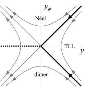
Figure 1: RG flow diagram of the sine-Gordon theory (3). The thick solid lines indicate the Kosterliz-Thouless-type transitionsKosterlitz73 between the TLL and the two ordered phases. The dotted line indicates the Gaussian transition between the two ordered phases.

II.2 Renormalization group flow

We discuss the RG flows of the SG theory (3) by varying a short-distance cutoff $\alpha$. To this end, it is convenient to parametrize

$$\alpha=\alpha_{0}e^{l},\quad K=\frac{1}{2}+\frac{y(l)}{4},\quad\lambda=\frac{y_{\phi}(l)}{\alpha^{2}},$$ (12)

where $\alpha_{0}$ is the initial cutoff. Under an infinitesimal change $l\to l+dl$, the dimensionless parameters $y(l)$ and $y_{\phi}(l)$ change according to the RG equations

$$\frac{dy(l)}{dl}=-y_{\phi}^{2}(l),\quad\frac{dy_{\phi}(l)}{dl}=-y_{\phi}(l)y(l).$$ (13)

The RG flow diagram is drawn in Fig. 1. When $0<y<|y_{\phi}|$, the cosine potential finally vanishes, and the system is described as the TLL. The transitions from the TLL to the Néel and dimer phases occur along the half lines $y_{\phi}=+y$ and $y_{\phi}=-y$ with $y>0$ (thick solid lines), respectively. The transition between the two ordered phases occurs along the Gaussian fixed line $y_{\phi}=0$ with $y<0$ (dotted line).

II.3 Level spectroscopy

On the basis of the RG flow diagram of the SG model in Fig. 1, Okamoto and NomuraOkamoto92 ; Nomura94 ; Nomura95 developed a simple numerical method which allows to determine the phase transition lines precisely. The key idea of this method is to look at the lowest excited states in the three different phases. Under the periodic boundary condition, the eigenstates of a finite-size system of length $L$ are labeled by the magnetization $S^{z}=\sum_{j}S_{j}^{z}$, the wave number $q=2\pi k/L~{}(k\in\mathbb{Z})$, the (bond-centered) parity $P=\pm 1$, and the spin reversal $T=\pm 1$. In the parameter region of our interest, the ground state (with energy $E_{0}$) of the model (1) is in the sector $(S^{z}=0,q=0,P=+1,T=+1)$ when $L$ is even. In the TLL phase, the first excited state (with energy $E_{\rm S}$) is in the sector $(S^{z}=\pm 1,q=0,P=+1)$. In the Néel and dimer phases, pseudo ground states (with energies $E_{\rm N}$ and $E_{\rm D}$) appear in the sectors $(S^{z}=0,q=\pi,P=-1,T=-1)$ and $(S^{z}=0,q=\pi,P=+1,T=+1)$, respectively, reflecting the two-fold ground-state degeneracy in the thermodynamic limit. One can expect that the transitions between the three phases can be detected by observing crossing of these energy levels.

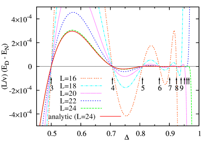
Figure 2: (color online) Energy difference $(L/v)(E_{\mathrm{D}}-E_{\mathrm{N}})$ in the unfrustrated case $J_{2}=0$. The arrows indicate the “special” points in Eq. (7) with $n=3,4,\dots$, where $\lambda$ changes the sign.

This expectation can be justified by a detailed analysis of the finite-size spectra of the sine-Gordon theory. Nomura95 See Appendix for details. Here we briefly mention the basic idea. The excitation energy $\Delta E_{\rm S}:=E_{\rm S}-E_{0}$ is associated with the operator $S_{j}^{\pm}\sim e^{\pm i\sqrt{\pi}\theta(x)}$. The excitation energies $\Delta E_{\rm N}:=E_{\rm N}-E_{0}$ and $\Delta E_{\mathrm{D}}:=E_{\mathrm{D}}-E_{0}$ are associated with the order operators $(-1)^{j}S_{j}^{z}\sim\cos(\sqrt{4\pi}\phi)$ and $(-1)^{j}(S_{j}^{+}S_{j+1}^{-}+\rm{h.c.})\sim\sin(\sqrt{4\pi}\phi)$, respectively. From the correspondence between the spectra and the operators, one obtains

$$\Delta E_{\mathrm{S}}=\frac{2\pi v}{L}\left(\frac{1}{2}-\frac{y(l)}{4}\right),$$ (14a)

$$\Delta E_{\mathrm{N}}=\frac{2\pi v}{L}\left(\frac{1}{2}+\frac{y(l)}{4}-\frac{y_{\phi}(l)}{2}\right),$$ (14b)

$$\Delta E_{\mathrm{D}}=\frac{2\pi v}{L}\left(\frac{1}{2}+\frac{y(l)}{4}+\frac{y_{\phi}(l)}{2}\right),$$ (14c)

where $l$ is related to the system size $L$ by $e^{l}=L/2\pi$. One can see that the crossing of $E_{\rm S}$ and $E_{\rm N}$ occurs when $y(l)=y_{\phi}(l)$, corresponding to the TL-Néel transition in Fig. 1. Similarly, $E_{\rm S}=E_{\rm D}$ corresponds to the TL-dimer transition. Using the formula $L(E_{\rm D}-E_{\rm N})=2\pi vy_{\phi}(l)$, one can observe the running coupling constant, in particular, its sign change. In Fig. 2, $(L/v)(E_{\mathrm{D}}-E_{\mathrm{N}})$ is plotted for the $J_{1}$ chain ($J_{2}=0$). For a system of $L$ spins, we observe zeros of $y_{\phi}(l)$ at “special” points in Eq. (7) up to $n=L/2$. In the limit $L\to\infty$, the energy difference asymptotically obeysBortz09

$$\frac{L}{v}(E_{\mathrm{D}}-E_{\mathrm{N}})=2\pi\lambda_{0}\left(\frac{L}{2\pi}\right)^{2-2/\eta}.$$ (15)

This formula is also plotted for $L=24$ (red solid line in Fig. 2), which agrees well with the numerical result for $\Delta\lesssim 0.8$. For larger $\Delta$, better agreement is expected to be seen at larger $L$.

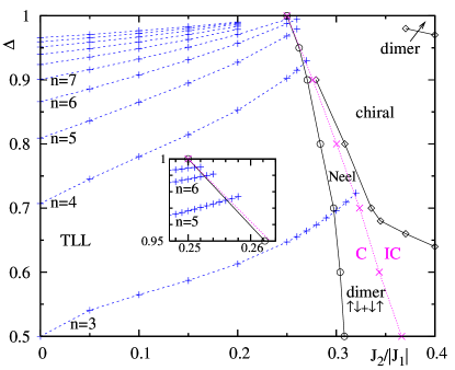
Figure 3: (color online) Phase diagram of the model (1). The level spectroscopy has been performed for $L=24$. We have observed that finite-size effects are quite small and can be neglected. The inset shows a zoom around the highly-degenerate point $(J_{2}/|J_{1}|,\Delta)=(1/4,1)$.

III Phase diagram

The phase diagram is determined by the level spectroscopy and the iTEBD analysis as presented in Fig. 3. The blue “+” symbols show Gaussian fixed points determined from the condition $E_{\rm N}=E_{\rm D}$. The black open circles interpolated by lines show the transition points from the TLL phase to the Néel and dimer phases, which are determined by $E_{\rm S}=E_{\rm N}$ and $E_{\rm S}=E_{\rm D}$, respectively. This phase boundary between the TLL phase and the gapped ordered phases is smoothly connected to the ferromagnetic transition pointBursill95 $J_{2}/|J_{1}|=1/4$ in the isotropic case $\Delta=1$, at which the ground states are known to be highly degenerate.Hamada88 The Gaussian fixed lines with $\lambda=0$ start from the “special” points given in Eq. (7) at $J_{2}=0$, and are therefore labeled by $n=3,4,\dots$ for convenience. Some of them continue even after the cosine potential becomes relevant for $J_{2}/|J_{1}|>1/4$. From calculation of $L=24$ system, we have identified five lines (corresponding to $n=3,\ldots,7$) extending into the parameter region $J_{2}/|J_{1}|>1/4$ and $\Delta\lesssim 0.995$. Across these lines, there occur successive transitions between the Néel and dimer phases as the anisotropy parameter $\Delta$ is changed toward unity. However, for $0.995\lesssim\Delta\leq 1$, Lanczos diagonalization does not converge well, due to highly degenerate nature around $(J_{2}/|J_{1}|,\Delta)=(1/4,1)$. For this reason we have not been able to find the transition lines beyond $n=7$.

Inside the Néel and dimer phases, there is a Lifshitz line (pink “$\times$” symbols), where the short-range spin correlation in the $xy$ plane changes its character from commensurate to incommensurate (indicated by C and IC in Fig. 3). This line was determined by observing the peak position of the equal-time spin structure factor calculated by iTEBD.FSO The level spectroscopy presented above is valid on the left side of this line. By further increasing $J_{2}/|J_{1}|$, the system enters the vector chiral ordered phase in which the vector product of neighboring spins, $\kappa_{j,j+1}^{z}:=\langle(\bm{S}_{j}\times\bm{S}_{j+1})^{z}\rangle$, is long-range ordered. The boundaries above and below the vector chiral phase (black diamond symbols) were determined with reasonable accuracy by observing the rapid increase of the order parameter $\kappa_{j,j+1}^{z}$ calculated by iTEBD.FSO For $0.9\lesssim\Delta<1$ and $0.25<J_{2}/|J_{1}|\lesssim 0.35$, we have not been able to locate the transition lines accurately because of a relatively poor convergence of iTEBD around the highly degenerate point $(J_{2}/|J_{1}|,\Delta)=(1/4,1)$. However, we expect that both the lines should continue to the point $(J_{2}/|J_{1}|,\Delta)=(1/4,1)$. The vector chiral phase is smoothly connected to that found in the frustrated ferromagnetic chain in a low magnetic field.Hikihara08 ; Sudan09 ; Heidrich09 Similar vector chiral phases have also been found previously in the antiferromagnetic $J_{1}$-$J_{2}$ model with easy-plane anisotropyNersesyan98 ; Hikihara01 or in a magnetic field.Kolezhuk05 ; McCulloch08 ; Okunishi08 ; Hikihara10

The nature of the dimer phase at $\Delta\lesssim 0.7$ is easy to understand, as this phase extends to the XY point $\Delta=0$, where the sign of $J_{1}$ can be reversed by performing the $\pi$ rotations around the $z$ axis of the spins on every second sites. From the fact that the ground state at the Majumdar-Ghosh point $J_{2}=J_{1}/2>0$ and $\Delta=0$ (and more generally for all $\Delta>-1/2$)Majumdar69 is given exactly by the product of singlet dimers $(|\!\uparrow\downarrow\rangle-|\!\downarrow\uparrow\rangle)/\sqrt{2}$, one finds, through the above $\pi$-rotation transformation, that the ground states at $J_{2}=-J_{1}/2>0$ and $\Delta=0$ are given by the dimer states whose dimer unit is now replaced by the triplet state $(|\!\uparrow\downarrow\rangle+|\!\downarrow\uparrow\rangle)/\sqrt{2}$.Chubukov91 We expect that such a “triplet” dimer nature should survive away from the XY point and define the order parameter of the dimer phase. The nature of the Néel phase in $0.7\lesssim\Delta\lesssim 0.9$ is more elusive and will be discussed in detail in the next section.

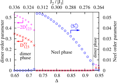
Figure 4: (color online) The dimer order parameters $D_{123}^{xy}$ and $-2D_{123}^{z}$ (left axis) and the local magnetization $\langle S_{1}^{z}\rangle$ (right axis), along the line connecting $(J_{2}/|J_{1}|,\Delta)=(0.336,0.65)$ and $(0.264,0.95)$, which approximately traces the Lifshitz line. The order parameters take on relatively large values along this line. The calculation was done by the iTEBD with the Schmidt rank $\chi=300$. The vertical lines indicate the phase boundaries determined by the level spectroscopy.

So far our argument for the emergence of the Néel and dimer phases has been based on the effective SG theory. To confirm their existence in an independent and unbiased way, we have calculated the order parameters of these phases using the iTEBD algorithm,Vidal07 which can address physical quantities in the thermodynamic limit directly through the use of the matrix product representation of (ground) states. When this algorithm is performed in an ordered phase, a variational state finally converges to a symmetry-broken state with a finite spontaneous order parameter (if it is allowed by the periodicity of the matrix product state). Hence, the Néel phase is detected by a local magnetization $\langle S_{1}^{z}\rangle$, and the dimer phase by dimer order parameters:

$$D_{123}^{xy} = (S_{1}^{x}S_{2}^{x}+S_{1}^{y}S_{2}^{y})-(S_{2}^{x}S_{3}^{x}+S_{2}^{y}S_{3}^{y}),$$ (16)

$$D_{123}^{z} = S_{1}^{z}S_{2}^{z}-S_{2}^{z}S_{3}^{z}.$$ (17)

These order parameters show alternating signs along the spin chain. We choose the site labellings in such a way that $\langle S_{1}^{z}\rangle>0$ and $D_{123}^{z}<0$. We calculated these order parameters for the parameter points $(J_{2}/|J_{1}|,\Delta)$ varying approximately along the Lifshitz line; see Fig. 4. In this figure we observe two transitions between the dimer and Néel phases, in agreement with the level spectroscopy analysis. In the dimer phases, $D_{123}^{xy}$ and $D_{123}^{z}$ show opposite signs in accord with the “triplet” nature of the dimers. [Notice that $D_{123}^{xy}=-2D_{123}^{z}=1/2$ in the exact “triplet” dimer state at $(J_{2}/|J_{1}|,\Delta)=(1/2,0)$.]

The sudden changes of the order parameters in Fig. 4 seem to indicate first-order nature of the transitions between Néel and dimer phases for this parameter regime. On the contrary, a continuous transition of Gaussian type is expected in the SG model (Fig. 1). This discrepancy may be reconciled by considering the effect of a higher-frequency cosine potential $\cos(8\sqrt{\pi}\phi)$, which was ignored in the SG theory but is allowed by symmetry, and can become relevant deep inside the ordered phases. With a negative coefficient, the potential $\cos(8\sqrt{\pi}\phi)$ has four minima corresponding to the Néel and dimer orderings with doubly-degenerate ground states each. Different signs of $\lambda$ select different types of orderings, and thus the first-order transition at $\lambda=0$ separates the two phases.

We finally note that, in the small region near the upper right corner of Fig. 3, a weak dimerization with the same sign in $D_{123}^{xy}$ and $D_{123}^{z}$ was observed.FSO In particular, $D_{123}^{xy}=2D_{123}^{z}$ in the isotropic case $\Delta=1$. This result indicates that this region is characterized as a dimer ordered phase having a distinct nature from the “triplet” dimer phase in $\Delta\lesssim 0.7$.

IV Nature of the Néel phase

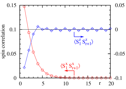
Figure 5: (color online) Spin correlation functions $\langle S^{x}_{1}S^{x}_{r+1}\rangle$ (left axis) and $\langle S^{z}_{1}S^{z}_{r+1}\rangle$ (right axis) for $J_{2}/|J_{1}|=0.31$ and $\Delta=0.74$, where the Néel order parameter is relatively large: $\langle S^{z}_{1}\rangle=-\langle S^{z}_{2}\rangle=0.04432$.

The appearance of the Néel phase is a natural consequence of the SG theory (3) with $\lambda>0$, but is quite counterintuitive in the presence of the easy-plane nearest-neighbor ferromagnetic coupling. In Fig. 4, the Néel order parameter is one order of magnitude smaller than the value $\langle S_{1}^{z}\rangle=1/2$ of the pure Néel state $|\!\uparrow\downarrow\uparrow\downarrow\dots\rangle$, which indicates that the ground state is not well approximated by such a simple product state. Here we analyze the nature of this phase in detail using iTEBD with Schmidt rank $\chi=200$. We first analyze the spin correlations; see Fig. 5. We observe that the Néel character of the correlations appears only at a relatively long-distance scale $r\gtrsim 6$. At a short-distance scale, $\langle S^{x}_{1}S^{x}_{1+r}\rangle$ takes larger amplitudes than $\langle S^{z}_{1}S^{z}_{1+r}\rangle$, reflecting the easy-plane anisotropy. Furthermore, we note that $\langle S^{z}_{1}S^{z}_{3}\rangle$ takes relatively large negative value, which is unusual in a Néel phase.

Such unusual correlations in a short-distance scale can be understood in terms of trimer degrees of freedom. First, we consider a three-spin model shown in Fig. 6(a). In the isotropic case $\Delta=1$, the ground state is a quadruplet $|q_{\mu}\rangle$ (with $S^{z}_{\rm tot}=\mu=\pm\frac{1}{2},\pm\frac{3}{2}$) when $J_{2}/|J_{1}|<1/2$. Because of the reflection symmetry around the site $2$, the excited states are classified into symmetric and antisymmetric doublets, $\{|d_{\mu}\rangle\}$ and $\{|d_{\mu}^{\prime}\rangle\}$ (with $\mu=\pm\frac{1}{2})$. When the anisotropy $\Delta$ is introduced, $|q_{\pm\frac{1}{2}}\rangle$ and $|d_{\pm\frac{1}{2}}\rangle$ are mixed to form new eigenstates $|\tilde{q}_{\pm\frac{1}{2}}\rangle$ and $|\tilde{d}_{\pm\frac{1}{2}}\rangle$. The eigenstates are summarized as follows:

$$|q_{+\frac{3}{2}}\rangle=|\!\uparrow\uparrow\uparrow\rangle,$$ (18a)

$$|\tilde{q}_{+\frac{1}{2}}(\gamma)\rangle=\frac{1}{\sqrt{2+\gamma^{2}}}(|\!\uparrow\uparrow\downarrow\rangle+|\!\downarrow\uparrow\uparrow\rangle+\gamma|\!\uparrow\downarrow\uparrow\rangle),$$ (18b)

$$|\tilde{d}_{+\frac{1}{2}}(\gamma)\rangle=\frac{1}{\sqrt{4+2\gamma^{2}}}(\gamma|\!\uparrow\uparrow\downarrow\rangle+\gamma|\!\downarrow\uparrow\uparrow\rangle-2|\!\uparrow\downarrow\uparrow\rangle),$$ (18c)

$$|d^{\prime}_{+\frac{1}{2}}\rangle=\frac{1}{\sqrt{2}}(|\!\uparrow\uparrow\downarrow\rangle-|\!\downarrow\uparrow\uparrow\rangle),$$ (18d)

with $\gamma=\frac{1}{2}(\sqrt{\tilde{\Delta}^{2}+8}-\tilde{\Delta})$ and $\tilde{\Delta}=\Delta+(J_{2}/|J_{1}|)(\Delta-1)$. Other eigenstates with $\mu=-1/2$ or $-3/2$ are obtained by applying the spin reversal to the above. The eigenenergies are plotted in Fig. 7. Under the easy-plane anisotropy $\Delta<1$, the ground states are given by $|\tilde{q}_{\pm\frac{1}{2}}(\gamma)\rangle$ (with $\gamma>1$), in which $S_{j}^{x}$’s correlate ferromagnetically and $S_{j}^{z}$’s antiferromagnetically for any spin pair (if $\gamma<\sqrt{2}$). This property is in accord with the anomalous spin correlations in Fig. 5 for $r=1,2$. Note, however, that the local magnetization $\langle S_{j}^{z}\rangle$ is almost uniform in $|\tilde{q}_{\pm\frac{1}{2}}(\gamma)\rangle$ as shown in Fig. 6(a), and we do not observe Néel ordering pattern at this level.

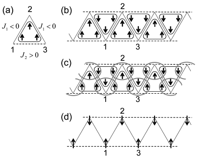
Figure 6: (a): Three-spin model. (b), (c), (d): Neel order from the trimer picture. The arrows show the $z$-component of the local magnetization.

Now we construct a Néel ordered state in a 1D chain as follows. (The procedure is analogous to the construction of the valence bond solid ground state in the Affleck-Kennedy-Lieb-Tasaki model,Affleck87 and more generally to the construction of a projected entangled-pair state.Verstraete04 ) The 1D model (1) can be viewed as the model on the zigzag ladder, where $J_{1}$ and $J_{2}$ give the inter- and intra-chain couplings respectively. We place a trimer state $|\tilde{q}_{+\frac{1}{2}}(\gamma)\rangle$ ($|\tilde{q}_{-\frac{1}{2}}(\gamma)\rangle$ resp.) on every up (down resp.) triangle in the zigzag ladder, as shown in Fig. 6(b). At this point, every site is shared by three neighboring trimers. To define the state in the original Hilbert space, we bind the three spins at every site together to form a single spin-$1/2$, as indicated by an ellipse in Fig. 6(c). This is done by a projection operator $|\!\uparrow\rangle\langle\psi_{+}|+|\!\downarrow\rangle\langle\psi_{-}|$, where $|\psi_{\pm}\rangle$ are defined for the three spins in an ellipse. We require that (i) $|\psi_{\pm}\rangle$ have the reflection symmetry about the central spin and that (ii) they have sufficient overlap with $|\!\!\uparrow\downarrow\uparrow\rangle$ and $|\!\!\downarrow\uparrow\downarrow\rangle$, which are expected to have large weights in the state before projection as can be seen in Fig. 6(c). The states satisfying (i) can be written in the same way as in Eq. (18a)-(18c). Considering also (ii), we set $|\psi_{\pm}\rangle=|\tilde{d}_{\pm\frac{1}{2}}(\gamma^{\prime})\rangle$ with $\gamma^{\prime}$ appropriately tuned. The obtained state after the projection has a Néel ordering pattern as shown in Fig. 6(d). We expect that this should give an approximate ansatz (with two variational parameters, $\gamma$ and $\gamma^{\prime}$) of the Néel ground state found in the present model.

Figure 7: Spectrum of the three-spin model in Fig. 6(a) for $J_{2}/|J_{1}|=0.31$. The eigenstates are given in Eqs. (18).

To support the trimer picture, we calculated the reduced density matrix $\rho_{123}$ for neighboring three spins $(1,2,3)$ from the ground state obtained by the iTEBD. It was done for the same parameter point as in Fig. 5. Because of the reflection symmetry about the site $2$, $\rho_{123}$ is diagonalized in the form

$$\begin{split}\rho_{123}=&\,|q_{+\frac{3}{2}}\rangle a_{+}\langle q_{+\frac{3}{2}}|+|\tilde{q}_{+\frac{1}{2}}(\gamma_{+})\rangle b_{+}\langle\tilde{q}_{+\frac{1}{2}}(\gamma_{+})|\\ &+|\tilde{d}_{+\frac{1}{2}}(\gamma_{+})\rangle c_{+}\langle\tilde{d}_{+\frac{1}{2}}(\gamma_{+})|+|d_{+\frac{1}{2}}^{\prime}\rangle e_{+}\langle d_{+\frac{1}{2}}^{\prime}|\\ &+(\text{``}+\text{''}\to\text{``}-\text{''}),\end{split}$$ (19)

where $\gamma_{+}=1.225$ and $\gamma_{-}=1.250$ are not far from $\gamma=1.122$ obtained in the three-spin problem. Large weights are found in $b_{+}=0.5803$, $b_{-}=0.2633$, $e_{-}=0.0999$ and $a_{-}=0.0472$, and the others are orders of magnitude smaller. We see that the trimer states $|\tilde{q}_{\pm\frac{1}{2}}(\gamma_{\pm})\rangle$ occupy about 84% of the total weight.

We also applied the systematic method for determining the order parameter proposed in Ref. FMO06, . In this method, we use the pair of symmetry-broken ground states $|\Psi_{1,2}\rangle$ – one is obtained directly by iTEBD and the other by applying the spin reversal to it. For a subregion $A$ of the system, we construct the reduced density matrices $\rho_{A}^{1,2}$ from these states, and measure the mutual distance:

$${\rm diff}(\rho_{A}^{1},\rho_{A}^{2})=\sum_{j}|\lambda_{j}|,$$ (20)

where $\lambda_{j}$’s are the eigenvalues of $\rho_{A}^{1}-\rho_{A}^{2}$. This measure takes a value from zero to two and shows to what extent the two states are distinguished in the concerned region. [See Refs. FMO06, ; Furukawa07, for details.] For one- and two-site regions, we obtain the same value ${\rm diff}=4\langle S^{z}_{1}\rangle=0.1773$. The three-site region $A=\{1,2,3\}$ gives a much larger value ${\rm diff}=0.9128$. These results indicate that, although the symmetry breaking can be detected through a single-spin operator as expected for a Néel phase, it is much more visible in terms of a three-spin operator. This also supports the trimer picture for the Néel state.

Finally, we note that a Néel ordering in the presence of easy-plane anisotropy has been found in an antiferromagnetic model with explicit trimerization.Okamoto02 This example also suggests that the formation of trimers can change the nature of the anisotropy of the system.

V Conclusions

We have analyzed the phase diagram of the spin-$\frac{1}{2}$ frustrated ferromagnetic chain (1), starting from the bosonization picture in the unfrustrated case $J_{2}=0$. A crucial observation is that the effective sine-Gordon theory shows a cascade of sign changes in the coupling of the cosine potential when changing the anisotropy $\Delta$. When the cosine potential is made relevant by the competing $J_{2}$ exchange interaction, it gives rise to alternate appearance of Néel and dimer orders. Although the Néel phase has a long-ranged staggered spin ordering pattern, we have argued that this ordering should rather be interpreted as the ordering of the trimer degrees of freedom.

The successive sign changes in the coupling of the cosine term in the effective theory of the FM $J_{1}$ XXZ chain is explicitly seen in the exact expression (5) obtained in Refs. Lukyanov98, ; Lukyanov03, . Our study has shown for the first time that it has a dramatic physical consequence, the alternation of the Néel and dimer ordered phases. It will be interesting to further examine the effect of the sign change in the presence of other types of perturbations.

Appendix A Finite-size spectra in the sine-Gordon theory

In this appendix, following CardyCardy86 and Bortz et al.,Bortz09 we present a simple derivation of the excitation energies (14) based on the perturbation theory from the Gaussian model. This is complementary to the derivation by NomuraNomura95 using the correlation functions.

In a finite-size system of length $L$, the effective Hamiltonian is given by

$$H= H_{\rm Gauss}+H_{\cos}$$

$$= \int_{0}^{L}dx\left\{\frac{v}{2}\left[K\left(\frac{d\theta}{dx}\right)^{2}+\frac{1}{K}\left(\frac{d\phi}{dx}\right)^{2}\right]\right.$$

$$\left.\qquad\qquad-\frac{v\lambda}{2\pi}\cos(\sqrt{16\pi}\phi)\right\},$$ (21)

where the lattice spacing is set to unity.

Let us start from the Gaussian part $H_{\rm Gauss}$. It is useful to rescale the fields as $\Phi\equiv\phi/\sqrt{K}$ and $\Theta\equiv\sqrt{K}\theta$ to simplify the Hamiltonian:

$$H_{\rm Gauss}=\int_{0}^{L}dx~{}\frac{v}{2}\left[\left(\frac{d\Theta}{dx}\right)^{2}+\left(\frac{d\Phi}{dx}\right)^{2}\right].$$ (22)

Assuming the periodic boundary condition, we perform the mode expansions of the bosonic fields:

$$\Phi(x)=\Phi_{0}+\widetilde{Q}\frac{x}{L}+\sum_{n\neq 0}\frac{e^{-|n|/2\Lambda}}{\sqrt{4\pi|n|}}\left(e^{ik_{n}x}a_{n}+e^{-ik_{n}x}a_{n}^{\dagger}\right),$$ (23)

$$\Theta(x)=\Theta_{0}+Q\frac{x}{L}$$

$$\hskip 28.45274pt+\sum_{n\neq 0}\frac{e^{-|n|/2\Lambda}}{\sqrt{4\pi|n|}}{\rm sign}(n)\left(e^{ik_{n}x}a_{n}+e^{-ik_{n}x}a_{n}^{\dagger}\right),$$ (24)

with $k_{n}=2\pi n/L$. Here, $a_{n}$ with $n>0$ ($n<0$) represents a right (left) moving mode. We have introduced an ultraviolet cutoff $\Lambda$, which will be determined later. The operators in the expansions obey the commutation relations

$$\begin{split}&[\Phi_{0},\Theta_{0}]=-i,\quad[\widetilde{Q},\Theta_{0}]=i,\quad[Q,\Phi_{0}]=i,\\ &[a_{n},a_{m}^{\dagger}]=\delta_{nm}.\end{split}$$ (25)

Using the mode expansions, the Hamiltonian is diagonalized as

$$H_{\rm Gauss}=\frac{2\pi v}{L}\left[\frac{1}{4\pi}(\widetilde{Q}^{2}+Q^{2})+\sum_{n\neq 0}|n|a_{n}^{\dagger}a_{n}\right],$$ (26)

where $\Lambda$ is taken to infinity. The ground state $|0\rangle$ is defined by $a_{n}|0\rangle=\widetilde{Q}|0\rangle=Q|0\rangle=0$ and its energy is set to zero. The compactification radii $R$ and $\tilde{R}$ for $\Phi$ and $\Theta$ are given by

$$2K=\frac{1}{2\pi R^{2}}=2\pi\tilde{R}^{2}.$$ (27)

Then $\widetilde{Q}$ and $Q$ are quantized as

$$\widetilde{Q}=S^{z}/\tilde{R},\quad Q=m/R,\quad\text{with}~{}S^{z},m\in\mathbb{Z}.$$ (28)

Here, the integer $S^{z}$ coincides with the total magnetization. The entire spectrum is then given by

$$\begin{split}&\Delta E_{0}(S^{z},m,\{m_{n}\})\\ &=\frac{2\pi v}{L}\left[\frac{1}{4\pi}\left(\frac{(S^{z})^{2}}{\tilde{R}^{2}}+\frac{m^{2}}{R^{2}}\right)+\sum_{n\neq 0}|n|m_{n}\right]\end{split}$$ (29)

with $m_{n}\geq 0$ integer, and the corresponding eigenstates are

$$\begin{split}|S^{z},m,\{m_{n}\}\rangle=e^{iS^{z}\Theta_{0}/\tilde{R}+im\Phi_{0}/R}\prod_{n\neq 0}(a_{n}^{\dagger})^{m_{n}}|0\rangle.\end{split}$$ (30)

The excitation $\Delta E_{\rm S}$ is associated with $e^{\pm i\Theta_{0}/\tilde{R}}$ and is thus given by

$$\Delta E_{\rm S}=\Delta E(\pm 1,0,0)=\frac{2\pi v}{L}\frac{1}{4\pi\tilde{R}^{2}}=\frac{2\pi v}{L}\frac{1}{2+y},$$ (31)

with $y\equiv 4K-2$. This coincides with the expression (14a) when $|y|\ll 1$. On the other hand, $\Delta E_{\rm N/D}$ are associated with $\cos(\Phi_{0}/R)$ and $\sin(\Phi_{0}/R)$ respectively. In the Gaussian model, these energies are degenerate and are given by

$$\Delta E_{\rm N/D}=\Delta E(0,\pm 1,0)=\frac{2\pi v}{L}\frac{1}{4\pi R^{2}}=\frac{2\pi v}{L}K.\quad$$ (32)

So far, we have ignored the cutoff $\Lambda$. It is determined so that the two-point correlation function of vertex operators satisfies the simple normalization condition

$$\langle 0|e^{i\mu\Phi(x)}e^{-i\mu\Phi(x^{\prime})}|0\rangle=\frac{1}{|x-x^{\prime}|^{\mu^{2}/2\pi}}$$ (33)

for $|x-x^{\prime}|\ll L$. Using the expansion (23), the l.h.s. of Eq. (33) is evaluated as

$$\exp\left[-\mu^{2}\langle 0|\Phi(x)\Phi(x^{\prime})|0\rangle\right]$$

$$=\exp\!\left[-\mu^{2}\sum_{n\neq 0}\frac{e^{-|n|/\Lambda}}{4\pi|n|}\left(1-e^{2\pi i|n|(x-x^{\prime})/L}\right)\right]$$

$$=\left|\frac{1-e^{-\frac{1}{\Lambda}+i\frac{2\pi(x-x^{\prime})}{L}}}{1-e^{-\frac{1}{\Lambda}}}\right|^{-\mu^{2}/2\pi}$$

$$\approx\left(2\Lambda\sin\frac{\pi|x-x^{\prime}|}{L}\right)^{-\mu^{2}/2\pi}.$$ (34)

Hence, we set $\Lambda=L/2\pi$ to satisfy Eq. (33).

Now we introduce $H_{\cos}$ as a perturbation. It splits the degeneracy between $\Delta E(0,\pm 1,0)$. We calculate the matrix element:

$$\begin{split}C&:=\langle 0,-1,0|H_{\cos}|0,1,0\rangle\\ &=-\frac{v\lambda}{2\pi}\int_{0}^{L}dx\,\langle 0|e^{i\Phi_{0}/R}\cos\left(\frac{2\Phi(x)}{R}\right)e^{i\Phi_{0}/R}|0\rangle.\end{split}$$ (35)

Using the expansion (23), the integrand is evaluated as

$$\begin{split}&\langle 0|e^{i\Phi_{0}/R}\cos\left(\frac{2\Phi(x)}{R}\right)e^{i\Phi_{0}/R}|0\rangle\\ &=\frac{1}{2}\langle 0|e^{i\Phi_{0}/R}e^{-2i\Phi(x)/R}e^{i\Phi_{0}/R}|0\rangle\\ &=\frac{1}{2}\langle 0|\exp\!\left[-\frac{2i}{R}\sum_{n\neq 0}\frac{e^{-|n|/2\Lambda}}{\sqrt{4\pi|n|}}\left(e^{2\pi inx/L}a_{n}+\mathrm{H.c.}\right)\right]\!|0\rangle\\ &=\frac{1}{2}\exp\!\left(-\frac{1}{\pi R^{2}}\sum^{\infty}_{n=1}\frac{e^{-n/\Lambda}}{n}\right)=\frac{1}{2}\Lambda^{-4K}.\end{split}$$ (36)

In first-order perturbation theory the new eigenstates are given by the linear combinations

$$\frac{1}{\sqrt{2}}(|0,1,0\rangle\pm|0,-1,0\rangle),$$ (37)

and the corresponding eigenenergies are

$$\begin{split}\Delta E_{\rm N/D}=\frac{2\pi v}{L}K\pm C=\frac{2\pi v}{L}\left[\frac{1}{2}+\frac{y}{4}\mp\lambda\left(\frac{2\pi}{L}\right)^{y}\right].\end{split}$$ (38)

Equations (31) and (38) are non-perturbative in $y$ and perturbative in $\lambda$.

So far, we have used the bare coupling constants, $y$ and $\lambda$. Now we relate the above results to the running coupling constants, $y(l)$ and $y_{\phi}(l)$, focusing on the vicinity of the multicritical point $(y,y_{\phi})=(0,0)$. Both the cosine potential and the change in the Luttinger parameter $y$ are marginal perturbations at this point. In general, the excitation energy $\Delta E_{n}$ associated with an operator ${\cal O}_{n}$ is related to the inverse of the correlation length $\xi_{n}$ of the operator. Under a global scale transformation by a factor $e^{l}$, it scales as

$$\Delta E_{n}\propto\xi_{n}^{-1}(y,y_{\phi},L^{-1})=e^{-l}\xi_{n}^{-1}(y(l),y_{\phi}(l),L^{-1}e^{l}).$$ (39)

Setting $e^{l}=L/2\pi$, this is given by a universal function in terms of $y(l)$ and $y_{\phi}(l)$:

$$\Delta E_{n}=\frac{2\pi}{L}\Phi_{n}(y(l),y_{\phi}(l)).$$ (40)

Namely, $L\Delta E_{n}$ depends on $L$ only through $y(l)$ and $y_{\phi}(l)$.

We compare this with Eqs. (31) and (38). As shown in Fig. 1, for $y>|y_{\phi}|$, $y(l)$ finally converges to a constant. If the bare value of $y$ is sufficiently close to the final constant, the RG equations are solved as

$$y(l)=y,~{}~{}y_{\phi}(l)=y_{\phi}e^{-yl}.$$ (41)

Thus, under the correspondence $e^{l}=L/2\pi$, Eqs. (31) and (38) are expressed by Eqs. (14), which show a linear dependence on $y(l)$ and $y_{\phi}(l)$. Equation (40) implies that we can extend the range of validity of Eqs. (14) to all $|y(l)|,|y_{\phi}(l)|\ll 1$.

References

- (1) P. Lecheminant, in Frustrated spin systems, edited by H. T. Diep (World-Scientific, Singapore, 2005), Review chapter; arXiv:cond-mat/0306520.
- (2) M. Hase, H. Kuroe, K. Ozawa, O. Suzuki, H. Kitazawa, G. Kido, and T. Sekine, Phys. Rev. B 70, 104426 (2004).
- (3) T. Masuda, A. Zheludev, B. Roessli, A. Bush, M. Markina, and A. Vasiliev, Phys. Rev. B 72, 014405 (2005).
- (4) M. Enderle, C. Mukherjee, B. Fåk, R.K. Kremer, J.-M. Broto, H. Rosner, S.-L. Drechsler, J. Richter, J. Malek, A. Prokofiev, W. Assmus, P. Pujol, J.-L. Raggazzoni, H. Rakoto, M. Rheinstädter, and H.M. Rønnow, Europhys. Lett. 70, 237 (2005).
- (5) S.-L. Drechsler, O. Volkova, A. N. Vasiliev, N. Tristan, J. Richter, M. Schmitt, H. Rosner, J. Málek, R. Klingeler, A. A. Zvyagin, and B. Büchner Phys. Rev. Lett. 98, 077202 (2007).
- (6) A. V. Chubukov, Phys. Rev. B 44, 4693 (1991).
- (7) A. Kolezhuk and T. Vekua, Phys. Rev. B 72, 094424 (2005).
- (8) F. Heidrich-Meisner, A. Honecker, and T. Vekua, Phys. Rev. B 74, 020403 (R) (2006).
- (9) T. Vekua, A. Honecker, H.-J. Mikeska, F. Heidrich-Meisner, Phys. Rev. B 76, 174420 (2007).
- (10) L. Kecke, T. Momoi, and A. Furusaki, Phys. Rev. B 76, 060407 (R) (2007).
- (11) T. Hikihara, L. Kecke, T. Momoi, and A. Furusaki, Phys. Rev. B 78, 144404 (2008).
- (12) J. Sudan, A. Luscher, and A. M. Läuchli, Phys. Rev. B 80, 140402 (R) (2009).
- (13) M. Sato, T. Momoi, and A. Furusaki, Phys. Rev. B 79, 060406 (R) (2009).
- (14) F. Heidrich-Meisner, I.P. McCulloch, and A.K. Kolezhuk, Phys. Rev. B 80, 144417 (2009).
- (15) T. Tonegawa, I. Harada, and J. Igarashi, Prog. Theor. Phys. Suppl. 101, 513 (1990).
- (16) R. D. Somma and A. A. Aligia, Phys. Rev. B 64, 024410 (2001).
- (17) S. Furukawa, M. Sato, Y. Saiga, S. Onoda, J. Phys. Soc. Jpn. 77, 123712 (2008).
- (18) J. Sirker, Phys. Rev. B 81, 014419 (2010).
- (19) C.K. Majumdar and D.K. Ghosh, J. Math. Phys. 10, 1399 (1969).
- (20) F.D.M. Haldane, Phys. Rev. Lett. 45, 1358 (1980).
- (21) F.D.M. Haldane, Phys. Rev. B 25, 4925 (1982).
- (22) K. Okamoto and K. Nomura, Phys. Lett. A 169, 433 (1992).
- (23) K. Nomura and K. Okamoto, J. Phys. A 27, 5773 (1994).
- (24) S.R. White and I. Affleck, Phys. Rev. B 54, 9862 (1996)
- (25) A.A. Nersesyan, A.O. Gogolin, and F.H.L. Eßler, Phys. Rev. Lett. 81, 910 (1998).
- (26) T. Hikihara, M. Kaburagi, and H. Kawamura, Phys. Rev. B 63, 174430 (2001).
- (27) S. Lukyanov, Nucl. Phys. B 522, 533 (1998).
- (28) S. Lukyanov and V. Terras, Nucl. Phys. B 654, 323 (2003).
- (29) K. Nomura, J. Phys. A 28, 5451 (1995).
- (30) G. Vidal, Phys. Rev. Lett. 98, 070201 (2007).
- (31) S. Furukawa, M. Sato, and S. Onoda, arXiv:1003.3940 (unpublished); for a preliminary report, see S. Furukawa, M. Sato, Y. Saiga, and S. Onoda, an invited paper in 2008 activity report of Supercomputer Center at the Institute for Solid State Physics (URL: http://www.issp.u-tokyo.ac.jp/supercom/highlights/highlight/).
- (32) T. Giamarchi, Quantum Physics in One Dimension (Oxford University Press, New York, 2004).
- (33) A. O. Gogolin, A. A. Nersesyan, and A. M. Tsvelik, Bosonization and Strongly Correlated Systems (Cambridge University Press, Cambridge, England, 1998).
- (34) See also A. Furusaki and T. Hikihara, Phys. Rev. B 69, 094429 (2004); 70, 189902(E) (2004).
- (35) Note that is negative in the present paper while it is positive in Refs. Giamarchi04, ; Gogolin98, and other standard references. The sign of can be changed under the -rotations of spins around the axis on every second sites. The uniform and staggered parts in Eq. (9) are interchanged under this transformation.
- (36) S. Lukyanov and A. Zamolodchikov, Nucl. Phys. B 493, 571 (1997).
- (37) S. Lukyanov, Phys. Rev. B 59, 11163 (1999).
- (38) T. Hikihara and A. Furusaki, Phys. Rev. B 58, R583 (1998).
- (39) T. Deguchi, K. Fabricius, B.M. McCoy, J. Stat. Phys. 102, 701 (2001).
- (40) M. Bortz, M. Karbach, I. Schneider, and S. Eggert, Phys. Rev. B 79, 245414 (2009).
- (41) J.M. Kosterlitz and D.J. Thouless, J. Phys. C 6, 1181 (1973); J.M. Kosterlitz, J. Phys. C 7, 1046 (1974).
- (42) R. Bursill, G.A. Gehring, D.J.J. Farnell, J.B. Parkinson, T. Xiang, and C. Zeng, J. Phys.: Condens. Matter 7, 8605 (1995).
- (43) T. Hamada, J. Kane, S. Nakagawa, and Y. Natsume, J. Phys. Soc. Jpn. 57, 1891 (1988).
- (44) I.P. McCulloch, R. Kube, M. Kurz, A. Kleine, U. Schollwöck and A.K. Kolezhuk, Phys. Rev. B 77, 094404 (2008).
- (45) K. Okunishi, J. Phys. Soc. Jpn. 77, 114004 (2008).
- (46) T. Hikihara, T. Momoi, A. Furusaki, and H. Kawamura, unpublished
- (47) I. Affleck, T. Kennedy, E.H. Lieb, and H. Tasaki, Phys. Rev. Lett. 59, 799 (1987).
- (48) F. Verstraete and J.I. Cirac, cond-mat/0407066.
- (49) S. Furukawa, G. Misguich, and M. Oshikawa, Phys. Rev. Lett. 96, 047211 (2006).
- (50) S. Furukawa, Ph. D Thesis, Tokyo Institute of Technology, 2007 (URL: http://tdl.libra.titech.ac.jp/cgi-bin/z3950/gakui-detail-disp.cgi?REG-NO=117193284).
- (51) K. Okamoto and Y. Ichikawa, J. Phys. Chem. Solids 63, 1575 (2002).
- (52) J.L. Cardy, Nucl. Phys. B270, 186 (1986); J. Phys. A: Math. Gen. 19, L1093 (1986).