The Spitzer Survey of the Small Magellanic Cloud (S³MC): Insights into the Life-Cycle of Polycyclic Aromatic Hydrocarbons

Abstract

We present the results of modeling dust spectral energy distributions (SEDs) across the Small Magellanic Cloud (SMC) with the aim of mapping the distribution of polycyclic aromatic hydrocarbons (PAHs) in a low-metallicity environment. Using Spitzer Survey of the SMC (S³MC) photometry from 3.6 to 160 µm over the main star-forming regions of the Wing and Bar of the SMC along with spectral mapping observations from 5 to 38 µm from the Spitzer Spectroscopic Survey of the Small Magellanic Cloud (S⁴MC) in selected regions, we model the dust spectral energy distribution and emission spectrum to determine the fraction of dust in PAHs across the SMC. We use the regions of overlaping photometry and spectroscopy to test the reliability of the PAH fraction as determined from SED fits alone. The PAH fraction in the SMC is low compared to the Milky Way and variable–with relatively high fractions ($q_{\rm PAH}$$\sim 1-2$%) in molecular clouds and low fractions in the diffuse ISM (average $\langle$$q_{\rm PAH}$$\rangle=0.6$%). We use the map of PAH fraction across the SMC to test a number of ideas regarding the production, destruction and processing of PAHs in the ISM. We find weak or no correlation between the PAH fraction and the distribution of carbon AGB stars, the location of supergiant H I shells and young supernova remnants, and the turbulent Mach number. We find that the PAH fraction is correlated with CO intensity, peaks in the dust surface density and the molecular gas surface density as determined from 160 µm emission. The PAH fraction is high in regions of active star-formation, as predicted by its correlation with molecular gas, but is supressed in H II regions. Because the PAH fraction in the diffuse ISM is generally very low–in accordance with previous work on modeling the integrated SED of the SMC–and the PAH fraction is relatively high in molecular regions, we suggest that PAHs are destroyed in the diffuse ISM of the SMC and/or PAHs are forming in molecular clouds. We discuss the implications of these observations for our understanding of the PAH life cycle, particularly in low-metallicity and/or primordial galaxies.

1. Introduction

Polycyclic Aromatic Hydrocarbons (PAHs) are thought to be the carrier of the ubiquitously observed mid-IR emission bands (Allamandola et al. 1989, among others). The bands are the result of vibrational de-excitation of the PAH skeleton through bending and stretching modes of C-H and C-C bonds after the absorption of a UV photon. The emission in these bands can be very bright and can comprise a significant fraction, up to 10$-$20% (Smith et al. 2007), of the total infrared emission from a galaxy. For this reason, PAH emission has been suggested to be a useful tracer of the star-formation rate, even out to high redshifts (Calzetti et al. 2007). Making use of PAHs as a tracer, however, requires understanding how the abundance and emission from PAHs depends on galaxy properties such as metallicity and star-formation history.

PAHs also play a number of important roles in the interstellar medium (ISM). In particular, these small dust grains can dominate photoelectric heating rates (Bakes & Tielens 1994). In dense clouds, PAHs can alter chemical reaction networks by providing a neutralization route for ionized species (Bakes & Tielens 1998; Weingartner & Draine 2001) and contribute large amounts of surface area for chemical reactions that occur on grain surfaces. PAHs are a crucial component of interstellar dust so we would like to understand the processes that govern their abundance and physical state.

The life-cycle of PAHs, however, is not yet well understood. PAHs are thought to form in the carbon-rich atmospheres of some evolved stars (Latter 1991; Cherchneff et al. 1992). Emission from PAHs has been observed from carbon-rich asymptotic giant branch stars (Sloan et al. 2007) and more frequently in carbon-rich post-AGB stars where the radiation field is more effective at exciting the mid-IR bands (Buss et al. 1993). A “stardust” origin (i.e. formation in the atmospheres of evolved stars) for the majority of PAH material is controversial, however, because it has yet to be demonstrated that PAHs can be produced in AGB stars faster than they are destroyed in the ISM (for a recent review, see Draine 2009), i.e. the timescale for destruction of dust by SNe shocks is shorter than the timescale over which the ISM is enriched with dust from AGB stars (for example, Jones et al. 1994). In addition to destruction by supernova shocks, PAH material may be destroyed by UV fields, a process that can dominate near a hot star or in the ISM of low metallicity and/or primordial galaxies. If PAHs are mostly not “stardust”, they must have formed in the ISM itself, by some mechanism which is not yet characterized. A variety of mechanisms have been suggested (Tielens et al. 1987; Puget & Leger 1989; Herbst 1991; Greenberg et al. 2000) however there is little observational support for any one model as of yet.

In recent years, observations with ISO and Spitzer have allowed us to study the abundance and physical state of PAHs in a variety of ISM conditions beyond those we observe in the Milky Way. One of the most striking results is the abrupt change in the fraction of dust in PAHs as a function of metallicity. A deficit of PAH emission from low metallicity galaxies has been widely observed (Madden 2000; Engelbracht et al. 2005; Madden et al. 2006; Wu et al. 2006; Jackson et al. 2006; Engelbracht et al. 2008). Engelbracht et al. (2005) found that the ratio of the 8 to 24 µm surface brightness undergoes a transition from a SED with typical PAH emission to an SED essentially devoid of PAH emission at a metallicity of 12 + log(O/H) $\sim 8$. The weakness of PAH emission in low-metallicity galaxies has been confirmed spectroscopically (Wu et al. 2006; Engelbracht et al. 2008). Using the SINGS galaxy sample Draine et al. (2007) modeled the integrated SEDs and determined that the deficit of PAH emission corresponds to a decrease in the PAH fraction rather than a change in excitation of the PAHs. They found that $q_{\rm PAH}$ (defined as the fraction of the total dust mass that is contributed by PAHs containing less than $10^{3}$ carbon atoms) changes from a median of $\sim 4$% (comparable to the Milky Way PAH fraction of 4.6%; Li & Draine 2001) in galaxies with 12 + log(O/H) $>8.1$ to a median of $\sim 1$% in more metal poor galaxies. Muñoz-Mateos et al. (2009) have investigated the radial variation of $q_{\rm PAH}$ and metallicity in the SINGS sample and find results consistent with Draine et al. (2007).

There have been a number of suggestions as to what in the PAH life-cycle changes at low metallicity leading to the observed deficiency. Galliano et al. (2008) suggested that the delay between enrichment of the ISM by supernova-produced dust relative to that from AGB stars could lead to a lower PAH fraction at low metallicity. This model relies on the assumption that supernovae contribute a significant amount of dust to the ISM, an assumption which is controversial (Moseley et al. 1989; Dunne et al. 2003; Krause et al. 2004; Sugerman et al. 2006; Meikle et al. 2007; Draine 2009), as well as long timescales for dust production in carbon-rich AGB stars, which may be shorter than previously thought (Sloan et al. 2009). Fundamentally, the Galliano et al. (2008) model assumes a “stardust” origin for PAHs, which may not be the case. Other models explaining the low metallicity deficiency rely on enhanced destruction of PAHs. This can be accomplished through more efficient destruction via supernova shocks (O’Halloran et al. 2006) or via the harder and more intense UV fields in these galaxies (e.g. Madden et al. 2006; Gordon et al. 2008).

In order to investigate the PAH life cycle at low metallicity, we performed two surveys of the Small Magellanic Cloud (SMC) with the Spitzer Space Telescope. The SMC is a nearby dwarf irregular galaxy that is currently interacting with the MW and the Large Magellanic Cloud. Its proximity (61 kpc; Hilditch et al. 2005), low metallicity (12 + log(O/H) $\sim 8$, $Z\sim 0.2Z_{\odot}$; Kurt & Dufour 1998) and tidally disrupted ISM make it an ideal location in which to study the life cycle of PAHs in an environment very different from the Milky Way. The SMC has a low dust-to-gas ratio, $\sim 10$ times smaller than in the Milky Way (Bot et al. 2004; Leroy et al. 2007), leading to more pervasive UV fields. Because of its proximity we can observe the ISM at high spatial resolution and sensitivity in order to characterize the processes driving the PAH fraction.

The PAH fraction in the SMC has been controversial. Li & Draine (2002), using IRAS and COBE data, found that the PAHs in the SMC Bar contained only 0.4% of the interstellar carbon, corresponding to $q_{\rm PAH}$$\approx$ 0.2%, whereas Bot et al. (2004) concluded that PAHs accounted for 4.8% of the total dust mass in the diffuse ISM of the SMC, similar to the Milky Way. In the following, we present results on the fraction of PAHs in the SMC using observations from the Spitzer Survey of the Small Magellanic Cloud (S³MC). We use spectroscopy in the regions covered by the Spitzer Spectroscopic Survey of the Small Magellanic Cloud (S⁴MC) to verify that our models for the photometry are correctly gauging the PAH fraction. We defer a detailed analysis of the spectroscopy to an upcoming paper (Sandstrom et al. 2010, in prep) In Section 2 we describe the observations and data reduction, particularly focusing on the foreground subtraction and cross-calibration of the IRAC, MIPS and IRS observations. In Section 3 we describe the SED fitting procedure using the models of Draine & Li (2007) and the modifications necessary to incorporate the S⁴MC spectroscopy into the fit. In Sections 4 and 5 we present the results of the SED modeling and discuss their implications for our understanding of the PAH life cycle both in low metallicity galaxies and in the Milky Way.

2. Observations and Data Reduction

2.1. Spitzer Survey of the Small Magellanic Cloud (S³MC) Observations

We mapped the main star-forming areas of the Bar and Wing of the SMC using the IRAC and MIPS instruments as part of the S³MC project (GO 3316). A more comprehensive description of the observations and data reduction can be found in Bolatto et al. (2007) and Leroy et al. (2007). The region where the coverage of the IRAC and MIPS observations overlap is shown in Figure 1 overlayed on the 24 µm image. The mosaics were constructed using the MOPEX software provided by the SSC. The IRAC and MIPS mosaics were corrected for a number of artifacts as described in Bolatto et al. (2007). The most important of these for the purposes of this work is the large additive gradients at IRAC wavelengths (primarily 5.8 and 8.0 µm) caused by varying offsets in the detectors and the mosaicing algorithm implemented in MOPEX. We will discuss these gradients further in Section 2.3 since they become important for determining the foregrounds present in our maps.

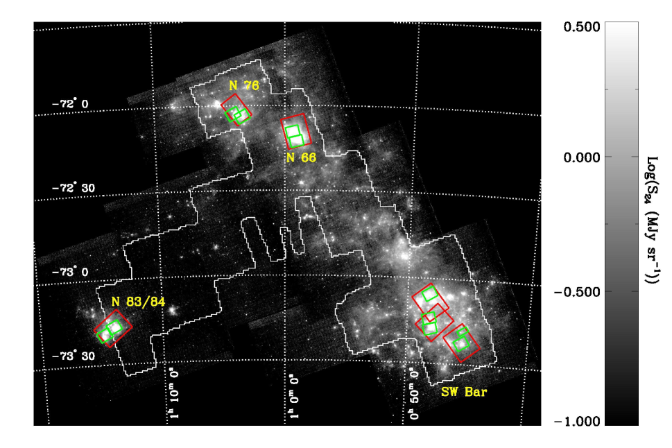
Figure 1.— The coverage of the S³MC and S⁴MC surveys overlayed on the MIPS 24 µm map. The color scale is logarithmic, with the stretch illustrated in the colorbar. The red boxes show the coverage of the LL1 order maps (the LL2 maps are shifted by $\sim 3\arcmin$) and the green boxes show the coverage of the SL1 order maps (the SL2 maps are shifted by $\sim 1\arcmin$). We also identify the various regions of the galaxy by the names we will refer to in the remainder of this paper.

Since the initial processing of the MIPS mosaics, the calibration factors recommended by the SSC have been revised. We correct the mosaics to use the recommended factors of 0.0454, 702 and 41.7 MJy sr^-1 per instrumental data unit, which are 3%, 11% and 0.7% different from the earlier values used by Bolatto et al. (2007) and Leroy et al. (2007). In addition, the 70 µm observations suffer from non-linearities at high surface brightness as noted by Dale et al. (2007). Although relatively few pixels in our map are affected by the correction, these regions in particular are most likely to overlap with our spectroscopic observations. We use the most recent non-linearity correction described in Gordon et al. (2010), in prep. No calibration correction for extended emission is necessary for the MIPS mosaics (Cohen 2009). The 1$\sigma$ sensitivities of the observations are listed in Table 1. The noise level at 70 µm is higher than the predicted detector noise due to pattern noise, visible as striping in the map (for further discussion of 70 µm noise properties, see Bolatto et al. 2007). Aside from the non-linearity corrections, we use the MIPS calibration factors listed on the SSC website, but we note that Leroy et al. (2007) found an offset between the MIPS 160 µm and the DIRBE 140 µm photometry of the SMC which may be the results of a calibration difference. They adjusted the calibration by a factor of 1.25 to match DIRBE. We do not apply this correction, and we briefly discuss the implications of that choice in Section 3.2.

Table 1S³MC Observation Details

Band	Map Noise Level	Cal. Uncertainty	Resolution
	(MJy sr-1)	(%)	(″)
3.6	0.015	10	1.66
4.5	0.017	10	1.72
5.8	0.055	10	1.88
8.0	0.042	10	1.98
24	0.047	4	6.0
70	0.664	7	18
160	0.695	12	40

Note. — The noise levels for the IRAC maps shown here have not been multiplied by the extended source calibration.

Because the calibration of the IRAC bands is based on stellar point sources and we are dealing with extended objects, we also apply the extended source calibration factors of 0.955, 0.937, 0.772 and 0.737 to the 3.6, 4.5, 5.8 and 8.0 bands as recommended by Reach et al. (2005). Recent work by Cohen et al. (2007) verified the 36% correction at 8.0 µm. The correction factors depend on the structure of the emission for each region of the map, which ranges from diffuse to point-like. Thus, applying on uniform correction factor across the entire map introduces some systematic uncertainty in our IRAC flux densities. To account for these uncertainties we assume a 10% calibration uncertainty for the IRAC bands. The details of the calibration are discussed further in an Appendix and the convolution and alignment to a common resolution will be discussed in Section 2.4.2.

2.2. Spitzer Spectroscopic Survey of the Small Magellanic Cloud (S⁴MC)

In order to directly probe the physical state of PAHs in the SMC, we performed spectral mapping of six star-forming regions using the low spectral resolution orders of IRS on Spitzer (GO 30491). These observations are primarily intended to investigate spectral variations in the PAH emission, to be described in Sandstrom et al. (2010), in prep. The coverage of the maps are shown overlayed on the MIPS 24 µm image from our S³MC observations in Figure 1.

The spectral coverage of the low-resolution orders of IRS extends from 5.2 to 38.0 µm, covering the major PAH emission bands in the mid-infrared except the 3.3 µm feature. The maps are fully sampled by stepping perpendicular to the slit one-half slit width between each slit position (1.85″and 5.08″, for SL and LL respectively). The LL maps are made of 98 pointings perpendcular to the slit and 7 pointings parallel for a coverage of $493\arcsec\times 474\arcsec$, except for the map of N 76 which covers 75 by 6 pointings and an area of $376\arcsec\times 395\arcsec$. The SL maps are made of 120 pointings perpendcular and 5 pointings parallel covering an area of $220\arcsec\times 208\arcsec$ in each map, except for the region around SMC B1 where we use 60 by 4 pointings covering an area of $109\arcsec\times 156\arcsec$.

The spectra were processed with either version 15.3.0 or 16.1.0 of the IRS Pipeline. The only difference of note between these versions is a change in the processing of radiation hits that does not affect the results we present. The details of the data reduction are discussed in Sandstrom et al. (2009). In brief, the maps were assembled using Cubism, wherein a “slit loss correction function” was applied, analogous to the extended source correction for the IRAC bands, to adjust the calibration from point sources to extended objects (Smith et al. 2007). Each mapping observation was followed or preceded by an observation of a designated “off” position at R.A. 1^h9^m40^s and Dec $-$73^∘31$\arcmin$30$\arcsec$. This position was seen to have minimal SMC emission in our MIPS observations. The “off” spectra, in addition to subtracting the zeroth-order foregrounds, help to mitigate the effects of rogue pixels. Additional bad pixel removal was done within Cubism. Beyond $\sim 35$ µm, there are increasing numbers of “hot” pixels which degrade the sensitivity of our spectra, we trim the LL orders to 35 µm to avoid issues with the long wavelength data.

Prior to further reduction steps we determine corrections to match the SL2 (5.2$-$7.6 µm), SL1 (7.5$-$14.5 µm), LL2 (14.5$-$20.75 µm) and LL1 (20.5$-$38.5 µm) orders in their overlap regions. For the SL2/SL1 and LL2/LL1 overlap, we find that the offsets are best explained by small additive effects, which may be due to a temporally and spatially varying dark current analogous to the “dark settle” effect seen in high-resolution IRS spectroscopy. Further discussion of these offsets will be presented in Sandstrom et al (2010), in prep. In brief, we apply correction factors determined by examining the unilluminated parts of the IRS detector, very similar to what is done in the “darksettle” software for LH available through the SSC. After applying these correction factors the orders generally match-up to within their respective errors. In regions of low surface brightness small residual effects have the appearance of a bump around 20 µm in the stitched spectra. These offsets only affect a small portion of the spectrum and do not measurably alter the results of the fit.

2.3. Foreground Subtraction

2.3.1 IRAC and MIPS Foreground Subtraction

In the mid- and far-infrared there are three major foreground/background contributions that contaminate our observations of the SMC: the zodiacal emission, Milky Way cirrus emission and the cosmic infrared background (CIB). In addition, for the IRAC mosaics there is a planar offset introduced by varying detector offsets and the mosaicing algorithm in MOPEX (see Bolatto et al. 2007, for more details). These need to be removed from the maps to isolate the emission from the SMC. In the following we will briefly discuss the foreground subtraction that has been carried out on our data and the major uncertainties in this process. The approach we use to subtract these foregrounds is motivated by the following limitations of our observations: (1) at longer wavelengths the mosaics do not extend to areas with no SMC emission, (2) the observations of neutral hydrogen which we use to subtract the Milky Way cirrus emission have a lower angular resolution than our Spitzer maps and (3) the residual mosaicing gradients in the 5.8, 8.0 and to a lesser degree 4.5 µm IRAC bands interfere with directly fitting and subtracting the zodiacal light.

Our foreground subtraction has three steps: (1) we determine the coefficients of a planar surface that describe the combination of zodiacal light and the residual mosaicing offsets, (2) we subtract this plane from each map at its native resolution, (3) we convolve the maps to the MIPS 160 µm resolution of 40″ and subtract the MW cirrus foreground and CIB. Throughout this procedure we fix the CIB level at 70 and 160 µm to be 0.23 and 1.28 MJy sr^-1 as determined from the Spitzer Observation Planning Tool (SPOT). We also assume a fixed proportionality between the infrared cirrus emission and the column density of MW H I (Boulanger et al. 1996), using coefficients derived from the model of Draine & Li (2007) for MW dust heated by the local interstellar radiation field. The Draine & Li (2007) model reproduces the DIRBE observations of the cirrus from Arendt et al. (1998) to within their quoted 20% uncertainties. We convolve the Draine & Li (2007) model emissivity spectrum with the IRAC and MIPS spectral response curves to obtain the coefficients, which are listed in Table 2. We use a map of Galactic hydrogen obtained by combining data from ATCA and Parkes (see Stanimirovic et al. 1999, for further information on the technique and the original observations) re-reduced and provided to us by E. Muller (private communication) to subtract the MW cirrus contribution.

Table 2Milky Way Foreground Coefficients

Band	Coefficient
	(MJy sr-1 (1021 H)-1)
3.6	0.018
4.5	0.006
5.8	0.070
8.0	0.215
24	0.162
70	2.669
160	11.097

The first step in our foreground subtraction is to determine the coefficients describing the planar contributions from the zodiacal light and the mosaicing offsets. Over the area of the SMC, the zodiacal light is well-described by a plane and the gradients introduced by the mosaicing algorithm also have a planar dependence (Bolatto et al. 2007). Unfortunately, there are no “off” locations where we could simply fit a plane to the foreground level, since no regions are totally free of SMC emission in the S³MC maps. At each position in the map the surface brightness is a combination of: SMC emission, MW cirrus emission, zodiacal light, mosaicing offsets and CIB. To isolate the planar component, we first extract photometry for a number of $200\arcsec\times 200\arcsec$ regions from the IRAC and MIPS maps. We choose the regions to be outside of star-forming areas, where the SMC emission is dominantly from dust heated by the general interstellar radiation field, where we can assume a proportionality between the dust emission and the SMC H I column. We choose the region size of $200\arcsec\times 200\arcsec$ to be larger than the 98″ beam of the H I observations and large enough to robustly determine the mean level in each box even when contaminated by point sources at the shorter wavelengths. We then subtract off the Milky Way cirrus contribution for those regions determined with the coefficients in Table 2 and the MW H I map, and, for the 70 and 160 µm maps, the CIB level. We call this MW cirrus and CIB subtracted value S_ν,resid. S_ν,resid is a combination of the zodiacal light, emission from the diffuse ISM of the SMC and whatever residual gradients there remain from the mosaicing for the IRAC maps. Next, using the SMC neutral H I observations of Stanimirovic et al. (1999), we perform a least-squares fit to the foreground values with the following function:

$$S_{\nu,{\rm resid}}=A(1+B\Delta_{\alpha}+C\Delta_{\delta})+D\times HI_{SMC}.$$ (1)

Here $A$, $B$ and $C$ are the coefficients describing a plane; $\Delta_{\alpha}$ and $\Delta_{\delta}$ are the gradients in Right Ascension and Declination across the SMC; $D$ is dust emission per H in the given waveband; and $S_{\nu,{\rm resid}}$ is the residual emission in each box after subtracting the MW foreground and CIB components. With this fit we determine the coefficients of the best fit planar foreground while excluding emission in the map coming from the SMC itself.

We take two additional steps to improve the determination of the planar foreground coefficients: (1) we use the 2MASS point source catalog to avoid regions of high stellar density in the IRAC bands so we do not subtract unresolved starlight, which can masquerade as a foreground, and (2) we fix the gradient of the zodiacal light ($B$ and $C$) at 70 and 160 µm  to the results of the fit at 24 µm. Since there are no mosiacing offsets for the MIPS bands, the zodiacal light is by far the dominant foreground at 24 µm and the zodiacal light should have the same spatial dependence at all of the MIPS wavelengths, fixing the zodiacal light gradient to what we measure at 24 µm is more effective than trying to fit for those coefficients at the longer wavelengths. The fixed pattern noise at 70 µm and the increasingly dominant SMC emission at 70 and 160 µm make the fitting procedure less robust compared to the 24 µm results.

The results of the fits are listed in Table 3. For the IRAC bands at 3.6 and 4.5 µm we do not detect any emission correlated with the SMC neutral hydrogen. At 4.5 µm, there is a quite significant residual gradient from the mosaicing procedure. At 3.6 µm the zodiacal foreground and its gradient are not detected at the sensitivity of the map. At both 3.6 and 4.5 unresolved starlight can play a role in the foreground determination, so we choose regions to avoid high stellar densities. In Table 3 we also list the standard deviations of the fit residuals to show the quality of the foreground determination for the mosaics. Finally, we subtract the planar fit listed in Table 3 from the mosaics at their full resolution.

Table 3Foreground Properties

Band	A	B	C	D	Std. Dev. of Fit
	(MJy sr-1)	(deg-1)		(MJy sr-1 (1020 H)-1)	(MJy sr-1)
3.6	$<$0.004	$\cdots$	$\cdots$	$\cdots$	0.011
4.5	$-$0.11	0.019	4.074	$\cdots$	0.014
5.8	4.99	$-$0.002	0.002	$9.14\times 10^{-4}$	0.023
8.0	3.69	0.0014	0.0014	$7.43\times 10^{-5}$	0.023
24	22.34	$-$0.0026	0.0010	$1.63\times 10^{-3}$	0.039
70	6.43	$-$0.0026	0.0010	$3.97\times 10^{-2}$	1.23
160	1.83	$-$0.0026	0.0010	$1.81\times 10^{-1}$	3.30

Note. — See Section 2.3.1 for a description of the coefficients.

Because it is at lower resolution (98″), we subtract the Milky Way foreground after convolving to the MIPS 160 µm resolution ($\sim 40$″). At the signal-to-noise ratio of the map, the Galactic H I in front of the SMC does not show any high contrast features, although there is a gradient ranging between 2 and 4$\times 10^{20}$ cm^-2 across the region. We note that the resolution difference between our mosaics and the H I observations means that there could be features with spatial scales less than 98″ that are not adequately subtracted from our maps. However, assuming a distance of 1 kpc for the H I foreground of the Galaxy, features left in our map would have to have spatial scales of $\sim 0.5$ pc. The typical foreground of Milky Way gas in this direction is $\sim 3\times 10^{20}$ cm^-3, an 0.5 pc cloud of cold neutral medium having a typical volume density of $\sim 40$ cm^-3 (Heiles & Troland 2003) would contribute a column of $6\times 10^{19}$ cm^-3, a factor of 5 less than the average foreground we see. Thus, we expect that inadequate subtraction of small scale structure will not greatly affect the quality of the foreground subtraction.

2.3.2 IRS Foreground Subtraction

The “off” observations for each spectral cube will remove foreground emission to first order. However, there are gradients between the “off” position and the cubes that are still present in the data. To remove the remaining foregrounds we add back to the spectra the difference between the “off” position and the map position at each wavelength calculated using the zodiacal light predictions from SPOT and the MW cirrus emission spectrum from Draine & Li (2007) multiplied by the MW H I column density at those locations.

2.4. Further Processing

2.4.1 Point Source Removal

The SED models which we use to determine the PAH fraction assume a stellar component in the Rayleigh-Jeans tail with $F_{\nu}\propto\nu^{2}$. In cases where this condition is not met, the presence of a stellar point source can corrupt the results of our fitting. In the vast majority of cases we see no problems relating to stellar point sources in the SMC, and thus we do not perform a comprehensive point source extraction on the observations. In addition, we are not able to remove any unresolved stellar contribution, so obtaining a map with the stellar component completely removed would require more detailed modeling. Instead, we mask out bright point sources which do not have a well behaved SED in the mid-IR. These sources typically fall into one of two categories: very bright stars which are saturated at one or more of the IRAC bands or stars with non-typical infrared SEDs, such as YSOs or carbon stars. We mask these objects out with a circular aperture which we fill in with the local background value.

2.4.2 Convolution and Alignment

The IRAC and MIPS mosaics are all convolved to match the resolution of the 160 µm observations using the kernels derived by Gordon et al. (2008) and available from the SSC. After convolution we regrid the maps to match the astrometry and pixel scale of the 160 µm mosaic.

For the IRS cubes, the convolution and alignment procedure involves a few additional steps. We convolve directly with the 160 µm PSF at each wavelength, which is much larger than the PSF of IRS even at its long wavelength end, so wavelength dependence of the PSF makes little difference to the final map. After convolution we align the cubes using the polygon clipping technique described in Sandstrom et al. (2009). Throughout this process, we appropriately propagate the uncertainty cubes produced by Cubism. Although the AORs are the largest possible size given the observation length limitations on Spitzer, the maps are only at most a few resolution elements across at 160 µm. Thus, we take some care to make sure that the spectra we use are only those where the PSF is not sampling regions outside the observed cube. For the following analysis we use only spectra where 90% of the area of the PSF or more is within the observed cube, which cuts down the number of viable spectra we can extract from the cubes to 63. The small number of resolution elements across the cube results in the introduction of scatter into the comparison between the MIPS and IRAC mosaics and the spectral maps. This is the result of information from outside the cube not being “convolved in”. This scatter represents a fundamental limitation of our observations. We estimate the magnitude of this scatter to be $\sim 10$% by comparing convolved and aligned IRAC 8.0 and MIPS 24 µm maps that have been cropped to the coverage of the spectral cubes to those that have not. For the SMC B1 cube we do not convolve or align the map because of the small number of resolution elements and the loss of signal due to the subsequent regridding to match at 160 µm. Instead we extract the spectrum for the whole SMC B1 spectral map and extract matching photometry from the IRAC and MIPS observations. After convolution and alignment we apply the previously mentioned correction factors to match the orders and stitch the cubes together in the overlaping spectral regions.

3. SED Model Fitting

We use the SED models of Draine & Li (2007) to determine the dust mass, radiation field properties and PAH fraction using our MIPS and IRAC mosaics in every independent pixel of the map where all of the MIPS and IRAC measurements are detected above $3\sigma$. We also perform simultaneous fits to photometry and spectroscopy in the regions covered by S⁴MC as described in Section 3.3. To distinguish between these two types of fits we introduce the following terminology: “photofit” refers to the best-fit model using only the photometry and “photospectrofit” refers to the best-fit model to the combined photometry and spectroscopy.

The model fit involves searching through a pre-made grid of models and finding the model which minimizes the following pseudo-$\chi^{2}$:

$$\chi^{2}=\sum_{b}\frac{\left(F_{\mathrm{obs},b}-\langle F_{\nu,\mathrm{model}}\rangle_{b}\right)^{2}}{\sigma^{2}_{\mathrm{obs},b}+\sigma^{2}_{\mathrm{model},b}}$$ (2)

Here $F_{\mathrm{obs},b}$ is the observed surface brightness in band $b$, $\langle F_{\nu,\mathrm{model}}\rangle_{b}$ is the model spectrum convolved with the spectral response curve of band $b$, $\sigma_{\mathrm{obs},b}$ is the uncertainty in the observed surface brightness and $\sigma_{\mathrm{model},b}$ is a factor which allows us to account for the systematics associated with the modeling. Following Draine et al. (2007) we use $\sigma_{\mathrm{model},b}=0.1F_{\nu,\mathrm{model},b}$.

The radiation field heating the dust is described by a power-law plus a delta function at the lowest radiation field:

$$\frac{dM_{D}}{dU}=(1-\gamma)M_{D}\delta(U-U_{min})+\gamma M_{D}\frac{(\alpha-1)}{U_{min}^{1-\alpha}-U_{max}^{1-\alpha}}U^{-\alpha}$$ (3)

Here $U$ is the radiation field in units of the interstellar radiation field in the Solar neighborhood from Mathis et al. (1983), $\gamma$ is the fraction of the dust heated by the minimum radiation field, $\alpha$ is the power-law index of the radiation field distribution and M_D is the dust mass surface density. This parametrization allows us to approximately account for both the dust heated by the general interstellar radiation field and the dust heated by nearby massive stars.

The adjustable parameters in the model are: the stellar luminosity per unit area ($\Omega_{*}$), the dust mass surface density (M_D), the PAH fraction ($q_{\rm PAH}$), the minimum and maximum radiation field (U_min and U_max), the fraction of dust heated by the minimum radiation field ($1-\gamma$) and the exponent of the radiation field power-law ($\alpha$). $\Omega_{*}$, M_D and $\gamma$ are continuous variables which normalize the grid of models to match the observations. The other variables are adjusted in discrete steps and can have the range of values listed in Table 4. Using the results of the fit we compute a number of useful parameters describing the outcome. These are $f_{PDR}$, the fraction of the total infrared power radiated by dust grains illuminated by radiation fields $U>10^{2}$, and $\bar{U}$, the average radiation field.

Table 4Draine & Li (2007) Model Parameters

Parameter	Range
$\Omega_{*}$	$>0$
MD	$>0$
$q_{\rm PAH}$	0.4$-$4.6%
Umin	0.6$-$30
Umax	$10^{3}-10^{7}$
$\gamma$	$>0$
$\alpha$	1.5$-$2.5

In the analysis we present here, we use the Draine & Li (2007) Milky Way (MW) dust model, so we take a moment to justify and explain this decision and its implications. In order to model the dust emission spectrum, it is necessary to choose a physical model for the dust which prescribes the abundances of different grains and their size distributions. At present, a dust grain size distribution model specific to the SMC including a variable PAH fraction and conforming to constraints on the dust mass and raw materials available has not been established, and producing such a model is complex and beyond the scope of this paper (it would require extending the model by Weingartner & Draine 2001). Note that because we are primarily interested in the PAH fraction, we must employ a model that includes a size distribution that extends into the PAH regime. In addition, we aim to compare our results with other studies of the PAH fraction (particularly that on the SINGS sample) which use the Milky Way dust model developed by Draine & Li (2007) and Draine et al. (2007).

There is evidence that the dust grain size distributions in the SMC and the Milky Way are different (Rodrigues et al. 1997; Weingartner & Draine 2001; Gordon et al. 2003), and that low metallicity galaxies in general may have an excess of small dust grains relative to the Milky Way. These differences, however, should not affect our measurements of the PAH fraction. Draine et al. (2007) found that the dust mass and PAH fraction from the best fit models for the galaxies in the SINGS sample that fell in the range of $q_{\rm PAH}$ covered by the LMC/SMC dust models were not significantly different if the Milky Way model was used instead, hence they employed Milky Way models. Given our desire to find the range of PAH fractions in the SMC and the benefit of being able to compare our results directly with those of Draine et al. (2007), we will fit MW dust models to the photometry.

We expect the choice of the MW dust models will introduce some systematic effects into the results of the model fitting. In particular, there is evidence that the SMC, like other low-metallicity galaxies, has a larger contribution from small grains compared to the Milky Way which results in “excess” emission at 24 and 70 µm (Gordon et al. 2003; Bot et al. 2004; Galliano et al. 2005; Bernard et al. 2008). The effect of such a population on our modeling will be to increase the best-fit radiation field in order to match the 24 and 70 µm brightness. Since we use a power-law distribution of radiation fields, and the equilibrium emission from large grains determines the minimum radiation field, the general effect is to decrease the power-law exponent and increase U_max, making a small fraction of the dust be heated by a more intense radiation field. Because the PAH emission is produced by single-photon heating, $q_{\rm PAH}$ is simply proportional to the ratio of the PAH emission in the 8 µm band to the total far-IR emission, which is robustly constrained by the 70 and 160 µm photometry. Hence, the derived $q_{\rm PAH}$ is relatively insensitive to variations in the U_min, U_max and $\alpha$, provided the observed total infrared luminosity is reproduced by the models. The regions with overlapping spectroscopy will provide a good test for this reasoning, since the $5-38$ µm continuum in conjunction with the 24, 70 and 160 µm SED provides more stringent constraints for the models. We will revisit this subject in Section 4.

3.1. The IRAC 4.5 µm Br$\alpha$ Contribution

The models we employ only calculate contributions to the IRAC and MIPS photometry from starlight, dust continuum and dust emission features. However, the emission spectrum from the ISM of the SMC is likely to contain a number of emission lines, particularly from H II regions, that contaminate the photometry. Most of these lines are very weak with respect to the dust continuum except in the case of the Brackett $\alpha$ hydrogen recombination line at 4.05 µm. Recent work by Smith & Hancock (2009) has shown that low-metallicity dwarf galaxies with recent star formation can have a Br$\alpha$ contribution that is a significant fraction of their integrated 4.5 µm flux. This problem is exacerbated within the H II regions themselves, where the 4.5 µm emission can be almost entirely from Br$\alpha$ (see for instance work on M 17 by Povich et al. 2007).

The SED models contain starlight continuum with a fixed 3.6 µm to 4.5 µm ratio. If there is excess 4.5 µm emission due to the hydrogen line, the starlight continuum will be too high, altering the ratio of stellar to non-stellar emission at 5.8 and 8.0 µm. To correct for the Br$\alpha$ emission, we use the Magellanic Cloud Emission Line Survey image of H$\alpha$ (kindly provided by C. Smith and F. Winkler; Smith & The MCELS Team 1999) along with the Case B factors at 10,000 K from Osterbrock & Ferland (2006) to convert H$\alpha$ to Br$\alpha$. This correction will underestimate the Br$\alpha$ emission where there is extinction, but since the intrinsic extinction in the SMC is low to begin with we expect this estimate of Br$\alpha$ to be adequate. This Br$\alpha$ correction is highest in H II regions, where we find Br$\alpha$ emission can account for 20-30% of the total 4.5 µm emission. Outside of H II regions, the correction is negligible.

3.2. Additional Systematic Uncertainties

Leroy et al. (2007) investigated the integrated far-IR SED of the SMC, using observations from IRAS, ISO, DIRBE and TOPHAT. They found that the MIPS 160 µm photometry is high by approximately 25% compared to the values predicted by interpolating from the DIRBE observations at 140 and 240 µm, a significant offset given how close in wavelength the DIRBE 140 and MIPS 160 bands are. More recent MIPS observations of the SMC obtained through the SAGE-SMC legacy survey (Gordon et al 2010, in prep.) agree very well with the S³MC photometry, suggesting that this offset is real. The source of this offset is not known, it may be partly due to a calibration difference between the instruments or to [C II] 158 µm emission contributing in the MIPS bandpass. In their analysis, Leroy et al. (2007) divided the S³MC map by a factor of 1.25. We do not use this factor in our analysis. Dividing the 160 µm photometry by 1.25 would produce a lower PAH fraction from our analysis because the 70/160 µm ratio would increase, the radiation field needed for the large grains to acheive the necessary temperature would be higher and, given the emission at 8 µm, the PAH fraction necessary will be lower.

If the contribution of the [C II] line is significant, there may be a systematic offset in the PAH fraction we determine. Rubin et al. (2009) find that [C II] and 8 µm emission are correlated in the LMC. If regions of the SMC with 8 µm emission have significant [C II] emission in the 160 µm band, we will systematically overestimate the PAH fraction, since it will seem that the large grains are colder than they really are. Future Herschel observations of the [C II] line in the SMC will help to understand what the level of contamination of the 160 µm observation.

3.3. Simultaneous SED and Spectral Fitting

In the following, we use the S⁴MC data is to investigate the reliability of the determination of $q_{\rm PAH}$ from SEDs alone (i.e. photofit). The photospectrofit model fitting procedure is very similar to the SED fits, and involves searching the same grid of models for the best fit.

In using SED fits to measure the PAH fraction, we must assume that the IRAC 8.0 µm band, which samples the 7.7 µm PAH feature, traces the total PAH emission. This has been seen to be a good assumption when looking at the integrated spectra of galaxies (Smith et al. 2007), but variations in the relative band strengths can be averaged out on galaxy-scales and the 7.7 µm feature may not trace the total PAH emission as effectively within individual star-forming regions. The simultaneous SED and spectral coverage provided by S³MC and S⁴MC allow us to test the effectiveness of SED fits to determine $q_{\rm PAH}$, since the photofit results will be solely determined by the 7.7 feature, while the photospectrofit results will, to first-order, match the total PAH emission in the mid-IR.

The photospectrofit models will only reproduce to total PAH emission to first order because the models use fixed spectral profiles for the various PAH bands, and a fixed PAH ionization fraction. There are variations in the PAH bands observed in the SMC which are not reproduced in detail by the models. However, fitting the full mid-IR spectrum in the S⁴MC regions will approximately reproduce the total PAH emission in all of the major mid-IR bands, and therefore be a better tracer than the 7.7 feature alone. Although the comparison between the photofit and photospectrofit results is not the ideal way to quantify the dependence of $q_{\rm PAH}$ on the band ratios, it is the best that can currently be done without further modeling which is outside the scope of this paper.

Prior to fitting the IRS spectroscopy, we remove the emission lines from the spectrum using the PAHFIT spectral fitting package (Smith et al. 2007). We also use the PAHFIT results to estimate the uncertainties in the spectra employing the following procedure. The IRS pipeline produces uncertainties based on the slope fits to individual ramps and propagates these through the various reduction steps. These errors do not include any systematic effects, and underestimate the scatter in our spectra significantly. In addition, the assumption that the uncertainties are random, uniform and uncorrelated for propagation through our analysis does not apply: striping in the spectral cube does not average out spatially or spectrally. To get a better idea of the uncertainties, we estimate the average deviation of the spectrum from the best PAHFIT result in a 5 pixel-wide sliding window. Although this technique may artificially increase the uncertainties in regions that are poorly fit by PAHFIT, we find that uncertainties estimated in this manner are much more reasonable than those propagated from the pipeline. Finally, because the number of points associated with the spectrum is much larger than the SEDs it was necessary to artificially increase the weight of the SED points to achieve a decent fit. We find that applying weighting factors of 40 to all the photometric points yield reasonable joint fits.

4. Results

4.1. Photofit and Photospectrofit $q_{\rm PAH}$ Consistency

Figure 2 shows the values of $q_{\rm PAH}$ for the best fit models in the regions with overlapping photometry and spectroscopy. Because of the gridded nature of the models, there are typically a number of points overlapping in the plot, so we additionally show a histogram of the values on either axis. The majority of points in our spectral map regions have $q_{\rm PAH}$ at the lower limit of the range and the majority of those points yield the same value of $q_{\rm PAH}$ from the photofit and photospectrofit results. At the high end of the range of $q_{\rm PAH}$, we also see good consistency between the photofit and photospectrofit values. In the intermediate regions, the photofit models tend to underestimate $q_{\rm PAH}$ by a small amount. Excluding all of the points having the minimum PAH fraction, the photospectrofit $q_{\rm PAH}$ value is, on average, larger than the photofit value by only $\Delta$$q_{\rm PAH}$$\approx 0.23$%.

Despite the good agreement between the photofit and photospectrofit $q_{\rm PAH}$, the best fit models in the two cases show striking systematic differences. Figure 3 shows a comparison of a few of the photofit and photospectrofit models, chosen to highlight the range of $q_{\rm PAH}$ we measure from the spectra. Table 5 shows the best fit radiation field parameters for the plotted SEDs and spectra. In all cases, the spectroscopic information shows that the mid-IR continuum below the PAH features is lower than the photofit model predicts. The differences arise because the photofit models have the observed SED unconstrained over the factor of $\sim 3$ gaps in wavelength between 8 and 24 µm and between 24 and 70 µm, whereas the photospectrofit models add continuous constraints on the SED from 5 to 38 µm. The photofit models tend to overpredict the continuum between 8 and 24 µm, and to underpredict the continuum between 24 and 70 µm, using $\alpha$ values that are too small, and leading to overestimation of $f_{PDR}$. The overprediction of the $8-24$ µm continuum leads to underprediction of $q_{\rm PAH}$, but as seen in Figure 2, the bias is not large, amounting to $\Delta$$q_{\rm PAH}$$\approx 0.23$%, although in some cases the errors are larger. In general the dust surface density and stellar luminosity are not changed in a systematic way. What this amounts to is a redistribution of the radiation field to increase the fraction of dust that is being heated by very high radiation fields and to decrease the radiation field necessary in the diffuse ISM. In fact, the average radiation field in the photofit and photospectrofit models is similar. We show a series of plots illustrating these changes in Figures 4 and 5.

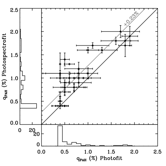
Figure 2.— $q_{\rm PAH}$ from photofit and photospectrofit models. Because of the gridding of the models, a number of points can overlap on this plot. The gray line shows the average offset between the two values excluding the points which have $q_{\rm PAH}$= $0.4$% while the black line shows a one-to-one relationship. Most of the points have a best fit value for $q_{\rm PAH}$ at the lower limit of the model range.

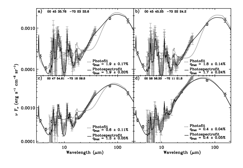
Figure 3.— Four examples of the photofit and photospectrofit models for regions with overlapping photometry and spectroscopy. The IRS spectrum is shown in gray and the MIPS and IRAC photometry are shown with diamond-shaped symbols. For clarity we have not overplotted the model photometry. The photofit model is shown as a dashed black line and the photospectrofit model is shown as a solid black line. The differences between the models represent a redistribution of the radiation field, the parameters of which are listed in Table 5. The R.A. and Dec position of each of these regions is listed in the upper left corner of the plot. Panel d) shows a representative spectrum from the N 66 region.

Table 5Parameters of Selected Photofit and Photospectrofit Models Shown in Figure 3

	Photofit					Photospectrofit
Panel	$\alpha$	Umin	Umax	$\gamma$		$\alpha$	Umin	Umax	$\gamma$
a	1.70 $\pm$ 0.08	3.0 $\pm$ 1.0	7.0	4.9 $\pm 3.8\times 10^{-4}$		1.50 $\pm$ 0.70	2.0 $\pm$ 0.8	3.0	0.1 $\pm 4.1\times 10^{-1}$
b	1.50 $\pm$ 0.04	1.5 $\pm$ 0.5	7.0	2.7 $\pm 2.2\times 10^{-5}$		1.70 $\pm$ 0.41	1.2 $\pm$ 0.2	3.0	0.2 $\pm 3.4\times 10^{-1}$
c	1.80 $\pm$ 0.06	5.0 $\pm$ 1.1	7.0	2.1 $\pm 0.9\times 10^{-3}$		2.30 $\pm$ 0.01	2.0 $\pm$ 0.8	4.0	4.1 $\pm 2.9\times 10^{-1}$
d	2.30 $\pm$ 0.19	5.0 $\pm$ 2.4	7.0	9.0 $\pm 3.0\times 10^{-1}$		2.20 $\pm$ 0.29	3.0 $\pm$ 12.	5.0	1.0 $\pm 0.7\times 10^{0}$

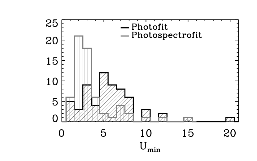
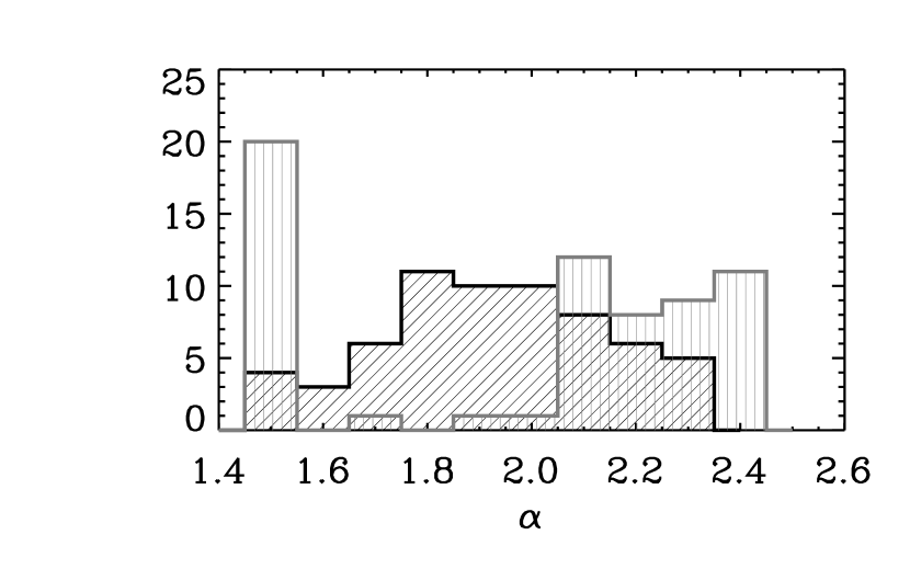
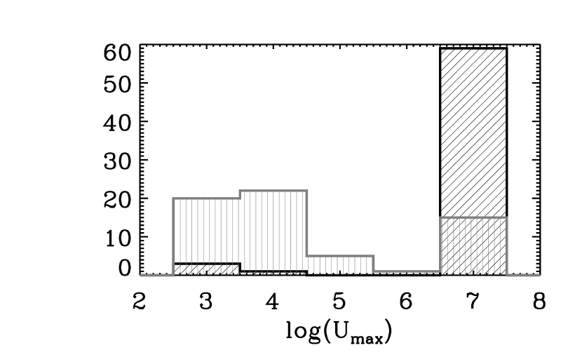
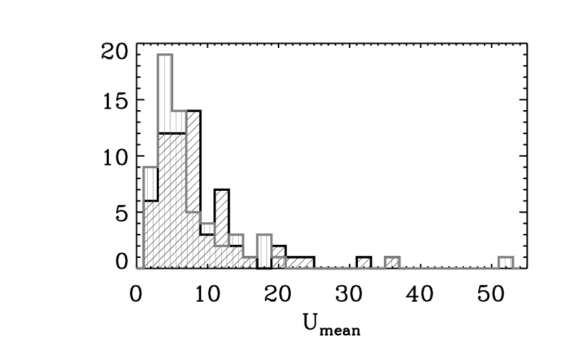
Figure 4.— Histograms illustrating the variation of the radiation field paramters for the photofit models (in black) and photospectrofit models (in gray). The mean radition field ($\bar{U}$) is shown in the lower right panel. Despite the redistribution of the radiation field, the mean field is essentially unchanged in the two best fit models.

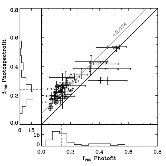
Figure 5.— A comparison of $f_{PDR}$ for the photofit and photospectrofit models. The dashed line on the histograms illustrates the mean of the $f_{PDR}$ values. On average $f_{PDR}$ increases by 0.074 when the spectroscopic information is included in the fit.

As previously discussed, the value of $q_{\rm PAH}$ is essentially proportional to the ratio of the power in the 8 µm PAH emission features to the total far-IR power, and is therefore relatively insensitive to variations in the other fitting parameters. The agreement between the two best fit $q_{\rm PAH}$ values is a strong indication that the technique is robust even though our dust model is not tailored for the SMC and does not have variable band ratios. We note that the spectroscopic maps are preferentially located in star-forming regions, and most cover H II regions. In these spots in particular, the radiation field will deviate the most from the general interstellar field. Over the rest of the SMC, the increase in $f_{PDR}$ will not be as dramatic. We also note that the largest differences in $q_{\rm PAH}$ from the spectoscopic and photometric comparison occur in N 22, which contains a point source that is highly saturated at 24 µm. We have attempted to exclude the regions of N 22 affected by the saturation, but if there were excess 24 µm emission from the PSF wings of this source contaminating the photometry, it may artificially drive up the PDR fraction and change $q_{\rm PAH}$ more drastically.

Our conclusions from the comparison of the photofit and photospectrofit models are that the $q_{\rm PAH}$ values are in agreement. The radiation field parameters from the photospectrofit models reflect a redistribution of the radiation such that the average stays the same while the fraction of dust heated by more intense fields increases and the minimum field decreases. These shifts are most likely not as large in most regions across the SMC as they are in the star-forming regions we probe with spectroscopy. Finally, for regions with intermediate values of $q_{\rm PAH}$ we recognize the fact that we may underestimate the PAH fraction by a few tenths of a percent on average, however this small difference does not affect our conclusions.

4.2. Results of the SED Models Across the SMC

In Figure 6 we show representative SEDs and photofit models from four locations in the SMC and in Figure 7 we show the $q_{\rm PAH}$ from the photofit models at every pixel in our map. All pixels in our map have $q_{\rm PAH}$ less than the average Milky Way value ($q_{\rm PAH,MW}$ = 4.6%). One of the noticable features of this map is the large spatial variations in the PAH fraction, from essentially no PAHs to approximately half the Milky Way PAH fraction in some of the star-forming regions—a range that spans nearly an order-of-magnitude.

The average PAH fraction in the region we mapped is $\langle$$q_{\rm PAH}$$\rangle=0.6$%, determined by the following average:

$$\langle q_{\mathrm{PAH}}\rangle=\frac{\sum_{j}q_{\mathrm{PAH},j}M_{\mathrm{D},j}}{\sum_{j}M_{\mathrm{D},j}}.$$ (4)

Given the minimum value of $q_{\rm PAH}$ allowed by our models, this value is in good agreement with the SW Bar average determined by Li & Draine (2002) but is 8 times lower than the average from Bot et al. (2004).

Previous studies of low metallicity dwarf galaxies have shown large variations in 8 µm surface brightness (e.g. Cannon et al. 2006; Jackson et al. 2006; Hunter et al. 2006; Walter et al. 2007) which we also identify in the SMC. Some of the regions that are brightest at 8 µm have relatively low PAH fractions (c.f. Cannon et al. 2006). To illustrate, we overlay the $q_{\rm PAH}$ map on the IRAC 8 µm mosaic in Figure 8. There are a number of regions where 8 µm emission is very bright while the PAH fraction is low. In particular, N 66 and the Northern region of the SW Bar stand out as very bright 8 µm sources which have relatively low $q_{\rm PAH}$. A representative spectrum of N 66 is shown in the bottom panel of Figure 3, illustrating the low $q_{\rm PAH}$ in this region.

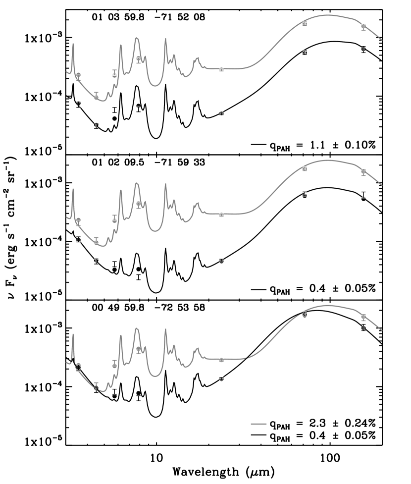
Figure 6.— Comparison of some representative SEDs and photofit models. The positions of these SEDs are marked with square symbols on Figure 7. The gray line appears in each panel for comparison and shows one of the highest $q_{\rm PAH}$ values from the model fits from the SW Bar which is marked on Figure 7 with a black square. The location of the SEDs are listed in the top left of the plot. The measured photometric points are shown with error bars and the synthetic photometry for the best fit model is shown with a filled circle. These panels illustrate the range of $q_{\rm PAH}$ values we see in the SMC.

Figure 7.— This map shows the $q_{\rm PAH}$ values from our fit to the photometry at each pixel in the mapped region (40$\arcsec$ resolution). The outer white boundary shows the overlapping coverage of the MIPS and IRAC mosaics. The white asterisks show the locations of the stars with measured UV extinction curves (Gordon et al. 2003) discussed in Section 4.5. The white squares show the locations of the SEDs plotted in in black in Figure 6. The black square in the SW Bar shows the location of the SED plotted in gray in each panel of Figure 6.

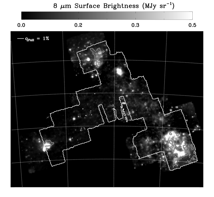
Figure 8.— A map of 8 µm emission overlayed with the 1% contour of $q_{\rm PAH}$. There are a number of regions that are very bright at 8 µm that do not have high PAH fractions, particularly N 66 and the northern part of the SW Bar.

To evaluate the use of the 8/24 ratio as an indicator of PAH fraction, we show in Figure 9 a plot of $q_{\rm PAH}$ vs 8/24, with the average for each value of $q_{\rm PAH}$ overlayed. The PAH fraction is correlated with the 8/24 ratio, even on small scales in the SMC. However, it is evident that the correlation is weak, with a large range in $q_{\rm PAH}$ for a given value of the 8/24 ratio.

The 8/24 ratio spans the region where Engelbracht et al. (2005) see a transition from galaxies with evidence for PAH emission to galaxies which show no PAH features, which is what one would expect given the metallicity of the SMC. The results of our SED modeling indicate that the PAH fraction, though always lower than $q_{\rm PAH}$_,MW, is not uniform across the SMC. There are regions with $q_{\rm PAH}$ within a factor $\sim 2$ of $q_{\rm PAH}$_,MW and regions where $q_{\rm PAH}$ is at the lower limit of the Draine & Li (2007) models ($\sim$ $q_{\rm PAH}$${}_{\rm,MW}/10$). Since there are not comparable resolved maps of $q_{\rm PAH}$ in a sample of galaxies spanning this transition zone, we cannot explain the trend in PAH fractions by looking at the SMC alone. However, the global PAH fraction we measure for the SMC ($\langle$$q_{\rm PAH}$$\rangle\sim 0.6$%) is driven by the very low $q_{\rm PAH}$ over the majority of the galaxy and the large regional variations in $q_{\rm PAH}$ make it unlikely that we are observing a uniform decrease in the SMC PAH fraction. If the SMC is typical of galaxies at this metallicity, the transition represents a decrease in the filling factor of the PAH-rich regions, rather than a uniformly low global PAH fraction.

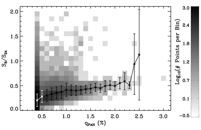
Figure 9.— This figure shows a two-dimensional histogram of the 8/24 ratio vs $q_{\rm PAH}$ overlayed with the binned average of the 8/24 ratio and error bars representing the standard deviation of the scatter at each $q_{\rm PAH}$ bin. The color scale shows the number of points in each bin.

The SED fits provide a number of parameters describing the radiation field. In Figure 10, we show two panels which illustrate the average radiation field $\bar{U}$ and the PDR fraction $f_{PDR}$. Regions where the PDR fraction is high tend to correspond to H II regions, as expected. We overlay representative contours of H$\alpha$ on the map of $f_{PDR}$ and $\bar{U}$ to highlight the brightest H II regions in the Cloud. We also measure the total dust mass and the stellar luminosity at each pixel. We find that the dust mass from our fits agrees well with previous results from Leroy et al. (2007) using the same MIPS observations despite different methodologies. Figure 11 shows a comparison of our dust mass results with those of Leroy et al. (2007) and we find that our masses are lower by $\sim 30$%, well within the $\sim 50$% systematic uncertainties claimed by Leroy et al. (2007).

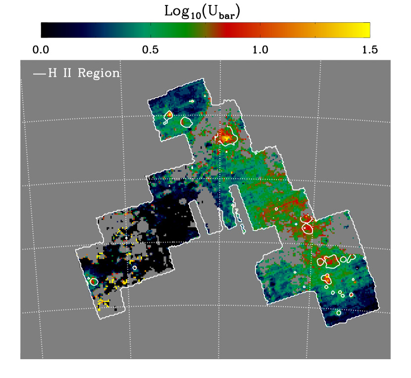
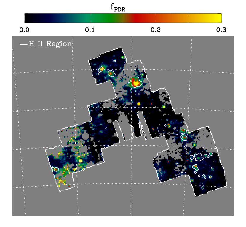
Figure 10.— Maps of the average radiation field ($\bar{U}$) and PDR fraction ($f_{PDR}$) from the photofit models. We have overlayed one representative contour of the MCELS H$\alpha$ image to illustrate the locations of the brightest H II regions in the SMC. The correspondence between $f_{PDR}$ and the location of H II regions is very good, as expected.

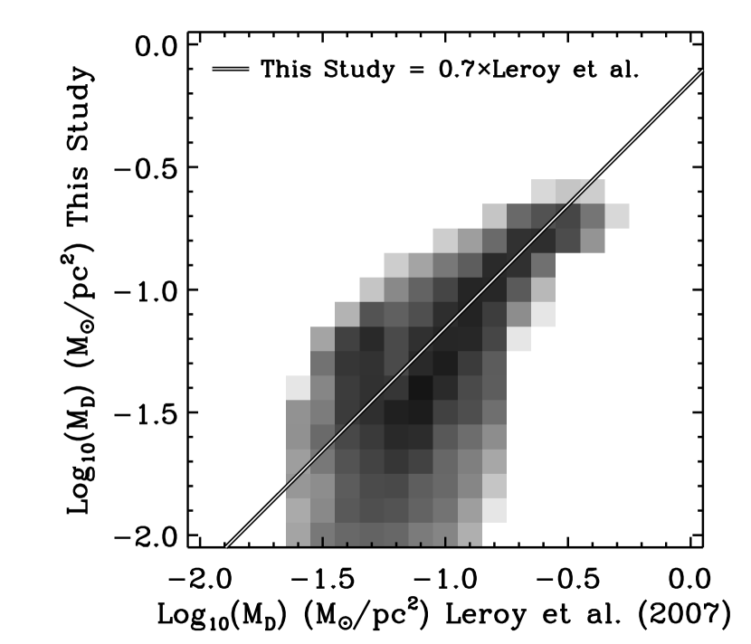
Figure 11.— A two-dimensional histogram showing the comparison of the dust mass surface density M_D from our study with that of Leroy et al. (2007). The gray-scale, with a linear stretch, shows the density of points in the plot. Our M_D is approximately 70% of that found by Leroy et al. (2007), using the same MIPS data but different methodolgy. We note that the scatter at low surface densities likely relates to the fact that we performed our analysis at 40″ resolution but convolved to 2.6′ for comparison with Leroy et al. (2007) and we would expect higher signal-to-noise if the analysis had been performed in the opposite order.

4.3. Spatial Variations in the PAH Fraction

Since we see clear spatial variations in the PAH fraction, we discuss in the following section what sort of conditions foster high PAH fractions in the SMC. We observe three trends: (1) the PAH fraction is high in regions with high dust surface densities and/or molecular gas as traced by CO, (2) the PAH fraction is low in the diffuse interstellar medium and (3) the PAH fraction is depressed in H II regions.

In Figure 12 we show the $q_{\rm PAH}$ map overlayed with contours of ¹²CO (J$=1-0$) emission from the NANTEN survey (Mizuno et al. 2001). There is a strong correlation between the presence of molecular gas and the regions with higher PAH fraction. In Figure 13 we show a histogram of $q_{\rm PAH}$ for lines-of-sight with detected CO emission in the NANTEN map of the SMC and those without. The mean value of $q_{\rm PAH}$ for a line of sight with CO is twice that for a line of sight without CO. In addition, there are no lines of sight through only atomic gas which have $q_{\rm PAH}$ higher than $\sim 1$%. We note that the CO map has much lower resolution than our map of $q_{\rm PAH}$, so the association of PAHs with CO is most likely stronger than the evidence we present here.

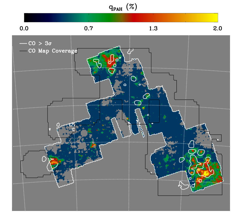
Figure 12.— In this figure we show the $q_{\rm PAH}$ map from Figure 7 with contours of 3$\sigma$ CO (J=1$-$0) emission from the NANTEN survey overlayed. The thin black line represents the coverage of the NANTEN survey. The NANTEN observations have a resolution of 2.6$\arcmin$.

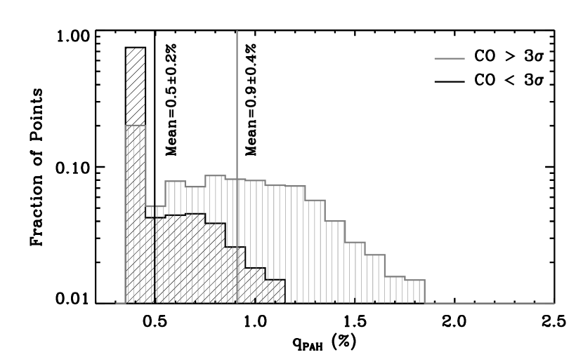
Figure 13.— Histogram of $q_{\rm PAH}$ in lines-of-sight with and without detected CO emission from the NANTEN survey.

The association of PAH emission with star-forming regions and molecular clouds versus the diffuse ISM of a galaxy is a matter of debate, and may vary depending on the galaxy type and star-formation history. Bendo et al. (2008) find that the 8/160 µm ratio in 15 nearby face-on spirals suggests that the PAHs are associated with the diffuse cold dust that produces most of the 160 µm emission. On the other hand, Haas et al. (2002) find that the 8 µm feature, across a range of galaxy type and current star formation rate, is associated with peaks of 850 µm surface brightness, which originate in molecular regions. The distribution of PAHs in a galaxy is one parameter that will help determine what fraction of the PAH luminosity aries from the reprocessing of UV photons from young, hot stars versus the general galactic distribution of B stars. This distinction is crucial in using PAH emission as a tracer of current star-formation (Peeters et al. 2004; Calzetti et al. 2007). To further understand the distribution of PAHs in the SMC, we explore the correlation of PAH fraction with 160 µm emission and the dust mass in Figure 14. In this Figure, we see that the PAH fraction is correlated with dust surface density (M_D) and 160 µm emission, but only weakly correlated with H I column (note that the H I column is shown in a linear scale while M_D and 160 µm emission are shown on a logarithmic scale).

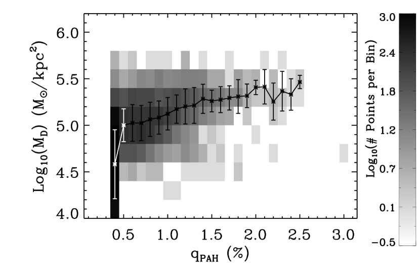
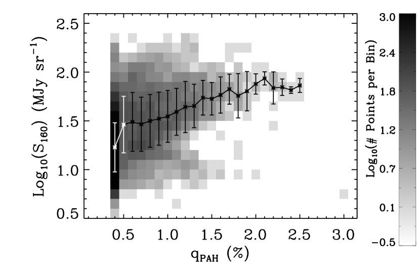
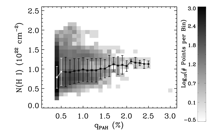
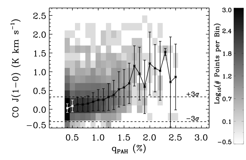
Figure 14.— Two-dimensional histograms of the dust mass surface density, 160 µm surface brightness, neutral hydrogen column and CO integrated intensity as a function of $q_{\rm PAH}$ overlayed with the binned average. The error bars show the standard deviation of the scatter in each bin of $q_{\rm PAH}$. The gray scale represents the logarithm of the number of points in each bin.

The correlation of the PAH fraction with dust surface density but not H I reflects the fact that PAHs are not uniformly distributed in the SMC. Regions with PAH fraction greater than 1% in general have M${}_{D}>10^{5}$ M_⊙ kpc^-2. However, regions with dust surface densities above this level also tend to contain molecular gas, so the dust surface density and H I column no longer track each other because of the presence of H₂ (Leroy et al. 2007). For this reason, we see at best a weak correlation of $q_{\rm PAH}$ with neutral hydrogen column, but a stronger association with CO emission. Bolatto et al 2010 (in prep) have used the MIPS observations of the SMC from S³MC and the SAGE-SMC survey to map the distribution of molecular gas as inferred from regions with “excess” dust surface density relative to the column of neutral hydrogen, using the same techniques as Leroy et al. (2007) and Leroy et al. (2009). In Figure 15 we show their map of the H₂ column density overlayed with a contour at $q_{\rm PAH}$= $1$% and a contour of 3$\sigma$ CO emission. Although we must use caution in comparing the detailed distribution of CO to $q_{\rm PAH}$ since the CO is at $\sim 4$ times lower resolution, it is interesting to note that there are regions with high molecular gas columns without CO and with low PAH fractions, for instance in the northern region of the SW Bar. This may indicate that the radiation field in these regions is affecting both CO and PAHs.

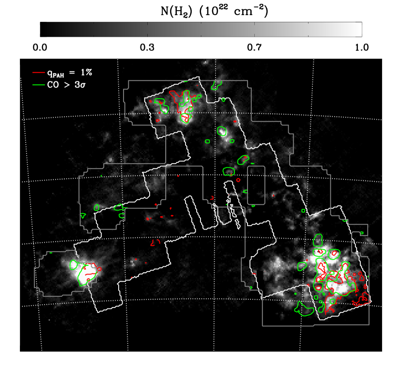
Figure 15.— A map of molecular gas column density inferred from excess dust emission at 160 µm from Bolatto et al 2009 (in prep) overlayed with the 3$\sigma$ contour of CO emission in green and the 1% contour of $q_{\rm PAH}$ in red. The coverage of the CO survey is shown as a thin gray line.

We have so far shown that PAH fraction is high in regions of active star-formation, associated with the presence of CO and molecular gas. PAHs can also be destroyed in regions of active star-formation by the intense UV fields produced by massive stars or in the H II regions themselves by chemistry with H⁺ (Giard et al. 1994). Figure 16 shows the MCELS map of H$\alpha$ in the SMC overlayed with the 1% contour of $q_{\rm PAH}$. From this comparison it is clear that the regions of high PAH fraction are typically on the outskirts of H II regions (i.e. the high $q_{\rm PAH}$ regions and the H II regions are not co-spatial). In particular, the region around N 66, the largest H II region in the SMC, has a very low PAH fraction. We will discuss the influence of H II regions and massive star-formation on the PAH fraction further in Section 5.3.

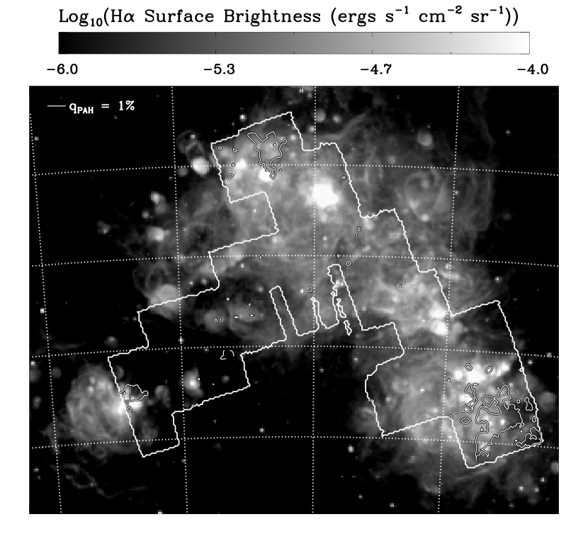
Figure 16.— MCELS H$\alpha$ image with the 1% contour of $q_{\rm PAH}$ overlayed. The regions of high PAH fraction are typically on the outskirts of H II regions.

4.4. The PAH Fraction in SMC B1 # 1

The molecular cloud SMC B1 # 1 was the first location in the SMC where the emission from PAHs was identified (Reach et al. 2000). This region has been studied extensively and the PAH emission spectrum has been modeled by Li & Draine (2002) who found that the PAH fraction in SMC B1 ($q_{\rm PAH}$$\sim 1.6$%) was 8 times higher than the average fraction in the Bar ($q_{\rm PAH}$$\sim 0.2$%). In addition, Reach et al. (2000) and Li & Draine (2002) noted unusual band ratios of the 6.2, 7.7, and 11.3 µm features. In Figure 17 we show the best fit models for the spectrum and photometry of SMC B1. We find $q_{\rm PAH}$$\sim 1.2\pm 0.1$%, in relatively good agreement with Li & Draine (2002) considering the differences in resolution between our respective datasets. We also reproduce the distinctive band ratios (11.3 and 6.2 features high compared to the 7.7 feature) seen with ISO. SMC B1 does not have a uniquely large PAH fraction compared to other locations in the SW Bar.

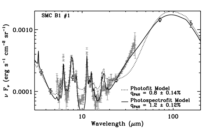
Figure 17.— Best fit models to the photometry and spectroscopy in SMC B1 # 1. The gray points show the IRS spectrum of SMC B1, while the diamonds show the photometry from IRAC and MIPS.

4.5. PAH Fraction and the 2175Å Bump

On Figures 7 and 18 we show the locations of the five stars with measurements of their UV extinction curves with asterisks. Of these stars, only one shows a 2175 Å bump in its extinction curve: AzV 456, which unfortunately lies just outside the boundaries of the map. The lack of a bump in the remaining stars has been interpreted as evidence for a low PAH fraction along those lines-of-sight, assuming that PAHs are the carrier of the bump (Li & Draine 2002). To test this assertion, we list in Table 6 the measured values of E(B$-$V) for the five stars with extinction curves from Gordon et al. (2003) along with the E(B$-$V) and $q_{\rm PAH}$ we calculate from our photofit model results at those positions. For the Draine & Li (2007) models, the dust mass surface density M_D and E(B$-$V) are related by a constant value of $2.16\times 10^{-6}$ mag (M_⊙ kpc^-2)^-1.

The comparison of the E(B$-$V) values shows that the stars are indeed behind the majority of the dust along those lines of sight, and that the $q_{\rm PAH}$ values are slightly above the SMC average of 0.6% (see Section 4.2). A more detailed analysis of these lines-of-sight will be presented in a follow-up paper with targeted IRS spectroscopy to study the PAH emission in these regions. Since we do find that regions of high $q_{\rm PAH}$ tend to be associated with molecular gas, it may be the case that assuming the dust and PAHs are uniformly mixed along each line of sight does not hold. In that case, the comparison of E(B$-$V) values may not be a good indicator of whether these stars should show the 2175 Å bump in their extinction curves. In addition, our angular resolution is not high enough in these maps to directly observe the structure of the dust emission in the vicinity of these stars, so we can not definitively test the PAH-2175 bump connection. We note that one of the stars lies near N 66 in a region with very low ambient PAH fraction. Some of the other stars may fall in voids in the PAH distribution, but higher angular resolution is necessary to understand the line of sight towards these stars.

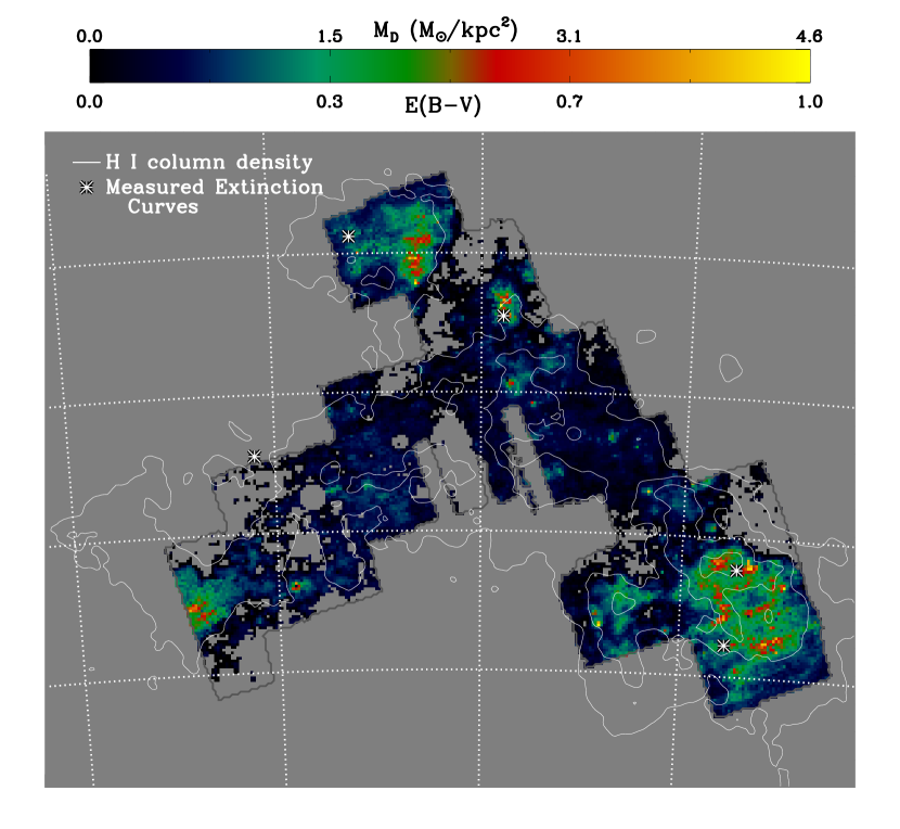
Figure 18.— The dust mass surface density and E(B$-$V) values derived from our photofit models at each pixel overlayed with contours of neutral hydrogen column density from Stanimirovic et al. (1999) at 6, 10, 14 and $18\times 10^{21}$ cm^-2. The locations of the five stars in the SMC with extinction curves from Gordon et al. (2003) are shown with asterisks. Table 6 shows a comparison of the E(B$-$V) measured for those stars with the total line-of-sight E(B$-$V) we calculate from the photofit model results.

Table 6Comparison with Extinction Curve Measurements

Star	R.A.	Dec.	E(B$-$V) (Gordon et al. 2003)	E(B$-$V) (This Study)	$q_{\rm PAH}$
	(J2000)	(J2000)	(mag)	(mag)	(%)
AzV 18	$0^{\rm h}47^{\rm m}12^{\mathrm{s}}$	$-73^{\circ}06\arcmin 33\arcsec$	0.167$\pm$0.013	0.25$\pm$0.07	0.4$\pm$ 0.1
AzV 23	$0^{\rm h}47^{\rm m}39^{\mathrm{s}}$	$-73^{\circ}22\arcmin 53\arcsec$	0.182$\pm$0.006	0.30$\pm$0.10	0.8$\pm$ 0.1
AzV 214	$0^{\rm h}58^{\rm m}55^{\mathrm{s}}$	$-72^{\circ}13\arcmin 17\arcsec$	0.147$\pm$0.012	0.34$\pm$0.13	0.7$\pm$ 0.2
AzV 398	$1^{\rm h}06^{\rm m}10^{\mathrm{s}}$	$-71^{\circ}56\arcmin 01\arcsec$	0.218$\pm$0.024	0.33$\pm$0.09	0.8$\pm$ 0.1
AzV 456	$1^{\rm h}10^{\rm m}56^{\mathrm{s}}$	$-72^{\circ}42\arcmin 56\arcsec$	0.263$\pm$0.016	$\cdots$	$\cdots$

Note. — The E(B$-$V) calculations are described in Section 4.5.

5. What Governs the PAH Fraction in the SMC?

Draine et al. (2007) determined the PAH fraction in the SINGs galaxy sample using identical techniques to what we have done here. They observed a effect very similar to what was seen by Engelbracht et al. (2005) in that at a metallicity of $12+$ log(O/H) $\sim 8.0$ there is an abrupt change in the typical PAH fraction or 8/24 µm ratio. The SMC lies right at this transition metallicity, so we hope to gain some insight into the processes at work by studying its PAH fraction. There is still a great deal of uncertainty as to how PAHs form and how they are destroyed, let alone how those processes balance in the ISM. In the following sections we address some of the proposed aspects of the PAH life-cycle and elucidate what we can learn about them from the SMC.

5.1. Formation by Carbon-Rich Evolved Stars

The formation of PAHs in the atmospheres of evolved stars is a well established hypothesis for the source of interstellar PAHs. PAH emission bands have been observed in the spectrum of the carbon-rich post-AGB stars where the radiation field increases in hardness and intensity, more effectively exciting the PAH emission features (Justtanont et al. 1996). Despite these observations of PAH formation in carbon-rich stars, it remains to be shown that they inject PAHs into the ISM at the level needed to explain the abundance observed. This, of course, is a general problem in the “stardust” scenario (Draine 2009). Recently, in the Large Magellanic Cloud, Matsuura et al. (2009) have performed a detailed accounting of the dust enrichment of the ISM by AGB stars and find a significant deficit compared to the observed ISM dust mass.

Assuming that the “stardust” picture is correct, Galliano et al. (2008) and Dwek (1998) hypothesize that the low fraction of PAHs in low metallicity galaxies reflects the delay ($\sim 500$ Myr) in the production of carbon dust from AGB stars relative to silicate dust from core-collapse supernova. For the SMC in particular, this picture has a number of issues. Most importantly, there is evidence that the SMC formed a large fraction of its stars more than 8 Gyr ago followed by a subsequent burst of star formation 3 Gyr ago (Harris & Zaritsky 2004). This long time scale makes the delayed PAH injection into the ISM by AGB stars an unlikely explanation for the current observed PAH deficiency. Recent work by Sloan et al. (2009), for example, argues that carbon-rich AGB stars in low metallicity galaxies can start contributing dust to the ISM in $\sim 300$ Myr.

To evaluate the relationship between the current distribution of PAHs and the input of PAHs from AGB stars, we show in Figure 19 the PAH fracion overlayed with contours of the density of carbon AGB stars. These contours are created using the 2MASS 6X point source catalog towards the SMC, selecting carbon stars using the technique described in Cioni et al. (2006). The distribution of carbon stars follows the observed “spheroidal” population of older stars in the SMC very well (Zaritsky et al. 2000; Cioni et al. 2000). The $q_{\rm PAH}$ map, however, has no clear relationship to the distribution of carbon stars. This is perhaps to be expected since the distribution of ISM mass does not follow the stellar component either. However, we note that a different conclusion regarding the PAH fracion compared to the distribution of AGB stars was recently reached by Paradis et al. (2009), who modeled dust SEDs across the Large Magellanic Cloud using the SED models of Desert et al. (1990). They find evidence that the fracion of PAHs in the LMC is highest in the region of the stellar bar, where the concentration of AGB stars peaks. This could be an accidental coincidence, or it may reflect methodological differences or it could indicate a different dominant mechanism of PAH formation in the SMC and LMC or more efficient destruction of PAHs in the SMC.

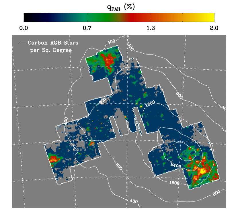
Figure 19.— Map of $q_{\rm PAH}$ overlayed with contours of carbon AGB star density determined from the 2MASS 6X point source catalog using the selection criteria of Cioni et al. (2006). The contours are labeled with the density of carbon stars per square degree. There is no obvious correspondence between the distribution of carbon stars and the fraction of PAHs.

Although the distribution of PAHs may not resemble that of AGB stars, we would expect the PAHs injected by those stars to be present in the diffuse ISM and not preferentially in molecular clouds. As we have shown, however, the diffuse ISM PAH content is very low in the SMC. As such, in order to reconcile the pathway of PAHs from AGB stars to the diffuse ISM to molecular clouds, we must hypothesize a recent event, occuring after the condensation of the current generation of molecular clouds, which essentially cleared the diffuse ISM of AGB-produced PAHs while leaving the shielded regions of molecular gas with high PAH fractions. Observations of giant molecular clouds (GMCs) in the Magellanic Clouds and other nearby galaxies suggest that the GMC lifetime is $\sim 25$ Myr (Fukui et al. 1999; Blitz et al. 2007), so the event in question would have had to occur within the last 25 Myr or so. In the absence of such an event (which we will investigate further in a Section 5.3), our observation of low PAH fraction in the diffuse ISM, higher PAH fraction in molecular clouds, and the lack of relation between the PAH fraction and the distribution of AGB stars is strong evidence against AGB stars being the dominant force behind the fraction of PAHs in the SMC.

5.2. Formation and Destruction of PAHs in Shocks and Turbulence

The shocks created by supernova explosions have a dramatic effect on the content and size distribution of dust in the interstellar medium. Upon encountering a shock wave, grains can be shattered via collisions or sputtered by hot gas behind the shock or by motion of the grain through the post-shock medium. Because of their small mass-to-area ratio, PAHs are well coupled to the gas and do not acquire large relative velocities after the passage of a shock, so they will primarily be sputtered only in hot post-shock gas behind fast ($v>200$ km s^-1) shocks. Calculations by Jones et al. (1996) suggest that grain shattering could in fact be a net source of PAH material for shocks between 50 and 200 km s^-1, converting $\sim 10$% of the initial grain mass into small PAH sized fragments. Thus, it is not immediately obvious what the net effect of interstellar shocks on the fraction of PAHs will be.

Some studies attribute the low PAH fraction in low metallicity galaxies to efficient destruction of PAHs by supernova shocks. O’Halloran et al. (2006) found a correlation between decreasing PAH emission and increased supernova activity as traced by the ratio of mid-IR lines of [Fe II] and [Ne II]. Two issues with this interpretation are that the mid-IR lines are tracing current supernova activity, which only affects the PAH fraction in the immediate vicinity of those remnants, and an increased supernova rate will have recently been related to a higher UV field produced by the massive stars, so it is difficult to disentangle the effects of shocks versus intense UV fields.

The distinctive nature of the SMC extinction curve might point toward the influence of supernova shocks on the dust grain size distribution. Four of the five extinction curves show similar characteristics: a lack of the 2175 Å bump (the carrier of which is most likely PAHs Li & Draine 2001) and a steeper far-UV rise indicating more small dust grains relative to the Milky Way extinction curve (Gordon et al. 2003; Cartledge et al. 2005). Magellanic-type extinction has been seen to arise in the Milky Way as well along the sightline towards HD 204827, which may be embedded in dust associated with a supernova shock (Valencic et al. 2003). However, there are many other viable interpretations to explain the proportion of small dust grains, including inhibition of grain growth in dense clouds.

In Figure 20 we show a map of the H I velocity dispersion in the SMC from Stanimirovic et al. (1999). The velocity dispersion here mostly traces the regions where there are more than one velocity component along the line of sight, particularly highlighting the regions where Stanimirovic et al. (1999) find evidence for supergiant shells in the H I distribution. We show the approximate locations of two of their shells that overlap our map. If supernovae are the source of these shells, Stanimirovic et al. (1999) find that $\sim 1000$ supernovae are required to account for the kinetic energy and the shells have dynamical ages of $\sim 20$ Myr. The supergiant shells provide indirect evidence for the effects of supernovae on the ISM. On Figure 20 we also mark with green crosses the locations of young ($\sim 1000-10000$ yr) supernova remnants identified in the Australia Telescope Compact Array survey of the SMC (Payne et al. 2004).

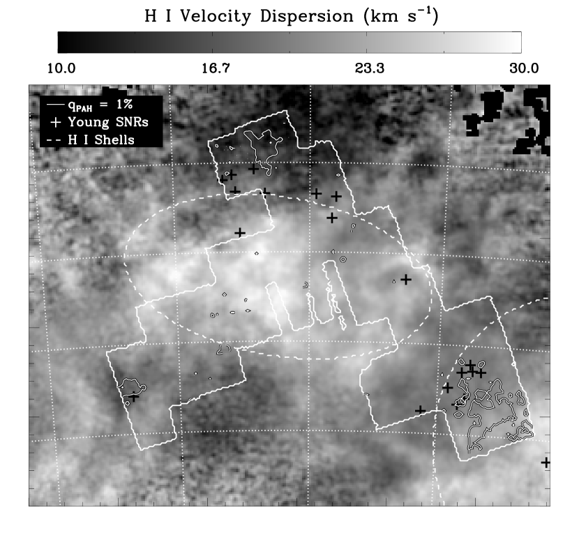
Figure 20.— SMC H I velocity dispersion from Stanimirovic et al. (1999). The approximate locations of the supergiant H I shells identified by Stanimirovic et al. (1999) are shown with a dashed white line. The velocity dispersion mainly traces bulk motions of gas along the line of sight, particularly highlighting the regions of these shells. We show the locations of young supernova remnants identified in the ATCA survey of the SMC with black crosses.

There is no clear trend relating $q_{\rm PAH}$ to the boundaries of the supergiant shells, although this may be an effect of depth along the the line of sight. The middle region of the Bar and Wing, which is essentially devoid of PAHs is covered by one of the shells, but the SW Bar, which hosts the largest concentration of PAHs in the SMC is covered as well. Although there is an anticorrelation between the young SNRs and large PAH fraction, the distribution of remnants closely follows that of the massive star-forming regions (compare Figures 16 and 20). For this reason, it is difficult to draw strong conclusions as to whether the supernova shocks or the UV fields and H II regions created by their progenitor stars were responsible for destroying PAHs in these areas.

Similar to shocks, regions of high turbulent velocity may alter the size distribution of dust grains via shattering. Miville-Deschênes et al. (2002) studied a region of high latitude cirrus and argued that variations in small dust grain and PAH fractions could be related to the turbulent velocity field in the region. Burkhart et al. (2010) have studied turbulence in the ISM of the SMC using the H I observations of Stanimirovic et al. (1999). They present a map showing an estimate of the sonic Mach number of turbulence in the SMC based on higher order moments of H I column density and the results of numerical simulations. This map is quite distinct from the velocity dispersion map shown in Figure 20 which mostly highlights the presence of bulk velocity motions along the line of sight. In Figure 21 we show the Burkhart et al. (2010) Mach number map overlayed with the contours of $q_{\rm PAH}$. We find that there is no strong correlation between tubulent Mach number and $q_{\rm PAH}$, although in general the regions of high $q_{\rm PAH}$ are near depressions in the Mach number distribution, opposite what we would expect if grain shattering in turbulence was a major source of PAHs. However, this simple comparison does not provide information about the amount of dust affected by different levels of turbulence (e.g. some of the low Mach number regions may represent a very small fraction of the total ISM). To account for this fact, we also calculate the dust mass surface density weighted Mach number in regions with $q_{\rm PAH}$$>1$% and $<1$% to be $0.8\pm 0.3$ and $1.0\pm 0.4$, respectively. Although there is no clear association between high sonic Mach number and $q_{\rm PAH}$ from this comparison, it is worth noting that if PAHs are primarily associated with molecular gas, the Mach number derived from H I observations may have little relevance to the creation or destruction of PAHs in the SMC.

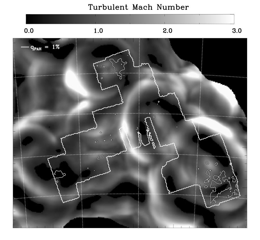
Figure 21.— Map of estimated turbulent Mach number from Burkhart et al (2009) in prep, overlayed with the 1% contour of $q_{\rm PAH}$. The Mach number map has an angular resolution of $30\arcmin$.

In general, we do not see clear cut evidence that turbulence or shocks are the major drivers of the PAH fraction in the SMC. Young SNRs are found around H II regions, making it difficult to separate the effects of radiation field and shocks in the destruction of PAHs in those regions. The supergiant H I shells observed in the SMC may be a tracer of where supernova shocks have seriously affected the ISM, but we see peaks of $q_{\rm PAH}$ within their boundaries barring a line-of-sight depth effect.

5.3. Destruction of PAHs by UV Fields

In low metallicity galaxies, the dust to gas ratio is decreased (Lisenfeld & Ferrara 1998) and the effects of the UV field from regions of massive star formation can be spread over a much larger area. In addition, the decreased metallicity may lead to harder UV fields because of the lower line blanketing in stellar atmospheres. These changes can be traced by the ratios of mid-IR emission lines and work by Madden (2000) and others have shown that radiation fields are harder in low metallicity environments. Gordon et al. (2008) studied star-forming regions in M 101, over a range of excitation conditions and metallicities. They found that the strength of PAH emission decreases with increasing ionization parameter, suggesting that processing by the UV field from these regions was the major force behind the changing PAH fraction.

The exact mechanism of PAH destruction by UV fields is not entirely clear. Small PAHs can be destroyed by the ejection of an acetylene group upon absorbing a UV photon (Allain et al. 1996a), but PAHs larger than $\sim 50$ carbon atoms are relatively stable to these effects under a range of UV field conditions. If the PAHs are partially dehydrogentated or highly ionized, they are more susceptible to destruction (Allain et al. 1996b), so one possibility is that PAHs in low metallicity galaxies tend to be more highly ionized, dehydrogenated or smaller than their counterparts in higher metallicity galaxies. However, there is little evidence from the spectra of low metallicity galaxies (Engelbracht et al. 2008; Smith et al. 2007) that PAHs are different at low metallicity.

There is also a distinction to be made between the destruction of PAHs by intense radiation fields in the immediate vicinity of H II regions and a global decrease of the PAH fraction in the galaxy. We see evidence for PAH destruction near H II regions in our map (see Figure 16). But can UV fields from massive star forming regions be responsible for the low $q_{\rm PAH}$ over the entire galaxy? There is evidence that star-forming regions in irregular galaxies can “leak” a large fraction of their ionizing photons. Observations of emission line ratios from the diffuse ionized gas (DIG) in star-forming dwarfs indicate that dilution of radiation from a central massive star-forming region which leaks a significant fraction of its ionizing photons is a likely source for the DIG (Martin 1997). In the SMC, models of N 66 suggest that $\sim$ 45% of the ionizing photons escape the H II region and go on to ionize the diffuse ISM (Relaño et al. 2002). Thus, it is at least plausible that UV fields may be an important driver of PAH destruction over the entire galaxy.

To evaluate the possibility that the low $q_{\rm PAH}$ in the SMC is due to destruction by UV fields, we examine the resolved star-formation history of Harris & Zaritsky (2004) to search for recent star-forming events that could have affected the PAH fraction in the diffuse ISM through their UV fields. In Figure 22 we show five panels illustrating the Harris & Zaritsky (2004) results regridded to match our map of $q_{\rm PAH}$. These panels show the total star formation rate for bins older than 1 Gyr, from 400 Myr to 1 Gyr ago, from 100 to 400 Myr ago, from 25 to 100 Myr ago and younger than 25 Myr.

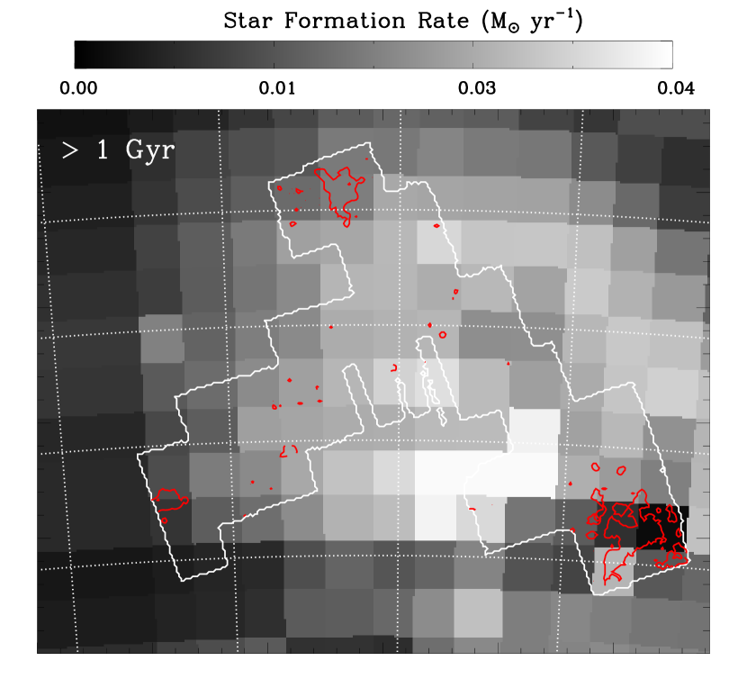
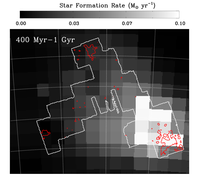
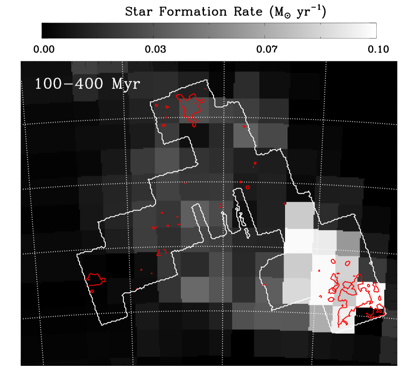
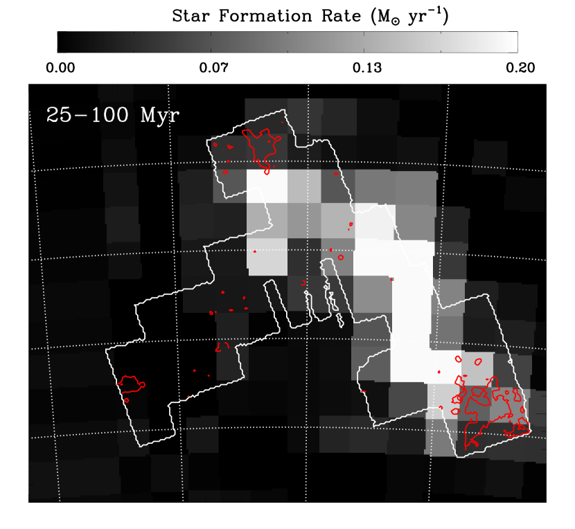
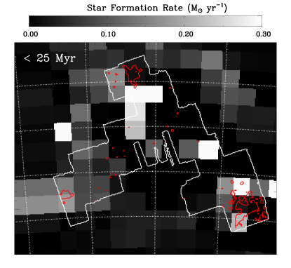
Figure 22.— Resolved star-formation history of the SMC from Harris & Zaritsky (2004). The time-ranges are listed in the upper left corners of each image.

In general, panels which show the star-formation rate in bins older than 100 Myr tend to follow the spheroidal distribution of older stars, as traced by the carbon stars shown in Figure 19. The $25-100$ Myr panel shows that star formation occurred along the Bar, coinciding with the region in our $q_{\rm PAH}$ map that is devoid of PAHs. The most recent star formation, which would overlap the time when the current generation of molecular clouds condensed, seems to be mainly associated with the outermost edges of the Bar, near where we see PAHs.

PAH destruction as a side effect of massive star formation is difficult to disentangle since the UV fields and subsequent supernovae only affect the dust over a short period of time surrounding the star formation event. Between 25 and 100 Myr ago in the SMC, the star-formation along the Bar, which most likely relates to the supergiant bubble seen in the H I overlapping that location, may have cleared the region of PAHs by some combination of UV fields and shocks. However, most of this activity likely occured before the condensation of the molecular clouds ($\sim 25$ Myr $>$ ago; Fukui et al. 1999; Blitz et al. 2007; Kawamura et al. 2009) that currently have a high PAH fraction, so there is still difficulty in reconciling the high $q_{\rm PAH}$ in molecular clouds and the low $q_{\rm PAH}$ in the diffuse ISM by destruction alone.

5.4. The Formation of PAHs in Molecular Clouds

One of our primary observations in the SMC is that high PAH fractions occur along lines of sight through molecular gas. We argue that such a situation could arise in two scenarios: 1) AGB stars enrich the diffuse ISM with PAHs, part of which is then incorporated into molecular clouds. A subsequent event (e.g. SN) clears the PAHs in the diffuse ISM. Or, 2) PAH formation occurs in the molecular clouds. These two scenarios are not mutually exclusive. Paradis et al. (2009) found enhanced PAH fraction in the LMC both in the stellar bar, which hosts the highest concentration of AGB stars, and in molecular clouds. It is possible that in the diffuse ISM of the SMC, AGB produced PAHs are rapidly destroyed and all we observe are PAHs that formed in molecular clouds.

Greenberg et al. (2000) propose a scenario by which PAHs could be formed in dense clouds. They argue that a layer of ices and organic material forms on grains in dense clouds and the photoprocessing which occurs in the transition from the dense cloud back to the diffuse ISM forms PAHs, a phenomenon they explore through laboratory experimentation. There is also observational evidence that hints at some of the processing PAHs undergo in dense clouds. Rapacioli et al. (2005) and Berné et al. (2007) show variations in the PAH spectrum in photo-dissociation regions consistent with PAHs being in clusters or embedded in a carbonaceous matrix in the surrounding molecular gas and emerging as free-flying PAHs closer to the exciting star.

While it would not be out of question that a burst of star-formation $\sim 25$ Myr ago could have a dramatic effect on the global diffuse ISM of the SMC, a more likely scenario for the concentration of PAHs in molecular clouds is that they form there. Assuming that is the case there are a number of interesting observations that we can make about the formation of PAHs in molecular clouds in the SMC. First, the correspondence between the CO and $q_{\rm PAH}$ is very good, better even then the correspondence between the PAHs and the Bolatto et al 2009 (in prep) map of molecular hydrogen inferred from excess dust emission. This suggests that the conditions for the formation of CO and the formation of PAHs are similar. It may be that the UV field in the outskirts of the clouds, where H₂ can self-shield but CO is dissociated, can disrupt the growth of mantles on the grains, preventing a process that creates PAHs. Alternatively, because the growth of mantles requires relatively high densities, the presence of CO may allow the gas to cool and become denser, increasing the rate of gas-grain reactions. This scenario could be tested by comparing the distribution of CO and PAHs in a sample of irregular galaxies. Leroy et al. (2009) found that CO in the N 83 region of the SMC is found where A${}_{V}>2$ through the cloud (A${}_{V}>1$ at cloud center). If CO survives and PAHs form at a similar extinction, the decrease in the PAH fraction and the deficit of CO emission at low metallicity may be related to the scarcity of regions where this condition is met.

Second, we observe that the typical $q_{\rm PAH}$ in SMC molecular clouds is $\sim 1-2$%. This is lower than the average Milky Way value (which is for the diffuse ISM) and may represent some limit on the efficiency of creating PAHs in molecular gas in the SMC. In the low metallicity galaxies studied by Draine et al. (2007), those with metallicities below $12+$ log(O/H) $\sim 8$ had a median PAH $q_{\rm PAH}$ of 1% with large scatter. This scatter could be due to the filling factor of molecular gas. If PAHs are forming primarily in molecular clouds, the differences observed in the PAH fraction in low versus high metallicity galaxies may be related to the ability of PAHs to survive and accumulate in the diffuse ISM and/or to the efficiency of PAH formation in molecular gas, which can be decreased by the lower carbon abundance and the more pervasive UV fields in low metallicity environments.

Finally, in the scenario where PAHs are destroyed in the diffuse ISM and formed in molecular clouds and AGB stars, the abrupt transition at a metallicity of $12+$ log(O/H) $\sim 8$ would represent mostly a change in the efficiency of PAH destruction in the diffuse ISM. If PAHs are destroyed efficiently in the diffuse ISM of these systems, all that is left are the PAHs created in molecular clouds. A resolved study of the PAH abundance in the SINGs galaxies using higher resolution far-IR and millimeter-wave CO observations from Herschel may be able to show whether the PAH fraction in the diffuse ISM versus molecular clouds is changing across the transition metallicity.

6. Summary & Conclusions

We present results of fitting the Draine & Li (2007) dust models to SEDs and spectra obtained from S³MC and S⁴MC. Our major results are as follows:

1. Comparisons of best-fit dust models in regions with overlapping photometry and spectroscopy demonstrate that the IRAC and MIPS SED estimator for $q_{\rm PAH}$ does not appear to be appreciably biased despite the absence of information between $8-24$ and $24-70$ µm. When $5-38$ µm IRS spectroscopy is added to the fitting constraints, the resulting “photospectrofit” models yield $q_{\rm PAH}$ values that are only slightly larger than the “photofit” model estimates. The photospectrofit models have more dust at intermediate (T $\approx 60$K) temperatures, and less dust with T $\approx 200$ K. The estimate for the average radiation intensity scale factor $\bar{U}$ and the dust surface density M_D are nearly unaffected.

2. The PAH fraction in the SMC is low and variable. As a fraction of the total dust mass, the highest PAH fractions we observe are about half of the Milky Way value, but most of the galaxy has PAH fractions at the lower limit of our models ($q_{\rm PAH}$= $0.4$%), an order of magnitude lower than the Milky Way value. The average $\langle$$q_{\rm PAH}$$\rangle\sim 0.6$% in the SMC. This is consistent with the earlier estimate of a very low PAH fraction in the SMC (Li & Draine 2002) based on IRAS and DIRBE photometry.

3. The 8 µm emission alone does not trace the $q_{\rm PAH}$ well in the SMC. We find that the 8/24 ratio is correlated with $q_{\rm PAH}$ and agrees with what one would predict from the metallicity of the SMC and the observed trends in Engelbracht et al. (2005), but for a given $q_{\rm PAH}$ there is a wide range of 8/24 ratios, depending on the intensity of the local starlight heating the grains.

4. The metallicity of the SMC places it at the transition where lower metallicity galaxies show a deficiency of PAHs and higher metallicity galaxies show approximately Milky Way level PAH fractions. If the SMC is typical of galaxies in this region, the transition seems to represent a decrease in the filling factor of PAH-rich regions rather than a uniform decrease in the PAH fraction throughout the galaxy, although even the highest PAH fractions are still well below MW levels.

5. Lines-of-sight with molecular gas have an average $q_{\rm PAH}$ of $\sim 1$%, while lines of sight through the diffuse ISM have $q_{\rm PAH}$ at least a factor of two less.

6. We evaluate the various proposed drivers of the deficit of PAHs at low metallicity. The distribution of PAHs in the SMC does not follow the carbon AGB star distribution, the regions of high turbulent Mach number, or the location of supergiant shells in the ISM.

7. The low PAH fraction in the diffuse ISM versus the high PAH fraction in molecular regions leads us to propose that PAHs may be forming in molecular clouds and/or a recent event (perhaps related to star formation events in the last $\sim$ 25 Myr) destroyed a large fraction of the PAHs in the diffuse ISM.

8. We surmise that the global PAH fraction at low metallicities is a reflection of the amount of gas in these systems that is found at high extinction (A${}_{V}>1$).

.1. Cross-Calibration of MIPS, IRAC and IRS

Because we combine photometry and spectroscopy in our model fitting, we investigated whether there were systematic differences between the calibrations of the IRS and MIPS/IRAC instruments. The SSC finds the cross-calibration agrees to within 10% for the three instruments. However, most of these tests have been carried out on stellar sources, whereas our observations are primarily concerned with extended emission. We have used the extended source corrections for IRAC determined by Reach et al. (2005) and the slit loss correction function for IRS distributed with Cubism.

We have constructed 8 and 24 µm maps from the spectral cubes using the most recent versions of the spectral response curves available from the SSC (for IRAC; Hora et al. 2008). We then compare the IRS 8 and 24 µm maps to the same regions in the IRAC and MIPS mosaic after smoothing to eliminate any small PSF differences between the two instruments. Calibration differences between the instruments present themselves as a non-unity slope in the comparison of IRS 24 µm to MIPS 24 µm and IRS 8 µm to IRAC 8 µm. For the 8 µm comparison, we find that the IRS photometry is higher than the IRAC photometry by factor of 1.1, on average, although the slope in individual regions varies between 1.04 to 1.14. At 24 µm  the IRS photometry is lower than the MIPS photometry by a factor of 0.94 on average, varying between 0.91 and 0.96 region to region. Individually, these differences are within the quoted cross-calibration limits stated by the SSC, however without correction they introduce scatter in the comparison of spectroscopically and photometrically determined $q_{\rm PAH}$.

In addition to the slope, there is an additive offset between the IRS and MIPS/IRAC photometry that is too large to be an issue with the MIPS/IRAC mosaic foreground subtraction described previously (additive offsets are $\sim 0.1-1$ MJy sr^-1 at 24 µm and $\sim 0.01-0.1$ MJy sr^-1 at 8 µm). The source of this additive offset is not definitively known, but we consider it very likely that it results from slight under or over subtraction of the zodiacal light foreground as determined by SPOT for the IRS cubes. The uncertainties of the DIRBE model are on the order of a few percent at the DIRBE wavelengths, and particularly at 24 µm where the zodiacal foreground is very bright (on the order of tens of MJy sr^-1) and a few percent error easily translates into offsets on the order of a few tenths of a MJy sr^-1. In order to eliminate these offsets, we must make some assumption about the spectral shape of the correction. To do this we fix the “off” position zodiacal spectrum and determine the percentage by which the “map” position spectrum must be off to produce the offsets we observe. We do this for each AOR in the dataset and then add in the resulting correction spectrum. The correction is less than 5% in all cases.

The multiplicative differences in the calibration between IRS and MIPS most likely result from the extended source calibration in IRS, since MIPS does not require such a correction. For the IRAC/IRS match-up, the source is not obvious, since both instruments require an extended source correction factor. A further consideration in our work is that we must apply a correction factor consistently across either all of the IRS or all of the IRAC data, since we only have overlapping information in a few regions, but we aim to determine the PAH fractions over the whole S³MC map. There is no obvious way to decide which to correct, the IRS or IRAC calibration, so we choose the simplest route: we apply corrections to the IRS spectra based on the factors necessary to match IRAC 8 µm and MIPS 24 µm. We determine a correction factor that depends linearly on wavelength which matches the photometric to spectroscopic points in each region. This correction factor is very small in the region of the SL1/LL2 overlap, so it does not affect our stitching of the orders.

References

- Allain et al. (1996a) Allain, T., Leach, S., & Sedlmayr, E. 1996a, A&A, 305, 602
- Allain et al. (1996b) —. 1996b, A&A, 305, 616
- Allamandola et al. (1989) Allamandola, L. J., Tielens, A. G. G. M., & Barker, J. R. 1989, ApJS, 71, 733
- Arendt et al. (1998) Arendt, R. G., Odegard, N., Weiland, J. L., Sodroski, T. J., Hauser, M. G., Dwek, E., Kelsall, T., Moseley, S. H., Silverberg, R. F., Leisawitz, D., Mitchell, K., Reach, W. T., & Wright, E. L. 1998, ApJ, 508, 74
- Bakes & Tielens (1994) Bakes, E. L. O., & Tielens, A. G. G. M. 1994, ApJ, 427, 822
- Bakes & Tielens (1998) —. 1998, ApJ, 499, 258
- Bendo et al. (2008) Bendo, G. J., Draine, B. T., Engelbracht, C. W., Helou, G., Thornley, M. D., Bot, C., Buckalew, B. A., Calzetti, D., Dale, D. A., Hollenbach, D. J., Li, A., & Moustakas, J. 2008, MNRAS, 389, 629
- Bernard et al. (2008) Bernard, J.-P., Reach, W. T., Paradis, D., Meixner, M., Paladini, R., Kawamura, A., Onishi, T., Vijh, U., Gordon, K., Indebetouw, R., Hora, J. L., Whitney, B., Blum, R., Meade, M., Babler, B., Churchwell, E. B., Engelbracht, C. W., For, B.-Q., Misselt, K., Leitherer, C., Cohen, M., Boulanger, F., Frogel, J. A., Fukui, Y., Gallagher, J., Gorjian, V., Harris, J., Kelly, D., Latter, W. B., Madden, S., Markwick-Kemper, C., Mizuno, A., Mizuno, N., Mould, J., Nota, A., Oey, M. S., Olsen, K., Panagia, N., Perez-Gonzalez, P., Shibai, H., Sato, S., Smith, L., Staveley-Smith, L., Tielens, A. G. G. M., Ueta, T., Van Dyk, S., Volk, K., Werner, M., & Zaritsky, D. 2008, AJ, 136, 919
- Berné et al. (2007) Berné, O., Joblin, C., Deville, Y., Smith, J. D., Rapacioli, M., Bernard, J. P., Thomas, J., Reach, W., & Abergel, A. 2007, A&A, 469, 575
- Blitz et al. (2007) Blitz, L., Fukui, Y., Kawamura, A., Leroy, A., Mizuno, N., & Rosolowsky, E. 2007, in Protostars and Planets V, ed. B. Reipurth, D. Jewitt, & K. Keil, 81–96
- Bolatto et al. (2007) Bolatto, A. D., Simon, J. D., Stanimirović, S., van Loon, J. T., Shah, R. Y., Venn, K., Leroy, A. K., Sandstrom, K., Jackson, J. M., Israel, F. P., Li, A., Staveley-Smith, L., Bot, C., Boulanger, F., & Rubio, M. 2007, ApJ, 655, 212
- Bot et al. (2004) Bot, C., Boulanger, F., Lagache, G., Cambrésy, L., & Egret, D. 2004, A&A, 423, 567
- Boulanger et al. (1996) Boulanger, F., Abergel, A., Bernard, J.-P., Burton, W. B., Desert, F.-X., Hartmann, D., Lagache, G., & Puget, J.-L. 1996, A&A, 312, 256
- Burkhart et al. (2010) Burkhart, B., Stanimirović, S., Lazarian, A., & Kowal, G. 2010, ApJ, 708, 1204
- Buss et al. (1993) Buss, Jr., R. H., Tielens, A. G. G. M., Cohen, M., Werner, M. W., Bregman, J. D., & Witteborn, F. C. 1993, ApJ, 415, 250
- Calzetti et al. (2007) Calzetti, D., Kennicutt, R. C., Engelbracht, C. W., Leitherer, C., Draine, B. T., Kewley, L., Moustakas, J., Sosey, M., Dale, D. A., Gordon, K. D., Helou, G. X., Hollenbach, D. J., Armus, L., Bendo, G., Bot, C., Buckalew, B., Jarrett, T., Li, A., Meyer, M., Murphy, E. J., Prescott, M., Regan, M. W., Rieke, G. H., Roussel, H., Sheth, K., Smith, J. D. T., Thornley, M. D., & Walter, F. 2007, ApJ, 666, 870
- Cannon et al. (2006) Cannon, J. M., Smith, J.-D. T., Walter, F., Bendo, G. J., Calzetti, D., Dale, D. A., Draine, B. T., Engelbracht, C. W., Gordon, K. D., Helou, G., Kennicutt, Jr., R. C., Leitherer, C., Armus, L., Buckalew, B. A., Hollenbach, D. J., Jarrett, T. H., Li, A., Meyer, M. J., Murphy, E. J., Regan, M. W., Rieke, G. H., Rieke, M. J., Roussel, H., Sheth, K., & Thornley, M. D. 2006, ApJ, 647, 293
- Cartledge et al. (2005) Cartledge, S. I. B., Clayton, G. C., Gordon, K. D., Rachford, B. L., Draine, B. T., Martin, P. G., Mathis, J. S., Misselt, K. A., Sofia, U. J., Whittet, D. C. B., & Wolff, M. J. 2005, ApJ, 630, 355
- Cherchneff et al. (1992) Cherchneff, I., Barker, J. R., & Tielens, A. G. G. M. 1992, ApJ, 401, 269
- Cioni et al. (2006) Cioni, M.-R. L., Girardi, L., Marigo, P., & Habing, H. J. 2006, A&A, 452, 195
- Cioni et al. (2000) Cioni, M.-R. L., Habing, H. J., & Israel, F. P. 2000, A&A, 358, L9
- Cohen (2009) Cohen, M. 2009, AJ, 137, 3449
- Cohen et al. (2007) Cohen, M., Green, A. J., Meade, M. R., Babler, B., Indebetouw, R., Whitney, B. A., Watson, C., Wolfire, M., Wolff, M. J., Mathis, J. S., & Churchwell, E. B. 2007, MNRAS, 374, 979
- Dale et al. (2007) Dale, D. A., Gil de Paz, A., Gordon, K. D., Hanson, H. M., Armus, L., Bendo, G. J., Bianchi, L., Block, M., Boissier, S., Boselli, A., Buckalew, B. A., Buat, V., Burgarella, D., Calzetti, D., Cannon, J. M., Engelbracht, C. W., Helou, G., Hollenbach, D. J., Jarrett, T. H., Kennicutt, R. C., Leitherer, C., Li, A., Madore, B. F., Martin, D. C., Meyer, M. J., Murphy, E. J., Regan, M. W., Roussel, H., Smith, J. D. T., Sosey, M. L., Thilker, D. A., & Walter, F. 2007, ApJ, 655, 863
- Desert et al. (1990) Desert, F.-X., Boulanger, F., & Puget, J. L. 1990, A&A, 237, 215
- Draine (2009) Draine, B. T. 2009, ArXiv e-prints
- Draine et al. (2007) Draine, B. T., Dale, D. A., Bendo, G., Gordon, K. D., Smith, J. D. T., Armus, L., Engelbracht, C. W., Helou, G., Kennicutt, Jr., R. C., Li, A., Roussel, H., Walter, F., Calzetti, D., Moustakas, J., Murphy, E. J., Rieke, G. H., Bot, C., Hollenbach, D. J., Sheth, K., & Teplitz, H. I. 2007, ApJ, 663, 866
- Draine & Li (2007) Draine, B. T., & Li, A. 2007, ApJ, 657, 810
- Dunne et al. (2003) Dunne, L., Eales, S., Ivison, R., Morgan, H., & Edmunds, M. 2003, Nature, 424, 285
- Dwek (1998) Dwek, E. 1998, ApJ, 501, 643
- Engelbracht et al. (2005) Engelbracht, C. W., Gordon, K. D., Rieke, G. H., Werner, M. W., Dale, D. A., & Latter, W. B. 2005, ApJ, 628, L29
- Engelbracht et al. (2008) Engelbracht, C. W., Rieke, G. H., Gordon, K. D., Smith, J.-D. T., Werner, M. W., Moustakas, J., Willmer, C. N. A., & Vanzi, L. 2008, ApJ, 678, 804
- Fixsen & Dwek (2002) Fixsen, D. J., & Dwek, E. 2002, ApJ, 578, 1009
- Fixsen et al. (1998) Fixsen, D. J., Dwek, E., Mather, J. C., Bennett, C. L., & Shafer, R. A. 1998, ApJ, 508, 123
- Fukui et al. (1999) Fukui, Y., Mizuno, N., Yamaguchi, R., Mizuno, A., Onishi, T., Ogawa, H., Yonekura, Y., Kawamura, A., Tachihara, K., Xiao, K., Yamaguchi, N., Hara, A., Hayakawa, T., Kato, S., Abe, R., Saito, H., Mano, S., Matsunaga, K., Mine, Y., Moriguchi, Y., Aoyama, H., Asayama, S.-i., Yoshikawa, N., & Rubio, M. 1999, PASJ, 51, 745
- Galliano et al. (2008) Galliano, F., Dwek, E., & Chanial, P. 2008, ApJ, 672, 214
- Galliano et al. (2005) Galliano, F., Madden, S. C., Jones, A. P., Wilson, C. D., & Bernard, J.-P. 2005, A&A, 434, 867
- Giard et al. (1994) Giard, M., Bernard, J. P., Lacombe, F., Normand, P., & Rouan, D. 1994, A&A, 291, 239
- Gordon et al. (2003) Gordon, K. D., Clayton, G. C., Misselt, K. A., Landolt, A. U., & Wolff, M. J. 2003, ApJ, 594, 279
- Gordon et al. (2008) Gordon, K. D., Engelbracht, C. W., Rieke, G. H., Misselt, K. A., Smith, J.-D. T., & Kennicutt, Jr., R. C. 2008, ApJ, 682, 336
- Greenberg et al. (2000) Greenberg, J. M., Gillette, J. S., Muñoz Caro, G. M., Mahajan, T. B., Zare, R. N., Li, A., Schutte, W. A., de Groot, M., & Mendoza-Gómez, C. 2000, ApJ, 531, L71
- Haas et al. (2002) Haas, M., Klaas, U., & Bianchi, S. 2002, A&A, 385, L23
- Harris & Zaritsky (2004) Harris, J., & Zaritsky, D. 2004, AJ, 127, 1531
- Herbst (1991) Herbst, E. 1991, ApJ, 366, 133
- Heiles & Troland (2003) Heiles, C. & Troland, T. H. 2003, ApJ, 586, 1067
- Hilditch et al. (2005) Hilditch, R. W., Howarth, I. D., & Harries, T. J. 2005, MNRAS, 357, 304
- Hora et al. (2008) Hora, J. L., Carey, S., Surace, J., Marengo, M., Lowrance, P., Glaccum, W. J., Lacy, M., Reach, W. T., Hoffmann, W. F., Barmby, P., Willner, S. P., Fazio, G. G., Megeath, S. T., Allen, L. E., Bhattacharya, B., & Quijada, M. 2008, PASP, 120, 1233
- Hunter et al. (2006) Hunter, D. A., Elmegreen, B. G., & Martin, E. 2006, AJ, 132, 801
- Jackson et al. (2006) Jackson, D. C., Cannon, J. M., Skillman, E. D., Lee, H., Gehrz, R. D., Woodward, C. E., & Polomski, E. 2006, ApJ, 646, 192
- Jones et al. (1996) Jones, A. P., Tielens, A. G. G. M., & Hollenbach, D. J. 1996, ApJ, 469, 740
- Jones et al. (1994) Jones, A. P., Tielens, A. G. G. M., Hollenbach, D. J., & McKee, C. F. 1994, ApJ, 433, 797
- Justtanont et al. (1996) Justtanont, K., Barlow, M. J., Skinner, C. J., Roche, P. F., Aitken, D. K., & Smith, C. H. 1996, A&A, 309, 612
- Kawamura et al. (2009) Kawamura, A., Mizuno, Y., Minamidani, T., Filipović, M. D., Staveley-Smith, L., Kim, S., Mizuno, N., Onishi, T., Mizuno, A., & Fukui, Y. 2009, ApJS, 184, 1
- Kelsall et al. (1998) Kelsall, T., Weiland, J. L., Franz, B. A., Reach, W. T., Arendt, R. G., Dwek, E., Freudenreich, H. T., Hauser, M. G., Moseley, S. H., Odegard, N. P., Silverberg, R. F., & Wright, E. L. 1998, ApJ, 508, 44
- Krause et al. (2004) Krause, O., Birkmann, S. M., Rieke, G. H., Lemke, D., Klaas, U., Hines, D. C., & Gordon, K. D. 2004, Nature, 432, 596
- Kurt & Dufour (1998) Kurt, C. M., & Dufour, R. J. 1998, in Revista Mexicana de Astronomia y Astrofisica Conference Series, Vol. 7, Revista Mexicana de Astronomia y Astrofisica Conference Series, ed. R. J. Dufour & S. Torres-Peimbert, 202–+
- Latter (1991) Latter, W. B. 1991, ApJ, 377, 187
- Leroy et al. (2007) Leroy, A., Bolatto, A., Stanimirovic, S., Mizuno, N., Israel, F., & Bot, C. 2007, ApJ, 658, 1027
- Leroy et al. (2009) Leroy, A. K., Bolatto, A., Bot, C., Engelbracht, C. W., Gordon, K., Israel, F. P., Rubio, M., Sandstrom, K., & Stanimirović, S. 2009, ArXiv e-prints
- Li & Draine (2001) Li, A., & Draine, B. T. 2001, ApJ, 554, 778
- Li & Draine (2002) —. 2002, ApJ, 576, 762
- Lisenfeld & Ferrara (1998) Lisenfeld, U. & Ferrara, A. 1998, ApJ, 496, 145
- Madden (2000) Madden, S. C. 2000, New Astronomy Review, 44, 249
- Madden et al. (2006) Madden, S. C., Galliano, F., Jones, A. P., & Sauvage, M. 2006, A&A, 446, 877
- Martin (1997) Martin, C. L. 1997, ApJ, 491, 561
- Mathis et al. (1983) Mathis, J. S., Mezger, P. G., & Panagia, N. 1983, A&A, 128, 212
- Matsuura et al. (2009) Matsuura, M., Barlow, M. J., Zijlstra, A. A., Whitelock, P. A., Cioni, M.-R. L., Groenewegen, M. A. T., Volk, K., Kemper, F., Kodama, T., Lagadec, E., Meixner, M., Sloan, G. C., & Srinivasan, S. 2009, MNRAS, 396, 918
- Meikle et al. (2007) Meikle, W. P. S., Mattila, S., Pastorello, A., Gerardy, C. L., Kotak, R., Sollerman, J., Van Dyk, S. D., Farrah, D., Filippenko, A. V., Höflich, P., Lundqvist, P., Pozzo, M., & Wheeler, J. C. 2007, ApJ, 665, 608
- Miville-Deschênes et al. (2002) Miville-Deschênes, M.-A., Boulanger, F., Joncas, G., & Falgarone, E. 2002, A&A, 381, 209
- Mizuno et al. (2001) Mizuno, N., Rubio, M., Mizuno, A., Yamaguchi, R., Onishi, T., & Fukui, Y. 2001, PASJ, 53, L45
- Moseley et al. (1989) Moseley, S. H., Dwek, E., Glaccum, W., Graham, J. R., & Loewenstein, R. F. 1989, Nature, 340, 697
- Muñoz-Mateos et al. (2009) Muñoz-Mateos, J. C., Gil de Paz, A., Boissier, S., Zamorano, J., Dale, D. A., Pérez-González, P. G., Gallego, J., Madore, B. F., Bendo, G., Thornley, M. D., Draine, B. T., Boselli, A., Buat, V., Calzetti, D., Moustakas, J., & Kennicutt, R. C. 2009, ApJ, 701, 1965
- O’Halloran et al. (2006) O’Halloran, B., Satyapal, S., & Dudik, R. P. 2006, ApJ, 641, 795
- Osterbrock & Ferland (2006) Osterbrock, D. E., & Ferland, G. J. 2006, Astrophysics of gaseous nebulae and active galactic nuclei, ed. D. E. Osterbrock & G. J. Ferland
- Paradis et al. (2009) Paradis, D., Reach, W. T., Bernard, J.-P., Block, M., Engelbracht, C. W., Gordon, K., Hora, J. L., Indebetouw, R., Kawamura, A., Meade, M., Meixner, M., Sewilo, M., Vijh, U. P., & Volk, K. 2009, AJ, 138, 196
- Payne et al. (2004) Payne, J. L., Filipović, M. D., Reid, W., Jones, P. A., Staveley-Smith, L., & White, G. L. 2004, MNRAS, 355, 44
- Peeters et al. (2004) Peeters, E., Spoon, H. W. W., & Tielens, A. G. G. M. 2004, ApJ, 613, 986
- Povich et al. (2007) Povich, M. S., Stone, J. M., Churchwell, E., Zweibel, E. G., Wolfire, M. G., Babler, B. L., Indebetouw, R., Meade, M. R., & Whitney, B. A. 2007, ApJ, 660, 346
- Puget & Leger (1989) Puget, J. L., & Leger, A. 1989, ARA&A, 27, 161
- Rapacioli et al. (2005) Rapacioli, M., Joblin, C., & Boissel, P. 2005, A&A, 429, 193
- Reach et al. (2000) Reach, W. T., Boulanger, F., Contursi, A., & Lequeux, J. 2000, A&A, 361, 895
- Reach et al. (2005) Reach, W. T., Megeath, S. T., Cohen, M., Hora, J., Carey, S., Surace, J., Willner, S. P., Barmby, P., Wilson, G., Glaccum, W., Lowrance, P., Marengo, M., & Fazio, G. G. 2005, PASP, 117, 978
- Relaño et al. (2002) Relaño, M., Peimbert, M., & Beckman, J. 2002, ApJ, 564, 704
- Rodrigues et al. (1997) Rodrigues, C. V., Magalhaes, A. M., Coyne, G. V., & Piirola, V. 1997, ApJ, 485, 618
- Rubin et al. (2009) Rubin, D., Hony, S., Madden, S. C., Tielens, A. G. G. M., Meixner, M., Indebetouw, R., Reach, W., Ginsburg, A., Kim, S., Mochizuki, K., Babler, B., Block, M., Bracker, S. B., Engelbracht, C. W., For, B.-Q., Gordon, K., Hora, J. L., Leitherer, C., Meade, M., Misselt, K., Sewilo, M., Vijh, U., & Whitney, B. 2009, A&A, 494, 647
- Sandstrom et al. (2009) Sandstrom, K. M., Bolatto, A. D., Stanimirović, S., van Loon, J. T., & Smith, J. D. T. 2009, ApJ, 696, 2138
- Sloan et al. (2007) Sloan, G. C., Jura, M., Duley, W. W., Kraemer, K. E., Bernard-Salas, J., Forrest, W. J., Sargent, B., Li, A., Barry, D. J., Bohac, C. J., Watson, D. M., & Houck, J. R. 2007, ApJ, 664, 1144
- Sloan et al. (2009) Sloan, G. C., Matsuura, M., Zijlstra, A. A., Lagadec, E., Groenewegen, M. A. T., Wood, P. R., Szyszka, C., Bernard-Salas, J., & van Loon, J. T. 2009, Science, 323, 353
- Smith & Hancock (2009) Smith, B. J., & Hancock, M. 2009, AJ, 138, 130
- Smith et al. (2007) Smith, J. D. T., Draine, B. T., Dale, D. A., Moustakas, J., Kennicutt, Jr., R. C., Helou, G., Armus, L., Roussel, H., Sheth, K., Bendo, G. J., Buckalew, B. A., Calzetti, D., Engelbracht, C. W., Gordon, K. D., Hollenbach, D. J., Li, A., Malhotra, S., Murphy, E. J., & Walter, F. 2007, ApJ, 656, 770
- Smith & The MCELS Team (1999) Smith, R. C., & The MCELS Team. 1999, in IAU Symposium, Vol. 190, New Views of the Magellanic Clouds, ed. Y.-H. Chu, N. Suntzeff, J. Hesser, & D. Bohlender, 28–+
- Stanimirovic et al. (1999) Stanimirovic, S., Staveley-Smith, L., Dickey, J. M., Sault, R. J., & Snowden, S. L. 1999, MNRAS, 302, 417
- Sugerman et al. (2006) Sugerman, B. E. K., Ercolano, B., Barlow, M. J., Tielens, A. G. G. M., Clayton, G. C., Zijlstra, A. A., Meixner, M., Speck, A., Gledhill, T. M., Panagia, N., Cohen, M., Gordon, K. D., Meyer, M., Fabbri, J., Bowey, J. E., Welch, D. L., Regan, M. W., & Kennicutt, R. C. 2006, Science, 313, 196
- Tielens et al. (1987) Tielens, A. G. G. M., Seab, C. G., Hollenbach, D. J., & McKee, C. F. 1987, ApJ, 319, L109
- Valencic et al. (2003) Valencic, L. A., Clayton, G. C., Gordon, K. D., & Smith, T. L. 2003, ApJ, 598, 369
- Walter et al. (2007) Walter, F., Cannon, J. M., Roussel, H., Bendo, G. J., Calzetti, D., Dale, D. A., Draine, B. T., Helou, G., Kennicutt, Jr., R. C., Moustakas, J., Rieke, G. H., Armus, L., Engelbracht, C. W., Gordon,K., Hollenbach, D. J., Lee, J., Li, A., Meyer, M. J., Murphy, E. J., Regan, M. W., Smith, J., Brinks, E., de Blok, W. J. G., Bigiel, F., & Thornley, M. D. 2007, ApJ, 661, 102
- Weingartner & Draine (2001) Weingartner, J. C., & Draine, B. T. 2001, ApJ, 548, 296
- Wu et al. (2006) Wu, Y., Charmandaris, V., Hao, L., Brandl, B. R., Bernard-Salas, J., Spoon, H. W. W., & Houck, J. R. 2006, ApJ, 639, 157
- Zaritsky et al. (2000) Zaritsky, D., Harris, J., Grebel, E. K., & Thompson, I. B. 2000, ApJ, 534, L53