Phase field model of solid-liquid and liquid-liquid phase transitions in flow and elastic fields in one-component systems

Abstract

We construct a phase field model including hydrodynamics and elasticity in one-component systems. It can be used to investigate solid-liquid and liquid-liquid phase transitions. Upon first-order phase transition, a velocity field is induced around interfaces in the presence of a density difference between the two phases even without applied shear flow. As applications, we present simulation results on two cases of melting, where a solid domain is placed on a heated wall in one case and is suspended in a warmer liquid under shear flow in the other. We find that the solid domain moves or rotates as a whole due to elasticity, releasing latent heat. We also examine the liquid-liquid phase transition of a highly viscous domain into a less viscous liquid on a heated wall, where an inhomogeneous velocity field is induced within a projected part of the domain. In these phase transitions, the interface temperature is nearly equal to the coexisting temperature $T_{\rm cx}(p)$ away from the heated wall in the presence of heat flow in the surrounding liquid.

1 Introduction

In solid-liquid phase transitions, various nonequilibrium patterns have been observed [1, 2]. To reproduce such patterns numerically, phase field models have been used extensively [3, 4], where a space-time dependent phase field $\phi({\mbox{\boldmath$r$}},t)$ takes different values in solid and liquid varying smoothly across diffuse interfaces. A merit of this approach is that any surface boundary conditions need not be imposed explicitly in simulations. Most theories of crystal growth have assumed that the dynamics of first-order phase transition is governed by diffusion of heat and/or composition. Though some attempts have been made to include the velocity field or convection into theory [5, 6, 7, 8], understanding of hydrodynamic effects during solidification or melting still remains inadequate. Moreover, phase field calculations were performed on the surface instability in epitaxial film growth [9, 10], where elastic effects are crucial. It is worth noting that various phase field models have been used to investigate phase ordering in solid-solid phase transitions [11].

We also mention phase transitions in one component fluids between two liquid phases with different microscopic structures [12, 13]. In particular, Tanaka’s group [13] performed experiments of the phase ordering dynamics at liquid-liquid phase transitions. To interpret their data, they introduced a nonconserved order parameter representing microscopic structural order. From our viewpoint, we should develop a phase field model of liquid-liquid phase transitions, where the structural order parameter, denoted by the same notation $\phi$, is coupled to the hydrodynamic variables.

One of the present authors has developed the dynamic van der Waals theory for one-component fluids [14, 15]. It is a phase field model of fluids based on the van der Waals theory. It can treat evaporation and condensation with inhomogeneous temperature accounting for latent heat. The aim of this letter is to present a phase field model including both hydrodynamics and elasticity on the basis of well-defined thermodynamics. Our model should thus be applicable to solid-liquid and liquid-liquid phase transitions. We will treat one-component systems only for simplicity. No gravity will be assumed.

2 Phase-field model

We discuss thermodynamics and dynamics for the phase field $\phi$ and the hydrodynamic variables. In the bulk region $\phi$ is equal to $0$ in liquid (or liquid phase I) and to $1$ in solid (or liquid phase II).

At the starting point, we introduce an entropy density including a gradient contribution as [14]

$$\hat{S}=S(n,e,\phi)-\frac{1}{2}C|\nabla\phi|^{2},$$ (1)

where $S(n,e,\phi)$ is a function of the number density $n$, the internal energy density $e$, and $\phi$. In this work $C$ is a positive constant (which may depend on $\phi$ more generally). The temperature $T$ and the chemical potential $\mu$ are defined by $1/T=\partial S/\partial e$ and $\mu/T=-\partial S/\partial n$. The derivative with respect to $\phi$ is written as $\partial S/\partial\phi=-\Gamma/T$. The differential form of $S$ reads

$$dS=(de-\mu dn-\Gamma d\phi)/T.$$ (2)

Neglecting the gradient energy density [14], we assume the total energy density in the form,

$$e_{\rm T}=e+\rho|{\mbox{\boldmath$v$}}|^{2}/2+G(\phi)\Phi(e_{2},e_{3}),$$ (3)

where $\rho=mn$ is the mass density with $m$ being the molecular mass, $v$ is the velocity field, and the last term is the elastic energy density. The shear modulus $G(\phi)$ is zero for $\phi=0$ (in liquid) and is a positive constant for $\phi=1$ (in solid) for solid-liquid transitions, while $G=0$ for liquid-liquid transitions. Here we suppose two dimensions, where anisotropic elastic strains are $e_{2}$ and $e_{3}$. For small elastic deformations in solid, we have $e_{2}=\nabla_{x}u_{x}-\nabla_{y}u_{y}$, $e_{3}=\nabla_{x}u_{y}+\nabla_{y}u_{x}$, and $\Phi=(e_{2}^{2}+e_{3}^{2})/2$ in terms of the displacement field ${\mbox{\boldmath$u$}}=(u_{x},u_{y})$. Hereafter $\nabla_{x}=\partial/\partial x$ and $\nabla_{y}=\partial/\partial y$. In the simulation in this work, the amplitudes of $e_{2}$ and $e_{3}$ remain very small ($<10^{-3}$). However, the linear elasticity does not hold for large strains and a simple form of $\Phi$ applicable in the nonlinear regime is given by the periodic function [16]

$$\Phi=\frac{1}{6\pi^{2}}\bigg{[}3-\cos(2\pi e_{2})-\cos(2\pi e_{+})-\cos(2\pi e_{-})\bigg{]}$$ (4)

where $e_{\pm}=(\sqrt{3}e_{3}\pm e_{2})/2$. If we set $e_{3}=e\cos\chi$ and $e_{2}=e\sin\chi$, we have $\Phi=e^{2}/2-{\pi^{2}}e^{4}/8-{\pi^{4}}e^{6}\cos(6\chi)/720+\cdots$. If we rotate the reference frame by angle $\theta$, $\chi$ is shifted by $2\theta$. Thus $\Phi$ is highly isotropic for small $e$ (less than $0.5$).

We follow the principle of nonnegative entropy production to set up the dynamic equations. We introduce the generalized thermodynamic force associated with $\phi$ as

$$\hat{\Gamma}=\Gamma-TC\nabla^{2}\phi+G^{\prime}\Phi,$$ (5)

where $G^{\prime}=\partial G/\partial\phi$. The dynamic equation of $\phi$ is then

$$\frac{\partial\phi}{\partial t}=-{\mbox{\boldmath$v$}}\cdot\nabla\phi-\Lambda\hat{\Gamma},$$ (6)

where $\Lambda$ is the kinetic coefficient. The hydrodynamic equations are of the usual forms,

$$\frac{\partial{\rho}}{\partial{t}}=-\nabla\cdot{{({\rho\mbox{\boldmath$v$}})}},$$ (7)

$$\frac{\partial{\rho\mbox{\boldmath$v$}}}{\partial{t}}=-\nabla\cdot{{(\rho\mbox{\boldmath$v$}\mbox{\boldmath$v$}+\stackrel{{\scriptstyle\leftrightarrow}}{{\mbox{\boldmath$\Pi$}}}-\stackrel{{\scriptstyle\leftrightarrow}}{{\mbox{\boldmath$\sigma$}}})}},$$ (8)

$$\frac{\partial{e_{T}}}{\partial{t}}=-\nabla\cdot{{[e_{T}\mbox{\boldmath$v$}+(\stackrel{{\scriptstyle\leftrightarrow}}{{\mbox{\boldmath$\Pi$}}}-\stackrel{{\scriptstyle\leftrightarrow}}{{\mbox{\boldmath$\sigma$}}})\cdot\mbox{\boldmath$v$}-\lambda\nabla T]}}.$$ (9)

The reversible stress tensor $\stackrel{{\scriptstyle\leftrightarrow}}{{\mbox{\boldmath$\Pi$}}}=\{\Pi_{ij}\}$ contains the gradient and elastic parts as

$$\Pi_{ij}=(p-G\Phi-\frac{1}{2}TC|\nabla\phi|^{2})\delta_{ij}+TC\nabla_{i}\phi\nabla_{j}\phi-G\epsilon_{ij}.$$ (10)

where $p=n\mu-e+ST$ is the pressure. In two dimensions, the tensor $\epsilon_{ij}$ is given by by $\epsilon_{xx}=-\epsilon_{yy}=\partial\Phi/\partial e_{2}$ and $\epsilon_{xy}=\epsilon_{yx}=\partial\Phi/\partial e_{3}$. The viscous stress tensor $\stackrel{{\scriptstyle\leftrightarrow}}{{\mbox{\boldmath$\sigma$}}}=\{\sigma_{ij}\}=\{\eta(\nabla_{i}v_{j}+\nabla_{j}v_{i})+(\eta_{B}-2\eta/d)\delta_{ij}\nabla\cdot{\mbox{\boldmath$v$}}\}$ is written in terms of the shear viscosity $\eta$ and the bulk viscosity $\eta_{B}$ (in $d$ dimensions). The strains $e_{2}$ and $e_{3}$ obey

$$\frac{\partial{e_{2}}}{\partial{t}}=-\mbox{\boldmath$v$}\cdot\nabla{e_{2}}+\nabla_{x}v_{x}-\nabla_{y}v_{y},$$ (11)

$$\frac{\partial{e_{3}}}{\partial{t}}=-\mbox{\boldmath$v$}\cdot\nabla{e_{3}}+\nabla_{x}v_{y}+\nabla_{y}v_{x}.$$ (12)

With these equations, the entropy density $\hat{S}$ obeys

$$\frac{\partial{}}{\partial{t}}\hat{S} = -\nabla\cdot{{\bigg{[}\hat{S}\mbox{\boldmath$v$}-\Lambda\hat{\Gamma}C\nabla\phi-\frac{\lambda}{T}\nabla T\bigg{]}}}$$ (13)

$$+({\dot{\epsilon}_{\theta}+\dot{\epsilon}_{v}+\dot{\epsilon}_{\phi}})/{T},$$

where $\dot{\epsilon}_{v}$, $\dot{\epsilon}_{\theta}$, and $\dot{\epsilon}_{\phi}$ are the heat production rates,

$$\dot{\epsilon}_{\theta}=\frac{\lambda}{T}(\nabla T)^{2},\quad\dot{\epsilon}_{v}=\sum_{ij}\sigma_{ij}\nabla_{i}v_{j},\quad\dot{\epsilon}_{\phi}=\Lambda\hat{\Gamma}^{2}.$$ (14)

3 Model entropy

We suppose a reference equilibrium state at $T=T_{0}$ and $p=p_{0}=p_{\rm cx}(T_{0})$, where liquid and solid coexist macroscopically and the chemical potential takes a common value $\mu=\mu_{0}=\mu_{\rm cx}(T_{0})$. The quantities in the reference liquid state will be denoted with the subscript $0\ell$, while those in the reference solid state with the subscript $0s$. The number and energy densities in the reference liquid (solid) are written as $n_{0\ell}$ and $e_{0\ell}$ ($n_{0s}$ and $e_{0s}$) , respectively. The number and energy density deviations are defined as those from the reference liquid values as $\delta n=n-n_{0\ell}$ and $\delta e=e-e_{0\ell}.$

We propose to use a simple expression for the entropy density $S$ in Eq.(2.2). It contains terms up to second orders in $\delta n$ and $\delta e$ as

$$S=S_{0\ell}+\frac{\delta e-\mu_{0}\delta n}{T_{0}}-C_{V}^{0}\frac{\tau^{2}}{2}-\frac{\zeta^{2}}{2T_{0}K_{T}^{0}}-W(\phi).$$ (15)

Here $S_{0\ell}$, $C_{V}^{0}$, and $K_{T}^{0}$ are the entropy density, the constant-volume heat capacity per unit volume, and the isothermal compressibility in the reference liquid state, respectively. We define dimensionless variables $\tau$ and $\zeta$ by

$$\tau = (\delta e-\beta_{0}\delta n)/T_{0}C_{V}^{0}-a_{1}\theta(\phi),$$ (16)

$$\zeta = \delta n/n_{0\ell}-a_{2}\theta(\phi),$$ (17)

where $\beta_{0}=(\partial e/\partial n)_{T}$ is the derivative in the reference liquid state. We define $W(\phi)$ in $S$ and $\theta(\phi)$ in $\tau$ and $\zeta$ as

$$W(\phi)=\frac{1}{2}A\phi^{2}(1-\phi)^{2},\quad\theta(\phi)=\phi^{2}(3-2\phi),$$ (18)

where $A$ is a positive constant. Then $\theta(0)=0$ and $\theta(1)=1$. The coefficients $a_{1}$ and $a_{2}$ in $\tau$ and $\zeta$ are related to the latent heat and the density difference between liquid and solid, as will be shown below. For liquid with $\phi=0$, Eq.(15) is a well-known expansion form up to second order deviations [11]. Adding the terms proportional to $\theta(\phi)$ in $\tau$ and $\zeta$, we use it even for solid.

As functions of $\tau$, $\zeta$, and $\phi$, $T$, $\mu$, and $\Gamma$ are written as

$$T = T_{0}/(1-\tau),$$ (19)

$${\mu} = [{\mu_{0}}-{\beta_{0}\tau}+{\zeta}/{n_{0\ell}K_{T}^{0}}]/(1-\tau),$$ (20)

$${\Gamma} = T\frac{d}{d\phi}[W(\phi)-n_{0\ell}h\theta(\phi)],$$ (21)

where $h$ is the linear combination of $\tau$ and $\zeta$ defined by

$$n_{0\ell}h=(a_{1}C_{V}^{0})\tau+({a_{2}}/{k_{B}T_{0}K_{T}^{0}})\zeta.$$ (22)

The pressure $p=n\mu+TS-e$ is then of the form,

$$\frac{p-p_{0}}{T}=\frac{\zeta+T_{0}\alpha_{p}^{0}\tau}{T_{0}K_{T}^{0}}+C_{V}^{0}\frac{\tau^{2}}{2}+\frac{\zeta^{2}}{2T_{0}K_{T}^{0}}-W+n_{0\ell}h\theta,$$ (23)

where $\alpha_{p}^{0}=-(\partial n/\partial T)_{p}/n$ is the thermal expansion coefficient in the reference liquid state.

We consider equilibrium two-phase coexistence without anisotropic strains. From Eqs.(19) and (20) $\tau$ and $\zeta$ take common values in the two phases, while Eqs.(21) and (23) yield $h=0$. The liquid phase $\phi=0$ is preferred for $h<0$ and the solid phase $\phi=1$ for $h>0$. Thus $h$ represents the distance from the coexistence line in the phase diagram. From Eq.(17) the density difference between the two phases is given by

$$\Delta n=n_{s}-n_{\ell}=a_{2}n_{0\ell}.$$ (24)

The latent heat per particle is $q=T(s_{\ell}-s_{s})$, where $s=S/n$. Its value in the reference state ($\tau=0$) is written as

$$q_{0}=B_{1}T_{0}a_{2}/n_{0\ell}(1+a_{2}),$$ (25)

where $B_{1}=\alpha_{p}^{0}/K_{T}^{0}-C_{V}^{0}a_{1}/a_{2}$ is equal to the derivative $(\partial p/\partial T)_{\rm cx}$ along the coexistence line for $\tau=0$. If $h=0$, we confirm the Clapeyron-Clausius relation $q=T(\partial p/\partial T)_{\rm cx}\Delta n/n_{\ell}n_{s}$ for any $\tau$. On the other hand, the equation for a planar interface $\phi=\phi_{int}(z)$ becomes $W(\phi)=C|d\phi/dz|^{2}$, which is solved to give $\phi_{int}(z)=1/(1+e^{z/\xi}).$ The interface thickness is $\xi=(C/A)^{1/2}$ and the surface tension is $\gamma=TC/6\xi.$

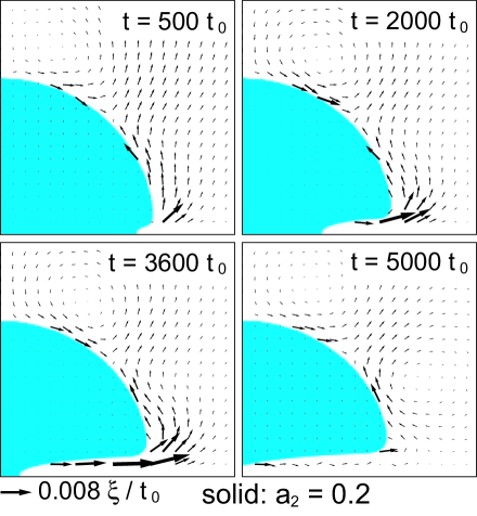
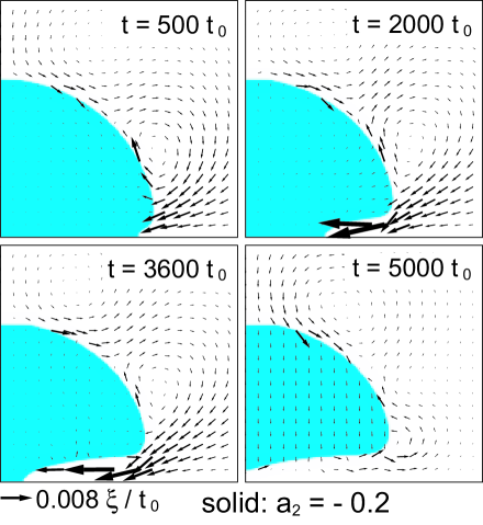
Figure 1: Solid domain at four times on a heated wall for $a_{2}=0.2$ (upper four plates) and for $a_{2}=-0.2$ (lower four plates) in the region $1/2<x/L<7/8$ and $0<y/H<3/4$. Arrows represent the velocity field. Those below the panels correspond to $0.008\xi/t_{0}$. Melting mostly takes place close to the heated wall, where the velocity is from solid to liquid for $a_{2}=0.2$ and from liquid to solid for $a_{2}=-0.2$.

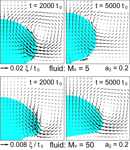
Figure 2: Droplet at liquid-liquid transition with $G=0$ at $t/t_{0}=2000$ and $5000$ on a heated wall in the region $1/2<x/L<7/8$ and $0<y/H<3/4$. The viscosity ratio $M_{v}$ is 5 (top) and 50 (bottom). A typical velocity is $0.02\xi/t_{0}$ for $M_{v}=5$ and $0.008\xi/t_{0}$ for $M_{v}=50$. A circulating velocity field is marked. See Fig.5 for the velocity along the interface.

4 Numerical Method

In two examples to follow, we integrated Eqs. (7), (8), and (11)-(13) in two dimensions on a $800\times 400$ lattice. We use the entropy equation (13) instead of the energy equation (9) to suppress the so-called parasitic flow [15], which is an artificial flow around an interface [17, 18]. The simulation mesh length is $\Delta x=\xi=(C/A)^{1/2}$. Here we set $A=0.4n_{0\ell}k_{B}$, so $C=0.4n_{0\ell}k_{B}\xi^{2}$. The horizontal and vertical lengths of the system are then $L=800\xi$ and $H=400\xi$, respectively. We imposed the periodic boundary condition along the horizontal $x$ axis and the no-slip condition ${\mbox{\boldmath$v$}}={\mbox{\boldmath$0$}}$ at $y=0$ and $H$. In addition, neglecting the surface entropy and energy, we set $\partial\phi/\partial z=0$ at $y=0$ and $H$.

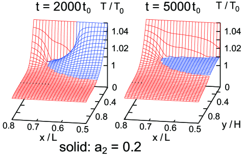
Figure 3: Temperature in the region $0.5<x/L<0.8$ and $0<y/H<1$ for the solid case with $a_{2}=0.2$. See the corresponding domain shapes in Fig.1. At $t=2000t_{0}$ (left), heat from the wall is used to melt the solid near the contact point. At $t=5000t_{0}$ (right), the domain is detached from the wall and its interface temperature becomes a constant.

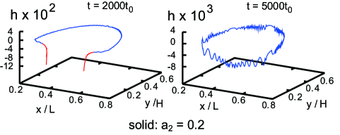
Figure 4: $h$ in Eq.(22) of a melting solid along the interface, which is multiplied by $100$ at $t=2000t_{0}$ (left) and by $1000$ at $t=5000t_{0}$ (right). It represents the distance from the coexistence curve, where $h>0$ in the body part (blue) and $h<0$ in the constricted part (red).

The thermodynamic quantities are given by $C_{p}^{0}=1.1C_{V}^{0}=9.17n_{0\ell}k_{B}$, $K_{T}^{0}=0.064/n_{0\ell}k_{B}T_{0}$, and $\alpha_{p}^{0}=0.20/T_{0}$, which are consistent with the thermodynamic identity $T\alpha_{p}^{2}=(C_{p}-C_{v})K_{T}$ of fluids[11]. The shear modulus is $G=10n_{\ell 0}k_{B}T_{0}\phi^{2}$ for solid-liquid transitions. By setting $a_{1}=-0.27$, we examine two cases of $a_{2}=\Delta n/n_{0\ell}=0.2$ and $-0.2$. The latent heat $q_{0}$ in Eq.(25) is $2.5k_{B}T_{0}$ for $a_{2}=0.2$ and $1.9k_{B}T_{0}$ for $a_{2}=-0.2$.

The viscosities are given by $\eta(\phi)=\eta_{B}(\phi)=\eta_{\ell}+(\eta_{s}-\eta_{\ell})\phi^{2}$. Let $\nu_{0}=\eta_{\ell}/mn_{0\ell}$ be the liquid kinematic viscosity. We measure space and time in units of $\xi$ and

$$t_{0}=0.4\xi^{2}/\nu_{0}.$$ (26)

The viscosity ratio $M_{v}=\eta_{s}/\eta_{\ell}$ is taken to be 10 or 50. The simulation time mesh $\Delta t$ is $0.005t_{0}$ for $M_{v}=10$ and $0.0025t_{0}$ for $M_{v}=50$. The thermal conductivity is $\lambda=1.63\nu_{0}C_{p}^{0}(1+3\phi^{2})$, so the Prandtl number is $1/1.63$ in liquid. The kinetic coefficient for $\phi$ is $\Lambda=0.16/n_{0\ell}k_{B}T_{0}t_{0}$. With these expressions, the reference temperature $T_{0}$ and density $n_{0\ell}$ do not appear in the scaled dynamic equations.

5 A semispheric domain on a heated substrate

First, we placed a solid (type II liquid) semisphere with radius $R=200\xi$ on the substrate in liquid (type I liquid), where $\phi=1$ inside the domain, $\phi=0$ outside it, and $\tau=\zeta=e_{2}=e_{3}=0$ in the whole cell. Thus $T=T_{0}$ and $\delta n=n_{0\ell}a_{2}\theta(\phi)$ were imposed. The boundary temperatures at $z=0$ and $H$ were fixed at $T_{0}$. Then small relaxations followed near the interface in short times ($\sim t_{0}$). After an equilibration time of $100t_{0}$, we raised the bottom temperature to $1.05T_{0}$. We set $t=0$ at this heating.

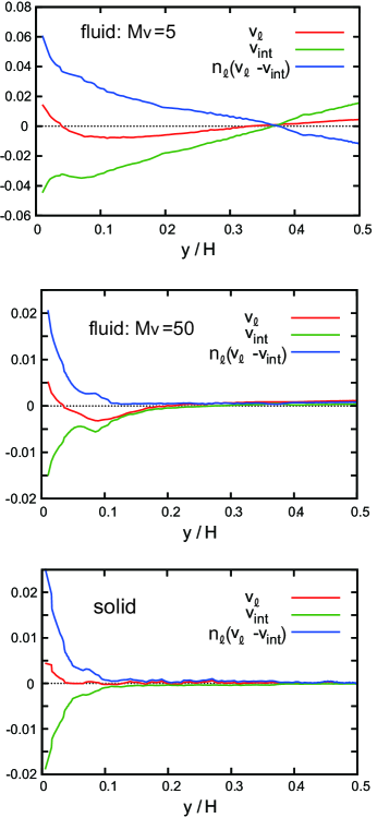
Figure 5: Liquid velocity $v_{\ell}$, interface velocity $v_{int}$, and melting flux $J=n_{\ell}(v_{\ell}-v_{int})$ in the normal direction along the interface in units of $\xi/t_{0}$ or $n_{0\ell}\xi/t_{0}$, where $t=2000t_{0}$ and $a_{2}=0.2$. They are for liquid-liquid transitions with $M_{v}=5$ (top) and 50 (middle) and for a solid-liquid transition (bottom). Melting occurs mostly in the constricted part close to the heated wall.

In Fig.1, we show the domain shapes and the surrounding velocity at four times. The solid density is higher or lower than the liquid density depending on the sign of $a_{2}$. The phase change takes place mostly near the heated wall. For $a_{2}=0.2$ the flow is from the solid to the liquid near the bottom in the upper plates, while for $a_{2}=-0.2$ the flow is in the reverse direction in the lower plates. The solid velocity is very small and is nearly uniform within the domain. The strains $e_{2}$ and $e_{3}$ remain of order $10^{-3}$ and are well in the linear elasticity regime. Nevertheless, the resultant shear stress ($\sim 10^{-2}n_{0\ell}k_{B}T_{0}$) can realize the solid body motion. In addition, the pressure $p$ in the liquid region gradually increases for $a_{2}>0$ and decreases for $a_{2}<0$ due to the density difference. In our examples the deviation $p-p_{0}$ in the liquid is of order $\pm 0.15n_{0\ell}k_{B}T_{0}$ for $a_{2}=\pm 0.2$ at $t=10^{4}t_{0}$. (Here the resultant adiabatic temperature change is very small since $(\partial T/\partial p)_{s}\sim 0.03/n_{0\ell}k_{B}$.)

Figure 2 gives the profiles of a droplet in a less viscous liquid at liquid-liquid transitions with $G=0$. The velocity field decreases with increasing the viscosity ratio $M_{v}=\eta_{s}/\eta_{\ell}$, but it still remains noticeable in the projected part of the domain even for $M_{v}=50$. Here an interface motion induces a fluid motion with a small velocity gradient within a highly viscous droplet. However, the domain shapes in the two cases in Figs.1 and 2 are very similar.

In Fig.3, the temperature is displayed for the solid case with $a_{2}=0.2$ before and after detachment of the domain. Similar profiles were also obtained for the case of liquid-liquid transitions. A steep gradient can be seen near the heated wall, but the interface temperature is nearly flat at the melting temperature $T_{\rm cx}(p)$ far from the wall. Thus the interface is divided into the body part far from the wall and the constricted part close to the wall. In this case the thermal diffusion length $(D_{T}t)^{1/2}\sim(t/t_{0})^{1/2}\xi$ is still shorter than the cell height $H=400\xi$, resulting in a small temperature gradient in the upper region. In Fig.4, we show that $h$ in Eq.(22) is very small on the interface. Here $h\cong-2.5[\tau-(\partial T/\partial p)_{\rm cx}(p-p_{0})/T_{c}]$ away from the interface (or for $\phi=0$ or 1 in Eq.(23)). In the constricted part, the gradient of $h$ is $-10\%$ of that of $\tau$.

In Fig.5, we plot the liquid velocity $v_{\ell}={\mbox{\boldmath$\nu$}}\cdot{\mbox{\boldmath$v$}}$, the interface velocity $v_{int}={\mbox{\boldmath$\nu$}}\cdot{\mbox{\boldmath$v$}}_{int}$, and the melting flux $J=n_{\ell}(v_{\ell}-v_{int})$ through the interface, where $n_{\ell}$ is the liquid density. These are the quantities close to the interface in the normal direction $\nu$. Indeed, melting mostly occurs in the constricted part for large $M_{v}$ and for the solid case. We also notice that $|v_{int}|$ is considerably larger than $|v_{\ell}|$, which is obviously due to the small size of $a_{2}$.

6 A solid domain in a sheared warmer liquid

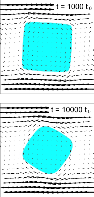
Figure 6: A square-shaped solid domain in a warmer liquid under shear flow with $\dot{\gamma}=2\times 10^{-4}t_{0}^{-1}$ at $\dot{\gamma}t=0.2$ (top) and 2 (bottom). It gradually melts and rotates as a solid body. Melted particles are convected to cool the surrounding liquid.

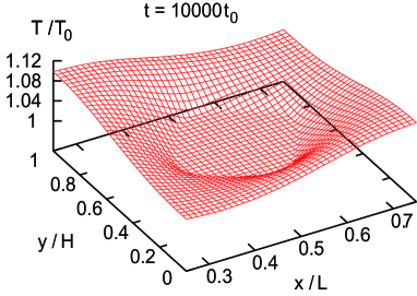
Figure 7: Temperature profile around a melting solid in shear flow at $\dot{\gamma}t=2$, corresponding to the lower panel of Fig.6. It is lowest in the directions making angles of $\pi/4$ and $5\pi/4$ with respect to the $x$ axis due to convection of cooler melted particles.

Next, at $t=0$, we placed a 240$\times$240 solid square with $a_{2}=0.2$ in a liquid. The temperature was initially $0.95T_{0}$ in the solid and $1.1T_{0}$ in the liquid. The top and bottom plates were insulating or $\partial T/\partial z=0$. By moving them we applied a shear flow with rate $\dot{\gamma}=2\times 10^{-4}t_{0}^{-1}$ for $t>0$. The liquid should be cooled upon melting.

Figure 6 displays the solid shapes at $t=10^{3}t_{0}=0.2/\dot{\gamma}$ and $10^{4}t_{0}=2/\dot{\gamma}$ in the middle region $1/4<x/L<3/4$ and $0<y/H<1$, where the solid is rotating and melting. The final solid area in Fig.6 is $70\%$ of the initial area. Figure 7 gives the temperature profile at $t=10^{4}t_{0}$. It demonstrates a considerable cooling of the liquid particularly in the regions where the melted liquid has been convected. The temperature is homogeneous with $h\cong 0$ within the solid domain. The average temperature $\langle{T}\rangle=\int_{0}^{L}dx\int_{0}^{H}dyT({\mbox{\boldmath$r$}},t)/LH$ is $1.078T_{0}$ at $t=0$, $1.076T_{0}$ at $t=10^{3}t_{0}$, and $1.063T_{0}$ at $t=10^{4}t_{0}$. To explain the cooling by $0.015T_{0}$ at $t=10^{4}t_{0}$, we multiply the number of melted particles ($\sim 4000$) by the latent heat per particle $q_{0}$ in Eq.(25) and divide it by the total specific heat $LHC_{v}^{0}$ to obtain a temperature decrease $\sim 0.015T_{0}$ in accord with the data of $\langle{T}\rangle$.

7 Summary

In our theory, the entropy depends on the phase field $\phi$ and contains a gradient part ($\propto|\nabla\phi|^{2}$), while the total energy consists of the usual internal energy, the kinetic energy, and the elastic energy. The elasticity is introduced using strain fields $e_{2}$ and $e_{3}$ in two dimensions, which represent anisotropic elastic deformations. Starting with these quantities and using the principle of nonnegative entropy production, we have constructed dynamic equations for the phase field, the hydrodynamic variables, and the strains. They can describe phase transition dynamics accounting for the hydrodynamic and elastic effects. If the strains are absent or the shear modulus vanishes, we obtain the dynamic equations applicable to liquid-liquid phase transitions. We have also proposed to use the entropy density containing second-order deviations of the number and internal energy densities from a reference two-phase state. We have solved the dynamic equations to examine two melting phenomena in two dimensions. In these cases small strains of order $10^{-3}$ have produced rigid body motions of a solid domain.

There can be a number of problems to be studied in our scheme such as dendrite formation in flow, spinodal decomposition, epitaxial growth, and recrystallization. In particular, it is of great interest to investigate kinetics with large strains or even with dislocations. In liquid-liquid transitions, we should further investigate the effects of latent heat and shear flow in phase ordering.

- [1] \NameLanger J.S. \REVIEW Rev. Mod. Phys.5219801
- [2] \NameGlicksman M.E., Coriell S.R., and McFadden G.B. \REVIEW Ann. Rev. Fluid Mech. 181986 307
- [3] \NameKobayashi R. \REVIEW Physica D631993410.
- [4] \NameKarma A. and Rappel W.-J. \REVIEW Phys. Rev. E5719984323
- [5] \NameTnhardt R. and Amberg G. \REVIEW J. of Crys. Growth 1941998 406
- [6] \NameBeckermann C., Diepers H.-J., Steinbach I., Karma A., and Tong X. \REVIEW J. Comput. Phys.1541999 468
- [7] \NameAnderson D.M., McFadden G.B., and Wheeler A.A. \REVIEW Physica D 1352000 175
- [8] \NameJeong J.-H., Goldenfeld N., and Dantzig J.A. \REVIEW Phys. Rev. E 642001 041602
- [9] \Name Mller J. and Grant M. \REVIEW Phys. Rev. Lett. 8219991736
- [10] \NameKassener K. and Misbah C. \REVIEW Europhys. Lett. 461999 217
- [11] \NameOnuki A. Phase Transition Dynamics (Cambridge University Press, Cambridge, 2002).
- [12] \NameKatayama Y. et al. \REVIEW Nature 403170 2000.
- [13] \NameR. Kurita and H. Tanaka \REVIEW J. Chem. Phys. 1262007204505
- [14] \NameOnuki A. \REVIEW Phys. Rev. E752007036304
- [15] \NameTeshigawara R. and Onuki A. \REVIEWEurophys. Lett. 84200836003
- [16] \NameOnuki A. \REVIEW Phys. Rev. E 682003 061502
- [17] \NameJamet D., Torres D., and Brackbill J. U. \REVIEW J. Comput. Phys. 1822002262
- [18] \NameShin S., Abdel-Khalik S. I., Daru V., and Juric D. \REVIEW J. Comput. Phys. 2032005 493