Coupled inflaton and electromagnetic fields from Gravitoelectromagnetic Inflation with Lorentz and Feynman gauges.

Abstract:

Using a semiclassical approach to Gravitoelectromagnetic Inflation (GEMI), we study the origin and evolution of seminal inflaton and electromagnetic fields in the early inflationary universe from a 5D vacuum state. We use simultaneously the Lorentz and Feynman gauges. Our formalism is naturally not conformal invariant on the effective 4D de Sitter metric, which make possible the super adiabatic amplification of electric and magnetic field modes during the early inflationary epoch of the universe on cosmological scales. This is the first time that solutions for the electric field fluctuations are investigated in a systematic way as embeddings for inflationary models in 4D. An important and new result here obtained is that the spectrum of the electric field fluctuations depend with the scale, such that the spectral index increases quadratically as the scale decreases.

1 Introduction

The origin of cosmological scales magnetic fields is one of the most important, fascinating and challenging problems in modern cosmology. Many scenarios have been proposed to explain them. Magnetic fields are known to be present on various scales of the universe[1]. Primordial large-scale magnetic fields may be present and serve as seeds for the magnetic fields in galaxies and clusters.

Until recently the most accepted idea for the formation of large-scale magnetic fields was the exponentiation of a seed field as suggested by Zeldovich and collaborators long time ago. This seed mechanism is known as galactic dynamo. However, recent observations have cast serious doubts on this possibility. There are many reasons to believe that this mechanism cannot be universal. This is why the mechanism responsible for the origin of large-scale magnetic fields is looked in the early universe, more precisely during inflation[2], which should be amplified through the dynamo mechanism after galaxy formation. In principle, one should be able to follow the evolution of magnetic fields from their creation as seed fields through to dynamo phase characteristic of galaxies. It is believed that magnetic fields can play an important role in the formation and evolution of galaxies and their clusters, but are probably not essential to our understanding of large-scale structure in the universe. However, an understanding of structure formation is paramount to the problem of galactic and extragalactic magnetic fields[3, 4].

It is natural to look for the possibility of generating large-scales magnetic fields during inflation with strength according with observational data on cosmological scales: $<10^{-9}$ Gauss[5]. However, the FRW universe is conformal flat and the Maxwell theory is conformal invariant, so that magnetic fields generated at inflation would come vanishingly small at the end of the inflationary epoch. The possibility to solve this problem relies in produce non-trivial magnetic fields in which conformal invariance to be broken.

On the other hand, the five dimensional model is the simplest extension of General Relativity (GR), and is widely regarded as the low-energy limit of models with higher dimensions (such as 10D supersymmetry and 11D supergravity). Modern versions of 5D GR abandon the cylinder and compactification conditions used in original Kaluza-Klein (KK) theories, which caused problems with the cosmological constant and the masses of particles, and consider a large extra dimension. In particular, the Induced Matter Theory (IMT) is based on the assumption that ordinary matter and physical fields that we can observe in our 4D universe can be geometrically induced from a 5D Ricci-flat metric with a space-like noncompact extra dimension on which we define a physical 5D apparent vacuum. The vacuum we shall consider is very restrictive in the sense that we shall not consider any kind of charges, matter or currents on the 5D spacetime. In a relativistic framework, it can be expressed by the 5D null geodesic equations, which are only valid for massless test particles in 5D. However, observers that move with frames $U^{4}\equiv{dx^{4}\over dS}=0$ (described by a constant foliation on the extra dimension), can see the physics described by the effective 4D energy-momentum tensor embedded in the 5D apparent vacuum, which is geometrically described by a 5D Ricci-flat spacetime. From the mathematical point of view, the Campbell-Magaard theorem[6] serves as a ladder to go between manifolds whose dimensionality differs by one. This theorem, which is valid in any number of dimensions, implies that every solution of the 4D Einstein equations with arbitrary energy-momentum tensor can be embedded, at least locally, in a solution of the 5D Einstein field equations in vacuum. Because of this, matter, charge and currents may be 4D manifestations of the topology of space.

Gravitoelectromagnetic Inflation (GEMI)[7] was proposed recently with the aim to describe, in an unified manner, electromagnetic, gravitational and the inflaton fields in the early inflationary universe, from a 5D vacuum. It is known that conformal invariance must be broken to generate non-trivial magnetic fields. A very important fact is that in this formalism conformal invariance is naturally broken. Other conformal symmetry breaking mechanisms have been proposed so far[8]. However, most of these are developed in the Coulomb gauge. In order to simplify the equations of motion for $A^{\nu}$, in this paper we use simultaneously the Lorentz and Feynman gauges, to calculate the electric and magnetic spectral indices for the spectrums of these fluctuations taking into account the induced currents. The main contribution of this paper is the study for the spectrum of the electric field fluctuations in a systematic way as embeddings for inflationary models in 4D. This topic has been ignored in the literature.

The paper is organized as follows: in Sect. II we introduce the 5D vacuum of the fields on a generic 5D Ricci flat metric, to obtain the equations for the vector fields using simultaneously the generalized Lorentz and Feynman gauges. Also, we impose a semiclassical approach to the vector fields. In Sect. III we study the particular case of a 5D Ricci flat space-time for an extended de Sitter expansion. In Sect. IV describe the dynamics of the vector fields on an effective 4D de Sitter space-time, when we make a static foliation on the noncompact extra dimension, which is considered as space-like: $\psi=\psi_{0}$. We develop the equations of motion for the fields using a particular Lorentz gauge on the effective 4D de Sitter space-time. After it, we describe the dynamics of the classical and quantum fields, to finally calculate the evolution and spectrums of the inflaton, electric and magnetic fields. The conclusions are developed in the Sect. V. Finally, we have included two appendixes where we have developed respectively the details of the calculations for the modes of the electric field fluctuations, and the spectrum for these fluctuations.

2 Vector fields in 5D vacuum

We begin considering a 5D manifold $\cal{M}$ described by a symmetric $g_{ab}=g_{ba}$ 5D tensor metric. This manifold $\cal M$ is mapped by coordinates $\{x^{a}\}$

$$dS^{2}=g_{ab}dx^{a}dx^{b}.$$ (1)

From the geometrical point of view, to describe a relativistic 5D vacuum, we shall consider that $g_{ab}$ is such that the Ricci tensor $R_{ab}=0$, and hence: $G_{ab}=0$. To describe the system we introduce the action on the manifold $\cal M$

$$\mathcal{S}=\int d^{5}x\sqrt{-g}\left[\frac{{}^{(5)}\,R}{16\pi G}-\frac{1}{4}Q_{bc}Q^{bc}\right],$$ (2)

where ${}^{(5)}\,R$ is the 5D scalar curvature on the five-dimensional metric (1) and $Q^{ab}=F^{ab}-\gamma g^{ab}\nabla_{f}A^{f}$, where the 5D Faraday tensor is $F^{bc}=\nabla^{b}A^{c}-\nabla^{c}A^{b}=\partial^{b}A^{c}-\partial^{c}A^{b}$. We shall consider that the fields $A^{b}$ are minimally coupled to gravity and free of interactions, so that the second term in the action is purely kinetic.

2.1 Einstein Equations in 5D

If we minimize the action respect to the metric we will obtain Einstein Equations in 5D. In this paper we shall use a semiclassical approach where the Einstein equations are expressed by the homogeneous component of the fields. This slightly differs from the one used by [9] in the fact that we don’t need to renormalize the stress tensor, but at the cost of assuming a semiclassical behavior of the fields that rules out the dependence with the wavenumber in the calculation of the semiclassical Einstein equations

$$G_{ab}=-8\pi G\,T^{(0)}_{ab},$$ (3)

where $T^{(0)}_{ab}\equiv\langle T_{ab}(\bar{A}^{c})\rangle$. Notice that we use a semiclassical expansion of the vector fields

$$A^{c}=\bar{A}^{c}+\delta A^{c},$$ (4)

where the overbar symbolizes the 3D spatially homogeneous background field consistent with the fixed homogeneous metric and $\delta A^{c}$ describes the fluctuations with respect to $\bar{A}^{c}$. In this sense when we perform the expectation value of the stress tensor, adopting the ansatz $\langle\delta A_{c}\rangle=0$, only will appear zero order $T^{(0)}_{ab}$ and the second order $T^{(2)}_{ab}$ in perturbations terms. The last corresponds to a feedback term and is related to back-reaction effects, which do not will be consider in this paper. The stress tensor is defined by the fields lagrangian being symmetric by definition

$$T_{bc}=\frac{2}{\sqrt{g}}\left\{\frac{\partial}{\partial g^{bc}}\left(\sqrt{g}{\cal L}_{f}\right)-\frac{\partial}{\partial x^{e}}\left[\frac{\partial}{\partial{g^{bc}}_{,\,e}}\left(\sqrt{g}{\cal L}_{f}\right)\right]\right\}.$$ (5)

The appearance of variations with respect to derivatives of the metric is because we are dealing with vector fields whose covariant derivative operators involve Christoffel symbols (i.e. ordinary derivatives of the metric). In our case the stress tensor reduces to

$$T_{bc} = {F^{e}}_{b}F_{ce}+\frac{1}{4}g_{bc}F_{de}F^{de}-\lambda\left\{2{A^{e}}_{;\,e}\left[A_{(b;\,c)}-\left(2A_{(b}g_{c)h,\,f}+g_{hf,\,(b}A_{a)}\right)g^{hf}\right]+\right.$$

$$+ \left.g_{bc}\left[\left(A^{e}_{,\,ef}+\Gamma^{e}_{de,\,f}A^{d}+\Gamma^{e}_{de}A^{d}_{,\,f}+2\Gamma^{e}_{ef}A^{d}_{,\,d}+\frac{3}{2}\Gamma^{e}_{ed}\Gamma^{a}_{af}A^{d}\right)A^{f}+\frac{1}{2}\left(A^{e}_{,\,e}\right)^{2}\right]\right.$$

$$+ \left.g_{bc,\,f}A^{f}A^{e}_{;\,c}\right\},$$ (7)

where $\gamma^{2}=\frac{2\lambda}{5}$.

2.2 5D dynamics of the fields

The Euler-Lagrange equations give us the dynamics for $A_{b}$

$$\nabla_{f}\nabla^{f}A^{b}-R_{f}^{b}A^{f}-(1-\lambda)\nabla^{b}\nabla_{f}A^{f}=0.$$ (8)

In particular, the choice $\lambda=1$ is known as Feynman gauge, somehow equivalent to a Lorentz gauge $\nabla_{f}A^{f}=0$. In this paper we shall choose simultaneously both conditions. The first one assures that the balance of each component of any external current to be null, and the second one is more restrictive, because assures that each direction (insider or outsider) of each component of the current to be zero.

It is easy to show that the 5-divergence of the field equation of motions satisfy the same equation as in a Minkowski space, but changing ordinary partial derivatives by the covariant derivative

$$\nabla^{a}\nabla_{a}\left(\nabla_{f}A^{f}\right)=0.$$ (9)

Hence, the Lorentz gauge is satisfied for appropriate initial conditions of $\nabla_{a}A^{a}=0$. With such a choice the field lagrangian density ${\cal L}_{f}=-\frac{1}{4}Q^{2}$ is

$${\cal L}^{\prime}_{f}=-\frac{1}{2}\nabla_{a}A_{b}\nabla^{a}A^{b}=-\frac{1}{2}\nabla_{\mu}A_{\nu}\nabla^{\mu}A^{\nu}-\frac{1}{2}\nabla_{4}A_{\nu}\nabla^{4}A^{\nu}-\frac{1}{2}\nabla_{\mu}A_{4}\nabla^{\mu}A^{4}-\frac{1}{2}\nabla_{4}A_{4}\nabla^{4}A^{4},$$ (10)

where $Q^{2}=Q^{ab}Q_{ab}$. For 4D observers living in a hypersurface where the fifth component of the vector field is normal to it, this extra dimensional field will manifest separately, like an effective 4D vector field $A^{\nu}$ and a 4D scalar field $A^{4}$. In this sense we can identify kinetic terms for both, scalar and vector fields, and the derivatives with respect to the extra dimension may be interpreted as potential (or dynamical sources) terms joined with massive terms for each of them.

The stress tensor in this gauge is

$$T_{ab}= -\nabla_{a}A_{e}\nabla_{b}A^{e}-\nabla_{e}A_{a}\nabla^{e}A_{b}-2g_{c(b}A_{a)}\Gamma^{c}_{ef}\nabla^{e}A^{f}+\frac{1}{2}g_{ab}\nabla_{e}A_{f}\nabla^{e}A^{f}-$$

$$2\frac{g_{,f}}{g}\left[\nabla_{(a}A_{b)}A^{f}+\nabla^{f}A_{(b}A_{a)}-A_{(a}\nabla_{b)}A^{f}\right]-\left[\nabla_{(a}A_{b)}A^{f}+\nabla^{f}A_{(b}A_{a)}-A_{(a}\nabla_{b)}A^{f}\right]_{,f}.$$

3 Special case: 5D generalization of a de Sitter spacetime

Because we are interested to study a cosmological scenario of inflation from the context of the theory of Space-Time-Matter, we shall consider the 5D Riemann-flat metric[10]

$$dS^{2}=\psi^{2}dN^{2}-\psi^{2}e^{2N}dr^{2}-d\psi^{2},$$ (12)

where $N$ is a time-like dimension related to the number of e-folds, $dr^{2}=dx^{i}\delta_{ij}dx^{j}$ is the Euclidean line element in cartesian coordinates and $\psi$ is the space-like extra dimension. This metric satisfies the vacuum condition $G^{ab}=0$.

For this 5D metric the field equations, after taking Lorentz gauge: $\nabla_{a}A^{a}=\partial_{N}A^{0}+3A^{0}+\partial_{\psi}A^{4}+4\psi^{-1}A^{4}+\partial_{i}A^{i}=0$, are

$$\left\{\frac{\partial^{2}}{\partial N^{2}}+5\frac{\partial}{\partial N}-e^{-2N}\partial^{2}_{r}-\psi^{2}\left[\frac{\partial^{2}}{\partial\psi^{2}}+\frac{6}{\psi}\frac{\partial}{\partial\psi}\right]\right\}{A^{0}}+\left[\frac{2}{\psi}\frac{\partial}{\partial N}+2\frac{\partial}{\partial\psi}+\frac{8}{\psi}\right]\,{A^{4}}=0,$$ (13)

$$\left\{\frac{\partial^{2}}{\partial N^{2}}+5\frac{\partial}{\partial N}-e^{-2N}\partial^{2}_{r}-\psi^{2}\left[\frac{\partial^{2}}{\partial\psi^{2}}+\frac{6}{\psi}\frac{\partial}{\partial\psi}\right]\right\}{A^{j}}-2\partial^{j}\left(A^{0}+\frac{A^{4}}{\psi}\right)=0,$$ (14)

$$\left\{\frac{\partial^{2}}{\partial N^{2}}+3\frac{\partial}{\partial N}-e^{-2N}\partial^{2}_{r}-\psi^{2}\left[\frac{\partial^{2}}{\partial\psi^{2}}+\frac{6}{\psi}\frac{\partial}{\partial\psi}+\frac{12}{\psi^{2}}\right]\right\}{A^{4}}=0.$$ (15)

Notice that the (15) is decoupled after applying the Lorentz gauge. However we see that it is not sufficient to decouple all the field equations. This is because the non zero connections of the metric (12) act in a non trivial manner in the vector fields derivatives. There are 14 non zero Christoffel symbols

$$\Gamma^{\mu}_{\mu 4}=\psi^{-1},\ \ \Gamma^{i}_{i0}=1,\ \ \Gamma^{0}_{ii}=e^{2N},\ \ \Gamma^{4}_{00}=\psi,\ \ \Gamma^{4}_{ii}=-\psi e^{2N}.$$ (16)

Therefore, in this Riemann-flat spacetime we obtain the D ’Alambertian of the $A^{b}$ field

$$\nabla_{f}\nabla^{f}A^{b}=0,$$ (17)

but, expressed in terms of the ordinary derivatives and the Christoffel symbols we notice the coupling terms

$$g^{fh}\left\{\partial_{f}\partial_{h}A^{b}+2\Gamma^{b}_{ef}\partial_{h}A^{e}+\Gamma^{b}_{he,\,f}A^{e}-\Gamma^{e}_{fh}\partial_{e}A^{b}-\Gamma^{e}_{fh}\Gamma^{b}_{ed}A^{d}+\Gamma^{b}_{ef}\Gamma^{e}_{hd}A^{d}\right\}=0.$$ (18)

Notice that in a 5D Minkowskian metric: $dS^{2}=dt^{2}-dr^{2}-d\psi^{2}$, the connections vanish and the field equations remain decoupled after the gauge choice.

3.1 Dynamics of the 3D spatially isotropic background fields

We shall combine the field equations of motion for the classical homogeneous fields with the Einstein Equations, the first ones reduce to

$$\left\{\frac{\partial^{2}}{\partial N^{2}}+5\frac{\partial}{\partial N}-\psi^{2}\left[\frac{\partial^{2}}{\partial\psi^{2}}+\frac{6}{\psi}\frac{\partial}{\partial\psi}\right]\right\} {\bar{A}^{0}} +\left[\frac{2}{\psi}\frac{\partial}{\partial N}+2\frac{\partial}{\partial\psi}+\frac{8}{\psi}\right]\,{\bar{A}^{4}}=0,$$ (19)

$$\left\{\frac{\partial^{2}}{\partial N^{2}}+5\frac{\partial}{\partial N}-\psi^{2}\left[\frac{\partial^{2}}{\partial\psi^{2}}+\frac{6}{\psi}\frac{\partial}{\partial\psi}\right]\right\} {\bar{A}^{j}} =0,$$ (20)

$$\left\{\frac{\partial^{2}}{\partial N^{2}}+3\frac{\partial}{\partial N}-\psi^{2}\left[\frac{\partial^{2}}{\partial\psi^{2}}+\frac{6}{\psi}\frac{\partial}{\partial\psi}+\frac{12}{\psi^{2}}\right]\right\} {\bar{A}^{4}} =0.$$ (21)

Notice that the equation for $\bar{A}^{0}$ is the unique coupled. Furthermore, once obtained ${\bar{A}^{4}}$, we can describe the dynamics of ${\bar{A}^{0}}$ in (19), where ${\bar{A}^{4}}$ appears as a source.

4 Effective 4D dynamics of the fields

Now we consider a static foliation on the 5D metric (12). The resulting 4D hypersurface after making $\psi=\psi_{0}$ describes a de Sitter spacetime. From the relativistic point of view an observer moving with the penta velocity $U_{\psi}=0$, will be moving on a spacetime that describes a de Sitter expansion which has a scalar curvature ${}^{(4)}R=12/\psi^{2}_{0}=12\,H^{2}_{0}$, such that the Hubble parameter is defined by the foliation $H_{0}=\psi_{0}^{-1}$. Hence, if we consider the coordinate transformations on (12)

$$t=\psi_{0}N,\ \ \ R=\psi_{0}r,\ \ \ \psi=\psi,$$ (22)

we then arrive to the Ponce Leon metric[11]: $dS^{2}=\left(\frac{\psi}{\psi_{0}}\right)^{2}\left[dt^{2}-e^{2t/\psi_{0}}dR^{2}\right]-d\psi^{2}$. If we foliate $\psi=\psi_{0}$, we get the effective 4D metric

$$dS^{2}\rightarrow ds^{2}=dt^{2}-e^{2H_{0}t}d\vec{R}^{2},$$ (23)

which describes a 3D spatially flat, isotropic and homogeneous de Sitter expanding universe with a constant Hubble parameter $H_{0}$.

The dynamics of the fields being given by the equations (13), (14) and (15), evaluated on the foliation $\psi=\psi_{0}=1/H_{0}$, with the transformations (22). In the following subsections we shall study separately the dynamics of the classical 3D spatially isotropic fields: $\bar{A}^{\mu}(t,\psi_{0})$ and $\bar{A}^{4}(t,\psi_{0})$, and the fluctuations of these fields: $\delta A^{\mu}(t,\vec{R},\psi_{0})$ and $\delta A^{4}(t,\vec{R},\psi_{0})$. Notice that now $\vec{R}\equiv\vec{R}(X^{i})$. To describe the dynamics of the fields we shall impose the effective 4D Lorentz gauge: ${}^{(4)}\nabla_{\mu}A^{\mu}=0$. It implies that the 5D Lorentz gauge with the transformations (22) and evaluated on the foliation must now be

$$\left.\nabla_{a}A^{a}\right|_{\psi_{0}}=^{(4)}\nabla_{\mu}A^{\mu}(t,\vec{R},\psi_{0})+\left.\left(\partial_{\psi}A^{4}+4\psi^{-1}A^{4}\right)\right|_{\psi_{0}}=0,$$ (24)

where ${}^{(4)}\nabla_{\mu}\,A^{\mu}$ denotes the covariant derivative on the effective 4D metric (23). Hence, in order to the effective 4D Lorentz gauge to be fulfilled, we shall require

$$\left.\left(\partial_{\psi}A^{4}+4\psi^{-1}A^{4}\right)\right|_{\psi_{0}}=0.$$ (25)

4.1 4D classical field dynamics

In order to solve the equations (19), (20) and (21) on an effective 4D de Sitter metric, we must evaluate these equations on the particular foliation $\psi=\psi_{0}=H^{-1}_{0}$, $r=R\,\psi_{0}$ and $N=H_{0}\,t$. We shall identify the effective scalar $A^{4}$ with the inflaton field: $A^{4}(t,\vec{R},\psi_{0})\equiv\phi(t,\vec{R},\psi_{0})$ and we shall denote $\bar{\phi}(t,\psi_{0})\sim\left.\phi_{1}(N)\,\phi_{2}(\psi)\right|_{N=H_{0}t,\psi=\psi_{0}=H^{-1}_{0}}$, as the 3D spatially isotropic and homogeneous background field. In the same way we state for the homogeneous component of the vector field the separation $\bar{A}^{j}(t,\psi_{0})\sim\left.S^{j}_{1}(N)S^{j}_{2}(\psi)\right|_{N=H_{0}t,\psi=\psi_{0}=H^{-1}_{0}}$, in the next we shall drop the index $j$ to label the functions $S_{1}(t)$ and $S_{2}(\psi_{0})$. Hence, we obtain

$$\bar{\phi}(t,\psi_{0})=e^{-\frac{3}{2}H_{0}t}\left(a_{1}\,e^{\alpha H_{0}t}+a_{2}\,e^{-\alpha H_{0}t}\right),\ \ \ \ \alpha=\frac{3}{2}\sqrt{1-\frac{4m^{2}}{9}},$$ (26)

where we have considered the condition (25), such that

$$\left.-\psi^{2}\left[\frac{\partial^{2}}{\partial\psi^{2}}+\frac{3}{\psi}\frac{\partial}{\partial\psi}\right]\bar{A}^{4}\right|_{\psi_{0}}=m^{2}\,\bar{\phi}(t,\psi_{0}),$$ (27)

where $\bar{\phi}$ plays the role of the background inflaton field. Furthermore, the general solution of eq. (20) on the effective 4D metric (23), is

$$\bar{A}^{j}(t,\psi_{0})\sim S(t)=e^{-\frac{5}{2}H_{0}t}\left(c_{1}\,e^{\sigma H_{0}t}+c_{2}\,e^{-\sigma H_{0}t}\right),\ \ \ \ \sigma=\frac{5}{2}\sqrt{1-\frac{4\nu^{2}}{25}}$$ (28)

where

$$\left.-\psi^{2}\left[\frac{\partial^{2}}{\partial\psi^{2}}+\frac{6}{\psi}\frac{\partial}{\partial\psi}\right]\bar{A}^{j}\right|_{\psi_{0}}=\nu^{2}\,\bar{A}^{j}(t,\psi_{0}).$$ (29)

A similar treatment can be done for $\bar{A}^{0}$, after making use of the condition (25), the transformations (22) and the foliation $\psi=\psi_{0}=1/H_{0}$. However, the difference with the other background components of the field observed in eq. (19) is that $\bar{A}^{4}\equiv\bar{\phi}(t,\psi_{0})$ acts as a source of $\bar{A}^{0}(t,\psi_{0})$.

As a particular choice we shall consider a 4D inflationary universe, where the background fields are $\bar{A}^{b}=\left(0,0,0,0,\bar{\phi}\right)$, in agreement with a global (de Sitter) accelerated expansion which is 3D spatially isotropic, flat and homogeneous. . In this case, the relevant components of the classical Energy momentum tensor, are

$$\rho\equiv\langle T^{0}_{0}\rangle = \frac{1}{2}\dot{\bar{\phi}}^{2}+\left[\frac{5}{\psi^{2}}\bar{\phi}^{2}+\frac{1}{2}\bar{\phi}^{\prime 2}+\frac{2}{\psi}\bar{\phi}\bar{\phi}^{\prime}\right]_{\psi=\psi_{0}},$$ (30)

$$p\equiv\langle-T^{i}_{j}\rangle|_{i=j} = \frac{1}{2}\dot{\bar{\phi}}^{2}-\left[\frac{5}{\psi^{2}}\bar{\phi}^{2}+\frac{1}{2}\bar{\phi}^{\prime 2}+\frac{2}{\psi}\bar{\phi}\bar{\phi}^{\prime}\right]_{\psi=\psi_{0}},$$ (31)

$$\langle T^{\alpha}_{\beta}\rangle|_{\alpha\neq\beta} = 0,$$ (32)

where the prime denotes the partial derivative with respect to $\psi$ and dots denote partial derivatives with respect to the time, which in our case are zero: $\left.\dot{\bar{\phi}}\right|_{\psi_{0}}=0$. Furthermore, from eq. (30) we can make the following identification for the background scalar potential:

$$V[\bar{\phi}]=\left[\frac{5}{\psi^{2}}\bar{\phi}^{2}+\frac{1}{2}\bar{\phi}^{\prime 2}+\frac{2}{\psi}\bar{\phi}\bar{\phi}^{\prime}\right]_{\psi=\psi_{0}}.$$ (33)

In our model, the hypersurface $\psi=\psi_{0}$ defines a de Sitter expansion of the universe with a Hubble parameter $H_{0}=\psi_{0}^{-1}$. The equation of state for this case is $p=-\rho=-3/\left(8\pi G\psi^{2}_{0}\right)$. Then, it is easy to see that the only compatible background solution for the field evaluated on the hypersurface is the typical de Sitter solution for a background scalar field: $\bar{\phi}(t=N/H_{0},\psi_{0})=\bar{\phi}_{0}$. This means that

$$V\left[\bar{\phi}(t,\psi_{0})\right]=\frac{3H^{2}_{0}}{8\pi G}.$$ (34)

A particular solution of (25) is

$$\bar{\phi}=\bar{\phi}_{0}\left(\frac{\psi_{0}}{\psi}\right)^{4},\qquad\rightarrow\bar{\phi}^{\prime}\equiv\left.\frac{\partial\bar{\phi}}{\partial\psi}\right|_{\psi=\psi_{0}=1/H_{0}}=-4H_{0}\bar{\phi}_{0}.$$ (35)

From eqs. (33), (34) and the second in (35), we obtain

$$\left.\left(\bar{\phi}\right)^{2}\right|_{\psi=\psi_{0}=1/H_{0}}=\bar{\phi}^{2}_{0}=\frac{3}{40\,\pi\,G},$$ (36)

such that replacing (36) in the second equation of (35), we obtain

$$(\bar{\phi}^{\prime})^{2}\equiv\left(\left.\frac{\partial\bar{\phi}}{\partial\psi}\right|_{\psi=\psi_{0}=1/H_{0}}\right)^{2}=\frac{6H^{2}_{0}}{5\pi G}.$$ (37)

It is easy to see by inspection in (19) that $\bar{\phi}(t,\psi)$ is a constant of $N$. In other words, the unique origin of the effective 4D potential energy density (34) related to the background inflaton field is the $\psi$-dependence of $\bar{\phi}(N,\psi)$.

4.2 4D Field fluctuations

Here we consider equations (13), (14) and (15) to search for possible electromagnetic fields generated through this model. In Sect. (4.1) we’ve seen that the Einstein equations for the background fields exclude any possibility of spatially homogeneous electromagnetic fields.

The equation for the effective scalar $\delta A^{4}(t,\vec{R},\psi_{0})$ on the effective hypersurface (23) is decoupled from the dynamics of the 4-vector. In contrast, the equations for $\delta A^{0}(t,\vec{R},\psi_{0})$ and $\delta A^{i}(t,\vec{R},\psi_{0})$ remain coupled. By the use of our 5D Lorentz gauge evaluated on the foliation $\psi=\psi_{0}=H^{-1}_{0}$: $\left.\nabla_{a}\,A^{a}\right|_{\psi_{0}=H^{-1}_{0}}=0$, we can express the inhomogeneous term for $\delta A^{0}$ as only a function of $\delta A^{4}$. The solution will involve both, homogeneous and inhomogeneous parts. Once obtained $\delta A^{0}$ and $\delta A^{4}$, we can finally search solutions for the components $\delta A^{j}$. These total solutions are necessary to deduce the effective electric fields. In contrast, as we previously said, the equation of motion for pure magnetic fields may be obtained by just applying the curl in the 3-space to equation (14). The last term in (14) vanishes because is a 3-gradient, and so magnetic fields equations are decoupled. To quantize the field fluctuations on the effective 4D de Sitter spacetime (23), we shall consider the equations (13), (14) and (15), with condition (25), the transformations (22) and the foliation $\psi=\psi_{0}=1/H_{0}$. The equal time canonical relations are

$$\left.\left[\delta A_{i}(t,\vec{R},\psi_{0}),\Pi^{j}(t,\vec{R^{\prime}},\psi_{0})\right]\right|_{\psi_{0}=1/H_{0}}=-i\,g^{j}_{i}e^{-3H_{0}t}\,\delta^{(3)}(\vec{R}-\vec{R^{\prime}}),$$ (38)

where $g^{ij}$ are the space-like components of the tensor metric in (23) and $\delta^{(3)}(\vec{R}-\vec{R^{\prime}})$ is the 3D Dirac’s function. Furthermore, the canonical momentum is given by the electric field $\Pi^{j}\equiv E^{j}=\nabla^{j}A^{0}-\nabla^{0}A^{j}$. The equations (13), (14) and (15) with the transformations (22) can be evaluated on the foliation $\psi=\psi_{0}=1/H_{0}$ to give the dynamics on the effective 4D spacetime (23). If we take into account the conditions (25), the effective 4D dynamics of the fluctuations describe an effective 4D Lorentz gauge, so that

$$\frac{\partial^{2}\delta A^{0}}{\partial t^{2}}+5H_{0}\frac{\partial\delta A^{0}}{\partial t}-H^{2}_{0}e^{-2H_{0}t}\partial^{2}_{R}\delta A^{0}+\nu^{2}H^{2}_{0}\delta A^{0}=-2H^{2}_{0}\frac{\partial\delta\phi}{\partial t},$$ (39)

$$\frac{\partial^{2}\delta A^{j}}{\partial t^{2}}+5H_{0}\frac{\partial\delta A^{j}}{\partial t}-H^{2}_{0}e^{-2H_{0}t}\partial^{2}_{R}\delta A^{j}+\nu^{2}H^{2}_{0}\delta A^{j}=2H^{2}_{0}\partial^{j}\left(\delta A^{0}+H_{0}\delta\phi\right),$$ (40)

$$\frac{\partial^{2}\delta\phi}{\partial t^{2}}+3H_{0}\frac{\partial\delta\phi}{\partial t}-H^{2}_{0}e^{-2H_{0}t}\partial^{2}_{R}\delta\phi+m^{2}H^{2}_{0}\delta\phi=0.$$ (41)

describe the 4D dynamics of the fluctuations. A very important fact is that the electromagnetic field fluctuations $\delta A^{\mu}$ obey a Proca equation with sources.

The expansion of the free field in temporal modes is

$$\delta A^{\mu}(t,\vec{R},\psi_{0})=\int\frac{d^{3}K}{(2\pi)^{3}}\sum_{\lambda=1}^{3}\varepsilon^{\mu}(\vec{K},\lambda)\left(a_{(\vec{K},\lambda)}e^{-i\vec{K}\cdot\vec{R}}W(K,t,\psi_{0})+a^{\dagger}_{(\vec{K},\lambda)}e^{i\vec{K}\cdot\vec{R}}W^{\star}(K,t,\psi_{0})\right),$$ (42)

The equation of motion for the temporal modes $W(\vec{K},t,\psi_{0})$ of the free contravariant fluctuations $\delta A^{\mu}$ is

$$\left\{\frac{\partial^{2}}{\partial t^{2}}+5H_{0}\frac{\partial}{\partial t}+\left[K^{2}e^{-2H_{0}t}+\nu^{2}H^{2}_{0}\right]\right\}W=0,$$ (43)

where $\vec{K}=H_{0}\,\vec{k}$ ($k$ is a dimensionless wavenumber). Furthermore, $\varepsilon^{\mu}(\vec{k},\lambda)$ are the polarizations , such that in the Lorentz gauge the following expression holds:

$$\sum_{\lambda=1}^{3}\varepsilon_{\alpha}(\vec{k},\lambda)\,\varepsilon_{\beta}(\vec{k},\lambda)=-\left(g_{\alpha\beta}-\frac{H_{0}^{2}}{m^{2}_{eff}}k_{\alpha}k_{\beta}\right),$$ (44)

where we have introduced the effective mass $m^{2}_{eff}=H_{0}^{2}(\nu^{2}-\frac{25}{4})$ of the redefined temporal modes ${{\cal U}}_{K}(t)=e^{5H_{0}t/2}W(K,t,\psi_{0})$, that obey the harmonic equation $\ddot{\cal U}_{K}+\omega^{2}_{K}(t){\cal U}_{K}=0$. The time dependent frequency is defined by the relation $K_{\mu}K^{\mu}=m^{2}_{eff}$.

$$\omega^{2}_{K}(t)=\left[m^{2}_{eff}+(e^{-H_{0}t}K)^{2}\right].$$ (45)

Modes with $\omega^{2}_{K}>0$ are stable, but those with $\omega^{2}_{K}<0$ [i.e., with $k<\left(25/4-\nu^{2}\right)^{1/2}e^{H_{0}t}$], are unstable. In the small wavelength limit these behave like plane waves in Minkowski space. Furthermore, the annihilation and creation operators $a_{(K,\lambda)}$ and $a^{\dagger}_{(K,\lambda)}$, comply with the commutation relations

$$\left[a_{(\vec{K},\lambda)},a^{\dagger}_{(\vec{K}^{\prime},\lambda^{\prime})}\right]=\left(2\pi\right)^{3}g_{\lambda\lambda^{\prime}}\,\delta^{(3)}(\vec{K}-\vec{K}^{\prime}).$$ (46)

The solutions for the temporal modes is

$$W(K,t,\psi_{0})=e^{-5H_{0}t/2}\left\{c_{1}{\cal H}^{(1)}_{\sigma}\left[x(t)\right]+c_{2}{\cal H}^{(2)}_{\sigma}\left[x(t)\right]\right\},\ \ \ \ \ \sigma=\sqrt{\frac{25}{4}-\nu^{2}},\ \ \ \ \ x(t)={K\over H_{0}}\,e^{-H_{0}t}.\\$$ (47)

where ${\cal H}^{(1,2)}_{\sigma}[x(t)]$ are the first and second kind Hankel functions respectively. We can also obtain the temporal modes for the covariant $\delta A_{\mu}$ which are related to the contravariant ones: ${\cal T}_{K}(t)=e^{2H_{0}t}\,W(K,t,\psi_{0})$. The commutation relations (38) yield the following conditions over these modes

$$\frac{k^{i}k_{j}}{m_{eff}^{2}}2ik^{0}{\cal T}_{K}{\cal T}_{K}^{\star}+\left(\frac{k^{i}k_{j}}{m_{eff}^{2}}-\delta_{j}^{i}\right)({\cal T}_{K}\dot{\cal T}_{K}^{\star}-{\cal T}_{K}^{\star}\dot{\cal T}_{K})=i\delta^{i}_{j}e^{-H_{0}t}$$ (48)

From these relation we can deduce the following apparently independent equations

$${\cal T}_{K}\dot{\cal T}_{K}^{\star}-{\cal T}_{K}^{\star}\dot{\cal T}_{K} = -ie^{-H_{0}t},$$ (49)

$${\cal T}_{K}{\cal T}_{K}^{\star} = \frac{e^{-H_{0}t}}{2w_{K}(t)},$$ (50)

which are only valid on (short) wavelength modes for which $\omega^{2}_{K}>0$. Equations (49) and (50) give us the normalization conditions for the modes of $\delta A_{\mu}$. On the other hand, these modes are unstable on cosmological scales: $\omega^{2}_{K}<0$, and the expression (49) tends to zero. To apply these conditions we take the very small wavelength limit for the Hankel Functions $x(t)\gg|\sigma^{2}-\frac{1}{4}|$. These means that $K/H_{0}\,e^{{}^{-}H_{0}t}\gg m_{eff}^{2}$, so that $w_{K}(t)\simeq Ke^{-H_{0}t}$. In this limit the conditions (49) and (50) become dependent one of the another, since

$$\left.{\cal T}_{K}{\cal T}_{K}^{\star}\right|_{UV}=\left.\frac{e^{-H_{0}t}}{2w_{K}(t)}\right|_{UV}\simeq\frac{1}{2\,K}.$$

Letting us choose $c_{1}=0$ (Bunch-Davies vacuum), the solution for the modes is

$${\cal T}_{K}(t)=e^{-\frac{1}{2}H_{0}t}\sqrt{\frac{\pi}{4H_{0}}}\,{\cal H}^{(2)}_{\sigma}[x(t)],$$ (51)

4.2.1 4D electromagnetic fluctuations

The electric field for a observer in 4D is defined by its 4-velocity $E_{\nu}=F_{\nu\lambda}u^{\lambda}$. If we choose the particular co-moving frame $u^{\nu}=\left[(H_{0}\psi_{0})^{-1},\vec{0}\right]$, we obtain

$$E_{0} = 0,$$

$$E_{i} = \frac{\partial}{\partial X^{i}}\delta A^{0}-e^{2H_{0}t}\frac{\partial}{\partial t}\delta A^{i}-2H_{0}\,e^{2H_{0}t}\delta A^{i}.$$ (52)

The magnetic fields are defined by $B_{\nu}=\frac{1}{2}\epsilon_{\nu\lambda\alpha\beta}u^{\lambda}F^{\alpha\beta}$, where $\epsilon_{\nu\lambda\alpha\beta}=\sqrt{\left|{}^{(4)}g\right|}{\cal A}_{\nu\lambda\alpha\beta}$ is the totally antisymmetric Levi-Civita tensor and ${\cal A}_{\nu\lambda\alpha\beta}$ is a totally antisymmetric symbol with ${\cal A}_{0123}=-1$. Then for a co-moving observer we will have a magnetic field,

$$B_{0} = 0,$$

$$B_{j} = \frac{\sqrt{\left|{}^{(4)}g\right|}}{2}\,{\cal A}_{j0kl}\,u^{0}\,F^{kl}.$$

From the last expression we can arrive to another that will be useful to obtain an equation of motion for the magnetic fields, we first define the Levi-Civita symbol in the 3-flat space using the co-moving frame: $\epsilon_{jkl}={\cal A}_{j0kl}$ (we note that $\epsilon_{123}=1$). Hence

$$B_{j}=\sqrt{\left|{}^{(4)}g\right|}g^{kk^{\prime}}u^{0}\epsilon_{jkl}\partial_{k^{\prime}}A^{l}.$$ (53)

For our particular case we obtain

$$e^{-H_{0}t}\,B_{j}=\left[\delta^{kk^{\prime}}\epsilon_{jkl}\,\partial_{k^{\prime}}\right]A^{l}.$$ (54)

The differential operator between square brackets commutes with the one applied to $A^{j}$ in the equation (14), so that in the equation of motion for ${\cal B}_{j}=e^{-H_{0}t}B_{j}$ there will be no sources. We can express the field in Fourier components of the $\delta A^{j}$ field

$${\cal B}^{j}\left(t,\vec{R},\psi_{0}\right)=\int\frac{d^{3}K}{(2\pi)^{3}}\sum_{\lambda=1}^{3}\varepsilon_{l}(\vec{K},\lambda)\epsilon^{jnl}\left[a_{(\vec{K},\lambda)}{{\cal V}}_{n}(K,t,\psi_{0})\,e^{i\vec{K}\cdot\vec{R}}+a^{\dagger}_{(\vec{K},\lambda)}{\cal V}^{\star}_{n}(K,t,\psi_{0})\,e^{-i\vec{K}\cdot\vec{R}}\right].$$ (55)

Here ${\cal V}_{j}(K,t,\psi_{0})=-iK_{j}\,W(K,t,\psi_{0})$ are the temporal modes with their complex conjugate ${\cal V}^{\star}_{j}(K,t,\psi_{0})=iK_{j}\,W^{\star}(K,t,\psi_{0})$. We perform the vacuum expectation value of the B-fields quadratic amplitude, defined by the invariant product $\langle B^{2}\rangle\equiv\langle 0|B^{\alpha}B_{\alpha}|0\rangle$. For comoving observers $B^{0}=0$ and so we have $B^{2}=B^{j}\,B_{j}=e^{-2H_{0}t}\sum_{j}{B_{j}}^{2}=\sum_{j}{{\cal B}_{j}}^{2}$. Then

$$\langle B^{2}\rangle=\int\frac{d^{3}K}{(2\pi)^{3}}(2e^{2H_{0}t}K^{2})W(K,t,\psi_{0})W^{\star}(K,t,\psi_{0}).$$ (56)

We will cut the above integral up to wavelengths that remain well outside the horizon wavenumber $k_{H}=\sigma e^{H_{0}t}$. In this limit we use the asymptotic limit of the Hankel functions for the long wavelength limit $k\,e^{-H_{0}t}\ll\sqrt{\sigma+1}$. The power spectra is then

$${\cal P}_{B}(k)=\frac{2^{2\sigma}\Gamma^{2}(\sigma)H_{0}^{4}}{4\pi^{3}}\,e^{(2\sigma-3)H_{0}t}\,k^{5-2\sigma},$$ (57)

if we ask for an almost scale invariant spectrum, then $\sigma=\frac{5}{2}+\eta,\ \ \eta=-\frac{\nu^{2}}{5}$ and $|\nu^{2}|\ll 1$. The quadratic amplitude is then

$$\langle B^{2}\rangle=\frac{45H_{0}^{4}}{4\pi^{2}\nu^{2}}e^{2H_{0}t}\left(\frac{5\theta}{2}\right)^{-2\eta},$$ (58)

where $\theta\ll 1$ is a control parameter, such that we stay with super Hubble wavelenghts: $k<\theta\,k_{H}$.

Using only the homogeneous solutions of the equations (39) and (40) we can deduce their contribution for electric fields on the infrared (IR) sector, we obtain for comoving observers $\langle E^{2}\rangle_{IR}=\langle E_{A}^{2}+E_{B}^{2}+E_{C}^{2}\rangle_{IR}$, where

$$\langle E_{A}^{2}\rangle_{IR} \simeq -H_{0}^{5}\frac{e^{-4H_{0}t}}{\left(\nu^{2}-\frac{25}{4}\right)}\,\int_{0}^{\theta k_{H}}\frac{dk}{2\pi^{2}}\,k^{6}|{\cal T}_{k}|^{2},$$ (59)

$$\langle E_{B}^{2}\rangle_{IR} \simeq -H_{0}^{5}\,e^{-2H_{0}t}\,\int_{0}^{\theta k_{H}}\frac{dk}{2\pi^{2}}\,\left(3\,e^{2H_{0}t}+\frac{H_{0}^{2}k^{2}}{m_{eff}^{2}}\right)|\dot{\cal T}_{k}|^{2},$$ (60)

$$\langle E_{C}^{2}\rangle_{IR} \simeq H_{0}^{5}\,e^{-2H_{0}t}\,\int_{0}^{\theta k_{H}}\frac{dk}{2\pi^{2}}\sum_{j}\frac{H_{0}^{2}k_{0}k_{j}}{m_{eff}^{2}}(-iH_{0}k_{j})\left({\cal T}_{k}\dot{\cal T}_{k}^{\star}-{\cal T}_{k}^{\star}\dot{\cal T}_{k}\right).$$ (61)

The corresponding power spectrums are

$${\cal P}_{E_{A}}(k) = \frac{2^{2\sigma}\Gamma^{2}(\sigma)H_{0}^{4}}{8\sigma^{2}\pi^{3}}\,e^{(2\sigma-5)H_{0}t}\,k^{7-2\sigma},$$ (62)

$${\cal P}_{E_{B}}(k) = \frac{2^{2\sigma}\Gamma^{2}(\sigma)H_{0}^{4}}{8\pi^{3}}(\sigma^{2}+\sigma+1/4)\left(3e^{(-1+2\sigma)H_{0}t}k^{3-2\sigma}+\sigma^{-2}e^{2\sigma H_{0}t}k^{5-2\sigma}\right),$$ (63)

$${\cal P}_{E_{C}}(k) = 0$$ (64)

The last goes to zero in cosmological scales since it is proportional to the wronskian (49). If we choose $\sigma=\frac{5}{2}+\eta,\ \ \eta=-\frac{\nu^{2}}{5}$ and $|\nu^{2}|\ll 1$, we get

$$\langle E_{A}^{2}\rangle_{IR} \simeq \left(\frac{3}{2\pi}\right)^{2}\,H_{0}^{4}\,e^{2H_{0}t}\theta^{2},$$ (65)

$$\langle E_{B}^{2}\rangle_{IR} \simeq \left(\frac{9}{5\pi}\right)^{2}\,H_{0}^{4}\,e^{2H_{0}t}\left[3\theta^{-2}+\frac{4}{25}\theta^{-2\eta}\right],$$ (66)

$$\langle E_{C}^{2}\rangle_{IR} \simeq 0,$$ (67)

on cosmological scales. Notice that $\langle E^{2}\rangle$ is not scale invariant for a scale invariant magnetic field. Then we can say that on very large scales the amplitude of electromagnetic fields are

$$\left<B^{2}\right>^{1/2}_{IR}\simeq\frac{3\sqrt{5}}{2\pi\nu}H_{0}^{2}e^{H_{0}t}\left(\frac{5\theta}{2}\right)^{\nu^{2}/5},\ \ \ \ \ \left<E^{2}\right>^{1/2}_{IR}\simeq\frac{3^{5/2}}{5\pi}H_{0}^{2}e^{H_{0}t}\theta^{-1},$$ (68)

which are related to comoving observers. During inflation, the strength of the magnetic field in a physical frame is

$$\left<B^{2}_{phys}\right>^{1/2}\sim e^{-2H_{0}t}\,\left<B^{2}\right>^{1/2}_{IR},$$ (69)

where $\left<B^{2}\right>^{1/2}_{IR}$ is given by the first equation in (68). At the end of inflation (i.e., for $t=t_{e}$), the size of the horizon was close to $3.6\times 10^{-6}$ cm. It has suffered an exponential growth $\simeq 4.4\times 10^{26}$ (we suppose that the number of e-folds is $N_{e}=63$), from its initial value at Planckian scales. Hence, we can make an estimation for the strength magnetic fields at the end of inflation $\left<\left(B^{(0)}_{phys}\right)^{2}\right>^{1/2}_{IR}$ on cosmological scales

$$\left<\left(B^{(0)}_{phys}\right)^{2}\right>^{1/2}_{IR}\simeq\frac{3\sqrt{5}}{9\pi\nu}H^{2}_{0}\,\left(\frac{5\theta}{2}\right)^{\nu^{2}/5}\times 10^{-26}.$$ (70)

If we take $H_{0}=10^{-9}\,{\rm M_{p}}$, it holds $\simeq 10^{-44}\,{\rm M^{2}_{p}}\simeq 10^{16}\,{\rm Gauss}$, where ${\rm M^{2}_{p}}\simeq 0.223\times 10^{60}\,\,{\rm Gauss}$ (1 Gauss $\simeq$ $0.6476\times 10^{-21}\,\,{\rm GeV^{2}}$). However, must be noted that this value is very sensitive to the number of e-folds suffered during inflation.

On the other hand, the present day size of the universe is of the order of $10^{28}$ cm. (for $t=t_{0}=1.26\times 10^{11}\,G^{1/2}$ ). We shall suppose that, after inflation $\left<B^{2}_{phys}\right>^{1/2}$ decreases adiabatically as $a^{-2}$: $\left(a(t_{0})/a(t_{e})\right)^{-2}\simeq 10^{-68}$, so that the present day value for residual magnetic fields should be of the order of $\simeq 10^{-52}$ Gauss. Of course, in this estimation is omitted any possible mechanism for the amplification of these magnetic fields[14], which could be taken into account.

4.2.2 4D inflaton fluctuations

For the fluctuations of the inflaton field we can make a similar treatment. The Fourier expansion is

$$\delta\phi\left(t,\vec{R},\psi_{0}\right)=\int\frac{d^{3}K}{(2\pi)^{3}}\left[\alpha_{(\vec{K})}\phi(K,t,\psi_{0})\,e^{i\vec{K}\cdot\vec{R}}+\alpha^{\dagger}_{(\vec{K})}\phi^{*}(K,t,\psi_{0})\,e^{-i\vec{K}\cdot\vec{R}}\right],$$ (71)

such that the annihilation and creation operators $\alpha_{(K,\lambda)}$ and $\alpha^{\dagger}_{(K,\lambda)}$, comply with the commutation relations

$$\left[\alpha_{(\vec{K})},\alpha^{\dagger}_{(\vec{K}^{\prime})}\right]=\left(2\pi\right)^{3}\,\delta^{(3)}(\vec{K}-\vec{K}^{\prime}).$$ (72)

The solutions for the modes $\phi(K,t,\psi_{0})$, are

$$\phi(K,t,\psi_{0})=e^{-3H_{0}t/2}\,\left\{c_{1}\,J_{\mu}\left[x(t)\right]+c_{2}\,Y_{\mu}\left[x(t)\right]\right\},\ \ \ \ \ \mu=\sqrt{\frac{9}{4}-m^{2}}.$$ (73)

The nearly invariant spectrum of the scalar perturbations is obtained for small values of the effective mass: $|m^{2}|\ll 1$. After normalization of the modes, we obtain the standard result (see, for instance[12]), on cosmological scales

$$\phi(k,t,\psi_{0})=\sqrt{\frac{\pi}{4H_{0}^{3}}}{\cal H}^{(2)}_{\mu}[k^{-H_{0}t}],\ \ \ \ \ \ \ \mu=\sqrt{\frac{9}{4}-m^{2}}$$ (74)

with amplitude

$$\left<\delta\phi^{2}\right>_{IR}\simeq\frac{\Gamma^{2}(\mu)}{\pi^{3}(3-2\mu)}\left(\frac{2}{\theta\mu}\right)^{2\mu-3}\,H^{2}_{0},$$ (75)

which is divergent for an exactly scale invariant power spectrum corresponding to a null value of the inflaton field mass $m$.

4.3 Effective 4D electromagnetic fluctuations with sources included

In this section we shall find inhomogeneous solutions for the Fourier components of the fields, we have noted previously that magnetic fields are only generated through homogeneous solutions. Instead, electric fields are affected by the coupled dynamics of the equations of the model. This couplings come from the 5D background, because some connections in the 5D metric are not null [see (16)]. The equations (including sources) (39) and (40) may be written as

$$\left\{\frac{\partial^{2}}{\partial t^{2}}+5H_{0}\frac{\partial}{\partial t}+e^{-2H_{0}t}\,K^{2}+\nu^{2}H_{0}^{2}\right\}X^{\mu}={\cal F}^{\mu},$$ (76)

with an inhomogeneous solution

$$X^{\mu}(t,k,\psi_{0})=\frac{\pi e^{-\frac{5}{2}H_{0}t}}{2H_{0}\sin(\sigma\pi)}\int^{t}d\tau{\cal F}^{\mu}(\tau)e^{\frac{5}{2}H_{0}\tau}\left\{J_{\sigma}[x(\tau)]J_{-\sigma}[x(t)]-J_{\sigma}[x(t)]J_{-\sigma}[x(\tau)]\right\}.$$ (77)

where ${\cal F}^{\mu}(t)$ are different sources for each of the equations. Using the identities for the Bessel functions and their derivatives we arrive to the following expression for Fourier transform of the source term of (39):

$${\cal F}^{0}(t)=-\sqrt{\pi H_{0}^{3}}e^{-\frac{3}{2}H_{0}t}\left\{(3/2-\mu){\cal H}^{(2)}_{\mu}[x(t)]+x(t){\cal H}^{(2)}_{\mu-1}[x(t)]\right\}.$$ (78)

Notice that the sources ${\cal F}^{\mu}$ were omitted in a previous treatment[13]. However, such that sources should be important, mainly for electromagnetic fields.

Once known the solutions $X^{j}$ [see appendix(A)], we can define the Fourier components of the electric field:

$$E_{(X)}^{j}(K,t)=-iK^{j}\,X^{0}(K,t)-\dot{X}_{1}^{j}(K,t)-\dot{X}_{2}^{j}(K,t)-\dot{X}_{3}^{j}(K,t).$$ (79)

Here, the suffix $(X)$ means that we are dealing with the electric field calculated only with the inhomogeneous contribution of de modes in $A^{\nu}$: $X^{\nu}(k,t,\psi_{0})$.

The amplitude of these fields on cosmological scales [i.e., the infrared (IR) sector], is given by the expression

$$\left<E_{(X)}^{2}\right>=\int_{0}^{\theta\sigma e^{H_{0}t}}\frac{d^{3}K}{(2\pi)^{3}}\sum_{j}E_{(X)}^{j}(K,t){E_{(X)}^{j}}^{\star}(K,t),$$ (80)

which has a power spectrum

$${\cal P}_{k}(t)=\frac{H_{0}^{3}k^{3}}{2\pi^{2}}\sum_{j}|E^{j}_{(X)}|^{2}.$$ (81)

using the solutions we may write the power spectrum in the aproximate form [see appendix (B)]

$${\cal P}_{k}(t)\simeq k^{2}\sum_{q=0}^{\infty}a_{q}(ke^{-H_{0}t})^{\beta_{0}+q}$$ (82)

the dominant contribution for the electric field comes from the smaller spectral power with $q=0$, setting like previously $\mu=3/2+\epsilon$ and $\sigma=5/2+\eta$ we obtain

$$\left<E_{(0)}^{2}\right>\sim e^{2H_{0}t}\frac{H_{0}^{4}}{(10\pi)^{2}}\frac{\epsilon^{2}}{(\epsilon-\eta)^{4}}\theta^{2}.$$ (83)

The first correction comes from $a_{2}$ coefficient, since there is no $a_{1}$. When we consider this term, we have no longer scale independence of the spectral index, and

$$\delta n_{k}\simeq\frac{a_{2}}{a_{0}}\frac{{(ke^{-H_{0}t})^{2}}}{\ln k}.$$ (84)

We shall only write an approximated expression for $a_{2}$. As it is shown in (113), $X^{j}_{3}$ dominates, so after considering only this contribution, one obtains

$$a_{2}=-\frac{H_{0}^{4}2^{2}}{3\pi^{2}5^{4}}\frac{\epsilon^{2}}{(\epsilon-\eta)^{4}},$$ (85)

where $\frac{a_{2}}{a_{0}}\simeq-\frac{2}{3}$. The first correction due to the inhomogeneous contribution of the modes of $A^{\nu}$ to the electric field amplitude is

$$\left<E_{(1)}^{2}\right>\sim\left<E_{(0)}^{2}\right>\,\left(1-\frac{25}{12}\theta^{2}\right),$$ (86)

where we remember that $\theta=k/k_{H}\ll 1$, $k_{H}=\sigma e^{H_{0}t}$ being the wavenumber related to the Hubble radius in a comoving frame. In a physical frame we obtain $\left<E^{2}\right>^{1/2}\sim a^{2}\,\left<E_{phys}^{2}\right>^{1/2}$ and the energy density: $\rho\sim a^{4}\rho_{phys}$. Notice that the energy density related to the electric fields at the end of inflation ($H_{0}\simeq 10^{-9}\,M_{p}$), is very small with respect to the background inflaton energy density:

$$\frac{\left<E_{(1)}^{2}\right>_{phys}}{\rho}\simeq\frac{\left<E_{(1)}^{2}\right>_{phys}}{V}\sim\left[10^{-2}\left(\frac{H_{0}}{M_{p}}\right)\right]^{2}\sim 10^{-22},$$

so that back-reaction effects due to the electric fields are really negligible during inflation.

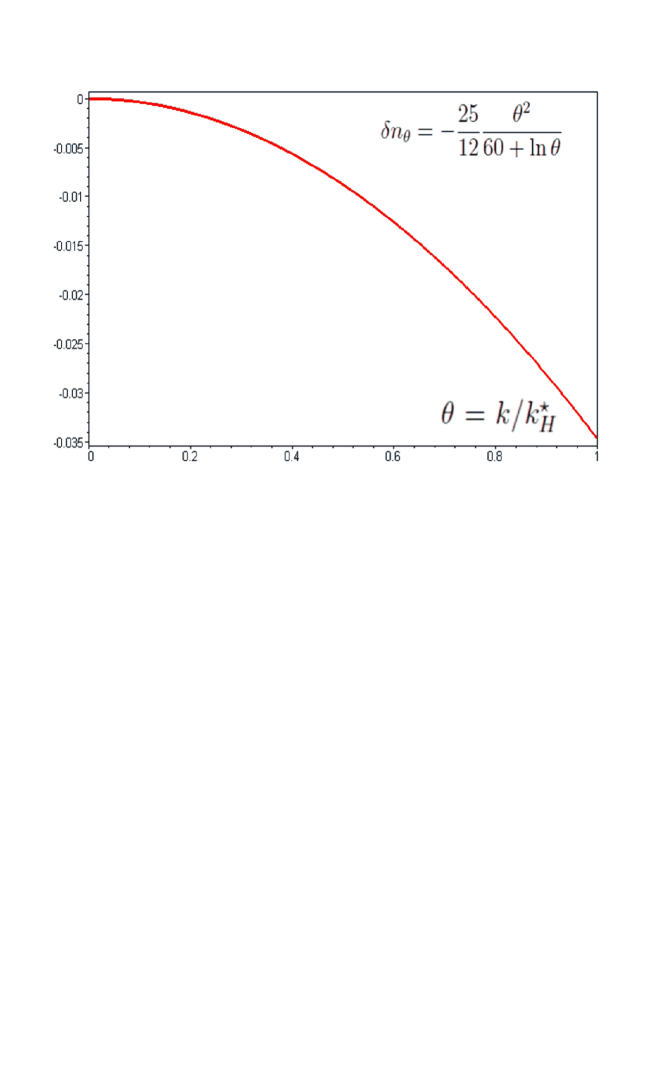
Figure 1: The figure shows $\delta n_{k}$ as a function of $\theta=k/k_{H}$. Notice that when the horizon entry (i.e., after inflation when $\theta=\theta_{*}=k_{*}/k_{H_{*}}=1$), the value of $\delta n_{k}$ is close to $\delta n_{k_{*}}\simeq-0.035$. In all our calculations we have taken into account the value $k_{H_{*}}=\sigma e^{60}$ as the wavenumber related to the horizon wavelength when, after inflation, the horizon entry.

The figure (1) shows $\delta n_{k}$ as a function of $\theta$. Notice that $\delta n_{k}$ decreases almost quadratically as the wavelength decreases. When the horizon entry (i.e., after inflation when $\theta=\theta_{*}=k_{*}/k_{H_{*}}=1$), the value of $\delta n_{k}$ is close to $\delta n_{k_{*}}\simeq-0.035$. However, during inflation the cosmological scales wavenumbers are $k/k_{H}<10^{-3}$ that corresponds with $\delta n_{k}>-10^{-6}$. Notice that we have taken into account the value $k_{H_{*}}=\sigma e^{60}$ as the wavenumber related to the horizon wavelength when, after inflation, the horizon entry.

5 Final Comments

We have shown how primordial electromagnetic fields and inflaton fluctuations can be generated jointly during inflation using a semiclassical approach to GEMI. We have used simultaneously the Lorentz and the Feynman gauges. The first one assures that the balance of each component of any external current to be null, and the second one is more restrictive, because assures that each direction (insider or outsider) of each component of the current to be zero. This is done with the aim to assure a 5D vacuum on the 5D Ricci flat metric (12). In correspondence with this concept of vacuum, we have defined a 5D totally kinetic Lagrangian density ${\cal L}_{f}=-\frac{1}{4}Q^{2}$, which is totally absent of any kind of interactions.

One of the important facts is that our formalism is naturally not conformal invariant on the effective 4D metric (23), which make possible the super adiabatic amplification of the modes of the electromagnetic fields during inflation in a comoving frame on cosmological (super Hubble) scales.

In this paper we have analyzed the simplest nontrivial configuration field: $\bar{A}^{b}=\left[0,0,0,0,\bar{\phi}(t,\psi_{0})\right]$. For this configuration of the background fields, the background inflaton field must be a constant on the metric (23) to satisfy the Einstein background equations in a de Sitter expansion: $\bar{\phi}(t,\psi_{0})=\bar{\phi}_{0}$. Then, in the model here developed, the expansion of the universe is driven by the background inflaton field $\bar{\phi}_{0}$ and background electromagnetic fields are excluded to preserve global isotropy. Notice that back reaction effects are not included, because the EM field does not contribute to the background expansion of the universe[18], but however comes into play an important role at the perturbative level as vectorial metric fluctuations which are the geometrical reaction to the vector physical fields[19].

To describe the effective 4D dynamics of the fields, we impose the effective 4D Lorentz gauge ${}^{(4)}\nabla_{\mu}A^{\mu}=0$, given simultaneously by conditions (24) and (25). Therefore, the origin of the generation of the seed of electromagnetic fields and the inflaton field fluctuations during inflation can be jointly studied. The dynamics of $\delta A^{\mu}$ on the effective 4D metric (23) obey a Proca equation with sources where the effective mass of the electromagnetic field fluctuations is induced by the foliation $\psi=\psi_{0}=1/H_{0}$. From the point of view of a relativistic observer this foliation imply that the component of the penta-velocity $U^{\psi}={d\psi\over dS}=0$.

We have obtained that for small values of $\nu$ a nearly scale-invariant long wavelengths power spectrum for $\left<B^{2}\right>^{1/2}$, which grows as $a$ during inflation on a comoving frame. However, on a physical frame it suffer a super adiabatical evolution, so that at the end of inflation is of the order of $10^{16}$ Gauss. After inflation we have supposed that the field evolves adiabatically as $a^{-2}$, to estimate the present day values on cosmological scales (for a physical frame): $\left.\langle B^{2}_{phys}\rangle^{1/2}\right|_{{\rm Now}}\simeq 10^{-52}$ Gauss[17]. On the other hand, the dominant terms in the amplitude of $\left<E^{2}\right>$ grows as $a^{2}$ on a comoving frame, and has a scale dependent power spectrum with a spectral index $n_{k}\simeq 3+\delta n_{k}$. This is the main result of this paper. This scale dependence is described by $\delta n_{k}$, which decreases quadratically as the scale decreases. In the limit case where $k\rightarrow 0$ (very large scales), one finds that $\delta n_{k=0}\rightarrow 0$. Finally, in what respect to the inflaton field fluctuations $\left<\delta\phi^{2}\right>$, we obtain that they are nearly scale invariant on cosmological scales, and the amplitude is freezed in agreement with the predictions of standard 4D inflation.

Appendix A The modes of the electric field

In order to solve the integrate in (77) we express all the Hankel functions in terms of the first kind Bessel functions $J_{\alpha}[x(t)]$, and $J_{-\alpha}[x(t)]$

$${\cal H}^{(1)}_{\alpha}(x)=\frac{J_{-\alpha(x)}-e^{-\alpha\pi i}J_{\alpha}(x)}{i\sin(\sigma\pi)},$$ (87)

$${\cal H}^{(2)}_{\alpha}(x)=\frac{J_{-\alpha(x)}-e^{\alpha\pi i}J_{\alpha}(x)}{-i\sin(\sigma\pi)},$$ (88)

and then we expand them in their series representation

$$J_{\alpha}[x(t)]=\sum_{m=0}^{\infty}\frac{(-1)^{m}}{m!\Gamma(1+m+\alpha)}\left(\frac{x(t)}{2}\right)^{2m+\alpha},$$ (89)

such that the product identity is[15]

$$(J_{\alpha}J_{\beta})[x(t)]=\sum_{m=0}^{\infty}\frac{(-1)^{m}}{m!}\frac{\Gamma(1+2m+\alpha+\beta)}{\Gamma(1+m+\alpha)\Gamma(1+m+\beta)\Gamma(1+m+\alpha+\beta)}\left(\frac{x(t)}{2}\right)^{2m+\alpha+\beta}.$$ (90)

The terms included in expression (77) are of the form,

$$J_{\gamma}(x(t))\int dte^{H_{0}t}(J_{\alpha}J_{\beta})[x(t)]=\frac{k}{2H_{0}}\sum_{m,n}^{\infty}\frac{(-1)^{m+n}}{m!n!}{\cal C}^{mn}_{\alpha,\beta,\gamma}\left(\frac{x(t)}{2}\right)^{2(m+n)-1+\alpha+\beta+\gamma},$$ (91)

$$J_{\gamma}(x(t))\int dt(J_{\alpha}J_{\beta})[x(t)]=\frac{1}{H_{0}}\sum_{m,n}^{\infty}\frac{(-1)^{m+n}}{m!n!}{\cal D}^{mn}_{\alpha,\beta,\gamma}\left(\frac{x(t)}{2}\right)^{2(m+n)+\alpha+\beta+\gamma},$$ (92)

where the coefficients ${\cal C}_{\alpha,\beta,\gamma}^{mn}$ and ${\cal D}_{\alpha,\beta,\gamma}^{mn}$ are defined by the following relations of the Gamma functions

$${\cal C}_{\alpha,\beta,\gamma}^{mn} = \frac{\Gamma(1+2m+\alpha+\beta)}{(1-2m-\alpha-\beta)\Gamma(1+m+\alpha+\beta)\Gamma(1+m+\alpha)\Gamma(1+m+\beta)\Gamma(1+n+\gamma)},$$ (93)

$${\cal D}_{\alpha,\beta,\gamma}^{mn} = \frac{\Gamma(1+2m+\alpha+\beta)}{(-2m-\alpha-\beta)\Gamma(1+m+\alpha+\beta)\Gamma(1+m+\alpha)\Gamma(1+m+\beta)\Gamma(1+n+\gamma)}.$$ (94)

After some algebra, one arrives to the inhomogeneous solution for the modes of the electromagnetic field $A^{0}$

$$X^{(0)}(t,k,\psi_{0})=\frac{i}{\sin(\sigma\pi)}\sqrt{\frac{\pi^{3}}{H_{0}}}\left(\frac{2}{k}\right)^{\frac{3}{2}}\sum_{m,n}^{\infty}\frac{(-1)^{m+n}}{m!n!}\left(\frac{x(t)}{2}\right)^{2(m+n)}\sum_{s=1}^{3}{\cal E}^{mn}_{p_{s}}\left(\frac{x(t)}{2}\right)^{p_{s}},$$ (95)

where $x(t)=k\,e^{-H_{0}t}$. The sum over $s$ goes through three different powers. The coefficients ${\cal E}^{mn}_{p_{s}}$ depend on the parameters $\mu,\sigma$ and sum on indices $m,n$ in the following way

$$p_{1}={3\over 2}+\mu,\,\,{\cal E}^{mn}_{p_{1}}=\frac{e^{\mu\pi i}}{\sin(\mu\pi)}\left[\frac{({3\over 2}-\mu)}{2}\left(-{\cal C}_{\mu,\sigma,-\sigma}^{mn}+{\cal C}_{\mu,-\sigma,\sigma}^{mn}\right)-{\cal D}_{\mu-1,-\sigma,\sigma}^{mn}+{\cal D}_{\mu-1,\sigma,-\sigma}^{mn}\right],$$ (96)

$$p_{2}={3\over 2}-\mu,\,\,{\cal E}^{mn}_{p_{2}}=\frac{1}{\sin(\mu\pi)}\frac{({3\over 2}-\mu)}{2}\left({\cal C}_{-\mu,\sigma,-\sigma}^{mn}-{\cal C}_{-\mu,-\sigma,\sigma}^{mn}\right),$$ (97)

$$p_{3}={7\over 2}-\mu,\,\,{\cal E}^{mn}_{p_{3}}=-\frac{1}{\sin(\mu\pi)}({\cal D}_{1-\mu,\sigma,-\sigma}^{mn}-{\cal D}_{1-\mu,-\sigma,\sigma}^{mn}).$$ (98)

The inhomogeneous solution, $X^{j}(k,t,\psi_{0})$, of $A^{j}$, has essentially three contribution terms. For simplicity, lets split the sources in the following way:

$${\cal F}_{1}^{j}=2H_{0}^{2}(i\,k^{j})\,W^{(0)}(k,t,\psi_{0}),\ \ \ \ {\cal F}_{2}^{j}=2(i\,k^{j})\,H_{0}^{3}\phi(k,t,\psi_{0}),\ \ \ \ {\cal F}_{3}^{j}=2H_{0}^{2}(i\,k^{j})\,X^{(0)}(k,t,\psi_{0}).$$ (99)

Hence, the final solution of (77), written as $X^{j}=X^{j}_{1}+X^{j}_{2}+X^{j}_{3}$, after using $k^{j}=k\,e^{j}$ ($e^{j}$ being an unitary vector), is given by the expressions

$$X_{1}^{j}(k,t,\psi_{0}) = -\frac{e^{j}}{\sin^{2}(\sigma\pi)}\sqrt{\frac{\pi^{3}}{H_{0}}}\left(\frac{2}{k}\right)^{\frac{3}{2}}\sum_{n}^{\infty}\frac{(-1)^{n}}{n!}$$ (100)

$$\times \left\{\frac{H_{0}t}{\Gamma(1-\sigma)\Gamma(1+\sigma)}\left[\frac{(x/2)^{\frac{5}{2}-\sigma}}{\Gamma(1+n-\sigma)}+\frac{(x/2)^{\frac{5}{2}+\sigma}}{\Gamma(1+n+\sigma)}\right]\right.$$

$$+ \sum_{m=1}^{\infty}\frac{(-1)^{m}}{m!}\left[{\cal D}_{-\sigma,\sigma,-\sigma}^{mn}\left(\frac{x}{2}\right)^{\frac{5}{2}-\sigma+2m}+e^{\sigma\pi i}{\cal D}_{\sigma,-\sigma,\sigma}^{mn}\left(\frac{x}{2}\right)^{\frac{5}{2}+\sigma+2m}\right]$$

$$- \left.\sum_{m=0}^{\infty}\frac{(-1)^{m}}{m!}\left[e^{\sigma\pi i}{\cal D}_{\sigma,\sigma,-\sigma}^{mn}\left(\frac{x}{2}\right)^{\frac{5}{2}+\sigma+2m}+{\cal D}_{-\sigma,-\sigma,\sigma}^{mn}\left(\frac{x}{2}\right)^{\frac{5}{2}-\sigma+2m}\right]\right\}\,\left(\frac{x}{2}\right)^{2n},$$

$$X_{2}^{j}(k,t,\psi_{0}) = -\frac{e^{j}}{\sin(\sigma\pi)}\sqrt{\frac{\pi^{3}}{H_{0}}}\left(\frac{2}{k}\right)^{\frac{1}{2}}\sum_{m,n}^{\infty}\frac{(-1)^{m+n}}{m!n!}\left(\frac{x(t)}{2}\right)^{2(m+n)}\sum_{s=1}^{2}2{\cal E}^{mn}_{r_{s}}\left(\frac{x(t)}{2}\right)^{r_{s}},$$ (101)

with

$$r_{1} = 3/2+\mu,\ \ \ \ \ \ \ \ \ \ {\cal E}^{mn}_{r_{1}}=-\frac{e^{\mu\pi i}}{\sin(\mu\pi)}\left({\cal C}_{\mu,\sigma,-\sigma}^{mn}-{\cal C}_{\mu,-\sigma,\sigma}\right),$$ (102)

$$r_{2} = 3/2-\mu,\ \ \ \ \ \ \ \ \ \ {\cal E}^{mn}_{r_{2}}=\frac{1}{\sin(\mu\pi)}\left({\cal C}_{-\mu,\sigma,-\sigma}^{mn}-{\cal C}^{mn}_{-\mu,-\sigma,\sigma}\right).$$ (103)

Finally, the contribution of the inhomogeneous source is

$$X_{3}^{j}(k,t,\psi_{0})= -\frac{e^{j}}{\sin(\sigma\pi)}\sqrt{\frac{\pi^{3}}{H_{0}}}\left(\frac{2}{k}\right)^{\frac{1}{2}}\frac{4\pi}{\sin(\sigma\pi)}$$ (104)

$$\times\sum_{l,m,n,h}^{\infty}\frac{(-1)^{l+m+n+h}}{l!\,m!\,n!\,h!\,\Gamma(1+l+\sigma)\Gamma(1+h-\sigma)}\left(\frac{x(t)}{2}\right)^{2(l+m+n+h)}$$

$$\times\sum_{s=1}^{3}{\cal E}^{mn}_{p_{s}}\frac{\sigma\,}{\left[p_{s}+2(l+m+n)-\frac{5}{2}\right]^{2}-\sigma^{2}}\left(\frac{x(t)}{2}\right)^{p_{s}}.$$

Appendix B Calculation of the spectrum for the electric field fluctuations

It is important to notice that $\dot{X}^{j}_{1}$ has appreciable differences with the other terms in (79); the one has a preceding factor $k^{-3/2}$, while the others ($iK^{j}X^{0}$, $\dot{X}^{j}_{2}$ and $\dot{X}^{j}_{3}$) are proportional to $k^{-1/2}$. Furthermore, $\dot{X}^{j}_{1}$ has terms with the linear factor $H_{0}t$ while the others doesn’t.

Taking into account the last observation we arrange the power spectrum as follows

$${\cal P}_{k}(t)=k^{2}\sum_{q=0}^{\infty}a_{q}(ke^{-H_{0}t})^{\beta_{0}+q}+k\sum_{q=0}^{\infty}b_{q}(t)(ke^{-H_{0}t})^{\gamma_{0}+q}+\sum_{q=0}^{\infty}c_{q}(t)(ke^{-H_{0}t})^{\rho_{0}+q}.$$ (105)

The coefficients $a_{q}$ are all calculable from quadratics and cross products of: $iK^{j}X^{0}$, $\dot{X}^{j}_{2}$ and $\dot{X}^{j}_{3}$. The coefficients $b_{q}(t)=b^{(1)}_{q}+b_{q}^{(2)}t$ are linear in time and come from products of $\dot{X}^{j}_{1}$ with the others. Finally, the coefficients $c_{q}(t)=c^{(1)}_{q}+c^{(2)}_{q}t+c^{(3)}_{q}t^{2}$ are quadratic in time and are found from $\sum_{j}|\dot{X}^{j}_{1}|^{2}$. The lowest powers from which each term in the series begin are: $\beta_{0}=3-2\mu$, $\gamma_{0}=-2+\mu+\sigma$ and $\rho_{0}=-4+2\sigma$.

Since the terms that grow stronger are those that involve $a_{q}$, we shall restrict our study just to these. We shall try to obtain the power spectrum in a power-law form

$${\cal P}_{k}(t)=C(t)k^{n_{k}-1}.$$ (106)

This will automatically lead us to a scale dependent spectral index $n_{k}$, that it is found to be

$$n_{k}=3-\beta_{0}+\frac{\ln\left[1+\sum_{i=1}^{\infty}\frac{a_{i}}{a_{0}}(ke^{-H_{0}t})^{\beta_{0}+i}\right]}{\ln(k)},$$ (107)

where $C(t)=a_{0}e^{-\beta_{0}H_{0}t}$ depends on the first coefficient and the first power. We may write

$$n_{k} = n_{0}+\delta n_{k},$$ (108)

$$n_{0} = 3-\beta_{0}=2\mu\simeq 3,$$ (109)

$$\delta n_{k} = \frac{\ln\left[1+\sum_{i=1}^{\infty}\frac{a_{i}}{a_{0}}(ke^{-H_{0}t})^{\beta_{0}+i}\right]}{\ln(k)}.$$ (110)

Since the values of $k$ are related to super Hubble wavelengths : $0<k<\theta\sigma e^{H_{0}t}$ (and assuming that $\theta\sigma\ll 1$), we see that $0<ke^{-H_{0}t}\ll 1$ and therefore it is pertinent a perturbative analysis in powers of $\theta\sigma$. In this case the dominant spectral index comes from $n_{0}=2\mu$, and $\delta n_{k}$ are perturbative corrections. The integration of any of the power spectrums (105) or (106) provide us the amplitude for electric fields

$$\int_{0}^{\theta k_{H}}\frac{dk}{k}{\cal P}_{k}(t)\simeq e^{2H_{0}t}\left[\frac{a_{0}(\theta\sigma)^{2+\beta_{0}}}{2+\beta_{0}}+\frac{a_{1}(\theta\sigma)^{3+\beta_{0}}}{3+\beta_{0}}+\frac{a_{2}(\theta\sigma)^{4+\beta_{0}}}{4+\beta_{0}}+...\right].$$ (111)

If we only stay with $n_{0}$, this would mean we are cutting the previous expression just to the first term and only the coefficient $a_{0}$ will appear. But if we keep to first order corrections in $\delta n_{k}$, we can see that the factor $a_{1}/a_{0}$ appears in the correction. In general we shall obtain that to $N$th-order correction, the first $N$ coefficients will appear to each order respectively.

In what follows we shall fix the spectral indices of the inflaton as $\mu=3/2+\epsilon$, where $\epsilon=-m^{2}/2$ and $m^{2}$ is associated to the measured spectral scalar index $n_{s}\simeq 0.96$ [16]: $m^{2}\simeq-0.04$. The spectral index of the vector fields is fixed so as to give a nearly scale invariant spectrum of the magnetic fields $\sigma=5/2+\eta$, with $\eta=-\nu^{2}/5$. For a similar spectrum to whole of the inflaton field it is expected to $\nu^{2}$ to be negative, but $|\nu^{2}|\ll 1$.

Studying just the terms that grow faster, as $e^{2H_{0}t}$, and considering sufficiently large scales $\theta\ll 1$, we shall cut the power series to the first two terms. For the previous values of $\mu$ and $\sigma$ there is no $a_{1}$, since the power series begins after the $a_{0}$ term, in $a_{2}$.

Since $(3/2-\mu){\cal E}^{mn}_{r_{2}}=2{\cal E}^{mn}_{p_{2}}$, to obtain $a_{0}$ only we need to find ${\cal E}^{00}_{p_{2}}$ in (97)

$${\cal E}^{00}_{p_{2}}=\frac{\epsilon}{10\pi^{3/2}}\left[\frac{1}{\epsilon-\eta}-\frac{1}{5}\right],$$ (112)

and then

$$a_{0}=\frac{H_{0}^{4}}{2\pi^{2}25}\epsilon^{2}\left[\frac{1}{\epsilon-\eta}-\frac{1}{5}\right]^{2}\left[1+\frac{2/5}{\epsilon-\eta}\right]^{2}.$$ (113)

Since both, $\epsilon$ and $\eta$ are respectively small departures from $\mu$ and $\sigma$, then we obtain that $(\epsilon-\eta)^{-1}\gg 1$. We notice that $2/5(\epsilon-\eta)^{-1}$ comes from the solution $X^{j}_{3}$, that considers only the contribution from the inhomogeneous solution of $X^{0}$, coupled to the effective inflaton. This means that here the most relevant solution is $X^{j}_{3}$, and only considering this solution one obtains

$$a_{0}=\frac{2H_{0}^{4}}{\pi^{2}5^{4}}\frac{\epsilon^{2}}{(\epsilon-\eta)^{4}},$$ (114)

with a spectral index $n_{0}=3$ and $\delta n_{k}=0$.

References

-
[1]
H. Toshiro, N. Sugiyama and R. Banerjee, Phys. Rev.
D73: 023002 (2006);
D. G. Yamazaki, K. Ichiki, T. Kajino and G. J. Mathews, Phys. Rev. D77: 043005 (2008);
F. Finelli, F. Paci and D. Paoletti, Phys. Rev. D78: 023510 (2008). - [2] M. S. Turner and L. M. Widrow, Phys. Rev. D37: 2743 (1988).
- [3] D. Grasso and H. R. Rubinstein, Phys. Rept. 348: 163 (2001).
- [4] M. Giovannini, Int J. Mod. Phys. D13: 391 (2004).
- [5] M. Giovannini, Class. Quant. Grav. 23: R1 (2006).
-
[6]
J. E. Campbell, A course of Differential
Geometry (Charendon, Oxford, 1926);
L. Magaard, Zur einbettung riemannscher Raume in Einstein-Raume und konformeuclidische Raume. (PhD Thesis, Kiel, 1963);
S. Rippl, C. Romero, R. Tavakol, Class. Quant. Grav. 12: 2411 (1995);
F. Dahia, C. Romero, J. Math. Phys.43: 5804 (2002);
F. Dahia, C. Romero, Class. Quant. Grav. 22: 5005 (2005). -
[7]
A. Raya, J. E. Madriz Aguilar, M. Bellini, Phys.
Lett. B638: 314 (2006);
J. E. Madriz Aguilar, M. Bellini, Phys. Lett. B642: 302 (2006);
F. A. Membiela, M. Bellini, Nuovo Cim. B123: 241 (2008);
F. A. Membiela, M. Bellini, Phys. Lett. B674: 152 (2009). -
[8]
B. Ratra, Astrophys. J. 391: L1 (1992);
A. D. Dolgov, Phys. Rev. 48: 2499 (1993);
F. D. Mazzitelli and F. M. Spedalieri, Phys. Rev. bf D52: 6694 (1995);
M. Gasperini, M. Giovannini and G. Veneziano, Phys. Rev. Lett. 75: 3796 (1995);
E. A. Calzetta, A. Kandus and F. D. Mazzitelli, Phys. Rev. D57: 7139 (1998);
M. S. Turner and L. M. Widrow, Phys. Rev. D37: 2743 (1998);
O. Bertolami and D. F. Mota, Phys. Lett. B455: 96 (1999);
A. -C. Davis, K. Dimopoulos, T. Prokopec and O. Törnkvist, Phys. Lett. B501: 165 (2001);
B. A. Bassett, G. Pollifrone, S. Tsujikawa and F. Viniegra, Phys. Rev. D63: 103515 (2001);
M. Gasperini, Phys. Rev. D63: 047301 (2001);
G. Lambiase and A. R. Prasanna, Phys. Rev. D70: 063502 (2004);
M. Giovannini, Phys. Rev. D76: 103508 (2007);
K. Bamba, S. Nojiri, S. D. Odintsov, Phys. Rev. D77: 123532 (2008);
K. Bamba, N. Ohta, S. Tsujikawa, Phys. Rev. D78: 043524 (2008);
K. Bamba, C. Q. Geng, S. H. Ho, JCAP 0811: 013 (2008). - [9] N. D. Birrell and P. C. W. Davies, Quantum fields in curved space. Cambridge University Press, Cambridge (1982).
- [10] D. S. Ledesma and M. Bellini, Phys. Lett. B581: 1 (2004).
- [11] J. Ponce de Leon, Gen. Rel. Grav. 20: 539 (1988).
- [12] M. Bellini, H. Casini, R. Montemayor, P. Sisterna, Phys. Rev. D: 7172 (1996).
- [13] F. A. Membiela and M. Bellini, Phys. Lett. B685: 1 (2010); Erratum-ibid. 688: 356 (2010).
- [14] T. Kahniashvili, L. Kisslinger and T. Stevens, Phys. Rev. D81: 023004 (2010).
- [15] See eq. in M. Abramowithz and A. Stegun, Handbook of Mathematical functions: Dover publications. NY (1972).
- [16] Review of Particle Physics. Phys. Lett. B667: 103-105 (2008).
-
[17]
C. L. Bennett et al, Astrophys. J. Suppl. 148: 1 (2003);
C. A. Clarkson, A. A. Coley, R. Maartens and C. G. Tsagas, Class. Quant. Grav. 20, 1519 (2003);
M. Giovannini, Phys. Rev. D79: 121302 (2009). - [18] R. Durrer, The Cosmic Microwave Background (Cambridge University Press, Cambridge, UK, 2008).
- [19] Ruth Durrer, Lukas Hollenstein, Rajeev Kumar Jain. Can slow roll inflation induce relevant helical magnetic fields?. E-print: arXiv:1005.5322.