Vibrational wave packet induced oscillations in two-dimensional electronic spectra.
I. Experiments

Abstract

This is the first in a series of two papers investigating the effect of electron-phonon coupling in two-dimensional Fourier transformed electronic spectroscopy. We present a series of one- and two-dimensional nonlinear spectroscopic techniques for studying a dye molecule in solution. Ultrafast laser pulse excitation of an electronic transition coupled to vibrational modes induces a propagating vibrational wave packet that manifests itself in oscillating signal intensities and line-shapes. For the two-dimensional electronic spectra we can attribute the observed modulations to periodic enhancement and decrement of the relative amplitudes of rephasing and non-rephasing contributions to the total response. Different metrics of the two-dimensional signals are shown to relate to the frequency-frequency correlation function which provides the connection between experimentally accessible observations and the underlying microscopic molecular dynamics. A detailed theory of the time-dependent two-dimensional spectral line-shapes is presented in the accompanying paper [T. Mančal et al., arXiv:1003.xxxx].

^∗ alexandra.nemeth@univie.ac.at

I Introduction

Coherent wave packet generation in the manifolds of molecular exited states takes place if the excitation pulses are spectrally broad enough to coherently excite a number of vibrational or electronic levels. Femtosecond (fs) laser pulses meet this criterion in a number of molecular systems and experiments employing such pulses often show signatures of wave packet motion. Modulations of signal intensities induced by vibrational wave packet motion have been observed in a number of nonlinear spectroscopic experiments, including pump-probe (PP) Zewail (1993); Fragnito et al. (1989); Kobayashi et al. (2001), transient grating (TG) Larsen et al. (2001), and a variety of photon-echo spectroscopies Becker et al. (1989); Schoenlein et al. (1993); Larsen et al. (2001); de Boeij et al. (1998); de Boeij et al. (1996a). A number of theoretical investigations supported the conclusions drawn in these experiments Yan and Mukamel (1990); Pollard et al. (1990, 1992); Dhar et al. (1994); Ohta et al. (2001). The influence of intramolecular vibrations should be expected consequently also in the recently implemented heterodyne-detected two-dimensional electronic spectroscopy (2D-ES) technique Hybl et al. (1998); Tian et al. (2003); Cowan et al. (2004); Brixner et al. (2004); Borca et al. (2005); Gundogdu et al. (2007); Nemeth et al. (2008); Milota et al. (2009), which is based on the correlation of electronic coherences evolving during two time periods. 2D electronic spectra recorded for distinct waiting times provide information on coupling patterns and evolution of populations and coherences via line-shape modulations and the appearance and disappearance of cross peaks Hybl et al. (2002); Tian et al. (2003); Borca et al. (2005); Brixner et al. (2005); Stiopkin et al. (2006); Nemeth et al. (2008, 2009).

Recent theoretical works on model dimer Pisliakov et al. (2006); Cheng and Fleming (2008) and trimer Cheng et al. (2007) systems, and experimental investigations on excitonic complexes Engel et al. (2007); Milota et al. (2009) and conjugated polymers Collini and Scholes (2009) reported on signatures of electronic wave packets in 2D electronic spectra resulting from coherent excitation of several electronic levels. Possible enhancement of the energy transfer efficiency in photosynthetic light harvesting complexes, due to the presence of excitonic wave packets, was suggested by Engel et al. Engel et al. (2007). An assignment of the observed spectral modulations to an excitonic wave packet motion was made, based on a good agreement of the experiment with the predictions of an excitonic model Pisliakov et al. (2006); Engel et al. (2007). In the general case, however, contributions of vibrational wave packet motion cannot be excluded and it is therefore of high importance to study the vibrational case separately. To the best of our knowledge, vibrational effects in 2D-ES have been addressed so far only theoretically Gallagher-Faeder and Jonas (1999); Egorova et al. (2007) and in our recent work on the same molecular system Nemeth et al. (2008).

To study the effect of vibrational coherence without perturbations from additional electronic levels, a two-level system is preferential. Quantum-chemistry calculations (cf. Section II) indicate that N,N’-bis(2,6-dimethylphenyl)perylene-3,4,9,10-tetracarboxylicdiimide (PERY), when excited at 20000 cm^-1, can be approximated as a two-level electronic system with a number of vibrational modes coupled to the electronic transition Larsen et al. (1999). In the linear absorption spectrum of PERY in solution four well resolved vibrational peaks with a frequency separation of $\approx$1400 cm^-1 can be discerned (Fig. 1a). In contrast to a recent work by Tekavec et al. Tekavec et al. (2009), in which white light pulses where used to probe the vibronic dynamics, this progression can not be covered with the bandwidth of our laser pulses (900 cm^-1). However, by tuning the central excitation energy approximately to the center of the lowest energy peak, nonlinear spectroscopic signals such as transient grating (TG) and three-pulse photon echo peak shift (3PEPS) have been shown to be modulated by a low frequency (140 cm^-1) vibrational mode Larsen et al. (1999).

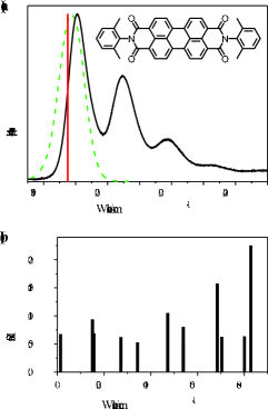
Figure 1: (a) Linear absorption spectrum of PERY in toluene (black solid line) and spectrum of the excitation pulses (green dashed line). The red line indicates the position of the lowest energy transition obtained from ZINDO/S calculations. The inset shows the chemical structure of PERY. (b) Huang-Rhys factors determined from semiemprical AM1 calculations. Only modes that posses Huang-Rhys factors larger than 0.005 are plotted.

In this contribution we investigate experimentally how coherent excitation of several vibrational levels influences 2D electronic correlation and relaxation spectra. To this end 2D electronic spectra of PERY have been recorded for 20 waiting times $t_{2}$ ranging from 0 to 800 fs covering several periods of pronounced vibrational modulations of the spectra. In a recent work on the same molecular system we have shown that this low frequency mode induces a periodic change in the ellipticity of the real (absorptive) part and in the slope of the nodal line separating the positive and negative contribution of the imaginary (dispersive) part Nemeth et al. (2008). Building up on these qualitative observations, in this contribution we will assign these modulations to periodic enhancement and decrement of the rephasing and non-rephasing signal parts and establish connections to the frequency-frequency correlation function M(t). In the accompanying paper Ref. Mančal et al. (2009) (paper II) the underlying theory is presented.

This paper is organized as follows. We start in Section II with a quantum- chemical characterization of the molecule under investigation. The experimental details are provided in Section III. In Section IV two-dimensional electronic spectra are presented and connections to the frequency-frequency correlation function are established. We close in Section V with some concluding remarks. The appendix contains a comparison to related one-dimensional four-wave mixing signals.

II Quantum-chemical calculations

This section characterizes PERY theoretically and spectroscopically with respect to its two-dimensional $\pi$-conjugation by means of quantum-chemical calculations. The electronic ground state geometry of PERY has been optimized using Density Functional Theory (DFT) Parr and Yang (1991) based on the Becke’s three parameter hybrid functional using the Lee, Yang and Parr correlation functional (B3LYP) Becke (1996). The polarized split-valence SV(P) basis set Dunning and Hay (1977) has been used. The obtained optimal structures were checked by normal mode analysis (no imaginary frequencies for all optimal geometries). Based on the optimized geometry, the vertical transition energies and oscillator strengths between the initial and final states have been calculated using the Configuration Interaction Singles (CIS) method Foresman et al. (1992) based on the semiempirical ZINDO/S (Zerner’s Intermediate Neglect of Differential Overlap) Hamiltonian Zerner et al. (1980). For the ZINDO/S calculations, the single excitations from the 10 highest occupied to the 10 lowest unoccupied molecular orbitals were considered. The DFT calculations were done using the Turbomole 5.7 package Ahlrichs et al. (1989) and the optical transitions were computed using the Argus Lab software Thompson (2004). The evaluated theoretical values are used for the interpretation of experimental spectroscopic measurements.

The optimal geometry of D₂ symmetry exhibits a planar central part (Fig. 2a). The orientation of the lateral aromatic rings and the core skeleton is nearly perpendicular (dihedral angles of 81.2^∘) causing a negligible $\pi$-conjugation between these molecular fragments. The lateral rings are sterically hindered due to the presence of methyl groups in ortho-position. The opposite mutual arrangement of the neighboring lateral rings is not parallel as can be perceived from the right part of Fig. 2a.

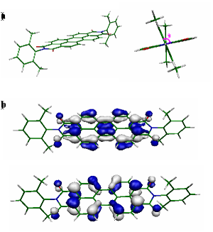
Figure 2: (a) Side and front views on the B3LYP/SV(P) optimal structure of PERY in the electronic ground state. (b) Visualization of the HOMO (bottom) and LUMO (top) obtained from ZINDO/S//B3LYP/SV(P) calculations.

The photophysical properties of PERY are primarily determined by the planar geometry of the central part and the related size of the $\pi$-conjugation. The experimental absorption spectrum of PERY in toluene (Fig. 1a) can be characterized by an intense absorption band with four peaks which are detected in the spectral range of 18000 to 24000 cm^-1. The equidistant energy difference (1400 cm^-1) between the four peaks indicates a harmonic character of the vibrational progression. The calculated vertical ZINDO/S excitation energies and the oscillator strengths are in good agreement with the experimental absorption spectrum. The ZINDO/S method was parametrized for spectroscopic properties of the $\pi$-conjugated aromatic systems and gives transition energies of 18725 cm^-1 with an oscillator strength f$=1.7814$, 28631 cm^-1 (f$=0.0001$), 31929 cm^-1 (f$=0.0002$), and 34536 cm^-1 (f$=0.8228$). The lowest energy transition is depicted as red line in Fig. 1a. The absence of other intensive electronic transitions in the region between 18000 and 24000 cm^-1 indicates the vibronic origin of the progression observed in the experimental absorption spectrum. Therefore, the first and most intensive peak in the experimental record can be attributed to the $0\rightarrow 0$ vibronic transition. In this context it is useful to examine the ZINDO/S HOMO and LUMO of the molecule. The HOMO-LUMO excitation plays a dominant role in this energetically lowest optical transition according to the frontier molecular orbital theory, with its contribution being more than 30%. These selected ZINDO/S orbitals are visualized in Fig. 2b, demonstrating that both orbitals are delocalized over the center of the core part only. The lobes of the LUMO are oriented more or less perpendicular to the lobes of the HOMO. The shape of the LUMO compared to those of the HOMO indicates that the optical excitation is spread from the central atoms of the core towards the nitrogen atoms.

In order to determine the origin of the vibronic motion reflected in the linear and nonlinear spectroscopic experiments, vibrational line spectra have been calculated. The complete set of computed vibrational frequencies and intensities together with a visualisation of the most dominant modes and Huang-Rhys factors are collected in the Supporting Information. For determining the Huang-Rhys factors semiemprical AM1 calculations were performed using the Mopac program package 2002 Stewart (Fujitsu Ltd. 2001). The calculated vibrational spectrum possesses 210 fundamentals between 13 and 3243 cm^-1. With the limited bandwidth of our excitation pulses we can only cover modes up to frequencies of approximately 900 cm^-1. From Fig. 1b, in which modes with a Huang-Rhys factor larger than 0.005 are plotted, it becomes obvious that only a few modes contribute significantly to the observed spectroscopic response.

III Experimental

PERY was purchased from Sigma-Aldrich and used without further purification. Solutions with a concentration of $3\cdot 10^{-4}$ M were prepared by dissolving PERY in toluene (spectrophotometric grade, Merck), sonication for $\approx$10 minutes, and filtration to remove undissolved residues.

Pulse generation is accomplished by a regenerative titanium-sapphire amplifier system (RegA 9050, Coherent Inc.) operating at a repetition rate of 200 kHz. Conversion into the visible spectral region is attained with a noncollinear optical parametric amplifier (NOPA) Piel et al. (2006). For our present study the central excitation energy was set to 18800 cm^-1 (FWHM 920 cm^-1) and the pulses were attenuated to 10 nJ per pulse at the sample position. Second-order dispersion is eliminated with a sequence of fused-silica prisms, while chirped mirrors compensate for third-order dispersion, yielding a pulse duration of 16 fs. The pulse duration is determined with an improved version of spectral phase interferometry for direct electric field reconstruction (SPIDER), zero additional phase (ZAP) SPIDER Baum and Riedle (2005), and cross-checked with SHG-FROG Trebino et al. (1997).

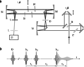
Figure 3: (a) Schematic setup for recording 2D electronic spectra. BS $\ldots$ beamsplitter, CP $\ldots$ compensation plate, SM $\ldots$ spherical mirror, DOE $\ldots$ diffractive optical element, WP $\ldots$ wedge pair, ND $\ldots$ neutral density filter, S $\ldots$ sample, L $\ldots$ lens, CCD $\ldots$ charge coupled device camera. (b) Designation of pulses and time delays in four wave mixing experiments.

Our approach for recording 2D electronic spectra is based on a diffractive-optics based setup following the experimental configuration reported in Ref. Cowan et al. (2004); Brixner et al. (2005); Moran et al. (2006) (Fig. 3a). A 50/50 beam splitter (BS) splits the NOPA output into two beams of equal intensity, one of which can be delayed with respect to the other by a computer controlled delay stage to introduce delay $t_{2}$ (cf. Fig. 3b for a definition of time delays). A diffractive optical element (DOE), optimized for diffraction into $\pm$first order, is used to split the two beams focused onto it into four beams Cowan et al. (2004). From this point on, all four beams are reflected from common mirrors to maintain the phase correlations Cowan et al. (2004); Brixner et al. (2004). A spherical mirror (SM) after the transmission grating parallelizes the four beams which are arranged to form the four corners of a square. Pulse $\mathbf{k_{2}}$ passes through a pair of glass wedges (WP) that are oriented in an anti-parallel fashion Brixner et al. (2004). By moving one of the wedges with a computer controlled delay stage, the amount of glass in the beam path and therefore the delay of the pulse is changed without introducing lateral beam shifts. This configuration allows for precise delay movements (5.3 as) without influencing the phase stability of the phase locked pulse pair and is used to introduce delay $t_{1}$. Pulses $\mathbf{k_{1}}$ and $\mathbf{k_{3}}$ pass through equivalent but static wedge pairs to balance the dispersion. The LO is attenuated by a neutral density filter (ND) by four to five orders of magnitude and reaches the sample approximately 550 fs before the other pulses. All four beams are focused by a spherical mirror onto the sample to generate the nonlinear signal. In order to avoid unwanted signals from a cuvette window and to prevent precipitation of the sample on the cell windows, a wire-guided gravity driven jet Tauber et al. (2003); Laimgruber et al. (2006) is implemented, yielding a film of approximately 200 $\mu$m thickness. Due to the square geometry of the excitation beams and the LO, the signal propagation direction is coincident with the propagation direction of the LO allowing for heterodyne detection of the signal field with the LO. Data acquisition is accomplished by means of a thermoelectrical cooled charge-coupled-device (CCD) spectrometer. A 2400 lines/mm grating in combination with a 1024 pixel array allows for a spectral resolution of 3.3 cm^-1 in $\omega_{3}$.

For recording 2D electronic spectra, $t_{2}$ is fixed at a certain value and $t_{1}$ is scanned over $\pm$100 fs with a step size of 0.65 fs to fulfill the Nyquist sampling criterion. The electric field of the signal as a function of frequency ($\omega_{3}$) is reconstructed by Fourier transform of each interferogram (for every $t_{1}$-step), filtering and back Fourier transform Lepetit and Joffre (1996). Fourier transform along $t_{1}$ yields the second frequency dimension $\omega_{1}$. The frequency resolution in $\omega_{1}$ is solely determined by the maximal temporal separation between pulses $\mathbf{k_{1}}$ and $\mathbf{k_{2}}$ and amounts to 26 cm^-1 in our experiments. In a final step the absolute phase of the 2D spectrum has to be determined. Since the PP signal does not depend on constant phase shifts of either the pump or the probe beam, it can be used for this purpose Jonas (2003). To this end the projection slice theorem is applied, that states that the projection of the real part of the 2D spectrum onto $\omega_{3}$ equals the spectrally resolved (SR) PP signal. By multiplying this projection by a factor of e^-iϕ and adjusting $\phi$ so that the projection matches the SRPP signal, the absolute phase of the 2D spectrum is recovered.

IV Results and Discussion

IV.1 Two-dimensional electronic spectra

With second-order nonlinear signals being symmetry-forbidden in isotropic media such as bulk liquids, the third-order nonlinearity is the lowest nonlinear order at which system-bath interactions and solute dynamics in liquids can be probed. The third-order nonlinear polarization $P^{(3)}(t_{1},t_{2},t_{3})$ is thereby induced by three interactions with pulsed electromagnetic fields (with wavevectors $\mathbf{k_{1}}$, $\mathbf{k_{2}}$, $\mathbf{k_{3}}$ and temporal separation $t_{1}$ and $t_{2}$) and it radiates the signal in the phase-matched directions $\mathbf{\pm k_{1}\pm k_{2}\pm k_{3}}$. Depending on the scanning procedure, the detection direction (phase matching), and the detection scheme (time vs. frequency resolved; homodyne vs. heterodyne detection), different techniques can be distinguished. In this subsection we focus on two-dimensional electronic spectroscopy, related one-dimensional four-wave mixing techniques are discussed in the Appendix.

In contrast to one-dimensional FWM techniques, where time- or frequency-integrating detection schemes project the full information content onto a single axis (i.e. intensity vs. time or frequency), 2D spectra provide a more complete picture by extending the dimensionality of representation. Selective excitation, competing with high temporal resolution in one-dimensional experiments, is not an issue in 2D spectroscopy owing to the mathematical properties of Fourier transform, i.e. the frequency resolution being determined by the scanned time range and vice versa. 2D electronic spectra are recorded by scanning $t_{1}$ over a defined interval for a fixed value of $t_{2}$ and recording the signal in the phase matched directions $\mathbf{\pm k_{1}\mp k_{2}+k_{3}}$ in a heterodyne detection scheme. Heterodyne detection serves not only to boost weak signals, but also to extract the amplitude and phase of the signal field by Fourier transform algorithms Hybl et al. (1998); Lepetit and Joffre (1996). Fourier transform with respect to $t_{1}$ and $t_{3}$ results in a complex signal of the form

$$S_{2D}(\omega_{1},t_{2},\omega_{3})=\int_{0}^{\infty}\int_{0}^{\infty}iP^{(3)}(t_{1},t_{2},t_{3})$$

$$\times\textrm{e}^{+i\omega_{3}t_{3}}\textrm{e}^{\pm i\omega_{1}t_{1}}\textrm{d}t_{1}\textrm{d}t_{3}.$$ (1)

where the negative sign in the exponent accounts for the rephasing signal part (i.e. $t_{1}\geq 0$, $\mathbf{k_{s}=-k_{1}+k_{2}+k_{3}}$) and the positive sign for the non-rephasing signal part (i.e. $t_{1}\leq 0$, $\mathbf{k_{s}=+k_{1}-k_{2}+k_{3}}$). Complex signals can be represented either by their real and imaginary parts or by their amplitude and phase. These two representation schemes are displayed for PERY in Figs. 4 and 5 for $t_{2}$-times of 100, 200, 300, 450, 550, 650, and 800 fs.

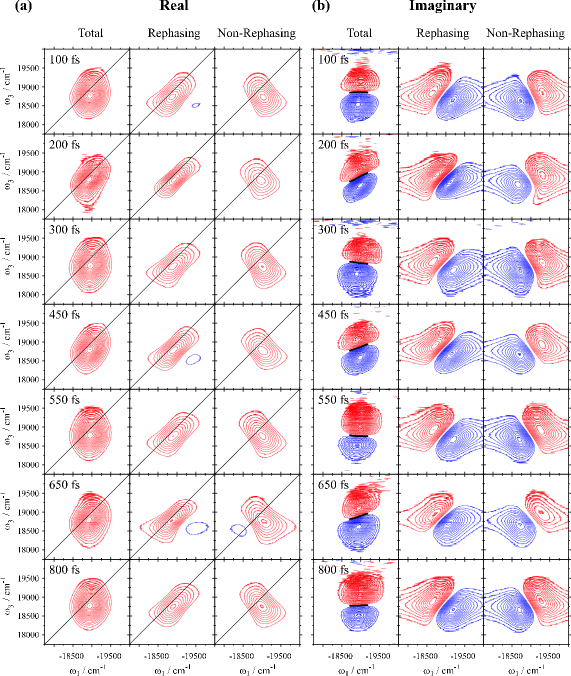
Figure 4: (a) Real and (b) imaginary part of the 2D spectra of PERY in toluene for $t_{2}$-delays of 100, 200, 300, 450, 550, 650, and 800 fs. The first, second, and third column of each panel display the corresponding total signal, the rephasing, and the non-rephasing part, respectively. All total spectra are normalized to their absolute maximum value, whereas the rephasing and non-rephasing parts are plotted with their respective contribution to the total signal. Contour lines are drawn at 5$\%$ intervals starting at $\pm 10\%$. Red lines indicate positive signals, blue lines negative ones. The solid line in the real part indicates the diagonal, whereas the black lines in the imaginary part are drawn at the zero crossings between the positive and negative features.

The real part of a 2D spectrum (first column in Fig. 4a) is the product of absorptive line-shapes in $\omega_{1}$ and in $\omega_{3}$. In agreement with approximating PERY as a two-level electronic system, where ground state bleaching and stimulated emission are the only two contributions, it shows a single positive feature. The maximum of the peak is centered slightly below the diagonal ($|\omega_{1}|>\omega_{3}$), indicative of a small Stokes shift. The peak experiences periodic modulations in its shape with a period of 240 fs (a detailed analysis is presented in Fig. 7). For $t_{2}$-times of 200, 450, and 650 fs, the shape of the absorptive peak is strongly elliptical with the major axis of the ellipse oriented along the diagonal. Contrarily, for $t_{2}=100,300,550$, and 800 fs the absorptive peak adopts a more circular shape and the major axis is oriented nearly parallel to the $\omega_{3}$-axis.

The imaginary part of a 2D spectrum is the product of an absorptive line-shape in $\omega_{1}$ and a dispersive line-shape in $\omega_{3}$. In case of a two-level system the imaginary part features two contributions of opposite sign (first column in Fig. 4b). Similar to the real part, the imaginary part too exhibits oscillations with a period of 240 fs. The most obvious oscillation is seen in the nodal line separating the positive and negative feature. The angle of this nodal line with respect to the $\omega_{1}$-axis changes from being positive for $t_{2}=200$, 450, and 650 fs, to zero or even negative values for $t_{2}=100$, 300, 550, and 800 fs (cf. Fig. 7 for a detailed evaluation). In addition to this oscillation of the nodal line, the width of both contributions periodically changes from being narrow for $t_{2}=200$, 450, and 650 fs, to being broad for $t_{2}=100$, 300, 550, and 800 fs.

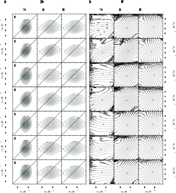
Figure 5: (a) Amplitude and (b) phase of the 2D spectra of PERY in toluene recorded at $t_{2}$-delays of 100, 200, 300, 450, 550, 650, and 800 fs. The first, second, and third column of each panel display the corresponding total signal, the rephasing and the non-rephasing part, respectively. The amplitude part total spectra are normalized to their absolute maximum value, whereas the rephasing and non-rephasing parts are plotted with their respective contribution to the total signal. Contour lines are drawn at 5$\%$ intervals starting at $\pm 10\%$ in the amplitude part spectra and at $\pm\frac{\pi}{12}$ intervals in the phase spectra. The zero-phase line is indicated in each phase spectrum. Note the different spectral range in the representation of the phase spectra.

In Fig. 5 we show amplitude and phase 2D spectra of PERY for $t_{2}$-delays of 100, 200, 300, 450, 550, 650, and 800 fs. The amplitude spectra (first column in Fig. 5a) resemble the real part spectra shown in Fig. 4a, with a single feature centered slightly below the diagonal. Similar to the real part spectra this positive peak features oscillations in its orientation and shape. For $t_{2}=$ 200, 450, and 650 fs the peak shape is highly elliptical and its major axis is oriented along the diagonal. For $t_{2}=$ 100, 300, 550, and 800 fs the peak acquires a more circular shape and is oriented nearly parallel to the $\omega_{3}$-axis.

In the phase spectra (first column in Fig. 5b) the lines of constant phase exhibit oscillations in their orientation. For $t_{2}=$ 200, 450, and 650 fs the lines of constant phase are oriented along the diagonal, whereas they turn to become horizontal at $t_{2}=$ 100, 300, 550, and 800 fs. Note that the phase spectra are shown for a narrower range than the real, imaginary, and amplitude part spectra. All the observed line-shape modulations will be assigned below to periodic modulations in the strength of the rephasing and non-rephasing contributions to the total signal.

IV.2 Rephasing and non-rephasing signal parts

The third-order nonlinear polarization $P^{(3)}(t_{1},t_{2},t_{3})$, which underlies all FWM signals, can be expressed as a convolution of the appropriate response functions $R_{i}(t_{1},t_{2},t_{3})$ with the electric fields of the excitation pulses Mukamel (1995). The four Feynman diagrams graphically illustrating the four response functions for a two-level system within the rotating wave approximation are depicted in Fig. 6. In these diagrams the left and right vertical lines indicate the evolution of the $|ket\rangle$ and $\langle bra|$ of the density matrix, respectively. Wavy arrows denote interactions with the electromagnetic field, and time evolves from bottom to top. In all four diagrams, the first interaction of the laser field with the molecular system induces a coherence between the ground state ($g$) and the first excited state ($e$) in which the system evolves for a time $t_{1}$. Interaction with the second laser pulse creates a population or vibrational coherence in either the ground (diagrams $R_{3}$ and $R_{4}$) or the excited (diagrams $R_{1}$ and $R_{2}$) state. After a time $t_{2}$ the third pulse again induces a coherence between the ground and excited state that radiates the signal field in the phase-matched direction $\mathbf{k_{s}}$.

Figure 6: The four Feynman diagrams graphically illustrating the Liouville space pathways for a two-level system within the rotating wave approximation. g and e denote ground and excited state, respectively.

The four Feynman-diagrams shown in Fig. 6 can be classified as ground state bleaching (GSB) and stimulated emission (SE), depending on whether the system evolves in the ground state ($R_{3}$, $R_{4}$) or in the excited state ($R_{1}$, $R_{2}$) during $t_{2}$, respectively. A different classification of these four diagrams arises from the ordering of the first two interactions. In diagrams $R_{2}$ and $R_{3}$ the first interaction takes place with pulse $\mathbf{-k_{1}}$, whereas in diagrams $R_{1}$ and $R_{4}$ the first interaction takes place with positive sign ($\mathbf{+k_{1}}$). As a consequence the system evolves in conjugate frequencies during $t_{1}$ ($\omega_{ge}$) and $t_{3}$ ($\omega_{eg}$) in diagrams $R_{2}$ and $R_{3}$. This allows for rephasing in an inhomogeneously broadened ensemble, resulting in the formation of an "echo" in case the system has kept some memory of its transition frequency over $t_{2}$. These diagrams therefore contribute to the rephasing signal part. In contrast, the system evolves with the same frequency during $t_{1}$ and $t_{3}$ ($\omega_{eg}$) in diagrams $R_{1}$ and $R_{4}$. These two diagrams are denoted non-rephasing and the systems’s response is close to a free induction decay. Rephasing diagrams contribute to the signal for positive delays $t_{1}$ (i.e. pulse 1 preceding pulse 2), whereas non-rephasing diagrams contribute for negative delays of $t_{1}$ (i.e. pulse 2 preceding pulse 1). In addition to these four diagrams there are diagrams that contribute to the signal only if the pulse separation is shorter than the pulse duration, i.e. when the excitation pulses overlap. These diagrams will not be taken into account in our discussion.

Scanning $t_{1}$ over positive and negative values equally weights rephasing and non-rephasing pathways. This scanning procedure has been shown to produce purely absorptive real parts and purely dispersive imaginary parts, that are linked via the Kramers-Kronig relation Hybl et al. (2001a); Khalil et al. (2003a). The rephasing and non-rephasing spectra on their own exhibit phase-twisted line-shapes resulting from mixing of dispersive and absorptive features. The dissection of the total 2D spectrum into its corresponding rephasing and non-rephasing parts is shown in the second and third row of Figs. 4 and 5 for the real part, imaginary part, amplitude, and phase, respectively. The decomposition was performed by recording the full scan and evaluating only positive $t_{1}$-values for the rephasing part and only negative $t_{1}$-values for the non-rephasing part Rem . Strictly speaking, rephasing signals show up at {$-\omega_{1},+\omega_{3}$} according to the conjugate frequency evolution during $t_{1}$ and $t_{3}$. Non-rephasing signals on the other hand appear at {$+\omega_{1},+\omega_{3}$}, since the system evolves with the same frequency during $t_{1}$ and $t_{3}$. However, to facilitate comparison of the rephasing, non-rephasing, and total spectra, we plot all signals along {$-\omega_{1},+\omega_{3}$} Ge et al. (2002); Khalil et al. (2003b).

From the inspection of Fig. 4a, one can immediately see that both rephasing and non-rephasing parts of the real part 2D spectra are of a pronounced elliptical shape. However, the major axis of the ellipse in case of the rephasing part is oriented along the diagonal, whereas it is oriented along the anti-diagonal in case of the non-rephasing part. Each part on its own exhibits oscillations of its amplitude without significant line-shape modulations. The amplitude oscillations, however, are out of phase by $\pi$, i.e. the rephasing part has its maxima at $t_{2}$-times of 200, 450 and 650 fs, whereas the non-rephasing part has its maximal amplitude at $t_{2}=100$, 300, 550, and 800 fs. Therefore, for $t_{2}$-times of 200, 450, and 650 fs the major contribution to the total signal stems from the rephasing part, whereas for $t_{2}$-times of 100, 300, 550, and 800 fs the non-rephasing part contributes more strongly to the total spectrum. In Fig. 7 we present a quantitative evaluation of the respective contributions.

An analogous situation is encountered in the imaginary part as shown in Fig. 4b. The nodal line of the rephasing part is oriented along the diagonal, whereas the one of the non-rephasing part is oriented along the anti-diagonal. As a consequence of the out-of-phase oscillations of the amplitudes of the two contributions, the nodal line of the total signal experiences a periodic modulation of its orientation. Similar to the real part, the rephasing and non-rephasing imaginary peak shapes do not change significantly with increasing $t_{2}$-time, it is only their relative contribution to the total signal that varies with $t_{2}$. From inspection of the dispersive part it becomes most obvious how the phase-twisted line-shapes in the rephasing and non-rephasing signal parts cancel upon summation to yield a purely dispersive imaginary part. In the accompanying paper II we explain the oscillations of the rephasing, nonrephasing, and sum spectra based on an expansion of the frequency-frequency correlation function in terms of Huang-Rhys factors.

The dissection into rephasing and non-rephasing parts was also performed for the amplitude and phase spectra (Fig. 5). For these representations, however, simple addition of the two contributions to yield the total spectrum is not possible. Nevertheless, the oscillations in the total spectra can be assigned to oscillating features in the rephasing and non-rephasing signal parts. In the amplitude part 2D spectra (Fig. 5a), we observe a stronger contribution of the rephasing part for $t_{2}$-delays of 200, 450, and 650 fs, and a reverse situation (i.e. an intensity gain of the non-rephasing contribution) for $t_{2}$-delays of 100, 300, 550, and 800 fs. Therefore, the total signal is elliptical and line-narrowed along the anti-diagonal in the former case, and more circular in the latter. In the phase spectra (Fig. 5b), the lines of constant phase are oriented along the diagonal in the rephasing part and along the anti-diagonal in the non-rephasing part. This behavior reflects the different sign of the phase accumulated during the two time-intervals $t_{1}$ and $t_{3}$ according to the different coherence evolution in the rephasing and non-rephasing Feynman diagrams Loparo et al. (2006). Depending on the relative strength of the rephasing and non-rephasing contributions, lines of constant phase in the total phase spectrum are either oriented along the diagonal ($t_{2}$=200, 450, and 650 fs), or they rotate down to become approximately parallel to the $\omega_{1}$-axis ($t_{2}$=100, 300, 550, and 800 fs). In the next section we discuss relations of the line-shape evolutions in 2D electronic spectra to the frequency-frequency correlation function.

IV.3 Frequency-frequency correlation function

For electronic spectra in the condensed phase, where transition energy fluctuations are non-Markovian in nature, homogeneous and inhomogenous timescales are not readily separable. Therefore, such systems are usually described by a frequency-frequency correlation function (FFCF) $M(t)$, defined as

$$M(t)=\frac{\langle\delta\omega_{eg}(t)\delta\omega_{eg}(0)\rangle}{\langle\delta\omega_{eg}^{2}\rangle}.$$ (2)

$M(t)$ is a normalized ensemble averaged product of transition frequency fluctuations ($\delta\omega_{eg}$) separated by time $t$. Since the correlation function in principle carries all relevant information on intramolecular and system-bath dynamics, considerable attention has been drawn over the last decade on how to sample the FFCF by experimentally feasible methods de Boeij et al. (1996b); Joo et al. (1996); de Boeij et al. (1998). Once $M(t)$ is known, all linear and non-linear spectroscopic signals can be calculated via the line-shape function $g(t)$ with knowledge of the reorganization energy $\lambda$ and the temperature dependent coupling parameter, which reduces to $\frac{2\lambda k_{B}T}{\hbar}$ at high temperatures. We use such complete information about the transition frequency fluctuations due to intramolecular and system bath coupling to derive a detailed line shape theory in Paper II Mančal et al. (2009). Here, we concentrate on the intramolecular part of the $M(t)$-function which is responsible for the oscillatory dynamics of the line shapes.

Although signal detection of one-dimensional FWM signals is relatively straightforward, these methods face an inherent trade-off between time- and frequency-resolution. This obstacle is evaded in 2D-ES, where model calculations and experiments in the IR and VIS spectral region revealed correlations between line-shape evolutions and the frequency-frequency correlation function Hybl et al. (2001b); Woutersen et al. (2002); Khalil et al. (2003b); Kwac and Cho (2003); Roberts et al. (2006); Lazonder et al. (2006); Loparo et al. (2006).

Figure 7: Oscillating features extracted from the 2D spectra of PERY in toluene. (a) Ellipticity (filled circles) and center line slope (open circles) of the peak in the real 2D spectra. (b) Relative amplitudes of the rephasing (filled circles) and the non-rephasing (open circles) part of the real 2D spectra. (c) Inhomogeneity index extracted from the real part 2D spectra as defined in Eq. 4. (d) Slope of the nodal line separating the positive and negative feature in the imaginary 2D spectra. (e) Slope of the $\phi=0$ phase line in the phase 2D spectra.

Two quantities extracted from the real part of 2D electronic spectra were shown to be directly proportional to the FFCF: the ellipticity of the peak shape Lazonder et al. (2006) and the center line slope Kwak et al. (2007); Park et al. (2007). The ellipticity of the peak as a function of $t_{2}$ is defined as Roberts et al. (2006); Lazonder et al. (2006)

$$E(t_{2})=\frac{D^{2}-A^{2}}{D^{2}+A^{2}},$$ (3)

where D and A denote the diagonal and anti-diagonal peak widths, respectively. In Fig. 7a we plot this ratio for $0<t_{2}<800$ fs, with the diagonal and anti-diagonal peak widths evaluated at $\frac{1}{e}$-height. Oscillations with a period of 240 fs are clearly recovered. In our previous work we have shown that these oscillations arise mainly from modulations of the anti-diagonal width, whereas the diagonal width stays nearly constant over the time-range explored in our experiments Nemeth et al. (2008). The center line slope (CLS) is extracted by taking cuts parallel to the $\omega_{3}$-axis and finding the maximum of the peak. The resulting data points as a function of $\omega_{1}$ are fit to a first order polynomial. The slope of this line is the center line slope (Fig. 7a). Note that in the work by Kwak et al. Kwak et al. (2007) cuts are taken parallel to the $\omega_{1}$-axis and the CLS is defined as the inverse of the slope of the line connecting the maxima of the slices. Both the ellipticity and the CLS can vary between 1 and 0 and directly reflect the $t_{2}$-dependent part of the FFCF Lazonder et al. (2006); Kwak et al. (2007) . The limiting value of 1 can be reached for $t_{2}=0$ and in the absence of a homogeneous component. The deviation from the initial value of 1 can thereby be related to the magnitude of the homogeneous component, as was shown in Ref. Kwak et al. (2007). Relaxation and spectral diffusion processes during $t_{2}$ lead to a decrease of the ellipticity and the CLS, until in the long time limit both quantities approach the value of zero, indicative of equal widths along the diagonal and anti-diagonal directions and a slope of the center line that is parallel to the $\omega_{1}$-axis. In a previous work it was argued that the CLS has the advantage over the ellipticity of being independent of factors influencing the line-shape (e.g. finite pulse duration, apodization, etc.) Kwak et al. (2007). As can be seen in Fig. 7a we do not observe significant differences between these two quantities. Closely related to the ellipticity of the peak shape is the eccentricity, which is defined as $Ec=\sqrt{1-\frac{A^{2}}{D^{2}}}$ and which has been proposed in earlier works as a measure for the FFCF Finkelstein et al. (2007). Even though the eccentricity takes the same limiting values as the ellipticity, i.e. 1 if D$>>$A and 0 if D$=$A (which is the case for a circle), the two quantities differ for intermediate cases and therefore cannot be compared directly.

As discussed above, a periodic modulation of the rephasing and non-rephasing contribution to the total 2D spectrum induces the observed changes in the real and imaginary parts. In Fig. 7b we plot the relative amplitudes of the rephasing and non-rephasing part of the real 2D spectra. We clearly observe out-of-phase oscillations of these two contributions, with the rephasing part exhibiting its maxima at $t_{2}$-times of 200, 450, and 650 fs and its minima at $t_{2}=$ 100, 300, 550, and 800 fs, and the non-rephasing part showing the opposite behavior, i.e. having its maxima at $t_{2}$-times corresponding to minima in the rephasing part and vice versa. Tokmakoff et al. Loparo et al. (2006); Roberts et al. (2006) defined an inhomogeneity index $I(t_{2})$ as

$$I(t_{2})=\frac{A_{R}-A_{NR}}{A_{R}+A_{NR}},$$ (4)

with $A_{R}$ being the relative amplitude of the rephasing, and $A_{NR}$ the relative amplitude of the non-rephasing part. This quantity was shown to directly relate to $M(t)$ via $M(t_{2})=\sin{(\frac{\pi I}{2})}$. From the inspection of the inhomogeneity index (Fig. 7b) one can notice, that the non-rephasing part exceeds the rephasing part in signal strength around $t_{2}$-delays of 300 and 550 fs. For these delays the inhomogeneity index adopts negative values, which is consistent with negative peak shift values observed in Fig. 8a (cf. Appendix).

In the imaginary part of 2D spectra it is the slope of the nodal line separating the positive and negative contribution that is related to $M(t)$ Kwac and Cho (2003). We extract this slope from our 2D spectra by finding the zero crossing between the positive and negative contribution in the range $-18700$ cm${}^{-1}<\omega_{1}<-19200$ cm^-1 and fitting of the resulting data points with a first order polynomial. The slope of the nodal line oscillates with a period of 240 fs (Fig. 7d). Note that also the slope takes negative values around $t_{2}=300$ and 550 fs. This agrees well with the observation of negative values of the inhomogeneity index (Fig. 7c) and the peak shift (Fig. 8a). In case of a three-level system it is the real part that features two peaks of opposite sign, with the positive one stemming from ground state bleaching and stimulated emission and the negative feature arising from excited state absorption. In this case the slope of the nodal line is extracted from the real part spectra Hybl et al. (2001b); Eaves et al. (2005); Loparo et al. (2006).

Extracting the frequency-frequency correlation function from the phase spectra (Fig. 5b) is done by evaluating the slope of lines of constant phase Roberts et al. (2006); Loparo et al. (2006). In Fig. 7e we plot this slope for $\phi=0$ evaluated in the frequency range $-18500$cm${}^{-1}<\omega_{1}<-19250$ cm^-1. Again, the oscillating pattern exhibits a period of 240 fs with maxima at $t_{2}$-delays of 200, 450, and 650 fs and minima around $t_{2}=$100, 300, 550, and 800 fs. Around 300 and 550 fs the slope of lines of constant phase adopts negative values indicative of a tilt towards the anti-diagonal axis.

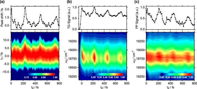
Figure 8: One-dimensional four-wave mixing signals of PERY in toluene. Top and bottom panels share the same abscissa, color scales are shown as insets in the bottom panels. (a) Three-pulse photon echo peak-shift trace (top) and the corresponding frequency integrated three-pulse photon echo signal as a function of delay $t_{1}$ and $t_{2}$. (b) Frequency integrated (top) and frequency resolved (bottom) transient grating signal. (c) Frequency integrated (top) and frequency resolved (bottom) pump-probe signal.

V Conclusion

Intramolecular and system-bath (solvation) dynamics can be studied either in time-domain by the frequency-frequency correlation function $M(t)$, or, equivalently, in frequency-domain by the spectral density $\rho(\omega)$. In this contribution we have concentrated on time-domain measures, by presenting different metrics that can be extracted from two-dimensional electronic spectra and that follow the functional form of the frequency-frequency correlation function. These metrics are the ellipticity, the center line slope, and the inhomogeneity index extracted from the real part spectra, the slope of the nodal line in the imaginary part spectra, and the slope of lines of constant phase in the phase spectra. Peak shift curves of PERY measured in solvents of different polarity (nonpolar, polar, and weakly polar) featured similar timescales Larsen et al. (1999), thus pointing to weak solute-solvent interactions. The observed oscillations in the frequency-frequency correlation function can thus be assumed to be dominated by intramolecular dynamics. The observed beating pattern stems from the fact that during $t_{2}$ the density matrix does not only evolve in a population state (ground or excited state), but vibrational coherences can be excited as well. These coherences evolve with a frequency that is given by the difference in frequency of the two states involved. In theoretical works on vibrational effects in 2D-ES, the vibrational sub-levels could be resolved as a consequence of the customized input parameters Gallagher-Faeder and Jonas (1999); Egorova et al. (2007). Under experimentally feasible conditions effects as finite pulse durations and finite temperature erode the multipeak structure. In such a situation, vibrational dynamics can not be followed by the evolution of diagonal and cross peaks, but by the evolution of line-shapes and signal intensities, as has been done in the present contribution. In our previous work Nemeth et al. (2008) we performed a fit to the experimental two-dimensional spectra by including two overdamped solvent modes and two underdamped intramolecular modes. In the second paper of this series we investigate the influence of vibrational coupling on 2D electronic spectra more thoroughly by employing nonlinear response function theory and expanding the frequency-frequency correlation function in terms of Huang-Rhys factors. Furthermore, we extend the theory also to the case of high frequency modes in which case individual diagonal and cross peaks can be distinguished.

Acknowledgements. This work was supported by the Austrian Science Foundation (FWF) within the projects No. P18233 and F016/18 Advanced Light Sources (ADLIS). A.N. and J.S. thank the Austrian Academy of Sciences for partial financial support by the Doctoral Scholarship Programs (DOCfFORTE and DOC). T. M. acknowledges the kind support by the Czech Science Foundation through grant GACR 202/07/P278 and by the Ministry of Education, Youth, and Sports of the Czech Republic through research plan MSM0021620835. J. H. gratefully acknowledges support by the Lise Meitner project M1080-N16. The quantum-chemical calculations were performed in part on the Schrödinger III cluster at the University of Vienna.

Supplemental Material. The Cartesian B3LYP/SV(P) coordinates, total electronic energy, harmonic vibrational spectrum, Huang-Rhys factors, and a visualisation of the most dominant vibrational modes of PERY can be found in the supplemental material.

Appendix A Comparison to other four-wave mixing signals

Heterodyned two-dimensional electronic spectroscopy gathers the maximum amount of information that can be inferred by any third-order nonlinear technique. Nevertheless it is instructive to cross-check our findings against results that are obtained with alternative detection schemes, shown in Fig. 8. From the experimental point of view, these signals may be differentiated by the required measuring (scanning) time and set-up complexity, while, on the other hand, all of them are related to the functional form of $M(t)$ de Boeij et al. (1996a); Joo et al. (1996); de Boeij et al. (1998).

The three-pulse photon echo peak-shift (3PEPS) method is a variant of homodyned photon echo spectroscopy, in which the time-integrated nonlinear signal

$$S_{3PE}(t_{1},t_{2})=\int_{0}^{\infty}|P^{(3)}(t_{1},t_{2},t_{3})|^{2}\textrm{d}t_{3}$$ (5)

is recorded in a wavevector architecture equivalent to 2D-ES. In each step of a 3PEPS sequence, delay $t_{1}$ is scanned at a fixed delay $t_{2}$, and the position of the (time- and frequency-integrated) signal maximum evaluated along the $t_{1}$-axis. The magnitude of this peak-shift (deviation from $t_{1}=0$) is recorded for a range of $t_{2}$-delays, to give the peak-shift decay. In essence, a finite photon echo peak-shift value indicates the system’s ability to rephase a macroscopic coherence (i.e. to cause an echo) after having spent a certain time ($t_{2}$) in an intermediate state. Fig. 8a shows the photon echo peak-shift decay for PERY in toluene, along with a two-dimensional plot of $S_{3PE}(t_{1},t_{2})$. Both data representations clearly reveal how the photon echo signal maximum oscillates (along $t_{1}$) as a function of $t_{2}$, the oscillation being observable for $t_{2}$-delays well beyond one picosecond. In the context of our analysis of the 2D electronic spectra of PERY, it is interesting to note that the peak-shift acquires negative values around the minima of the peak-shift trace (located at $t_{2}$-delays around 100, 350, and 600 fs). In other words, the integrated photon echo (recorded as a function of $t_{1}$) may peak at negative $t_{1}$-delays, if non-rephasing signal contributions dominate over rephasing contributions to the total signal. We point out that this finding is consistent with the negative value for the inhomogeneity index and a negative slope of the nodal line in the dispersive 2D signal part, observed at the corresponding $t_{2}$-delays.

For the sake of completeness, Fig. 8b and c show the transient grating (TG) and the pump-probe (PP) signals of PERY, in both frequency integrated and frequency resolved representation. The former method records $S_{3PE}$ as a function of $t_{2}$ for delay $t_{1}$ set to zero (descriptively, the first two excitation pulses form a spatial transmission grating from which the third pulse is scattered off). Note that unlike 3PEPS, TG measurements are sensitive to population decay during $t_{2}$. Time delays are scanned in a similar way in PP measurements (i.e. scanning $t_{2}$ for $t_{1}=0$), however, only two pulses are involved in the experiment, the signal being recorded along the direction of the second pulse. Since the PP signal is generated by two interactions with the first pulse (pump), followed by one interaction with the second pulse (probe), $t_{1}$ is intrinsically zero. Overall, also our TG and PP data-sets do well align with previously published data Larsen et al. (1999, 2001) and our 2D electronic spectra. In both types of signals, strong intensity oscillations with a period of 240 fs (140 cm^-1) can be discerned. The slow decay of the TG signal confirms the absence of any fast population decay channels. In line with the discussion above, the PP signal is dominated by (positive) stimulated emission and ground state bleaching contributions, indicating excited state absorption effects to be negligible on the picosecond timescale investigated here.

References

- Zewail (1993) A. Zewail, J. Phys. Chem. 97, 12427 (1993).
- Fragnito et al. (1989) H. L. Fragnito, J.-Y. Bigot, P. C. Becker, and C. V. Shank, Chem. Phys. Lett. 160, 101 (1989).
- Kobayashi et al. (2001) T. Kobayashi, T. Salto, and H. Ohtani, Nature 414, 531 (2001).
- Larsen et al. (2001) D. S. Larsen, K. Ohta, Q.-H. Xu, M. Cyrier, and G. R. Fleming, J. Chem. Phys. 114, 8008 (2001).
- Becker et al. (1989) P. C. Becker, H. L. Fragnito, J. Y. Bigot, C. H. B. Cruz, R. L. Fork, and C. V. Shank, Phys. Rev. Lett. 63, 505 (1989).
- Schoenlein et al. (1993) R. W. Schoenlein, D. M. Mittleman, J. J. Shiang, A. P. Alivisatos, and C. V. Shank, Phys. Rev. Lett. 70, 1014 (1993).
- de Boeij et al. (1998) W. P. de Boeij, M. S. Pshenichnikov, and D. A. Wiersma, Annu. Rev. Phys. Chem. 49, 99 (1998).
- de Boeij et al. (1996a) W. P. de Boeij, M. S. Pshenichnikov, and D. A. Wiersma, J. Phys. Chem. 100, 11806 (1996a).
- Yan and Mukamel (1990) Y. J. Yan and S. Mukamel, Phys. Rev. A 41, 6485 (1990).
- Pollard et al. (1990) W. T. Pollard, H. L. Fragnito, J.-Y. Bigot, C. V. Shank, and R. A. Mathies, Chem. Phys. Lett. 168, 239 (1990).
- Pollard et al. (1992) W. T. Pollard, S. L. Dexheimer, Q. Wang, L. A. Peteanu, C. V. Shank, and R. A. Mathies, J. Phys. Chem. 96, 6147 (1992).
- Dhar et al. (1994) L. Dhar, J. A. Rogers, and K. A. Nelson, Chem. Rev. 94, 157 (1994).
- Ohta et al. (2001) K. Ohta, D. S. Larsen, M. Yang, and G. R. Fleming, J. Chem. Phys. 114, 8020 (2001).
- Hybl et al. (1998) J. D. Hybl, A. W. Albrecht, S. M. G. Faeder, and D. M. Jonas, Chem. Phys. Lett. 297, 307 (1998).
- Tian et al. (2003) P. Tian, D. Keusters, Y. Suzaki, and W. S. Warren, Science 300, 1553 (2003).
- Cowan et al. (2004) M. L. Cowan, J. P. Ogilvie, and R. J. D. Miller, Chem. Phys. Lett. 386, 184 (2004).
- Brixner et al. (2004) T. Brixner, I. V. Stiopkin, and G. R. Fleming, Opt. Lett. 29, 884 (2004).
- Borca et al. (2005) C. N. Borca, T. Zhang, X. Li, and S. T. Cundiff, Chem. Phys. Lett. 416, 311 (2005).
- Gundogdu et al. (2007) K. Gundogdu, K. W. Stone, D. B. Turner, and K. A. Nelson, Chem. Phys. 341, 89 (2007).
- Nemeth et al. (2008) A. Nemeth, F. Milota, T. Mančal, V. Lukeš, H. F. Kauffmann, and J. Sperling, Chem. Phys. Lett. 459, 94 (2008).
- Milota et al. (2009) F. Milota, J. Sperling, A. Nemeth, T. Mančal, and H. F. Kauffmann, Acc. Chem. Res. 42, 1364 (2009).
- Hybl et al. (2002) J. D. Hybl, A. Yu, D. A. Farrow, and D. M. Jonas, J. Phys. Chem. A 106, 7651 (2002).
- Brixner et al. (2005) T. Brixner, J. Stenger, H. M. Vaswani, M. Cho, R. E. Blankenship, and G. R. Fleming, Nature 434, 625 (2005).
- Stiopkin et al. (2006) I. Stiopkin, T. Brixner, M. Yang, and G. R. Fleming, J. Phys. Chem. B 110, 20032 (2006).
- Nemeth et al. (2009) A. Nemeth, V. Lukeš, J. Sperling, F. Milota, H. F. Kauffmann, and T. Mančal, Phys. Chem. Chem. Phys. 11 (2009).
- Pisliakov et al. (2006) A. V. Pisliakov, T. Mančal, and G. R. Fleming, J. Chem. Phys. 124, 234505 (2006).
- Cheng and Fleming (2008) Y.-C. Cheng and G. R. Fleming, J. Phys. Chem. A 112, 4254 (2008).
- Cheng et al. (2007) Y.-C. Cheng, G. S. Engel, and G. R. Fleming, Chem. Phys. 341, 285 (2007).
- Engel et al. (2007) G. S. Engel, T. R. Calhoun, E. L. Read, T.-K. Ahn, T. Mančal, Y.-C. Cheng, R. E. Blankenship, and G. R. Fleming, Nature 446, 782 (2007).
- Milota et al. (2009) F. Milota, J. Sperling, A. Nemeth, and H. F. Kauffmann, Chem. Phys. 357 (2009).
- Collini and Scholes (2009) E. Collini and G. D. Scholes, Science 323, 369 (2009).
- Gallagher-Faeder and Jonas (1999) S. M. Gallagher-Faeder and D. M. Jonas, J. Phys. Chem. A 103, 10489 (1999).
- Egorova et al. (2007) D. Egorova, M. F. Gelin, and W. Domcke, J. Chem. Phys. 126, 074314 (2007).
- Larsen et al. (1999) D. S. Larsen, K. Ohta, and G. R. Fleming, J. Chem. Phys. 111, 8970 (1999).
- Tekavec et al. (2009) P. F. Tekavec, J. A. Myers, K. L. M. Lewis, and J. P. Ogilvie, Opt. Lett. 34 (2009).
- Mančal et al. (2009) T. Mančal, A. Nemeth, F. Milota, V. Lukeš, H. F. Kauffmann, and J. Sperling, J. Chem. Phys. xx (2010).
- Parr and Yang (1991) R. G. Parr and W. Yang, Density-Functional Theory of Atoms and Molecules in Chemistry (Springer, New York, 1991).
- Becke (1996) A. D. Becke, J. Chem. Phys. 104, 1040 (1996).
- Dunning and Hay (1977) T. H. Dunning and P. J. Hay, Methods of electronic structure Theory (Plenum Press, New York, 1977).
- Foresman et al. (1992) J. B. Foresman, M. Head-Gordon, J. A. Pople, and M. J. Frisch, J. Phys. Chem. 96, 135 (1992).
- Zerner et al. (1980) M. C. Zerner, G. H. Loew, R. F. Kirchner, and U. T. Müller-Westerhoff, J. Am. Chem. Soc. 102, 589 (1980).
- Ahlrichs et al. (1989) R. Ahlrichs, M. Bär, M. Häser, H. Horn, and C. Kölmel, Chem. Phys. Lett. 162, 165 (1989).
- Thompson (2004) M. A. Thompson, ArgusLab 4.0.1, Planaria Software LLC, Seattle, WA (2004).
- Stewart (Fujitsu Ltd. 2001) J. J. P. Stewart, http://mtzweb.stanford.edu/programs/ documentation/mopac2002/index.html (Fujitsu Ltd. 2001).
- Piel et al. (2006) J. Piel, E. Riedle, L. Gundlach, R. Ernstorfer, and R. Eichberger, Opt. Lett. 31, 1289 (2006).
- Baum and Riedle (2005) P. Baum and E. Riedle, J. Opt. Soc. B 22, 1875 (2005).
- Trebino et al. (1997) R. Trebino, K. W. DeLong, D. N. Fittinghoff, J. N. Sweetser, M. A. Krumbügel, B. A. Richman, and D. J. Kane, Rev. Sci. Instrum. 68, 3277 (1997).
- Moran et al. (2006) A. Moran, J. Maddox, J. Hong, J. Kim, R. Nome, G. Bazan, S. Mukamel, and N. Scherer, J. Chem. Phys 124, 194904 (2006).
- Tauber et al. (2003) M. J. Tauber, R. A. Mathies, X. Chen, and S. E. Bradforth, Rev. Sci. Instrum. 74, 4958 (2003).
- Laimgruber et al. (2006) S. Laimgruber, H. Schachenmayr, B. Schmidt, W. Zinth, and P. Gilch, Appl. Phys. B 85, 557 (2006).
- Lepetit and Joffre (1996) L. Lepetit and M. Joffre, Opt. Lett. 21, 564 (1996).
- Jonas (2003) D. M. Jonas, Annu. Rev. Phys. Chem. 54, 425 (2003).
- Mukamel (1995) S. Mukamel, Principles of Nonlinear Optical Spectroscopy (Oxford University Press, Oxford, 1995).
- Hybl et al. (2001a) J. D. Hybl, A. A. Ferro, and D. M. Jonas, J. Chem. Phys. 115, 6606 (2001a).
- Khalil et al. (2003a) M. Khalil, N. Demirdöven, and A. Tokmakoff, Phys. Rev. Lett. 90, 47401 (2003a).
- (56) We note that is included in the evaluation of both rephasing and non-rephasing parts resulting in only a negligible deviation of the sum from the total spectrum.
- Ge et al. (2002) N.-H. Ge, M. T. Zanni, and R. M. Hochstrasser, J. Phys. Chem. A 106, 962 (2002).
- Khalil et al. (2003b) M. Khalil, N. Demirdöven, and A. Tokmakoff, J. Phys. Chem. A 107, 5258 (2003b).
- Loparo et al. (2006) J. L. Loparo, S. T. Roberts, and A. Tokmakoff, J. Chem. Phys. 125, 194321 (2006).
- de Boeij et al. (1996b) W. P. de Boeij, M. S. Pshenichnikov, and D. A. Wiersma, Chem. Phys. Lett. 253, 53 (1996b).
- Joo et al. (1996) T. Joo, Y. Jia, J.-Y. Yu, M. J. Lang, and G. R. Fleming, J. Chem. Phys. 104, 6089 (1996).
- Hybl et al. (2001b) J. D. Hybl, Y. Christophe, and D. M. Jonas, Chem. Phys. 266, 295 (2001b).
- Woutersen et al. (2002) S. Woutersen, R. Pfister, P. Hamm, Y. Mu, D. S. Kosov, and G. Stock, J. Chem. Phys. 117, 6833 (2002).
- Kwac and Cho (2003) K. Kwac and M. Cho, J. Chem. Phys. 119, 2256 (2003).
- Roberts et al. (2006) S. T. Roberts, J. J. Loparo, and A. Tokmakoff, J. Chem. Phys. 125, 084502 (2006).
- Lazonder et al. (2006) K. Lazonder, M. S. Pshenichnikov, and D. A. Wiersma, Opt. Lett. 31, 3354 (2006).
- Kwak et al. (2007) K. Kwak, S. Par, I. J. Finkelstein, and M. D. Fayer, J. Chem. Phys. 127, 124503 (2007).
- Park et al. (2007) S. Park, K. Kwak, and M. D. Fayer, Laser Phys. Lett. 4, 704 (2007).
- Finkelstein et al. (2007) I. J. Finkelstein, H. Ishikawa, S. Kim, A. M. Massari, and M. D. Fayer, Proc. Nat. Acad. Sci. 104, 2637 (2007).
- Eaves et al. (2005) J. D. Eaves, J. J. Loparo, C. J. Fecko, S. T. Roberts, A. Tokmakoff, and P. L. Geissler, Proc. Nat. Acad. Sci. 102, 13019 (2005).