Adaptive Submodularity: Theory and Applications in Active Learning and Stochastic Optimization

Abstract

Many problems in artificial intelligence require adaptively making a sequence of decisions with uncertain outcomes under partial observability. Solving such stochastic optimization problems is a fundamental but notoriously difficult challenge. In this paper, we introduce the concept of adaptive submodularity, generalizing submodular set functions to adaptive policies. We prove that if a problem satisfies this property, a simple adaptive greedy algorithm is guaranteed to be competitive with the optimal policy. In addition to providing performance guarantees for both stochastic maximization and coverage, adaptive submodularity can be exploited to drastically speed up the greedy algorithm by using lazy evaluations. We illustrate the usefulness of the concept by giving several examples of adaptive submodular objectives arising in diverse AI applications including management of sensing resources, viral marketing and active learning. Proving adaptive submodularity for these problems allows us to recover existing results in these applications as special cases, improve approximation guarantees and handle natural generalizations.

Keywords: Adaptive Optimization, Stochastic Optimization, Submodularity, Partial Observability, Active Learning, Optimal Decision Trees

1 Introduction

In many problems arising in artificial intelligence one needs to adaptively make a sequence of decisions, taking into account observations about the outcomes of past decisions. Often these outcomes are uncertain, and one may only know a probability distribution over them. Finding optimal policies for decision making in such partially observable stochastic optimization problems is notoriously intractable (see, e.g., Littman et al. (1998)). A fundamental challenge is to identify classes of planning problems for which simple solutions obtain (near-) optimal performance.

In this paper, we introduce the concept of adaptive submodularity, and prove that if a partially observable stochastic optimization problem satisfies this property, a simple adaptive greedy algorithm is guaranteed to obtain near-optimal solutions. In fact, under reasonable complexity-theoretic assumptions, no polynomial time algorithm is able to obtain better solutions in general. Adaptive submodularity generalizes the classical notion of submodularity, which has been successfully used to develop approximation algorithms for a variety of non-adaptive optimization problems. Submodularity, informally, is an intuitive notion of diminishing returns, which states that adding an element to a small set helps more than adding that same element to a larger (super-) set. A celebrated result of the work of Nemhauser et al. (1978) guarantees that for such submodular functions, a simple greedy algorithm, which adds the element that maximally increases the objective value, selects a near-optimal set of $k$ elements. Similarly, it is guaranteed to find a set of near-minimal cost that achieves a desired quota of utility (Wolsey, 1982), using near-minimum average time to do so (Streeter and Golovin, 2008). Besides guaranteeing theoretical performance bounds, submodularity allows us to speed up algorithms without loss of solution quality by using lazy evaluations (Minoux, 1978), often leading to performance improvements of several orders of magnitude (Leskovec et al., 2007). Submodularity has been shown to be very useful in a variety of problems in artificial intelligence (Krause and Guestrin, 2009b).

The challenge in generalizing submodularity to adaptive planning — where the action taken in each step depends on information obtained in the previous steps — is that feasible solutions are now policies (decision trees or conditional plans) instead of subsets. We propose a natural generalization of the diminishing returns property for adaptive problems, which reduces to the classical characterization of submodular set functions for deterministic distributions. We show how these results of Nemhauser et al. (1978), Wolsey (1982), Streeter and Golovin (2008), and Minoux (1978) generalize to the adaptive setting. Hence, we demonstrate how adaptive submodular optimization problems enjoy theoretical and practical benefits similar to those of classical, nonadaptive submodular problems. We further demonstrate the usefulness and generality of the concept by showing how it captures known results in stochastic optimization and active learning as special cases, admits tighter performance bounds, leads to natural generalizations and allows us to solve new problems for which no performance guarantees were known.

As a first example, consider the problem of deploying (or controlling) a collection of sensors to monitor some spatial phenomenon. Each sensor can cover a region depending on its sensing range. Suppose we would like to find the best subset of $k$ locations to place the sensors. In this application, intuitively, adding a sensor helps more if we have placed few sensors so far and helps less if we have already placed many sensors. We can formalize this diminishing returns property using the notion of submodularity – the total area covered by the sensors is a submodular function defined over all sets of locations. Krause and Guestrin (2007) show that many more realistic utility functions in sensor placement (such as the improvement in prediction accuracy w.r.t. some probabilistic model) are submodular as well. Now consider the following stochastic variant: Instead of deploying a fixed set of sensors, we deploy one sensor at a time. With a certain probability, deployed sensors can fail, and our goal is to maximize the area covered by the functioning sensors. Thus, when deploying the next sensor, we need to take into account which of the sensors we deployed in the past failed. This problem has been studied by Asadpour et al. (2008) for the case where each sensor fails independently at random. In this paper, we show that the coverage objective is adaptive submodular, and use this concept to handle much more general settings (where, e.g., rather than all-or-nothing failures there are different types of sensor failures of varying severity). We also consider a related problem where the goal is to place the minimum number of sensors to achieve the maximum possible sensor coverage (i.e., the coverage obtained by deploying sensors everywhere), or more generally the goal may be to achieve any fixed percentage of the maximum possible sensor coverage. Under the first goal, the problem is equivalent to one studied by Goemans and Vondrák (2006), and generalizes a problem studied by Liu et al. (2008).

As another example, consider a viral marketing problem, where we are given a social network, and we want to influence as many people as possible in the network to buy some product. We do that by giving the product for free to a subset of the people, and hope that they convince their friends to buy the product as well. Formally, we have a graph, and each edge $e$ is labeled by a number $0\leq p_{e}\leq 1$. We “influence” a subset of nodes in the graph, and for each influenced node, their neighbors get randomly influenced according to the probability annotated on the edge connecting the nodes. This process repeats until no further node gets influenced. Kempe et al. (2003) show that the set function which quantifies the expected number of nodes influenced is submodular. A natural stochastic variant of the problem is where we pick a node, get to see which nodes it influenced, then adaptively pick the next node based on these observations and so on. We show that a large class of such adaptive influence maximization problems satisfies adaptive submodularity.

Our third application is in active learning, where we are given an unlabeled data set, and we would like to adaptively pick a small set of examples whose labels imply all other labels. The same problem arises in automated diagnosis, where we have hypotheses about the state of the system (e.g., what illness a patient has), and would like to perform tests to identify the correct hypothesis. In both domains we want to pick examples / tests to shrink the remaining version space (the set of consistent hypotheses) as quickly as possible. Here, we show that the reduction in version space probability mass is adaptive submodular, and use that observation to prove that the adaptive greedy algorithm is a near-optimal querying policy. Our results for active learning and automated diagnosis are also related to recent results of Guillory and Bilmes (2010); Guillory and Bilmes (2011) who study generalizations of submodular set cover to an interactive setting. In contrast to our approach however, Guillory and Bilmes analyze worst-case costs, and use rather different technical definitions and proof techniques.

We summarize our main contributions below, and provide a more technical summary in Table 1. At a high level, our main contributions are:

• We consider a particular class of partially observable adaptive stochastic optimization problems, which we prove to be hard to approximate in general.

• We introduce the concept of adaptive submodularity, and prove that if a problem instance satisfies this property, a simple adaptive greedy policy performs near-optimally, for both adaptive stochastic maximization and coverage, and also a natural min-sum objective.

• We show how adaptive submodularity can be exploited by allowing the use of an accelerated adaptive greedy algorithm using lazy evaluations, and how we can obtain data-dependent bounds on the optimum.

• We illustrate adaptive submodularity on several realistic problems, including Stochastic Maximum Coverage, Stochastic Submodular Coverage, Adaptive Viral Marketing, and Active Learning. For these applications, adaptive submodularity allows us to recover known results and prove natural generalizations.

Name	New Results	Location
A.S. Maximization	Tight $(1-1/e)$-approx. for A.M.S. objectives	§5.1, page 5.1
A.S. Min Cost Coverage	Squared logarithmic approx. for A.M.S. objectives	§5.2, page 5.2
A.S. Min Sum Cover	Tight $4$-approx. for A.M.S. objectives	§5.3, page 5.3
Data Dependent Bounds	Generalization to A.M.S. functions	§5.1, page 5.1
Accelerated Greedy	Generalization of lazy evaluations to the adaptive setting	§4, page 4
Stochastic Submodular Maximization	Generalization of the previous $(1-1/e)$-approx. to arbitrary per–item set distributions, and to item costs	§6, page 6
Stochastic Set Cover	$(\ln(n)+1)^{2}$-approx. for arbitrary per-item set distributions, with item costs	§7, page 7
Adaptive Viral Marketing	Adaptive analog of previous $(1-1/e)$-approx. for non-adaptive viral marketing, under more general reward functions; squared logarithmic approx. for the adaptive min cost cover version	§8, page 8
Active Learning	New analysis for generalized binary search and its approximate versions with and without item costs	§9, page 9
Hardness in the absence of Adapt. Submodularity	$\Omega(|E|^{1-\epsilon})$-approximation hardness for A.S. Maximization, Min Cost Coverage, and Min-Sum Cover, if $f$ is not adaptive submodular.	§12, page 12

Table 1: Summary of our theoretical results. A.S. is shorthand for “adaptive stochastic”, and A.M.S. is shorthand for “adaptive monotone submodular.”

1.1 Organization

This article is organized as follows. In §2 (page 2) we set up notation and formally define the relevant adaptive optimization problems for general objective functions. For the reader’s convenience, we have also provided a reference table of important symbols on page 2. In §3 (page 3) we review the classical notion of submodularity and introduce the novel adaptive submodularity property. In §4 (page 4) we introduce the adaptive greedy policy, as well as an accelerated variant. In §5 (page 5) we discuss the theoretical guarantees that the adaptive greedy policy enjoys when applied to problems with adaptive submodular objectives. Sections 6 through 9 provide examples on how to apply the adaptive submodular framework to various applications, namely Stochastic Submodular Maximization (§6, page 6), Stochastic Submodular Coverage (§7, page 7), Adaptive Viral Marketing (§8, page 8), and Active Learning (§9, page 9). In §10 (page 10) we report empirical results on two sensor selection problems. In §11 (page 11) we discuss the adaptivity gap of the problems we consider, and in §12 (page 12) we prove hardness results indicating that problems which are not adaptive submodular can be extremely inapproximable under reasonable complexity assumptions. We review related work in §13 (page 13) and provide concluding remarks in §14 (page 14). The Appendix (page 15) gives details of how to incorporate item costs and includes all of the proofs omitted from the main text.

2 Adaptive Stochastic Optimization

We start by introducing notation and defining the general class of adaptive optimization problems that we address in this paper. For sake of clarity, we will illustrate our notation using the sensor placement application mentioned in §1. We give examples of other applications in §6, §7, §8, and §9.

2.1 Items and Realizations

Let $E$ be a finite set of items (e.g., sensor locations). Each item $e\in E$ is in a particular (initially unknown) state from a set $O$ of possible states (describing whether a sensor placed at location $e$ would malfunction or not). We represent the item states using a function ${\color[rgb]{0,0,0}{\phi}}:E\rightarrow O$, called a realization (of the states of all items in the ground set). Thus, we say that ${\color[rgb]{0,0,0}{\phi}}(e)$ is the state of $e$ under realization ${\color[rgb]{0,0,0}{\phi}}$. We use ${\color[rgb]{0,0,0}{\Phi}}$ to denote a random realization. We take a Bayesian approach and assume that there is a known prior probability distribution ${\color[rgb]{0,0,0}{p\left({{\color[rgb]{0,0,0}{\phi}}}\right)}}:=\mathbb{P}\left[{\color[rgb]{0,0,0}{\Phi}}={\color[rgb]{0,0,0}{\phi}}\right]$ over realizations (e.g., modeling that sensors fail independently with failure probability), so that we can compute posterior distributions. We will consider problems where we sequentially pick an item $e\in E$, get to see its state ${\color[rgb]{0,0,0}{\Phi}}(e)$, pick the next item, get to see its state, and so on (e.g., place a sensor, see whether it fails, and so on). After each pick, our observations so far can be represented as a partial realization ${\color[rgb]{0,0,0}{\psi}}$, a function from some subset of $E$ (i.e., the set of items that we already picked) to their states (e.g., ${\color[rgb]{0,0,0}{\psi}}$ encodes where we placed sensors and which of them failed). For notational convenience, we sometimes represent ${\color[rgb]{0,0,0}{\psi}}$ as a relation, so that ${\color[rgb]{0,0,0}{\psi}}\subseteq E\times O$ equals $\left\{(e,o):{\color[rgb]{0,0,0}{\psi}}(e)=o\right\}$. We use the notation $\operatorname{dom}({\color[rgb]{0,0,0}{\psi}})=\left\{e:\exists o.(e,o)\in{\color[rgb]{0,0,0}{\psi}}\right\}$ to refer to the domain of ${\color[rgb]{0,0,0}{\psi}}$ (i.e., the set of items observed in ${\color[rgb]{0,0,0}{\psi}}$). A partial realization ${\color[rgb]{0,0,0}{\psi}}$ is consistent with a realization ${\color[rgb]{0,0,0}{\phi}}$ if they are equal everywhere in the domain of ${\color[rgb]{0,0,0}{\psi}}$. In this case we write ${\color[rgb]{0,0,0}{\phi}}\sim{\color[rgb]{0,0,0}{\psi}}$. If ${\color[rgb]{0,0,0}{\psi}}$ and ${\color[rgb]{0,0,0}{\psi}}^{\prime}$ are both consistent with some ${\color[rgb]{0,0,0}{\phi}}$, and $\operatorname{dom}({\color[rgb]{0,0,0}{\psi}})\subseteq\operatorname{dom}({\color[rgb]{0,0,0}{\psi}}^{\prime})$, we say ${\color[rgb]{0,0,0}{\psi}}$ is a subrealization of ${\color[rgb]{0,0,0}{\psi}}^{\prime}$. Equivalently, ${\color[rgb]{0,0,0}{\psi}}$ is a subrealization of ${\color[rgb]{0,0,0}{\psi}}^{\prime}$ if and only if, when viewed as relations, ${\color[rgb]{0,0,0}{\psi}}\subseteq{\color[rgb]{0,0,0}{\psi}}^{\prime}$.

Partial realizations are similar to the notion of “belief states” in Partially Observable Markov Decision Problems (POMDPs), as they encode the effect of all actions taken (items selected) and observations made, and determine our posterior belief about the state of the world (i.e., the state of all items $e$ not yet selected, ${\color[rgb]{0,0,0}{p\left({{\color[rgb]{0,0,0}{\phi}}\mid{\color[rgb]{0,0,0}{\psi}}}\right)}}:=\mathbb{P}\left[{\color[rgb]{0,0,0}{\Phi}}={\color[rgb]{0,0,0}{\phi}}\mid{\color[rgb]{0,0,0}{\Phi}}\sim{\color[rgb]{0,0,0}{\psi}}\right]$).

2.2 Policies

We encode our adaptive strategy for picking items as a policy $\pi$, which is a function from a set of partial realizations to $E$, specifying which item to pick next under a particular set of observations (e.g., $\pi$ chooses the next sensor location given where we have placed sensors so far, and whether they failed or not). We also allow randomized policies that are functions from a set of partial realizations to distributions on $E$, though our emphasis will primarily be on deterministic policies. If ${\color[rgb]{0,0,0}{\psi}}$ is not in the domain of $\pi$, the policy terminates (stops picking items) upon observation of ${\color[rgb]{0,0,0}{\psi}}$. We use $\operatorname{dom}(\pi)$ to denote the domain of $\pi$. Technically, we require that $\operatorname{dom}(\pi)$ be closed under subrealizations. That is, if ${\color[rgb]{0,0,0}{\psi}}^{\prime}\in\operatorname{dom}(\pi)$ and ${\color[rgb]{0,0,0}{\psi}}$ is a subrealization of ${\color[rgb]{0,0,0}{\psi}}^{\prime}$ then ${\color[rgb]{0,0,0}{\psi}}\in\operatorname{dom}(\pi)$. We use the notation $E({\pi},{{\color[rgb]{0,0,0}{\phi}}})$ to refer to the set of items selected by $\pi$ under realization ${\color[rgb]{0,0,0}{\phi}}$. Each deterministic policy $\pi$ can be associated with a decision tree $T^{\pi}$ in a natural way (see Fig. 1 for an illustration). Here, we adopt a policy-centric view that admits concise notation, though we find the decision tree view to be valuable conceptually.

Since partial realizations are similar to POMDP belief states, our definition of policies is similar to the notion of policies in POMDPs, which are usually defined as functions from belief states to actions. We will further discuss the relationship between the stochastic optimization problems considered in this paper and POMDPs in Section 13.

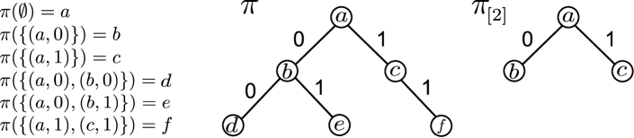
Figure 1: Illustration of a policy $\pi$, its corresponding decision tree representation, and the decision tree representation of $\pi_{[{2}]}$, the level $2$ truncation of $\pi$ (as defined in §5.1).

2.3 Adaptive Stochastic Maximization, Coverage, and Min-Sum Coverage

We wish to maximize, subject to some constraints, a utility function $f:2^{E}\times O^{E}\to\mathbb{R}_{\geq 0}$ that depends on which items we pick and which state each item is in (e.g., modeling the total area covered by the working sensors). Based on this notation, the expected utility of a policy $\pi$ is $f_{\text{avg}}(\pi):=\mathbb{E}\left[f(E({\pi},{{\color[rgb]{0,0,0}{\Phi}}}),{\color[rgb]{0,0,0}{\Phi}})\right]$ where the expectation is taken with respect to ${\color[rgb]{0,0,0}{p\left({{\color[rgb]{0,0,0}{\phi}}}\right)}}$. The goal of the Adaptive Stochastic Maximization problem is to find a policy $\pi^{*}$ such that

$$\pi^{*}\in\mathop{\rm arg\,max}_{\pi}f_{\text{avg}}(\pi)\text{ subject to }|E({\pi},{{\color[rgb]{0,0,0}{\phi}}})|\leq k\text{ for all }{\color[rgb]{0,0,0}{\phi}},$$ (1)

where $k$ is a budget on how many items can be picked (e.g., we would like to adaptively choose $k$ sensor locations such that the working sensors provide as much information as possible in expectation).

Alternatively, we can specify a quota $Q$ of utility that we would like to obtain, and try to find the cheapest policy achieving that quota (e.g., we would like to achieve a certain amount of information, as cheaply as possible in expectation). Formally, we define the average cost ${c_{\text{avg}}{(\pi)}}$ of a policy as the expected number of items it picks, so that ${c_{\text{avg}}{(\pi)}}:=\mathbb{E}\left[|E({\pi},{{\color[rgb]{0,0,0}{\Phi}}})|\right]$. Our goal is then to find

$$\pi^{*}\in\mathop{\rm arg\,min}_{\pi}{c_{\text{avg}}{(\pi)}}\text{ such that }f(E({\pi},{{\color[rgb]{0,0,0}{\phi}}}),{\color[rgb]{0,0,0}{\phi}})\geq Q\text{ for all }{\color[rgb]{0,0,0}{\phi}},$$ (2)

i.e., the policy $\pi^{*}$ that minimizes the expected number of items picked such that under all possible realizations, at least utility $Q$ is achieved. We call Problem 2 the Adaptive Stochastic Minimum Cost Cover problem. We will also consider the problem where we want to minimize the worst-case cost ${c_{\text{wc}}{(\pi)}}:=\max_{{\color[rgb]{0,0,0}{\phi}}}{|E({\pi},{{\color[rgb]{0,0,0}{\phi}}})|}$. This worst-case cost ${c_{\text{wc}}{(\pi)}}$ is the cost incurred under adversarially chosen realizations, or equivalently the depth of the deepest leaf in $T^{\pi}$, the decision tree associated with $\pi$.

Yet another important variant is to minimize the average time required by a policy to obtain its utility. Formally, let $u\!\left({{\pi},{t}}\right)$ be the expected utility obtained by $\pi$ after $t$ steps, let $Q=\mathbb{E}\left[f(E,{\color[rgb]{0,0,0}{\Phi}})\right]$ be the maximum possible expected utility, and define the min-sum cost $c_{\Sigma}\!\left({\pi}\right)$ of a policy as $c_{\Sigma}\!\left({\pi}\right):=\sum_{t=0}^{\infty}\left({Q-u\!\left({{\pi},{t}}\right)}\right)$. We then define the Adaptive Stochastic Min-Sum Cover problem as the search for

$$\pi^{*}\in\mathop{\rm arg\,min}_{\pi}c_{\Sigma}\!\left({\pi}\right).$$ (3)

Unfortunately, as we will show in §12, even for linear functions $f$, i.e., those where $f(A,{\color[rgb]{0,0,0}{\phi}})=\sum_{e\in A}w_{e,{\color[rgb]{0,0,0}{\phi}}}$ is simply the sum of weights (depending on the realization ${\color[rgb]{0,0,0}{\phi}}$), Problems (1), (2), and (3) are hard to approximate under reasonable complexity theoretic assumptions. Despite the hardness of the general problems, in the following sections we will identify conditions that are sufficient to allow us to approximately solve them.

2.4 Incorporating Item Costs

Instead of quantifying the cost of a set $E({\pi},{{\color[rgb]{0,0,0}{\phi}}})$ by the number of elements $|E({\pi},{{\color[rgb]{0,0,0}{\phi}}})|$, we can also consider the case where each item $e\in E$ has a cost $c(e)$, and the cost of a set $S\subseteq E$ is $c(S)=\sum_{e\in S}c(e)$. We can then consider variants of Problems (1), (2), and (3) with the $|E({\pi},{{\color[rgb]{0,0,0}{\phi}}})|$ replaced by $c(E({\pi},{{\color[rgb]{0,0,0}{\phi}}}))$. For clarity of presentation, we will focus on the unit cost case, i.e., $c(e)=1$ for all $e$, and explain how our results generalize to the non-uniform case in the Appendix.

3 Adaptive Submodularity

We first review the classical notion of submodular set functions, and then introduce the novel notion of adaptive submodularity.

3.1 Background on Submodularity

Let us first consider the very special case where ${\color[rgb]{0,0,0}{p\left({{\color[rgb]{0,0,0}{\phi}}}\right)}}$ is deterministic or, equivalently, $|O|=1$ (e.g., in our sensor placement applications, sensors never fail). In this case, the realization ${\color[rgb]{0,0,0}{\phi}}$ is known to the decision maker in advance, and thus there is no benefit in adaptive selection. Given the realization ${\color[rgb]{0,0,0}{\phi}}$, Problem (1) is equivalent to finding a set $A^{*}\subseteq E$ such that

$$A^{*}\in\mathop{\rm arg\,max}_{A\subseteq E}f(A,{\color[rgb]{0,0,0}{\phi}})\text{ such that }|A|\leq k.$$ (4)

For most interesting classes of utility functions $f$, this is an NP-hard optimization problem. However, in many practical problems, such as those mentioned in §1, $f(A)=f(A,{\color[rgb]{0,0,0}{\phi}})$ satisfies submodularity. A set function $f:2^{E}\rightarrow\mathbb{R}$ is called submodular if, whenever $A\subseteq B\subseteq E$ and $e\in E\setminus B$ it holds that

$$f(A\cup\{e\})-f(A)\geq f(B\cup\{e\})-f(B),$$ (5)

i.e., adding $e$ to the smaller set $A$ increases $f$ by at least as much as adding $e$ to the superset $B$. Furthermore, $f$ is called monotone, if, whenever $A\subseteq B$ it holds that $f(A)\leq f(B)$ (e.g., adding a sensor can never reduce the amount of information obtained). A celebrated result by Nemhauser et al. (1978) states that for monotone submodular functions with $f(\emptyset)=0$, a simple greedy algorithm that starts with the empty set, $A_{0}=\emptyset$ and chooses

$$A_{i+1}=A_{i}\cup\{\mathop{\rm arg\,max}_{e\in E\setminus A_{i}}f(A_{i}\cup\{e\})\}$$ (6)

guarantees that $f(A_{k})\geq(1-1/e)\max_{|A|\leq k}f(A)$. Thus, the greedy set $A_{k}$ obtains at least a $(1-1/e)$ fraction of the optimal value achievable using $k$ elements. Furthermore, Feige (1998) shows that this result is tight if $\textrm{P}\neq\textrm{NP}$; under this assumption no polynomial time algorithm can do strictly better than the greedy algorithm, i.e., achieve a $(1-1/e+\epsilon)$-approximation for any constant $\epsilon>0$, even for the special case of Maximum $k$-Cover where $f(A)$ is the cardinality of the union of sets indexed by $A$. Similarly, Wolsey (1982) shows that the same greedy algorithm also near-optimally solves the deterministic case of Problem (2), called the Minimum Submodular Cover problem:

$$A^{*}\in\mathop{\rm arg\,min}_{A\subseteq E}|A|\text{ such that }f(A)\geq Q.$$ (7)

Pick the first set $A_{\ell}$ constructed by the greedy algorithm such that $f(A_{\ell})\geq Q$. Then, for integer-valued submodular functions, $\ell$ is at most $|A^{*}|(1+\log\max_{e}f(e))$, i.e., the greedy set is at most a logarithmic factor larger than the smallest set achieving quota $Q$. For the special case of Set Cover, where $f(A)$ is the cardinality of a union of sets indexed by $A$, this result matches a lower bound by Feige (1998): Unless $\textrm{NP}\subseteq\text{DTIME}(n^{{\mathcal{O}}(\log\log n)})$, Set Cover is hard to approximate by a factor better than $(1-\varepsilon)\ln Q$, where $Q$ is the number of elements to be covered.

Now let us relax the assumption that ${\color[rgb]{0,0,0}{p\left({{\color[rgb]{0,0,0}{\phi}}}\right)}}$ is deterministic. In this case, we may still want to find a non-adaptive solution (i.e., a constant policy $\pi_{A}$ that always picks set $A$ independently of ${\color[rgb]{0,0,0}{\Phi}}$) maximizing $f_{\text{avg}}(\pi_{A})$. If $f$ is pointwise submodular, i.e., $f(A,{\color[rgb]{0,0,0}{\phi}})$ is submodular in $A$ for any fixed ${\color[rgb]{0,0,0}{\phi}}$, the function $f(A)=f_{\text{avg}}(\pi_{A})$ is submodular, since nonnegative linear combinations of submodular functions remain submodular. Thus, the greedy algorithm allows us to find a near-optimal non-adaptive policy. That is, in our sensor placement example, if we are willing to commit to all locations before finding out whether the sensors fail or not, the greedy algorithm can provide a good solution to this non-adaptive problem.

However, in practice, we may be more interested in obtaining a non-constant policy $\pi$, that adaptively chooses items based on previous observations (e.g., takes into account which sensors are working before placing the next sensor). In many settings, selecting items adaptively offers huge advantages, analogous to the advantage of binary search over sequential (linear) search. Thus, the question is whether there is a natural extension of submodularity to policies. In the following, we will develop such a notion – adaptive submodularity.

3.2 Adaptive Monotonicity and Submodularity

The key challenge is to find appropriate generalizations of monotonicity and of the diminishing returns condition (5). We begin by again considering the very special case where ${\color[rgb]{0,0,0}{p\left({{\color[rgb]{0,0,0}{\phi}}}\right)}}$ is deterministic, so that the policies are non-adaptive. In this case a policy $\pi$ simply specifies a sequence of items $(e_{1},e_{2},\ldots,e_{r})$ which it selects in order. Monotonicity in this context can be characterized as the property that “the marginal benefit of selecting an item is always nonnegative,” meaning that for all such sequences $(e_{1},e_{2},\ldots,e_{r})$, items $e$ and $1\leq i\leq r$ it holds that $f(\left\{e_{j}:j\leq i\right\}\cup\{e\})-f(\left\{e_{j}:j\leq i\right\})\geq 0$. Similarly, submodularity can be viewed as the property that “selecting an item later never increases its marginal benefit,” meaning that for all sequences $(e_{1},e_{2},\ldots,e_{r})$, items $e$, and all $i\leq r$, $f(\left\{e_{j}:j\leq i\right\}\cup\left\{e\right\})-f(\left\{e_{j}:j\leq i\right\})\geq f(\left\{e_{j}:j\leq r\right\}\cup\left\{e\right\})-f(\left\{e_{j}:j\leq r\right\})$.

We take these views of monotonicity and submodularity when defining their adaptive analogues, by using an appropriate generalization of the marginal benefit. When moving to the general adaptive setting, the challenge is that the items’ states are now random and only revealed upon selection. A natural approach is thus to condition on observations (i.e., partial realizations of selected items), and take the expectation with respect to the items that we consider selecting. Hence, we define our adaptive monotonicity and submodularity properties in terms of the conditional expected marginal benefit of an item.

Definition 1 (Conditional Expected Marginal Benefit)

Given a partial realization ${\color[rgb]{0,0,0}{\psi}}$ and an item $e$, the conditional expected marginal benefit of $e$ conditioned on having observed ${\color[rgb]{0,0,0}{\psi}}$, denoted $\Delta\left({{e}\!\mid\!{{\color[rgb]{0,0,0}{\psi}}}}\right)$, is

$$\Delta\left({{e}\!\mid\!{{\color[rgb]{0,0,0}{\psi}}}}\right):=\mathbb{E}\left[\frac{}{}\!f(\operatorname{dom}({\color[rgb]{0,0,0}{\psi}})\cup\left\{e\right\},{\color[rgb]{0,0,0}{\Phi}})-f(\operatorname{dom}({\color[rgb]{0,0,0}{\psi}}),{\color[rgb]{0,0,0}{\Phi}})\ \bigg{|}\ {\color[rgb]{0,0,0}{\Phi}}\sim{\color[rgb]{0,0,0}{\psi}}\right]$$ (8)

where the expectation is computed with respect to ${\color[rgb]{0,0,0}{p\left({{\color[rgb]{0,0,0}{\phi}}\mid{\color[rgb]{0,0,0}{\psi}}}\right)}}=\mathbb{P}\left[{\color[rgb]{0,0,0}{\Phi}}={\color[rgb]{0,0,0}{\phi}}\mid{\color[rgb]{0,0,0}{\Phi}}\sim{\color[rgb]{0,0,0}{\psi}}\right]$. Similarly, the conditional expected marginal benefit of a policy $\pi$ is

$$\Delta\left({{\pi}\!\mid\!{{\color[rgb]{0,0,0}{\psi}}}}\right):=\mathbb{E}\left[\frac{}{}\!f(\operatorname{dom}({\color[rgb]{0,0,0}{\psi}})\cup E({\pi},{{\color[rgb]{0,0,0}{\Phi}}}),{\color[rgb]{0,0,0}{\Phi}})-f(\operatorname{dom}({\color[rgb]{0,0,0}{\psi}}),{\color[rgb]{0,0,0}{\Phi}})\ \bigg{|}\ {\color[rgb]{0,0,0}{\Phi}}\sim{\color[rgb]{0,0,0}{\psi}}\right]\mbox{.}$$ (9)

In our sensor placement example, $\Delta\left({{e}\!\mid\!{{\color[rgb]{0,0,0}{\psi}}}}\right)$ quantifies the expected amount of additional area covered by placing a sensor at location $e$, in expectation over the posterior distribution ${\color[rgb]{0,0,0}{p_{{\color[rgb]{0,0,0}{\Phi}}(e)}\!\left({o}\right)}}:=\mathbb{P}\left[{\color[rgb]{0,0,0}{\Phi}}(e)=o\mid{\color[rgb]{0,0,0}{\Phi}}\sim{\color[rgb]{0,0,0}{\psi}}\right]$ of whether the sensor will fail or not, and taking into account the area covered by the placed working sensors as encoded by ${\color[rgb]{0,0,0}{\psi}}$. Note that the benefit we have accrued upon observing ${\color[rgb]{0,0,0}{\psi}}$ (and hence after having selected the items in $\operatorname{dom}({\color[rgb]{0,0,0}{\psi}})$) is $\mathbb{E}\left[f(\operatorname{dom}({\color[rgb]{0,0,0}{\psi}}),{\color[rgb]{0,0,0}{\Phi}})\ \mid\ {\color[rgb]{0,0,0}{\Phi}}\sim{\color[rgb]{0,0,0}{\psi}}\right]$, which is the benefit term subtracted out in Eq. (8) and Eq. (9). Similarly, the expected total benefit obtained after observing ${\color[rgb]{0,0,0}{\psi}}$ and then selecting $e$ is $\mathbb{E}\left[f(\operatorname{dom}({\color[rgb]{0,0,0}{\psi}})\cup\left\{e\right\},{\color[rgb]{0,0,0}{\Phi}})\ \mid\ {\color[rgb]{0,0,0}{\Phi}}\sim{\color[rgb]{0,0,0}{\psi}}\right]$. The corresponding benefit for running $\pi$ after observing ${\color[rgb]{0,0,0}{\psi}}$ is slightly more complex. Under realization ${\color[rgb]{0,0,0}{\phi}}\sim{\color[rgb]{0,0,0}{\psi}}$, the final cumulative benefit will be $f(\operatorname{dom}({\color[rgb]{0,0,0}{\psi}})\cup E({\pi},{{\color[rgb]{0,0,0}{\phi}}}),{\color[rgb]{0,0,0}{\phi}})$. Taking the expectation with respect to ${\color[rgb]{0,0,0}{p\left({{\color[rgb]{0,0,0}{\phi}}\mid{\color[rgb]{0,0,0}{\psi}}}\right)}}$ and subtracting out the benefit already obtained by $\operatorname{dom}({\color[rgb]{0,0,0}{\psi}})$ then yields the conditional expected marginal benefit of $\pi$.

We are now ready to introduce our generalizations of monotonicity and submodularity to the adaptive setting:

Definition 2 (Adaptive Monotonicity)

A function $f:2^{E}\times O^{E}\to\mathbb{R}_{\geq 0}$ is adaptive monotone with respect to distribution ${\color[rgb]{0,0,0}{p\left({{\color[rgb]{0,0,0}{\phi}}}\right)}}$ if the conditional expected marginal benefit of any item is nonnegative, i.e., for all ${\color[rgb]{0,0,0}{\psi}}$ with $\mathbb{P}\left[{\color[rgb]{0,0,0}{\Phi}}\sim{\color[rgb]{0,0,0}{\psi}}\right]>0$ and all $e\in E$ we have

$$\Delta\left({{e}\!\mid\!{{\color[rgb]{0,0,0}{\psi}}}}\right)\geq 0.$$ (10)

Definition 3 (Adaptive Submodularity)

A function $f:2^{E}\times O^{E}\to\mathbb{R}_{\geq 0}$ is adaptive submodular with respect to distribution ${\color[rgb]{0,0,0}{p\left({{\color[rgb]{0,0,0}{\phi}}}\right)}}$ if the conditional expected marginal benefit of any fixed item does not increase as more items are selected and their states are observed. Formally, $f$ is adaptive submodular w.r.t. ${\color[rgb]{0,0,0}{p\left({{\color[rgb]{0,0,0}{\phi}}}\right)}}$ if for all ${\color[rgb]{0,0,0}{\psi}}$ and ${\color[rgb]{0,0,0}{\psi}}^{\prime}$ such that ${\color[rgb]{0,0,0}{\psi}}$ is a subrealization of ${\color[rgb]{0,0,0}{\psi}}^{\prime}$ (i.e., ${\color[rgb]{0,0,0}{\psi}}\subseteq{\color[rgb]{0,0,0}{\psi}}^{\prime}$), and for all $e\in E\setminus\operatorname{dom}({\color[rgb]{0,0,0}{\psi}}^{\prime})$, we have

$$\Delta\left({{e}\!\mid\!{{\color[rgb]{0,0,0}{\psi}}}}\right)\geq\Delta\left({{e}\!\mid\!{{\color[rgb]{0,0,0}{\psi}}^{\prime}}}\right).$$ (11)

From the decision tree perspective, the condition $\Delta\left({{e}\!\mid\!{{\color[rgb]{0,0,0}{\psi}}}}\right)\geq\Delta\left({{e}\!\mid\!{{\color[rgb]{0,0,0}{\psi}}^{\prime}}}\right)$ amounts to saying that for any decision tree $T$, if we are at a node $v$ in $T$ which selects an item $e$, and compare the expected marginal benefit of $e$ selected at $v$ with the expected marginal benefit $e$ would have obtained if it were selected at an ancestor of $v$ in $T$, then the latter must be no smaller than the former. Note that when comparing the two expected marginal benefits, there is a difference in both the set of items previously selected (i.e., $\operatorname{dom}({\color[rgb]{0,0,0}{\psi}})$ vs. $\operatorname{dom}({\color[rgb]{0,0,0}{\psi}}^{\prime})$) and in the distribution over realizations (i.e., ${\color[rgb]{0,0,0}{p\left({{\color[rgb]{0,0,0}{\phi}}\mid{\color[rgb]{0,0,0}{\psi}}}\right)}}$ vs. ${\color[rgb]{0,0,0}{p\left({{\color[rgb]{0,0,0}{\phi}}\mid{\color[rgb]{0,0,0}{\psi}}^{\prime}}\right)}}$). It is also worth emphasizing that adaptive submodularity is defined relative to the distribution ${\color[rgb]{0,0,0}{p\left({{\color[rgb]{0,0,0}{\phi}}}\right)}}$ over realizations; it is possible that $f$ is adaptive submodular with respect to one distribution, but not with respect to another.

We will give concrete examples of adaptive monotone and adaptive submodular functions that arise in the applications introduced in §1 in §6, §7, §8, and §9. In the Appendix, we will explain how the notion of adaptive submodularity can be extended to handle non-uniform costs (since, e.g., the cost of placing a sensor at an easily accessible location may be smaller than at a location that is hard to get to).

3.3 Properties of Adaptive Submodular Functions

It can be seen that adaptive monotonicity and adaptive submodularity enjoy similar closure properties as monotone submodular functions. In particular, if $w_{1},\dots,w_{m}\geq 0$ and $f_{1},\dots,f_{m}$ are adaptive monotone submodular w.r.t. distribution ${\color[rgb]{0,0,0}{p\left({{\color[rgb]{0,0,0}{\phi}}}\right)}}$, then $f(A,{\color[rgb]{0,0,0}{\phi}})=\sum_{i=1}^{m}w_{i}f_{i}(A,{\color[rgb]{0,0,0}{\phi}})$ is adaptive monotone submodular w.r.t. ${\color[rgb]{0,0,0}{p\left({{\color[rgb]{0,0,0}{\phi}}}\right)}}$. Similarly, for a fixed constant $c\geq 0$ and adaptive monotone submodular function $f$, the function $g(E,{\color[rgb]{0,0,0}{\phi}})=\min(f(E,{\color[rgb]{0,0,0}{\phi}}),c)$ is adaptive monotone submodular. Thus, adaptive monotone submodularity is preserved by nonnegative linear combinations and by truncation. Adaptive monotone submodularity is also preserved by restriction, so that if $f:2^{E}\times O^{E}\to\mathbb{R}_{\geq 0}$ is adaptive monotone submodular w.r.t. ${\color[rgb]{0,0,0}{p\left({{\color[rgb]{0,0,0}{\phi}}}\right)}}$, then for any $e\in E$, the function $g:2^{E\setminus\left\{e\right\}}\times O^{E}\to\mathbb{R}_{\geq 0}$ defined by $g(A,{\color[rgb]{0,0,0}{\phi}}):=f(A,{\color[rgb]{0,0,0}{\phi}})$ for all $A\subseteq E\setminus\left\{e\right\}$ and all ${\color[rgb]{0,0,0}{\phi}}$ is also adaptive submodular w.r.t. ${\color[rgb]{0,0,0}{p\left({{\color[rgb]{0,0,0}{\phi}}}\right)}}$. Finally, if $f:2^{E}\times O^{E}\to\mathbb{R}_{\geq 0}$ is adaptive monotone submodular w.r.t. ${\color[rgb]{0,0,0}{p\left({{\color[rgb]{0,0,0}{\phi}}}\right)}}$ then for each partial realization ${\color[rgb]{0,0,0}{\psi}}$ the conditional function $g(A,{\color[rgb]{0,0,0}{\phi}}):=f(A\cup\operatorname{dom}({\color[rgb]{0,0,0}{\psi}}),{\color[rgb]{0,0,0}{\phi}})$ is adaptive monotone submodular w.r.t. ${\color[rgb]{0,0,0}{p\left({{\color[rgb]{0,0,0}{\phi}}\mid{\color[rgb]{0,0,0}{\psi}}}\right)}}:=\mathbb{P}\left[{\color[rgb]{0,0,0}{\Phi}}={\color[rgb]{0,0,0}{\phi}}\mid{\color[rgb]{0,0,0}{\Phi}}\sim{\color[rgb]{0,0,0}{\psi}}\right]$.

3.4 What Problem Characteristics Suggest Adaptive Submodularity?

Adaptive submodularity is a diminishing returns property for policies. Speaking informally, it can be applied in situations where there is an objective function to be optimized does not feature synergies in the benefits of items conditioned on observations. In some cases, the primary objective might not have this property, but a suitably chosen proxy of it does, as is the case with active learning with persistent noise (Golovin et al., 2010; Bellala and Scott, 2010). We give example applications in §6 through §9. It is also worth mentioning where adaptive submodularity is not directly applicable. An extreme example of synergistic effects between items conditioned on observations is the class of “treasure hunting” instances used to prove Theorem 26 on page 26, where the (binary) state of certain groups of items encode the treasure’s location in a complex manner. Another problem feature which adaptive submodularity does not directly address is the possibility that items selection can alter the underlying realization ${\color[rgb]{0,0,0}{\phi}}$, as is the case for the problem of optimizing policies for general POMDPs.

4 The Adaptive Greedy Policy

The classical non-adaptive greedy algorithm (6) has a natural generalization to the adaptive setting. The greedy policy $\pi^{\text{greedy}}$ tries, at each iteration, to myopically increase the expected objective value, given its current observations. That is, suppose $f:2^{E}\times O^{E}\to\mathbb{R}_{\geq 0}$ is the objective, and ${\color[rgb]{0,0,0}{\psi}}$ is the partial realization indicating the states of items selected so far. Then the greedy policy will select the item $e$ maximizing the expected increase in value, conditioned on the observed states of items it has already selected (i.e., conditioned on ${\color[rgb]{0,0,0}{\Phi}}\sim{\color[rgb]{0,0,0}{\psi}}$). That is, it will select $e$ to maximize the conditional expected marginal benefit $\Delta\left({{e}\!\mid\!{{\color[rgb]{0,0,0}{\psi}}}}\right)$ as defined in Eq. (8). Pseudocode of the adaptive greedy algorithm is given in Algorithm 1. The only difference to the classic, non-adaptive greedy algorithm studied by Nemhauser et al. (1978), is Line 1, where an observation ${\color[rgb]{0,0,0}{\Phi}}(e^{*})$ of the selected item $e^{*}$ is obtained. Note that the algorithms in this section are presented for Adaptive Stochastic Maximization. For the coverage objectives, we simply keep selecting items as prescribed by $\pi^{\text{greedy}}$ until achieving the quota on objective value (for the min-cost objective) or until we have selected every item (for the min-sum objective).

4.1 Incorporating Item Costs

The adaptive greedy algorithm can be naturally modified to handle non-uniform item costs by replacing its selection rule by

$$e^{*}\in\mathop{\rm arg\,max}_{e}\frac{\Delta\left({{e}\!\mid\!{{\color[rgb]{0,0,0}{\psi}}}}\right)}{c(e)}.$$

In the following, we will focus on the uniform cost case ($c\equiv 1$), and defer the analysis with costs to the Appendix.

4.2 Approximate Greedy Selection

In some applications, finding an item maximizing $\Delta\left({{e}\!\mid\!{{\color[rgb]{0,0,0}{\psi}}}}\right)$ may be computationally intractable, and the best we can do is find an $\alpha$-approximation to the best greedy selection. This means we find an $e^{\prime}$ such that

$$\Delta\left({{e^{\prime}}\!\mid\!{{\color[rgb]{0,0,0}{\psi}}}}\right)\geq\frac{1}{\alpha}\max_{e}\Delta\left({{e}\!\mid\!{{\color[rgb]{0,0,0}{\psi}}}}\right).$$

We call a policy which always selects such an item an $\alpha$-approximate greedy policy.

Input: Budget $k$; ground set $E$; distribution ${\color[rgb]{0,0,0}{p\left({{\color[rgb]{0,0,0}{\phi}}}\right)}}$; function $f$.

Output: Set $A\subseteq E$ of size $k$

begin AlgoLine0.1$A\leftarrow\emptyset$; ${\color[rgb]{0,0,0}{\psi}}\leftarrow\emptyset$;

AlgoLine0.2 for $i=1$ to $k$ do AlgoLine0.3 foreach $e\in E\setminus A$ do compute $\Delta\left({{e}\!\mid\!{{\color[rgb]{0,0,0}{\psi}}}}\right)=\mathbb{E}\left[f(A\cup\left\{e\right\},{\color[rgb]{0,0,0}{\Phi}})-f(A,{\color[rgb]{0,0,0}{\Phi}})\ |\ {\color[rgb]{0,0,0}{\Phi}}\sim{\color[rgb]{0,0,0}{\psi}}\right]$ ;

AlgoLine0.4Select $e^{*}\in\mathop{\rm arg\,max}_{e}\Delta\left({{e}\!\mid\!{{\color[rgb]{0,0,0}{\psi}}}}\right)$;

AlgoLine0.5Set $A\leftarrow A\cup\{e^{*}\}$;

AlgoLine0.6Observe ${\color[rgb]{0,0,0}{\Phi}}(e^{*})$; Set ${\color[rgb]{0,0,0}{\psi}}\leftarrow{\color[rgb]{0,0,0}{\psi}}\cup\left\{(e^{*},{\color[rgb]{0,0,0}{\Phi}}(e^{*}))\right\}$;

end

Algorithm 1 The adaptive greedy algorithm, which implements the greedy policy.

6

6

6

6

6

6

4.3 Robustness & Approximate Greedy Selection

As we will show, $\alpha$-approximate greedy policies have performance guarantees on several problems. The fact that these performance guarantees of greedy policies are robust to approximate greedy selection suggests a particular robustness guarantee against incorrect priors ${\color[rgb]{0,0,0}{p\left({{\color[rgb]{0,0,0}{\phi}}}\right)}}$. Specifically, if our incorrect prior ${\color[rgb]{0,0,0}{p}}^{\prime}$ is such that when we evaluate $\Delta\left({{e}\!\mid\!{{\color[rgb]{0,0,0}{\psi}}}}\right)$ we err by a multiplicative factor of at most $\alpha$, then when we compute the greedy policy with respect to ${\color[rgb]{0,0,0}{p}}^{\prime}$ we are actually implementing an $\alpha$-approximate greedy policy (with respect to the true prior), and hence obtain the corresponding guarantees. For example, a sufficient condition for erring by at most a multiplicative factor of $\alpha$ is that there exists $c\leq 1$ and $d\geq 1$ with $\alpha=d/c$ such that $c\,{\color[rgb]{0,0,0}{p\left({{\color[rgb]{0,0,0}{\phi}}}\right)}}\leq{\color[rgb]{0,0,0}{p}}^{\prime}\left({{\color[rgb]{0,0,0}{\phi}}}\right)\leq d\,{\color[rgb]{0,0,0}{p\left({{\color[rgb]{0,0,0}{\phi}}}\right)}}$ for all ${\color[rgb]{0,0,0}{\phi}}$, where ${\color[rgb]{0,0,0}{p}}$ is the true prior.

4.4 Lazy Evaluations and the Accelerated Adaptive Greedy Algorithm

The definition of adaptive submodularity allows us to implement an “accelerated” version of the adaptive greedy algorithm using lazy evaluations of marginal benefits as originally suggested for the non-adaptive case by Minoux (1978). The idea is as follows. Suppose we run $\pi^{\text{greedy}}$ under some fixed realization ${\color[rgb]{0,0,0}{\phi}}$, and select items $e_{1},e_{2},\ldots,e_{k}$. Let ${\color[rgb]{0,0,0}{\psi}}_{i}:=\left\{(e_{j},{\color[rgb]{0,0,0}{\phi}}(e_{j}):j\leq i)\right\}$ be the partial realizations observed during the run of $\pi^{\text{greedy}}$. The adaptive greedy algorithm computes $\Delta\left({{e}\!\mid\!{{\color[rgb]{0,0,0}{\psi}}_{i}}}\right)$ for all $e\in E$ and $0\leq i<k$, unless $e\in\operatorname{dom}({\color[rgb]{0,0,0}{\psi}}_{i})$. Naively, the algorithm thus needs to compute $\Theta(|E|k)$ marginal benefits (which can be expensive to compute). The key insight is that $i\mapsto\Delta\left({{e}\!\mid\!{{\color[rgb]{0,0,0}{\psi}}_{i}}}\right)$ is nonincreasing for all $e\in E$, because of the adaptive submodularity of the objective. Hence, if when deciding which item to select as $e_{i}$ we know $\Delta\left({{e^{\prime}}\!\mid\!{{\color[rgb]{0,0,0}{\psi}}_{j}}}\right)\leq\Delta\left({{e}\!\mid\!{{\color[rgb]{0,0,0}{\psi}}_{i}}}\right)$ for some items $e^{\prime}$ and $e$ and $j<i$, then we may conclude $\Delta\left({{e^{\prime}}\!\mid\!{{\color[rgb]{0,0,0}{\psi}}_{i}}}\right)\leq\Delta\left({{e}\!\mid\!{{\color[rgb]{0,0,0}{\psi}}_{i}}}\right)$ and hence eliminate the need to compute $\Delta\left({{e^{\prime}}\!\mid\!{{\color[rgb]{0,0,0}{\psi}}_{i}}}\right)$. The accelerated version of the adaptive greedy algorithm exploits this observation in a principled manner, by computing $\Delta\left({{e}\!\mid\!{{\color[rgb]{0,0,0}{\psi}}}}\right)$ for items $e$ in decreasing order of the upper bounds known on them, until it finds an item whose value is at least as great as the upper bounds of all other items. Pseudocode of this version of the adaptive greedy algorithm is given in Algorithm 2.

In the non-adaptive setting, the use of lazy evaluations has been shown to significantly reduce running times in practice (Leskovec et al., 2007). We evaluated the naive and accelerated implementations of the adaptive greedy algorithm on two sensor selection problems, and obtained speedup factors that range from roughly $4$ to $40$ for those problems. See §10 on page 10 for details.

Input: Budget $k$; ground set $E$; distribution ${\color[rgb]{0,0,0}{p\left({{\color[rgb]{0,0,0}{\phi}}}\right)}}$; function $f$.

Output: Set $A\subseteq E$ of size $k$

begin AlgoLine0.1$A\leftarrow\emptyset$; ${\color[rgb]{0,0,0}{\psi}}\leftarrow\emptyset$; Priority Queue $Q\leftarrow\textsc{empty\_queue}$;

AlgoLine0.2 foreach $e\in E$ do $Q.\operatorname{insert}(e,+\infty)$;

AlgoLine0.3 for $i=1$ to $k$ do AlgoLine0.4$\delta_{\max}\leftarrow-\infty$; $e_{\max}\leftarrow\textsc{null}$;

AlgoLine0.5 while $\delta_{\max}<Q.\operatorname{maxPriority}(\,)$ do AlgoLine0.6$e\leftarrow Q.\operatorname{pop}(\,)$;

AlgoLine0.7$\delta\leftarrow\Delta\left({{e}\!\mid\!{{\color[rgb]{0,0,0}{\psi}}}}\right)=\mathbb{E}\left[f(A\cup\left\{e\right\},{\color[rgb]{0,0,0}{\Phi}})-f(A,{\color[rgb]{0,0,0}{\Phi}})\ |\ {\color[rgb]{0,0,0}{\Phi}}\sim{\color[rgb]{0,0,0}{\psi}}\right]$;

AlgoLine0.8$Q.\operatorname{insert}(e,\delta)$;

AlgoLine0.9if $\delta_{\max}<\delta$ then AlgoLine0.10$\delta_{\max}\leftarrow\delta$; $e_{\max}\leftarrow e$;

AlgoLine0.11$A\leftarrow A\cup\left\{e_{\max}\right\}$; $Q.\operatorname{remove}(e_{\max})$;

AlgoLine0.12Observe ${\color[rgb]{0,0,0}{\Phi}}(e_{\max})$; Set ${\color[rgb]{0,0,0}{\psi}}\leftarrow{\color[rgb]{0,0,0}{\psi}}\cup\left\{(e_{\max},{\color[rgb]{0,0,0}{\Phi}}(e_{\max}))\right\}$;

end

Algorithm 2 The accelerated version of the adaptive greedy algorithm. Here, $Q.\operatorname{insert}(e,\delta)$ inserts $e$ with priority $\delta$, $Q.\operatorname{pop}(\,)$ removes and returns the item with greatest priority, $Q.\operatorname{maxPriority}(\,)$ returns the maximum priority of the elements in $Q$, and $Q.\operatorname{remove}(e)$ deletes $e$ from $Q$.

12

12

12

12

12

12

12

12

12

12

12

12

5 Guarantees for the Greedy Policy

In this section we show that if the objective function is adaptive submodular with respect to the probabilistic model of the environment in which we operate, then the greedy policy inherits precisely the performance guarantees of the greedy algorithm for classic (non-adaptive) submodular maximization and submodular coverage problems, such as Maximum $k$-Cover and Minimum Set Cover, as well as min-sum submodular coverage problems, such as Min-Sum Set Cover. In fact, we will show that this holds true more generally: $\alpha$–approximate greedy policies inherit precisely the performance guarantees of $\alpha$–approximate greedy algorithms for these classic problems. These guarantees suggest that adaptive submodularity is an appropriate generalization of submodularity to policies. In this section we focus on the unit cost case (i.e., every item has the same cost). In the Appendix we provide the proofs omitted in this section, and show how our results extend to non-uniform item costs if we greedily maximize the expected benefit/cost ratio.

5.1 The Maximum Coverage Objective

In this section we consider the maximum coverage objective, where the goal is to select $k$ items adaptively to maximize their expected value. The task of maximizing expected value subject to more complex constraints, such as matroid constraints and intersections of matroid constraints, is considered in the work of Golovin and Krause (2011b). Before stating our result, we require the following definition.

Definition 4 (Policy Truncation)

For a policy $\pi$, define the level-$k$-truncation $\pi_{[{k}]}$ of $\pi$ to be the policy obtained by running $\pi$ until it terminates or until it selects $k$ items, and then terminating. Formally, $\operatorname{dom}(\pi_{[{k}]})=\left\{{\color[rgb]{0,0,0}{\psi}}\in\operatorname{dom}(\pi)\ :\ |{\color[rgb]{0,0,0}{\psi}}|<k\right\}$, and $\pi_{[{k}]}({\color[rgb]{0,0,0}{\psi}})=\pi({\color[rgb]{0,0,0}{\psi}})$ for all ${\color[rgb]{0,0,0}{\psi}}\in\operatorname{dom}(\pi_{[{k}]})$.

We have the following result, which generalizes the classic result of the work of Nemhauser et al. (1978) that the greedy algorithm achieves a $(1-1/e)$-approximation to the problem of maximizing monotone submodular functions under a cardinality constraint. By setting $\ell=k$ and $\alpha=1$ in Theorem 5, we see that the greedy policy which selects $k$ items adaptively obtains at least $(1-1/e)$ of the value of the optimal policy that selects $k$ items adaptively, measured with respect to $f_{\text{avg}}$. For a proof see Theorem 38 in Appendix 15.3, which generalizes Theorem 5 to nonuniform item costs.

Theorem 5

Fix any $\alpha\geq 1$. If $f$ is adaptive monotone and adaptive submodular with respect to the distribution ${\color[rgb]{0,0,0}{p\left({{\color[rgb]{0,0,0}{\phi}}}\right)}}$, and $\pi$ is an $\alpha$-approximate greedy policy, then for all policies $\pi^{*}$ and positive integers $\ell$ and $k$,

$$f_{\text{avg}}(\pi_{[{\ell}]})>\left({1-e^{-\ell/\alpha k}}\right)f_{\text{avg}}(\pi^{*}_{[{k}]})\mbox{.}$$

In particular, with $\ell=k$ this implies any $\alpha$-approximate greedy policy achieves a $\left({1-e^{-1/\alpha}}\right)$ approximation to the expected reward of the best policy, if both are terminated after running for an equal number of steps.

If the greedy rule can be implemented only with small absolute error rather than small relative error, i.e., $\Delta\left({{e^{\prime}}\!\mid\!{{\color[rgb]{0,0,0}{\psi}}}}\right)\geq\max_{e}\Delta\left({{e}\!\mid\!{{\color[rgb]{0,0,0}{\psi}}}}\right)-\varepsilon$, an argument similar to that used to prove Theorem 5 shows that

$$f_{\text{avg}}(\pi_{[{\ell}]})\geq\left({1-e^{-\ell/k}}\right)f_{\text{avg}}(\pi^{*}_{[{k}]})-\ell\varepsilon\mbox{.}$$

This is important, since small absolute error can always be achieved (with high probability) whenever $f$ can be evaluated efficiently, and sampling ${\color[rgb]{0,0,0}{p\left({{\color[rgb]{0,0,0}{\phi}}\mid{\color[rgb]{0,0,0}{\psi}}}\right)}}$ is efficient. In this case, we can approximate

$$\Delta\left({{e}\!\mid\!{{\color[rgb]{0,0,0}{\psi}}}}\right)\approx\frac{1}{N}\sum_{i=1}^{N}\bigl{[}f(\operatorname{dom}({\color[rgb]{0,0,0}{\psi}})\cup\left\{e\right\},{\color[rgb]{0,0,0}{\phi}}_{i})-f(\operatorname{dom}({\color[rgb]{0,0,0}{\psi}}),{\color[rgb]{0,0,0}{\phi}}_{i})\bigr{]}\mbox{,}$$

where ${\color[rgb]{0,0,0}{\phi}}_{i}$ are sampled i.i.d. from ${\color[rgb]{0,0,0}{p\left({{\color[rgb]{0,0,0}{\phi}}\mid{\color[rgb]{0,0,0}{\psi}}}\right)}}$.

5.1.1 Data Dependent Bounds

For the maximum coverage objective, adaptive submodular functions have another attractive feature: they allow us to obtain data dependent bounds on the optimum, in a manner similar to the bounds for the non-adaptive case (Minoux, 1978). Consider the non-adaptive problem of maximizing a monotone submodular function $f:2^{A}\to\mathbb{R}_{\geq 0}$ subject to the constraint $|A|\leq k$. Let $A^{*}$ be an optimal solution, and fix any $A\subseteq E$. Then

$$f(A^{*})\leq f(A)+\max_{B:|B|\leq k}\sum_{e\in B}\left({f(A\cup\left\{e\right\})-f(A)}\right)$$ (12)

because setting $B=A^{*}$ we have $f(A^{*})\leq f(A\cup B)\leq f(A)+\sum_{e\in B}\left({f(A\cup\left\{e\right\})-f(A)}\right)$. Note that unlike the original objective, we can easily compute $\max_{B:|B|\leq k}\sum_{e\in B}\left({f(A\cup\left\{e\right\})-f(A)}\right)$ by computing $\delta(e):=f(A\cup\left\{e\right\})-f(A)$ for each $e$, and summing the $k$ largest values. Hence we can quickly compute an upper bound on our distance from the optimal value, $f(A^{*})-f(A)$. In practice, such data-dependent bounds can be much tighter than the problem-independent performance guarantees of Nemhauser et al. (1978) for the greedy algorithm (Leskovec et al., 2007). Further note that these bounds hold for any set $A$, not just sets selected by the greedy algorithm.

These data dependent bounds have the following analogue for adaptive monotone submodular functions. See Appendix 15.2 for a proof.

Lemma 6 (The Adaptive Data Dependent Bound)

Suppose we have made observations ${\color[rgb]{0,0,0}{\psi}}$ after selecting $\operatorname{dom}({\color[rgb]{0,0,0}{\psi}})$. Let $\pi^{*}$ be any policy such that $|E({\pi^{*}},{{\color[rgb]{0,0,0}{\phi}}})|\leq k$ for all ${\color[rgb]{0,0,0}{\phi}}$. Then for adaptive monotone submodular $f$

$$\Delta\left({{\pi^{*}}\!\mid\!{{\color[rgb]{0,0,0}{\psi}}}}\right)\ \leq\ \max_{A\subseteq E,|A|\leq k}\ \sum_{e\in A}\Delta\left({{e}\!\mid\!{{\color[rgb]{0,0,0}{\psi}}}}\right).$$ (13)

Thus, after running any policy $\pi$, we can efficiently compute a bound on the additional benefit that the optimal solution $\pi^{*}$ could obtain beyond the reward of $\pi$. We do that by computing the conditional expected marginal benefits for all elements $e$, and summing the $k$ largest of them. Note that these bounds can be computed on the fly when running the greedy algorithm, in a similar manner as discussed by Leskovec et al. (2007) for the non-adaptive setting.

5.2 The Min Cost Cover Objective

Another natural objective is to minimize the number of items selected while ensuring that a sufficient level of value is obtained. This leads to the Adaptive Stochastic Minimum Cost Coverage problem described in §2, namely $\pi^{*}\in\mathop{\rm arg\,min}_{\pi}{c_{\text{avg}}{(\pi)}}\text{ such that }f(E({\pi},{{\color[rgb]{0,0,0}{\phi}}}),{\color[rgb]{0,0,0}{\phi}})\geq Q\text{ for all }{\color[rgb]{0,0,0}{\phi}}$. Recall that ${c_{\text{avg}}{(\pi)}}$ is the expected cost of $\pi$, which in the unit cost case equals the expected number of items selected by $\pi$, i.e., ${c_{\text{avg}}{(\pi)}}:=\mathbb{E}\left[|E({\pi},{{\color[rgb]{0,0,0}{\Phi}}})|\right]$. If the objective is adaptive monotone submodular, this is an adaptive version of the Minimum Submodular Cover problem (described on line (7) in §3.1). Recall that the greedy algorithm is known to give a $(\ln(Q)+1)$-approximation for Minimum Submodular Cover assuming the coverage function is integer-valued in addition to being monotone submodular (Wolsey, 1982). Adaptive Stochastic Minimum Cost Coverage is also related to the (Noisy) Interactive Submodular Set Cover problem studied by Guillory and Bilmes (2010); Guillory and Bilmes (2011), which considers the worst-case setting (i.e., there is no distribution over states; instead states are realized in an adversarial manner). Similar results for active learning have been proved by Kosaraju et al. (1999) and Dasgupta (2004), as we discuss in more detail in §9.

We assume throughout this section that there exists a quality threshold $Q$ such that $f(E,{\color[rgb]{0,0,0}{\phi}})=Q$ for all ${\color[rgb]{0,0,0}{\phi}}$, and for all $S\subseteq E$ and all ${\color[rgb]{0,0,0}{\phi}}$, $f(S,{\color[rgb]{0,0,0}{\phi}})\leq Q$. Note that, as discussed in Section 3, if we replace $f(S,{\color[rgb]{0,0,0}{\phi}})$ by a new function $g(S,{\color[rgb]{0,0,0}{\phi}})=\min(f(S,{\color[rgb]{0,0,0}{\phi}}),Q^{\prime})$ for some constant $Q^{\prime}$, $g$ will be adaptive submodular if $f$ is. Thus, if $f(E,{\color[rgb]{0,0,0}{\phi}})$ varies across realizations, we can instead use the greedy algorithm on the function truncated at some threshold $Q^{\prime}\leq\min_{{\color[rgb]{0,0,0}{\phi}}}f(E,{\color[rgb]{0,0,0}{\phi}})$ achievable by all realizations.

In contrast to Adaptive Stochastic Maximization, for the coverage problem additional subtleties arise. In particular, it is not enough that a policy $\pi$ achieves value $Q$ for the true realization; in order for $\pi$ to terminate, it also requires a proof of this fact. Formally, we require that $\pi$ covers $f$:

Definition 7 (Coverage)

Let ${\color[rgb]{0,0,0}{\psi}}={\color[rgb]{0,0,0}{\psi}}(\pi,{\color[rgb]{0,0,0}{\phi}})$ be the partial realization encoding all states observed during the execution of $\pi$ under realization ${\color[rgb]{0,0,0}{\phi}}$. Given $f:2^{E}\times O^{E}\to\mathbb{R}$, we say a policy $\pi$ covers ${\color[rgb]{0,0,0}{\phi}}$ with respect to $f$ if $f(\operatorname{dom}({\color[rgb]{0,0,0}{\psi}}),{\color[rgb]{0,0,0}{\phi}}^{\prime})=f(E,{\color[rgb]{0,0,0}{\phi}}^{\prime})$ for all ${\color[rgb]{0,0,0}{\phi}}^{\prime}\sim{\color[rgb]{0,0,0}{\psi}}$. We say that $\pi$ covers $f$ if it covers every realization with respect to $f$.

Coverage is defined in such a way that upon terminating, $\pi$ might not know which realization is the true one, but has guaranteed that it has achieved the maximum reward in every possible case (i.e., for every realization consistent with its observations). We obtain results for both the average and worst-case cost objectives.

5.2.1 Minimizing the Average Cost

Before presenting our approximation guarantee for the Adaptive Stochastic Minimum Cost Coverage, we introduce a special class of instances, called self–certifying instances. We make this distinction because the greedy policy has stronger performance guarantees for self–certifying instances, and such instances arise naturally in applications. For example, the Stochastic Submodular Cover and Stochastic Set Cover instances in §7, the Adaptive Viral Marketing instances in §8, and the Pool-Based Active Learning instances in §9 are all self–certifying.

Definition 8 (Self–Certifying Instances)

An instance of Adaptive Stochastic Minimum Cost Coverage is self–certifying if whenever a policy achieves the maximum possible value for the true realization it immediately has a proof of this fact. Formally, an instance $(f,{\color[rgb]{0,0,0}{p\left({{\color[rgb]{0,0,0}{\phi}}}\right)}})$ is self–certifying if for all ${\color[rgb]{0,0,0}{\phi}},{\color[rgb]{0,0,0}{\phi}}^{\prime}$, and ${\color[rgb]{0,0,0}{\psi}}$ such that ${\color[rgb]{0,0,0}{\phi}}\sim{\color[rgb]{0,0,0}{\psi}}$ and ${\color[rgb]{0,0,0}{\phi}}^{\prime}\sim{\color[rgb]{0,0,0}{\psi}}$, we have $f(\operatorname{dom}({\color[rgb]{0,0,0}{\psi}}),{\color[rgb]{0,0,0}{\phi}})=f(E,{\color[rgb]{0,0,0}{\phi}})$ if and only if $f(\operatorname{dom}({\color[rgb]{0,0,0}{\psi}}),{\color[rgb]{0,0,0}{\phi}}^{\prime})=f(E,{\color[rgb]{0,0,0}{\phi}}^{\prime})$.

One class of self–certifying instances which commonly arise are those in which $f(A,{\color[rgb]{0,0,0}{\phi}})$ depends only on the state of items in $A$, and in which there is a uniform maximum amount of reward that can be obtained across realizations. Formally, we have the following observation.

Proposition 9

Fix an instance $(f,{\color[rgb]{0,0,0}{p\left({{\color[rgb]{0,0,0}{\phi}}}\right)}})$. If there exists $Q$ such that $f(E,{\color[rgb]{0,0,0}{\phi}})=Q$ for all ${\color[rgb]{0,0,0}{\phi}}$ and there exists some $g:2^{E\times O}\to\mathbb{R}_{\geq 0}$ such that $f(A,{\color[rgb]{0,0,0}{\phi}})=g\left({\left\{(e,{\color[rgb]{0,0,0}{\phi}}(e)):e\in A\right\}}\right)$ for all $A$ and ${\color[rgb]{0,0,0}{\phi}}$, then $(f,{\color[rgb]{0,0,0}{p\left({{\color[rgb]{0,0,0}{\phi}}}\right)}})$ is self–certifying.

Proof  Fix ${\color[rgb]{0,0,0}{\phi}},{\color[rgb]{0,0,0}{\phi}}^{\prime}$, and ${\color[rgb]{0,0,0}{\psi}}$ such that ${\color[rgb]{0,0,0}{\phi}}\sim{\color[rgb]{0,0,0}{\psi}}$ and ${\color[rgb]{0,0,0}{\phi}}^{\prime}\sim{\color[rgb]{0,0,0}{\psi}}$. Assuming the existence of $g$ and treating ${\color[rgb]{0,0,0}{\psi}}$ as a relation, we have $f(\operatorname{dom}({\color[rgb]{0,0,0}{\psi}}),{\color[rgb]{0,0,0}{\phi}})=g({\color[rgb]{0,0,0}{\psi}})=f(\operatorname{dom}({\color[rgb]{0,0,0}{\psi}}),{\color[rgb]{0,0,0}{\phi}}^{\prime})$. Hence $f(\operatorname{dom}({\color[rgb]{0,0,0}{\psi}}),{\color[rgb]{0,0,0}{\phi}})=Q=f(E,{\color[rgb]{0,0,0}{\phi}})$ if and only if $f(\operatorname{dom}({\color[rgb]{0,0,0}{\psi}}),{\color[rgb]{0,0,0}{\phi}}^{\prime})=Q=f(E,{\color[rgb]{0,0,0}{\phi}}^{\prime})$.  

For our results on minimum cost coverage, we also need a stronger monotonicity condition and a stronger submodularity condition:

Definition 10 (Strong Adaptive Monotonicity)

A function $f:2^{E}\times O^{E}\to\mathbb{R}$ is strongly adaptive monotone with respect to ${\color[rgb]{0,0,0}{p\left({{\color[rgb]{0,0,0}{\phi}}}\right)}}$ if, informally “selecting more items never hurts” with respect to the expected reward. Formally, for all ${\color[rgb]{0,0,0}{\psi}}$, all $e\notin\operatorname{dom}({\color[rgb]{0,0,0}{\psi}})$, and all possible outcomes $o\in O$ such that $\mathbb{P}\left[{\color[rgb]{0,0,0}{\Phi}}(e)=o\ \mid\ {\color[rgb]{0,0,0}{\Phi}}\sim{\color[rgb]{0,0,0}{\psi}}\right]>0$, we require

$$\mathbb{E}\left[f(\operatorname{dom}({\color[rgb]{0,0,0}{\psi}}),{\color[rgb]{0,0,0}{\Phi}})\ \mid\ {\color[rgb]{0,0,0}{\Phi}}\sim{\color[rgb]{0,0,0}{\psi}}\right]\leq\mathbb{E}\left[f(\operatorname{dom}({\color[rgb]{0,0,0}{\psi}})\cup\left\{e\right\},{\color[rgb]{0,0,0}{\Phi}})\ \mid\ {\color[rgb]{0,0,0}{\Phi}}\sim{\color[rgb]{0,0,0}{\psi}},{\color[rgb]{0,0,0}{\Phi}}(e)=o\right]\mbox{.}$$ (14)

Strong adaptive monotonicity implies adaptive monotonicity, as the latter means that “selecting more items never hurts in expectation,” i.e.,

$$\mathbb{E}\left[f(\operatorname{dom}({\color[rgb]{0,0,0}{\psi}}),{\color[rgb]{0,0,0}{\Phi}})\ \mid\ {\color[rgb]{0,0,0}{\Phi}}\sim{\color[rgb]{0,0,0}{\psi}}\right]\leq\mathbb{E}\left[f(\operatorname{dom}({\color[rgb]{0,0,0}{\psi}})\cup\left\{e\right\},{\color[rgb]{0,0,0}{\Phi}})\ \mid\ {\color[rgb]{0,0,0}{\Phi}}\sim{\color[rgb]{0,0,0}{\psi}}\right].$$

To define strong adaptive submodularity, we first need the following extension of $\Delta\left({{e}\!\mid\!{{\color[rgb]{0,0,0}{\psi}}}}\right)$:

Definition 11 (Conditional Expected Marginal Benefit (Extended version))

Given partial realizations
${\color[rgb]{0,0,0}{\psi}}\subseteq{\color[rgb]{0,0,0}{\psi}}^{\prime}$, let

$$\Delta\left({{e}\!\mid\!{{\color[rgb]{0,0,0}{\psi}};{\color[rgb]{0,0,0}{\psi}}^{\prime}}}\right):=\mathbb{E}\left[f(\operatorname{dom}({\color[rgb]{0,0,0}{\psi}})\cup\left\{e\right\},{\color[rgb]{0,0,0}{\Phi}})-f(\operatorname{dom}({\color[rgb]{0,0,0}{\psi}}),{\color[rgb]{0,0,0}{\Phi}})\ \bigg{|}\ {\color[rgb]{0,0,0}{\Phi}}\sim{\color[rgb]{0,0,0}{\psi}}^{\prime}\right]$$ (15)

Definition 12 (Strong Adaptive Submodularity)

A function $f:2^{E}\times O^{E}\to\mathbb{R}_{\geq 0}$ is strongly adaptive submodular with respect to distribution ${\color[rgb]{0,0,0}{p\left({{\color[rgb]{0,0,0}{\phi}}}\right)}}$ if it is adaptive submodular and moreover the expected marginal benefit of any fixed item does not increase as more items are selected and their states are observed, conditioned on the (item, observation) pairs. Formally, $f$ is adaptive submodular w.r.t. ${\color[rgb]{0,0,0}{p\left({{\color[rgb]{0,0,0}{\phi}}}\right)}}$ if for all ${\color[rgb]{0,0,0}{\psi}}$ and ${\color[rgb]{0,0,0}{\psi}}^{\prime}$ such that ${\color[rgb]{0,0,0}{\psi}}$ is a subrealization of ${\color[rgb]{0,0,0}{\psi}}^{\prime}$ (i.e., ${\color[rgb]{0,0,0}{\psi}}\subseteq{\color[rgb]{0,0,0}{\psi}}^{\prime}$), and for all $e\in E\setminus\operatorname{dom}({\color[rgb]{0,0,0}{\psi}}^{\prime})$, we have

$$\Delta\left({{e}\!\mid\!{{\color[rgb]{0,0,0}{\psi}};{\color[rgb]{0,0,0}{\psi}}^{\prime}}}\right)\geq\Delta\left({{e}\!\mid\!{{\color[rgb]{0,0,0}{\psi}}^{\prime}}}\right).$$ (16)

In other words, conditioning on ${\color[rgb]{0,0,0}{\psi}}^{\prime}$, adding items $\operatorname{dom}({\color[rgb]{0,0,0}{\psi}}^{\prime})\setminus\operatorname{dom}({\color[rgb]{0,0,0}{\psi}})$ cannot increase the expected marginal benefit of $e$.

A sufficient condition for strong adaptive submodularity with respect to ${\color[rgb]{0,0,0}{p\left({{\color[rgb]{0,0,0}{\phi}}}\right)}}$ is that the function be adaptive submodular and pointwise submodular (i.e., $f(A,{\color[rgb]{0,0,0}{\phi}})$ is submodular in $A$ for any fixed ${\color[rgb]{0,0,0}{\phi}}$), as we prove in Appendix 15.4. It is worth noting that pointwise submodularity is not sufficient to establish adaptive submodularity. A simple counterexample is $f(S,{\color[rgb]{0,0,0}{\phi}})=|\left\{e:e\in S,{\color[rgb]{0,0,0}{\phi}}(e)=1\right\}|$, with ${\color[rgb]{0,0,0}{p\left({{\color[rgb]{0,0,0}{\phi}}}\right)}}=1/2$ if $\forall e\in E,\ {\color[rgb]{0,0,0}{\phi}}(e)=1$ and ${\color[rgb]{0,0,0}{p\left({{\color[rgb]{0,0,0}{\phi}}}\right)}}=1/2$ if $\forall e\in E,\ {\color[rgb]{0,0,0}{\phi}}(e)=0$. In that case, $\Delta\left({{e}\!\mid\!{\emptyset}}\right)=1/2$ yet $\Delta\left({{e}\!\mid\!{\left\{(e^{\prime},1)\right\}}}\right)=1$ for any $e^{\prime}\neq e$.

We now state our main result for the average case cost ${c_{\text{avg}}{(\pi)}}$:

Theorem 13

Suppose $f:2^{E}\times O^{E}\to\mathbb{R}_{\geq 0}$ is strongly adaptive submodular and strongly adaptive monotone with respect to ${\color[rgb]{0,0,0}{p\left({{\color[rgb]{0,0,0}{\phi}}}\right)}}$ and there exists $Q$ such that $f(E,{\color[rgb]{0,0,0}{\phi}})=Q$ for all ${\color[rgb]{0,0,0}{\phi}}$. Let $\eta$ be any value such that $f(S,{\color[rgb]{0,0,0}{\phi}})>Q-\eta$ implies $f(S,{\color[rgb]{0,0,0}{\phi}})=Q$ for all $S$ and ${\color[rgb]{0,0,0}{\phi}}$. Let $\delta=\min_{{\color[rgb]{0,0,0}{\phi}}}{\color[rgb]{0,0,0}{p\left({{\color[rgb]{0,0,0}{\phi}}}\right)}}$ be the minimum probability of any realization. Let $\pi_{\text{avg}}^{*}$ be an optimal policy minimizing the expected number of items selected to guarantee every realization is covered. Let $\pi$ be an $\alpha$-approximate greedy policy with respect to the item costs. Then in general

$${c_{\text{avg}}{(\pi)}}\leq\alpha\,{c_{\text{avg}}{(\pi_{\text{avg}}^{*})}}\left({\ln\left({\frac{Q}{\delta\eta}}\right)+1}\right)^{2}$$

and for self–certifying instances

$${c_{\text{avg}}{(\pi)}}\leq\alpha\,{c_{\text{avg}}{(\pi_{\text{avg}}^{*})}}\left({\ln\left({\frac{Q}{\eta}}\right)+1}\right)^{2}\mbox{.}$$

Note that if $\operatorname{range}(f)\subset\mathbb{Z}$, then $\eta=1$ is a valid choice, so for general and self–certifying instances we have ${c_{\text{avg}}{(\pi)}}\leq\alpha\,{c_{\text{avg}}{(\pi_{\text{avg}}^{*})}}\left({\ln(Q/\delta)+1}\right)^{2}$ and ${c_{\text{avg}}{(\pi)}}\leq\alpha\,{c_{\text{avg}}{(\pi_{\text{avg}}^{*})}}\left({\ln(Q)+1}\right)^{2}$, respectively.

Historical Note:

An earlier version of Theorem 13 claimed logarithmic approximation factors rather than the squared–logarithmic factors present here. Unfortunately, the proof was flawed as pointed out by Nan and Saligrama (2017). Determining whether the logarithmic bounds hold remains an interesting open problem. In particular, it remains open whether ${c_{\text{avg}}{(\pi)}}\leq\alpha\,{c_{\text{avg}}{(\pi_{\text{avg}}^{*})}}\left({\ln\left({\frac{Q}{\delta\eta}}\right)+1}\right)$ for general instances and ${c_{\text{avg}}{(\pi)}}\leq\alpha\,{c_{\text{avg}}{(\pi_{\text{avg}}^{*})}}\left({\ln\left({\frac{Q}{\eta}}\right)+1}\right)$ for self–certifying instances under the conditions specified by Theorem 13. It also remains open whether the strong adaptive submodularity condition is required.

5.2.2 Minimizing the Worst-Case Cost

For the worst-case cost ${c_{\text{wc}}{(\pi)}}:=\max_{{\color[rgb]{0,0,0}{\phi}}}{|E({\pi},{{\color[rgb]{0,0,0}{\phi}}})|}$, strong adaptive monotonicity and strong submodularity are not required; adaptive monotonicity and adaptive submodularity suffice. We obtain the following result.

Theorem 14

Suppose $f:2^{E}\times O^{E}\to\mathbb{R}_{\geq 0}$ is adaptive monotone and adaptive submodular with respect to ${\color[rgb]{0,0,0}{p\left({{\color[rgb]{0,0,0}{\phi}}}\right)}}$, and let $\eta$ be any value such that $f(S,{\color[rgb]{0,0,0}{\phi}})>f(E,{\color[rgb]{0,0,0}{\phi}})-\eta$ implies $f(S,{\color[rgb]{0,0,0}{\phi}})=f(E,{\color[rgb]{0,0,0}{\phi}})$ for all $S$ and ${\color[rgb]{0,0,0}{\phi}}$. Let $\delta=\min_{{\color[rgb]{0,0,0}{\phi}}}{\color[rgb]{0,0,0}{p\left({{\color[rgb]{0,0,0}{\phi}}}\right)}}$ be the minimum probability of any realization. Let $\pi_{wc}^{*}$ be the optimal policy minimizing the worst-case number of queries to guarantee every realization is covered. Let $\pi$ be an $\alpha$-approximate greedy policy. Finally, let $Q:=\mathbb{E}\left[f(E,{\color[rgb]{0,0,0}{\phi}})\right]$ be the maximum possible expected reward. Then

$${c_{\text{wc}}{(\pi)}}\leq\alpha\,{c_{\text{wc}}{(\pi_{wc}^{*})}}\,\left({\ln\left({\frac{Q}{\delta\eta}}\right)+1}\right)\mbox{.}$$

The proofs of Theorems 13 and 14 are given in Appendix 15.4.

Thus, even though adaptive submodularity is defined w.r.t. a particular distribution, perhaps surprisingly, the adaptive greedy algorithm is competitive even in the case of adversarially chosen realizations, against a policy optimized to minimize the worst-case cost. Theorem 14 therefore suggests that if we do not have a strong prior, we can obtain the strongest guarantees if we choose a distribution that is “as uniform as possible” (i.e., maximizes $\delta$) while still guaranteeing adaptive submodularity.

5.2.3 Discussion

Note that the approximation factor for self–certifying instances in Theorem 14 reduces to the $(\ln(Q)+1)$-approximation guarantee for the greedy algorithm for Set Cover instances with $Q$ elements, in the case of a deterministic distribution ${\color[rgb]{0,0,0}{p\left({{\color[rgb]{0,0,0}{\phi}}}\right)}}$. Moreover, with a deterministic distribution ${\color[rgb]{0,0,0}{p\left({{\color[rgb]{0,0,0}{\phi}}}\right)}}$ there is no distinction between average-case and worst-case cost. Hence, an immediate corollary of the result of Feige (1998) mentioned in §3 is that for every constant $\epsilon>0$ there is no polynomial time $(1-\epsilon)\ln\left({Q/\eta}\right)$ approximation algorithm for self–certifying instances of Adaptive Stochastic Min Cost Cover, under either the ${c_{\text{avg}}{(\cdot)}}$ or the ${c_{\text{wc}}{(\cdot)}}$ objective, unless $\textrm{NP}\subseteq\text{DTIME}(n^{{\mathcal{O}}(\log\log n)})$. It remains open to determine whether or not Adaptive Stochastic Min Cost Cover with the worst-case cost objective admits a $\ln\left({Q/\eta}\right)+1$ approximation for self–certifying instances via a polynomial time algorithm, and in particular whether the greedy policy has such an approximation guarantee. However, in Lemma 50 we show that Feige’s result also implies there is no $(1-\epsilon)\ln\left({Q/\delta\eta}\right)$ polynomial time approximation algorithm for general (non self-certifying) instances of Adaptive Stochastic Min Cost Cover under either objective, unless $\textrm{NP}\subseteq\text{DTIME}(n^{{\mathcal{O}}(\log\log n)})$. In that sense, Theorem 14 is best-possible and Theorem 13 cannot be improved by more than a logarithmic factor and under reasonable complexity-theoretic assumptions.

5.3 The Min-Sum Cover Objective

Yet another natural objective is the min-sum objective, in which an unrealized reward of $x$ incurs a cost of $x$ in each time step, and the goal is to minimize the total cost incurred.

5.3.1 Background on the Non-adaptive Min-Sum Cover Problem

In the non-adaptive setting, perhaps the simplest form of a coverage problem with this objective is the Min-Sum Set Cover problem (Feige et al., 2004) in which the input is a set system $(U,{\mathcal{S}})$, the output is a permutation of the sets $\langle S_{1},S_{2},\ldots,S_{m}\rangle$, and the goal is to minimize the sum of element coverage times, where the coverage time of $u$ is the index of the first set that contains it (e.g., it is $j$ if $u\in S_{j}$ and $u\notin S_{i}$ for all $i<j$). In this problem and its generalizations the min-sum objective is useful in modeling processing costs in certain applications, for example in ordering diagnostic tests to identify a disease cheaply (Kaplan et al., 2005), in ordering multiple filters to be applied to database records while processing a query (Munagala et al., 2005), or in ordering multiple heuristics to run on boolean satisfiability instances as a means to solve them faster in practice (Streeter and Golovin, 2008). A particularly expressive generalization of min-sum set cover has been studied under the names Min-Sum Submodular Cover (Streeter and Golovin, 2008) and $L_{1}$-Submodular Set Cover (Golovin et al., 2008). The former paper extends the greedy algorithm to a natural online variant of the problem, while the latter studies a parameterized family of $L_{p}$-Submodular Set Cover problems in which the objective is analogous to minimizing the $L_{p}$ norm of the coverage times for Min-Sum Set Cover instances. In the Min-Sum Submodular Cover problem, there is a monotone submodular function $f:2^{E}\to\mathbb{R}_{\geq 0}$ defining the reward obtained from a collection of elements. There is an integral cost $c(e)$ for each element, and the output is a sequence of all of the elements $\sigma=\langle e_{1},e_{2},\ldots,e_{n}\rangle$. For each $t\in\mathbb{R}_{\geq 0}$, we define the set of elements in the sequence $\sigma$ within a budget of $t$:

$$\sigma_{[{t}]}:=\left\{e_{i}:\sum_{j\leq i}c(e_{j})\leq t\right\}.$$

The cost we wish to minimize is then

$$c_{\Sigma}\!\left({\sigma}\right):=\sum_{t=0}^{\infty}\left({f(E)-f(\sigma_{[{t}]})}\right).$$ (17)

Feige et al. (2004) proved that for Min-Sum Set cover, the greedy algorithm achieves a $4$-approximation to the minimum cost, and also that this is optimal in the sense that no polynomial time algorithm can achieve a $(4-\epsilon)$-approximation, for any $\epsilon>0$, unless $\textrm{P}=\textrm{NP}$. Interestingly, the greedy algorithm also achieves a $4$-approximation for the more general Min-Sum Submodular Cover problem as well (Streeter and Golovin, 2008; Golovin et al., 2008).

5.3.2 The Adaptive Stochastic Min-Sum Cover Problem

In this article, we extend the result of Streeter and Golovin (2008) and Golovin et al. (2008) to an adaptive version of Min-Sum Submodular Cover. For clarity’s sake we will consider the unit-cost case here (i.e., $c(e)=1$ for all $e$); we show how to extend adaptive submodularity to handle general costs in the Appendix. In the adaptive version of the problem, $\pi_{[{t}]}$ plays the role of $\sigma_{[{t}]}$, and $f_{\text{avg}}$ plays the role of $f$. The goal is to find a policy $\pi$ minimizing

$$c_{\Sigma}\!\left({\pi}\right):=\sum_{t=0}^{\infty}\left({\mathbb{E}\left[f(E,{\color[rgb]{0,0,0}{\Phi}})\right]-f_{\text{avg}}(\pi_{[{t}]})}\right)=\sum_{{\color[rgb]{0,0,0}{\phi}}}{\color[rgb]{0,0,0}{p\left({{\color[rgb]{0,0,0}{\phi}}}\right)}}\sum_{t=0}^{\infty}\left({f(E,{\color[rgb]{0,0,0}{\phi}})-f(E(\pi_{[{t}]},{\color[rgb]{0,0,0}{\phi}}),{\color[rgb]{0,0,0}{\phi}})}\right).$$ (18)

We call this problem the Adaptive Stochastic Min-Sum Cover problem. The key difference between this objective and the minimum cost cover objective is that here, the cost at each step is only the fractional extent that we have not covered the true realization, whereas in the minimum cost cover objective we are charged in full in each step until we have completely covered the true realization (according to Definition 7). We prove the following result for the Adaptive Stochastic Min-Sum Cover problem with arbitrary item costs in Appendix 15.5.

Theorem 15

Fix any $\alpha\geq 1$. If $f$ is adaptive monotone and adaptive submodular with respect to the distribution ${\color[rgb]{0,0,0}{p\left({{\color[rgb]{0,0,0}{\phi}}}\right)}}$, $\pi$ is an $\alpha$-approximate greedy policy with respect to the item costs, and $\pi^{*}$ is any policy, then $c_{\Sigma}\!\left({\pi}\right)\leq 4\alpha\,c_{\Sigma}\!\left({\pi^{*}}\right)$.

6 Application: Stochastic Submodular Maximization

As our first application, consider the sensor placement problem introduced in §1. Suppose we would like to monitor a spatial phenomenon such as temperature in a building. We discretize the environment into a set $E$ of locations. We would like to pick a subset $A\subseteq E$ of $k$ locations that is most “informative”, where we use a set function $\hat{f}(A)$ to quantify the informativeness of placement $A$. Krause and Guestrin (2007) show that many natural objective functions (such as reduction in predictive uncertainty measured in terms of Shannon entropy with conditionally independent observations) are monotone submodular.

Now consider the problem, where the informativeness of a sensor is unknown before deployment (e.g., when deploying cameras for surveillance, the location of objects and their associated occlusions may not be known in advance, or varying amounts of noise may reduce the sensing range). We can model this extension by assigning a state ${\color[rgb]{0,0,0}{\phi}}(e)\in O$ to each possible location, indicating the extent to which a sensor placed at location $e$ is working. To quantify the value of a set of sensor deployments under a realization ${\color[rgb]{0,0,0}{\phi}}$ indicating to what extent the various sensors are working, we first define $(e,{o})$ for each $e\in E$ and $o\in O$, which represents the placement of a sensor at location $e$ which is in state $o$. We then suppose there is a function $\hat{f}:2^{E\times O}\to\mathbb{R}_{\geq 0}$ which quantifies the informativeness of a set of sensor deployments in arbitrary states. (Note $\hat{f}$ is a set function taking a set of (sensor deployment, state) pairs as input.) The utility $f(A,{\color[rgb]{0,0,0}{\phi}})$ of placing sensors at the locations in $A$ under realization ${\color[rgb]{0,0,0}{\phi}}$ is then

$$f(A,{\color[rgb]{0,0,0}{\phi}}):=\hat{f}(\left\{(e,{\color[rgb]{0,0,0}{\phi}}(e)):e\in A\right\}).$$

We aim to adaptively place $k$ sensors to maximize our expected utility. We assume that sensor failures at each location are independent of each other, i.e., $\mathbb{P}\left[{\color[rgb]{0,0,0}{\Phi}}={\color[rgb]{0,0,0}{\phi}}\right]=\prod_{e\in E}\mathbb{P}\left[{\color[rgb]{0,0,0}{\Phi}}(e)={\color[rgb]{0,0,0}{\phi}}(e)\right],$ where $\mathbb{P}\left[{\color[rgb]{0,0,0}{\phi}}(e)=o\right]$ is the probability that a sensor placed at location $e$ will be in state $o$. Asadpour et al. (2008) studied a special case of our problem, in which sensors either fail completely (in which case they contribute no value at all) or work perfectly, under the name Stochastic Submodular Maximization. They proved that the adaptive greedy algorithm obtains a $(1-1/e)$ approximation to the optimal adaptive policy, provided $\hat{f}$ is monotone submodular. We extend their result to multiple types of failures by showing that $f(A,{\color[rgb]{0,0,0}{\phi}})$ is adaptive submodular with respect to distribution ${\color[rgb]{0,0,0}{p\left({{\color[rgb]{0,0,0}{\phi}}}\right)}}$ and then invoking Theorem 5. Fig. 2 illustrates an instance of Stochastic Submodular Maximization where $f(A,{\color[rgb]{0,0,0}{\phi}})$ is the cardinality of union of sets index by $A$ and parameterized by ${\color[rgb]{0,0,0}{\phi}}$.

Theorem 16

Fix a prior such that $\mathbb{P}\left[{\color[rgb]{0,0,0}{\Phi}}={\color[rgb]{0,0,0}{\phi}}\right]=\prod_{e\in E}\mathbb{P}\left[{\color[rgb]{0,0,0}{\Phi}}(e)={\color[rgb]{0,0,0}{\phi}}(e)\right]$ and an integer $k$, and let the objective function $\hat{f}:2^{E\times O}\to\mathbb{R}_{\geq 0}$ be monotone submodular. Let $\pi$ be any $\alpha$-approximate greedy policy attempting to maximize $f$, and let $\pi^{*}$ be any policy. Then for all positive integers $\ell$,

$$f_{\text{avg}}(\pi_{[{\ell}]})\geq\left({1-e^{-\ell/\alpha k}}\right)f_{\text{avg}}(\pi^{*}_{[{k}]})\mbox{.}$$

In particular, if $\pi$ is the greedy policy (i.e., $\alpha=1$) and $\ell=k$, then $f_{\text{avg}}(\pi_{[{k}]})\geq\left({1-\frac{1}{e}}\right)f_{\text{avg}}(\pi^{*}_{[{k}]}).$

Proof  We prove Theorem 16 by first proving $f$ is adaptive monotone and adaptive submodular in this model, and then applying Theorem 5. Adaptive monotonicity is readily proved after observing that $f(\cdot,{\color[rgb]{0,0,0}{\phi}})$ is monotone for each ${\color[rgb]{0,0,0}{\phi}}$. Moving on to adaptive submodularity, fix any ${\color[rgb]{0,0,0}{\psi}},{\color[rgb]{0,0,0}{\psi}}^{\prime}$ such that ${\color[rgb]{0,0,0}{\psi}}\subseteq{\color[rgb]{0,0,0}{\psi}}^{\prime}$ and any $e\notin\operatorname{dom}({\color[rgb]{0,0,0}{\psi}}^{\prime})$. We aim to show $\Delta\left({{e}\!\mid\!{{\color[rgb]{0,0,0}{\psi}}^{\prime}}}\right)\leq\Delta\left({{e}\!\mid\!{{\color[rgb]{0,0,0}{\psi}}}}\right)$. Intuitively, this is clear, as $\Delta\left({{e}\!\mid\!{{\color[rgb]{0,0,0}{\psi}}^{\prime}}}\right)$ is the expected marginal benefit of adding $e$ to a larger base set than is the case with $\Delta\left({{e}\!\mid\!{{\color[rgb]{0,0,0}{\psi}}}}\right)$, namely $\operatorname{dom}({\color[rgb]{0,0,0}{\psi}}^{\prime})$ as compared to $\operatorname{dom}({\color[rgb]{0,0,0}{\psi}})$, and the realizations are independent. To prove it rigorously, we define a coupled distribution $\mu$ over pairs of realizations ${\color[rgb]{0,0,0}{\phi}}\sim{\color[rgb]{0,0,0}{\psi}}$ and ${\color[rgb]{0,0,0}{\phi}}^{\prime}\sim{\color[rgb]{0,0,0}{\psi}}^{\prime}$ such that ${\color[rgb]{0,0,0}{\phi}}(e^{\prime})={\color[rgb]{0,0,0}{\phi}}^{\prime}(e^{\prime})$ for all $e^{\prime}\notin\operatorname{dom}({\color[rgb]{0,0,0}{\psi}}^{\prime})$. Formally, $\mu({\color[rgb]{0,0,0}{\phi}},{\color[rgb]{0,0,0}{\phi}}^{\prime})=\prod_{e\in E\setminus\operatorname{dom}({\color[rgb]{0,0,0}{\psi}})}\mathbb{P}\left[{\color[rgb]{0,0,0}{\Phi}}(e)={\color[rgb]{0,0,0}{\phi}}(e)\right]$ if ${\color[rgb]{0,0,0}{\phi}}\sim{\color[rgb]{0,0,0}{\psi}}$, ${\color[rgb]{0,0,0}{\phi}}^{\prime}\sim{\color[rgb]{0,0,0}{\psi}}^{\prime}$, and ${\color[rgb]{0,0,0}{\phi}}(e^{\prime})={\color[rgb]{0,0,0}{\phi}}^{\prime}(e^{\prime})$ for all $e^{\prime}\notin\operatorname{dom}({\color[rgb]{0,0,0}{\psi}}^{\prime})$; otherwise $\mu({\color[rgb]{0,0,0}{\phi}},{\color[rgb]{0,0,0}{\phi}}^{\prime})=0$. (Note that $\mu({\color[rgb]{0,0,0}{\phi}},{\color[rgb]{0,0,0}{\phi}}^{\prime})>0$ implies ${\color[rgb]{0,0,0}{\phi}}(e^{\prime})={\color[rgb]{0,0,0}{\phi}}^{\prime}(e^{\prime})$ for all $e^{\prime}\in\operatorname{dom}({\color[rgb]{0,0,0}{\psi}})$ as well, since ${\color[rgb]{0,0,0}{\phi}}\sim{\color[rgb]{0,0,0}{\psi}}$, ${\color[rgb]{0,0,0}{\phi}}^{\prime}\sim{\color[rgb]{0,0,0}{\psi}}^{\prime}$, and ${\color[rgb]{0,0,0}{\psi}}\subseteq{\color[rgb]{0,0,0}{\psi}}^{\prime}$.) Also note that ${\color[rgb]{0,0,0}{p\left({{\color[rgb]{0,0,0}{\phi}}\mid{\color[rgb]{0,0,0}{\psi}}}\right)}}=\sum_{{\color[rgb]{0,0,0}{\phi}}^{\prime}}\mu({\color[rgb]{0,0,0}{\phi}},{\color[rgb]{0,0,0}{\phi}}^{\prime})$ and ${\color[rgb]{0,0,0}{p\left({{\color[rgb]{0,0,0}{\phi}}^{\prime}\mid{\color[rgb]{0,0,0}{\psi}}^{\prime}}\right)}}=\sum_{{\color[rgb]{0,0,0}{\phi}}}\mu({\color[rgb]{0,0,0}{\phi}},{\color[rgb]{0,0,0}{\phi}}^{\prime})$. Calculating $\Delta\left({{e}\!\mid\!{{\color[rgb]{0,0,0}{\psi}}^{\prime}}}\right)$ and $\Delta\left({{e}\!\mid\!{{\color[rgb]{0,0,0}{\psi}}}}\right)$ using $\mu$, we see that for any $({\color[rgb]{0,0,0}{\phi}},{\color[rgb]{0,0,0}{\phi}}^{\prime})$ in the support of $\mu$,

$$f(\operatorname{dom}({\color[rgb]{0,0,0}{\psi}}^{\prime})\cup\left\{e\right\},{\color[rgb]{0,0,0}{\phi}}^{\prime})-f(\operatorname{dom}({\color[rgb]{0,0,0}{\psi}}^{\prime}),{\color[rgb]{0,0,0}{\phi}}^{\prime}) = \hat{f}({\color[rgb]{0,0,0}{\psi}}^{\prime}\cup\left\{(e,{\color[rgb]{0,0,0}{\phi}}^{\prime}(e))\right\})-\hat{f}({\color[rgb]{0,0,0}{\psi}}^{\prime}))$$

$$\leq \hat{f}({\color[rgb]{0,0,0}{\psi}}\cup\left\{(e,{\color[rgb]{0,0,0}{\phi}}(e))\right\})-\hat{f}({\color[rgb]{0,0,0}{\psi}}))$$

$$= f(\operatorname{dom}({\color[rgb]{0,0,0}{\psi}})\cup\left\{e\right\},{\color[rgb]{0,0,0}{\phi}})-f(\operatorname{dom}({\color[rgb]{0,0,0}{\psi}}),{\color[rgb]{0,0,0}{\phi}})$$

from the submodularity of $\hat{f}$. Hence

$$\begin{array}[]{lllll}\Delta\left({{e}\!\mid\!{{\color[rgb]{0,0,0}{\psi}}^{\prime}}}\right)&=&\sum_{({\color[rgb]{0,0,0}{\phi}},{\color[rgb]{0,0,0}{\phi}}^{\prime})}\mu({\color[rgb]{0,0,0}{\phi}},{\color[rgb]{0,0,0}{\phi}}^{\prime})\left({f(\operatorname{dom}({\color[rgb]{0,0,0}{\psi}}^{\prime})\cup\left\{e\right\},{\color[rgb]{0,0,0}{\phi}}^{\prime})-f(\operatorname{dom}({\color[rgb]{0,0,0}{\psi}}^{\prime}),{\color[rgb]{0,0,0}{\phi}}^{\prime})}\right)&&\\[8.53581pt] &\leq&\sum_{({\color[rgb]{0,0,0}{\phi}},{\color[rgb]{0,0,0}{\phi}}^{\prime})}\mu({\color[rgb]{0,0,0}{\phi}},{\color[rgb]{0,0,0}{\phi}}^{\prime})\left({f(\operatorname{dom}({\color[rgb]{0,0,0}{\psi}})\cup\left\{e\right\},{\color[rgb]{0,0,0}{\phi}})-f(\operatorname{dom}({\color[rgb]{0,0,0}{\psi}}),{\color[rgb]{0,0,0}{\phi}})}\right)&=&\Delta\left({{e}\!\mid\!{{\color[rgb]{0,0,0}{\psi}}}}\right)\end{array}$$

which completes the proof.  

7 Application: Stochastic Submodular Coverage

Suppose that instead of wishing to adaptively place $k$ unreliable sensors to maximize the utility of the information obtained, as discussed in §6, we have a quota on utility and wish to adaptively place the minimum number of unreliable sensors to achieve this quota. This amounts to a minimum-cost coverage version of the Stochastic Submodular Maximization problem introduced in §6, which we call Stochastic Submodular Coverage.

As in §6, in the Stochastic Submodular Coverage problem we suppose there is a function $\hat{f}:2^{E\times O}\to\mathbb{R}_{\geq 0}$ which quantifies the utility of a set of sensors in arbitrary states. Also, the states of each sensor are independent, so that $\mathbb{P}\left[{\color[rgb]{0,0,0}{\Phi}}={\color[rgb]{0,0,0}{\phi}}\right]=\prod_{e\in E}\mathbb{P}\left[{\color[rgb]{0,0,0}{\Phi}}(e)={\color[rgb]{0,0,0}{\phi}}(e)\right]$. The goal is to obtain a quota $Q$ of utility at minimum cost. Thus, we define our objective as $f(A,{\color[rgb]{0,0,0}{\phi}}):=\min\left\{Q,\hat{f}(\left\{(e,{\color[rgb]{0,0,0}{\phi}}(e)):e\in A\right\})\right\}$, and want to find a policy $\pi$ covering every realization and minimizing ${c_{\text{avg}}{(\pi)}}:=\mathbb{E}\left[|E({\pi},{{\color[rgb]{0,0,0}{\Phi}}})|\right]$. We additionally assume that this quota can always be obtained using sufficiently many sensor placements; formally, this amounts to $f(E,{\color[rgb]{0,0,0}{\phi}})=Q$ for all ${\color[rgb]{0,0,0}{\phi}}$. We obtain the following result, whose proof we defer until the end of this section.

Theorem 17

Fix a prior with independent sensor states s.t. $\mathbb{P}\left[{\color[rgb]{0,0,0}{\Phi}}={\color[rgb]{0,0,0}{\phi}}\right]=\prod_{e\in E}\mathbb{P}\left[{\color[rgb]{0,0,0}{\Phi}}(e)={\color[rgb]{0,0,0}{\phi}}(e)\right]$, and let $\hat{f}:2^{E\times O}\to\mathbb{R}_{\geq 0}$ be a mon. submodular function. Fix $Q\in\mathbb{R}_{\geq 0}$ s.t. $f(A,{\color[rgb]{0,0,0}{\phi}}):=\min\left({Q,\ \hat{f}(\left\{(e,{\color[rgb]{0,0,0}{\phi}}(e)):e\in A\right\})}\right)$ satisfies $f(E,{\color[rgb]{0,0,0}{\phi}})=Q$ for all ${\color[rgb]{0,0,0}{\phi}}$. Let $\eta$ be any value such that $f(S,{\color[rgb]{0,0,0}{\phi}})>Q-\eta$ implies $f(S,{\color[rgb]{0,0,0}{\phi}})=Q$ for all $S$ and ${\color[rgb]{0,0,0}{\phi}}$. Finally, let $\pi$ be an $\alpha$-approximate greedy policy for maximizing $f$, and let $\pi^{*}$ be any policy. Then

$${c_{\text{avg}}{(\pi)}}\leq\alpha\,{c_{\text{avg}}{(\pi^{*})}}\left({\ln\left({\frac{Q}{\eta}}\right)+1}\right)^{2}\mbox{.}$$

7.1 A Special Case: The Stochastic Set Coverage Problem

The Stochastic Submodular Coverage problem is a generalization of the Stochastic Set Coverage problem (Goemans and Vondrák, 2006). In Stochastic Set Coverage the underlying submodular objective $\hat{f}$ is the number of elements covered in some input set system. In other words, there is a ground set $U$ of $n$ elements to be covered, and items $E$ such that each item $e$ is associated with a distribution over subsets of $U$. When an item is selected, a set is sampled from its distribution, as illustrated in Fig. 2. The problem is to adaptively select items until all elements of $U$ are covered by sampled sets, while minimizing the expected number of items selected. Like us, Goemans and Vondrák also assume that the subsets are sampled independently for each item, and every element of $U$ can be covered in every realization, so that $f(E,{\color[rgb]{0,0,0}{\phi}})=|U|$ for all ${\color[rgb]{0,0,0}{\phi}}$.

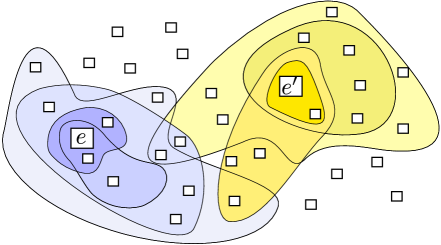
Figure 2: Illustration of part of a Stochastic Set Cover instance. Shown are the supports of two distributions over sets, indexed by items $e$ (marked in blue) and $e^{\prime}$ (yellow).

Goemans and Vondrák primarily investigated the adaptivity gap (quantifying how much adaptive policies can outperform non-adaptive policies) of Stochastic Set Coverage, for variants in which items can be repeatedly selected or not, and prove adaptivity gaps of $\Theta(\log n)$ in the former case, and between $\Omega(n)$ and ${\mathcal{O}}(n^{2})$ in the latter. They also provide an $n$-approximation algorithm. More recently, Liu et al. (2008) considered a special case of Stochastic Set Coverage in which each item may be in one of two states. They were motivated by a streaming database problem, in which a collection of queries sharing common filters must all be evaluated on a stream element. They transform the problem to a Stochastic Set Coverage instance in which (filter, query) pairs are to be covered by filter evaluations; which pairs are covered by a filter depends on the (binary) outcome of evaluating it on the stream element. The resulting instances satisfy the assumption that every element of $U$ can be covered in every realization. They study, among other algorithms, the adaptive greedy algorithm specialized to this setting, and show that if the subsets are sampled independently for each item, so that $\mathbb{P}\left[{\color[rgb]{0,0,0}{\Phi}}={\color[rgb]{0,0,0}{\phi}}\right]=\prod_{e}\mathbb{P}\left[{\color[rgb]{0,0,0}{\Phi}}(e)={\color[rgb]{0,0,0}{\phi}}(e)\right]$, then it is an $\mathcal{H}_{n}:=\sum_{x=1}^{n}\frac{1}{x}$ approximation. (Recall $\ln(n)\leq\mathcal{H}_{n}\leq\ln(n)+1$ for all $n\geq 1$.) Moreover, Liu et al. report that it empirically outperforms a number of other algorithms in their experiments.

The adaptive submodularity framework allows us to prove approximate results for richer item distributions over subsets of $U$ than considered by Liu et al. (2008) as a corollary of Theorem 17. Specifically, we obtain a $(\ln(n)+1)^{2}$-approximation for the Stochastic Set Coverage problem with arbitrarily many outcomes for each stochastic set, where $n:=|U|$.

We model the Stochastic Set Coverage problem by letting ${\color[rgb]{0,0,0}{\phi}}(e)\subseteq U$ indicate the random set sampled from $e$’s distribution. Since the sampled sets are independent we have $\mathbb{P}\left[{\color[rgb]{0,0,0}{\Phi}}={\color[rgb]{0,0,0}{\phi}}\right]=\prod_{e}\mathbb{P}\left[{\color[rgb]{0,0,0}{\Phi}}(e)={\color[rgb]{0,0,0}{\phi}}(e)\right]$. For any $A\subseteq E$ let $f(A,{\color[rgb]{0,0,0}{\phi}}):=|\cup_{e\in A}{\color[rgb]{0,0,0}{\phi}}(e)|$ be the number of elements of $U$ covered by the sets sampled from items in $A$. As in the previous work mentioned above, we assume $f(E,{\color[rgb]{0,0,0}{\phi}})=n$ for all ${\color[rgb]{0,0,0}{\phi}}$. Therefore we may set $Q=n$. Since the range of $f$ includes only integers, we may set $\eta=1$. Applying Theorem 17 then yields the following result.

Corollary 18

The adaptive greedy algorithm achieves a $(\ln(n)+1)^{2}$-approximation for Stochastic Set Coverage, where $n:=|U|$ is the size of the ground set.

We now provide the proof of Theorem 17.

Proof of Theorem 17: We will ultimately prove Theorem 17 by applying the bound from Theorem 13 for Stochastic Submodular Cover instances.

The proof mostly consists of justifying this application. Without loss of generality we may assume $\hat{f}$ is truncated at $Q$, otherwise we may use $\hat{g}(S)=\min\left\{Q,\hat{f}(S)\right\}$ in lieu of $\hat{f}$. This removes the need to truncate $f$. Since we established the adaptive submodularity of $f$ in the proof of Theorem 16, and by assumption $f(E,{\color[rgb]{0,0,0}{\phi}})=Q$ for all ${\color[rgb]{0,0,0}{\phi}}$, to apply Theorem 13 we need only show that $f$ is strongly adaptive monotone and strongly adaptive submodular and that the instances under consideration are self–certifying.

We begin by showing the strong adaptive monotonicity of $f$. Fix a partial realization ${\color[rgb]{0,0,0}{\psi}}$, an item $e\notin\operatorname{dom}({\color[rgb]{0,0,0}{\psi}})$ and a state $o$. Let ${\color[rgb]{0,0,0}{\psi}}^{\prime}={\color[rgb]{0,0,0}{\psi}}\cup\left\{(e,o)\right\}$. Then treating ${\color[rgb]{0,0,0}{\psi}}$ and ${\color[rgb]{0,0,0}{\psi}}^{\prime}$ as subsets of $E\times O$, and using the monotonicity of $\hat{f}$, we obtain

$$\mathbb{E}\left[f(\operatorname{dom}({{\color[rgb]{0,0,0}{\psi}}}),{\color[rgb]{0,0,0}{\Phi}})\mid{\color[rgb]{0,0,0}{\Phi}}\sim{{\color[rgb]{0,0,0}{\psi}}}\right]=\hat{f}({\color[rgb]{0,0,0}{\psi}})\leq\hat{f}({\color[rgb]{0,0,0}{\psi}}^{\prime})\leq\mathbb{E}\left[f(\operatorname{dom}({{\color[rgb]{0,0,0}{\psi}}^{\prime}}),{\color[rgb]{0,0,0}{\Phi}})\mid{\color[rgb]{0,0,0}{\Phi}}\sim{{\color[rgb]{0,0,0}{\psi}}^{\prime}}\right],$$

which is equivalent to the strong adaptive monotonicity condition.

Next we show the strong adaptive adaptive submodularity of $f$ by showing it is pointwise submodular (having already proven adaptive submodularity for it). This is clearly true, since for all ${\color[rgb]{0,0,0}{\phi}}$, $S\mapsto\hat{f}(\left\{(e,{\color[rgb]{0,0,0}{\phi}}(e)):e\in S\right\})$ is monotone submodular by assumption.

Finally we prove that these instances are self–certifying. Consider any ${\color[rgb]{0,0,0}{\psi}}$ and ${\color[rgb]{0,0,0}{\phi}},{\color[rgb]{0,0,0}{\phi}}^{\prime}$ consistent with ${\color[rgb]{0,0,0}{\psi}}$. Then

$$f(\operatorname{dom}({\color[rgb]{0,0,0}{\psi}}),{\color[rgb]{0,0,0}{\phi}})=\hat{f}({\color[rgb]{0,0,0}{\psi}})=f(\operatorname{dom}({\color[rgb]{0,0,0}{\psi}}),{\color[rgb]{0,0,0}{\phi}}^{\prime}).$$

Since $f(E,{\color[rgb]{0,0,0}{\phi}})=f(E,{\color[rgb]{0,0,0}{\phi}}^{\prime})=Q$ by assumption, it follows that $f(\operatorname{dom}({\color[rgb]{0,0,0}{\psi}}),{\color[rgb]{0,0,0}{\phi}})=f(E,{\color[rgb]{0,0,0}{\phi}})$ iff $f(\operatorname{dom}({\color[rgb]{0,0,0}{\psi}}),{\color[rgb]{0,0,0}{\phi}}^{\prime})=f(E,{\color[rgb]{0,0,0}{\phi}}^{\prime})$, so the instance is self–certifying.

We have shown that $f$ and ${\color[rgb]{0,0,0}{p\left({{\color[rgb]{0,0,0}{\phi}}}\right)}}$ satisfy the assumptions of Theorem 13 on this self–certifying instance. Hence we may apply it to obtain the claimed approximation guarantee. $\blacksquare$

8 Application: Adaptive Viral Marketing

For our next application, consider the following scenario. Suppose we would like to generate demand for a genuinely novel product. Potential customers do not realize how valuable the new product will be to them, and conventional advertisements are failing to convince them to try it. In this case, we may try to spur demand by offering a special promotional deal to a select few people, and hope that demand builds virally, propagating through the social network as people recommend the product to their friends and associates. Supposing we know something about the structure of the social networks people inhabit, and how ideas, innovation, and new product adoption diffuse through them, this begs the question: to which initial set of people should we offer the promotional deal, in order to spur maximum demand for our product?

This, broadly, is the viral marketing problem. The same problem arises in the context of spreading technological, cultural, and intellectual innovations, broadly construed. In the interest of unified terminology we follow Kempe et al. (2003) and talk of spreading influence through the social network, where we say people are active if they have adopted the idea or innovation in question, and inactive otherwise, and that $a$ influences $b$ if $a$ convinces $b$ to adopt the idea or innovation in question.

There are many ways to model the diffusion dynamics governing the spread of influence in a social network. We consider a basic and well-studied model, the independent cascade model, described in detail below. For this model Kempe et al. (2003) obtain a very interesting result; they show that the eventual spread of the influence ${f}$ (i.e., the ultimate number of customers that demand the product) is a monotone submodular function of the seed set $S$ of people initially selected. This, in conjunction with the results of Nemhauser et al. (1978) implies that the greedy algorithm obtains at least $\left({1-\frac{1}{e}}\right)$ of the value of the best feasible seed set of size at most $k$, i.e., $\mathop{\rm arg\,max}_{S:|S|\leq k}{f}(S)$, where we interpret $k$ as the budget for the promotional campaign. Though Kempe et al. consider only the maximum coverage version of the viral marketing problem, their result in conjunction with that of Wolsey (1982) also implies that the greedy algorithm will obtain a quota $Q$ of value at a cost of at most $\ln(Q)+1$ times the cost of the optimal set $\mathop{\rm arg\,min}_{S}\left\{c(S):f(S)\geq Q\right\}$ if $f$ takes on only integral values.

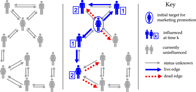
Figure 3: Illustration of the Adaptive Viral Marketing problem. Left: the underlying social network. Middle: the people influenced and the observations obtained after one person is selected.

8.1 Adaptive Viral Marketing

The viral marketing problem has a very natural adaptive analog. Instead of selecting a fixed set of people in advance, we may select a person to offer the promotion to, make some observations about the resulting spread of demand for our product, and repeat. See Fig. 3 for an illustration. In §8.2, we use the idea of adaptive submodularity to obtain results analogous to those of Kempe et al. (2003) in the adaptive setting. Specifically, we show that the greedy policy obtains at least $\left({1-\frac{1}{e}}\right)$ of the value of the best policy. Moreover, we extend this result by achieving that guarantee not only for the case where our reward is simply the number of influenced people, but also for any (nonnegative) monotone submodular function of the set of people influenced. In §8.3 we consider the minimum cost cover objective, and show that the greedy policy obtains a squared logarithmic approximation for it. To our knowledge, no approximation results for this adaptive variant of the viral marketing problem have been known.

8.1.1 Independent Cascade Model

In this model, the social network is a directed graph $G=(V,A)$ where each vertex in $V$ is a person, and each edge $(u,v)\in A$ has an associated binary random variable $X_{uv}$ indicating if $u$ will influence $v$. That is, $X_{uv}=1$ if $u$ will influence $v$ once it has been influenced, and $X_{uv}=0$ otherwise. The random variables $X_{uv}$ are independent, and have known means $p_{uv}:=\mathbb{E}\left[X_{uv}\right]$. We will call an edge $(u,v)$ with $X_{uv}=1$ a live edge and an edge with $X_{uv}=0$ a dead edge. When a node $u$ is activated, the edges $X_{uv}$ to each neighbor $v$ of $u$ are sampled, and $v$ is activated if $(u,v)$ is live. Influence can then spread from $u$’s neighbors to their neighbors, and so on, according to the same process. Once active, nodes remain active throughout the process, however Kempe et al. (2003) show that this assumption is without loss of generality, and can be removed.

8.1.2 The Feedback Model

In the Adaptive Viral Marketing problem under the independent cascades model, the items correspond to people we can activate by offering them the promotional deal. How we define the states ${\color[rgb]{0,0,0}{\phi}}(u)$ depends on what information we obtain as a result of activating $u$. Given the nature of the diffusion process, activating $u$ can have wide-ranging effects, so the state ${\color[rgb]{0,0,0}{\phi}}(u)$ has more to do with the state of the social network on the whole than with $u$ in particular. Specifically, we model ${\color[rgb]{0,0,0}{\phi}}(u)$ as a function ${\color[rgb]{0,0,0}{\phi}}_{u}:A\to\left\{0,1,?\right\}$, where ${\color[rgb]{0,0,0}{\phi}}_{u}((u,v))=0$ means that activating $u$ has revealed that $(u,v)$ is dead, ${\color[rgb]{0,0,0}{\phi}}_{u}((u,v))=1$ means that activating $u$ has revealed that $(u,v)$ is live, and ${\color[rgb]{0,0,0}{\phi}}_{u}((u,v))=\ ?$ means that activating $u$ has not revealed the status of $(u,v)$ (i.e., the value of $X_{uv}$). We require each realization to be consistent and complete. Consistency means that no edge should be declared both live and dead by any two states. That is, for all $u,v\in V$ and $a\in A$, $({\color[rgb]{0,0,0}{\phi}}_{u}(a),{\color[rgb]{0,0,0}{\phi}}_{v}(a))\notin\left\{(0,1),(1,0)\right\}$. Completeness means that the status of each edge is revealed by some activation. That is, for all $a\in A$ there exists $u\in V$ such that ${\color[rgb]{0,0,0}{\phi}}_{u}(a)\in\left\{0,1\right\}$. A consistent and complete realization thus encodes $X_{uv}$ for each edge $(u,v)$. Let ${A({{\color[rgb]{0,0,0}{\phi}}})}$ denote the live edges as encoded by ${\color[rgb]{0,0,0}{\phi}}$. There are several candidates for which edge sets we are allowed to observe when activating a node $u$. Here we consider what we call the Full-Adoption Feedback Model: After activating $u$ we get to see the status (live or dead) of all edges exiting $v$, for all nodes $v$ reachable from $u$ via live edges (i.e., reachable from $u$ in $(V,{A({{\color[rgb]{0,0,0}{\phi}}})})$, where ${\color[rgb]{0,0,0}{\phi}}$ is the true realization. We illustrate the full-adoption feedback model in Fig. 3.

8.1.3 The Objective Function

In the simplest case, the reward for influencing a set $U\subseteq V$ of nodes is $\hat{f}(U):=|U|$. Kempe et al. (2003) obtain an $\left({1-\frac{1}{e}}\right)$-approximation for the slightly more general case in which each node $u$ has a weight $w_{u}$ indicating its importance, and the reward is $\hat{f}(U):=\sum_{u\in U}w_{u}$. We generalize this result further, to include arbitrary nonnegative monotone submodular reward functions $\hat{f}$. This allows us, for example, to encode a value associated with the diversity of the set of nodes influenced, such as the notion that it is better to achieve $20\%$ market penetration in five different (equally important) demographic segments than $100\%$ market penetration in one and $0\%$ in the others.

8.2 Guarantees for the Maximum Coverage Objective

We are now ready to formally state our result for the maximum coverage objective.

Theorem 19

The greedy policy $\pi^{\text{greedy}}$ obtains at least $\left({1-\frac{1}{e}}\right)$ of the value of the best policy for the Adaptive Viral Marketing problem with arbitrary monotone submodular reward functions, in the independent cascade and full-adoption feedback models discussed above. That is, if $\sigma(S,{\color[rgb]{0,0,0}{\phi}})$ is the set of all activated nodes when $S$ is the seed set of activated nodes and ${\color[rgb]{0,0,0}{\phi}}$ is the realization, $\hat{f}:2^{V}\to\mathbb{R}_{\geq 0}$ is an arbitrary monotone submodular function indicating the reward for influencing a set, and the objective function is $f(S,{\color[rgb]{0,0,0}{\phi}}):=\hat{f}(\sigma(S,{\color[rgb]{0,0,0}{\phi}}))$, then for all policies $\pi$ and all $k\in\mathbb{N}$ we have

$$f_{\text{avg}}(\pi^{\text{greedy}}_{[{k}]})\geq\left({1-\frac{1}{e}}\right)f_{\text{avg}}(\pi_{[{k}]}).$$

More generally, if $\pi$ is an $\alpha$-approximate greedy policy then $\forall\ell\in\mathbb{N}$, $f_{\text{avg}}(\pi_{[{\ell}]})\geq\left({1-e^{-\ell/\alpha k}}\right)f_{\text{avg}}(\pi^{*}_{[{k}]})$.

Proof  Adaptive monotonicity follows immediately from the fact that $f(\cdot,{\color[rgb]{0,0,0}{\phi}})$ is monotonic for each ${\color[rgb]{0,0,0}{\phi}}$. It thus suffices to prove that $f$ is adaptive submodular with respect to the probability distribution on realizations ${\color[rgb]{0,0,0}{p\left({{\color[rgb]{0,0,0}{\phi}}}\right)}}$, because then we can invoke Theorem 5 to complete the proof.

We will say we have observed an edge $(u,v)$ if we know its status, i.e., if it is live or dead. Fix any ${\color[rgb]{0,0,0}{\psi}},{\color[rgb]{0,0,0}{\psi}}^{\prime}$ such that ${\color[rgb]{0,0,0}{\psi}}\subseteq{\color[rgb]{0,0,0}{\psi}}^{\prime}$ and any $v\notin\operatorname{dom}({\color[rgb]{0,0,0}{\psi}}^{\prime})$. We must show $\Delta\left({{v}\!\mid\!{{\color[rgb]{0,0,0}{\psi}}^{\prime}}}\right)\leq\Delta\left({{v}\!\mid\!{{\color[rgb]{0,0,0}{\psi}}}}\right)$. To prove this rigorously, we define a coupled distribution $\mu$ over pairs of realizations ${\color[rgb]{0,0,0}{\phi}}\sim{\color[rgb]{0,0,0}{\psi}}$ and ${\color[rgb]{0,0,0}{\phi}}^{\prime}\sim{\color[rgb]{0,0,0}{\psi}}^{\prime}$. Note that given the feedback model, the realization ${\color[rgb]{0,0,0}{\phi}}$ is a function of the random variables $\left\{X_{uw}:(u,w)\in A\right\}$ indicating the status of each edge. For conciseness we use the notation $\mathbf{X}=\left\{X_{uw}:(u,w)\in A\right\}$. We define $\mu$ implicitly in terms of a joint distribution $\hat{\mu}$ on $\mathbf{X}\times\mathbf{X}^{\prime}$, where ${\color[rgb]{0,0,0}{\phi}}={\color[rgb]{0,0,0}{\phi}}(\mathbf{X})$ and ${\color[rgb]{0,0,0}{\phi}}^{\prime}={\color[rgb]{0,0,0}{\phi}}^{\prime}(\mathbf{X}^{\prime})$ are the realizations induced by the two distinct sets of random edge statuses, respectively. Hence $\mu({\color[rgb]{0,0,0}{\phi}}(\mathbf{X}),{\color[rgb]{0,0,0}{\phi}}(\mathbf{X}^{\prime}))=\hat{\mu}(\mathbf{X},\mathbf{X}^{\prime})$. Next, let us say a partial realization ${\color[rgb]{0,0,0}{\psi}}$ observes an edge $e$ if some $w\in\operatorname{dom}({\color[rgb]{0,0,0}{\psi}})$ has revealed its status as being live or dead. For edges $(u,w)$ observed by ${\color[rgb]{0,0,0}{\psi}}$, the random variable $X_{uw}$ is deterministically set to the status observed by ${\color[rgb]{0,0,0}{\psi}}$. Similarly, for edges $(u,w)$ observed by ${\color[rgb]{0,0,0}{\psi}}^{\prime}$, the random variable $X^{\prime}_{uw}$ is deterministically set to the status observed by ${\color[rgb]{0,0,0}{\psi}}^{\prime}$. Note that since ${\color[rgb]{0,0,0}{\psi}}\subseteq{\color[rgb]{0,0,0}{\psi}}^{\prime}$, the state of all edges which are observed by ${\color[rgb]{0,0,0}{\psi}}$ are the same in ${\color[rgb]{0,0,0}{\phi}}$ and ${\color[rgb]{0,0,0}{\phi}}^{\prime}$. All $(\mathbf{X},\mathbf{X}^{\prime})\in\operatorname{support}(\hat{\mu})$ have these properties. Additionally, we will construct $\hat{\mu}$ so that the status of all edges which are unobserved by both ${\color[rgb]{0,0,0}{\psi}}^{\prime}$ and ${\color[rgb]{0,0,0}{\psi}}$ are the same in $\mathbf{X}$ and $\mathbf{X}^{\prime}$, meaning $X_{uw}=X^{\prime}_{uw}$ for all such edges $(u,w)$, or else $\hat{\mu}(\mathbf{X},\mathbf{X}^{\prime})=0$.

The above constraints leave us with the following degrees of freedom: we may select $X_{uw}$ for all $(u,w)\in A$ which are unobserved by ${\color[rgb]{0,0,0}{\psi}}$. We select them independently, such that $\mathbb{E}\left[X_{uw}\right]=p_{uw}$ as with the prior ${\color[rgb]{0,0,0}{p\left({{\color[rgb]{0,0,0}{\phi}}}\right)}}$. Hence for all $(\mathbf{X},\mathbf{X}^{\prime})$ satisfying the above constraints,

$$\hat{\mu}(\mathbf{X},\mathbf{X}^{\prime})=\prod_{(u,w)\text{ unobserved by }{\color[rgb]{0,0,0}{\psi}}}p_{uw}^{X_{uw}}\left({1-p_{uw}}\right)^{1-X_{uw}},$$

and otherwise $\hat{\mu}(\mathbf{X},\mathbf{X}^{\prime})=0$. Note that ${\color[rgb]{0,0,0}{p\left({{\color[rgb]{0,0,0}{\phi}}\mid{\color[rgb]{0,0,0}{\psi}}}\right)}}=\sum_{{\color[rgb]{0,0,0}{\phi}}^{\prime}}\mu({\color[rgb]{0,0,0}{\phi}},{\color[rgb]{0,0,0}{\phi}}^{\prime})$ and ${\color[rgb]{0,0,0}{p\left({{\color[rgb]{0,0,0}{\phi}}^{\prime}\mid{\color[rgb]{0,0,0}{\psi}}^{\prime}}\right)}}=\sum_{{\color[rgb]{0,0,0}{\phi}}}\mu({\color[rgb]{0,0,0}{\phi}},{\color[rgb]{0,0,0}{\phi}}^{\prime})$. We next claim that for all $({\color[rgb]{0,0,0}{\phi}},{\color[rgb]{0,0,0}{\phi}}^{\prime})\in\operatorname{support}(\mu)$

$$f(\operatorname{dom}({\color[rgb]{0,0,0}{\psi}}^{\prime})\cup\left\{v\right\},{\color[rgb]{0,0,0}{\phi}}^{\prime})-f(\operatorname{dom}({\color[rgb]{0,0,0}{\psi}}^{\prime}),{\color[rgb]{0,0,0}{\phi}}^{\prime}) \leq f(\operatorname{dom}({\color[rgb]{0,0,0}{\psi}})\cup\left\{v\right\},{\color[rgb]{0,0,0}{\phi}})-f(\operatorname{dom}({\color[rgb]{0,0,0}{\psi}}),{\color[rgb]{0,0,0}{\phi}}).\quad$$ (19)

Recall $f(S,{\color[rgb]{0,0,0}{\phi}}):=\hat{f}(\sigma(S,{\color[rgb]{0,0,0}{\phi}}))$, where $\sigma(S,{\color[rgb]{0,0,0}{\phi}})$ is the set of all activated nodes when $S$ is the seed set of activated nodes and ${\color[rgb]{0,0,0}{\phi}}$ is the realization. Let $B=\sigma(\operatorname{dom}({\color[rgb]{0,0,0}{\psi}}),{\color[rgb]{0,0,0}{\phi}})$ and $C=\sigma(\operatorname{dom}({\color[rgb]{0,0,0}{\psi}})\cup\left\{v\right\},{\color[rgb]{0,0,0}{\phi}})$ denote the active nodes before and after selecting $v$ after $\operatorname{dom}({\color[rgb]{0,0,0}{\psi}})$ under realizations ${\color[rgb]{0,0,0}{\phi}}$, and similarly define $B^{\prime}$ and $C^{\prime}$ with respect to ${\color[rgb]{0,0,0}{\psi}}^{\prime}$ and ${\color[rgb]{0,0,0}{\phi}}^{\prime}$. Let $D:=C\setminus B$, $D^{\prime}:=C^{\prime}\setminus B^{\prime}$. Then Eq. (19) is equivalent to $\hat{f}(B^{\prime}\cup D^{\prime})-\hat{f}(B^{\prime})\leq\hat{f}(B\cup D)-\hat{f}(B)$. By the submodularity of $\hat{f}$, it suffices to show that $B\subseteq B^{\prime}$ and $D^{\prime}\subseteq D$ to prove the above inequality, which we will now do.

We start by proving $B\subseteq B^{\prime}$. Fix $w\in B$. Then there exists a path from some $u\in\operatorname{dom}({\color[rgb]{0,0,0}{\psi}})$ to $w$ in $(V,{A({{\color[rgb]{0,0,0}{\phi}}})})$. Moreover, every edge in this path is not only live but also observed to be live, by definition of the feedback model. Since $({\color[rgb]{0,0,0}{\phi}},{\color[rgb]{0,0,0}{\phi}}^{\prime})\in\operatorname{support}(\mu)$, this implies that every edge in this path is also live under ${\color[rgb]{0,0,0}{\phi}}^{\prime}$, as edges observed by ${\color[rgb]{0,0,0}{\psi}}$ must have the same status under both ${\color[rgb]{0,0,0}{\phi}}$ and ${\color[rgb]{0,0,0}{\phi}}^{\prime}$. It follows that there is a path from $u$ to $w$ in $(V,{A({{\color[rgb]{0,0,0}{\phi}}^{\prime}})})$. Since $u$ is clearly also in $\operatorname{dom}({\color[rgb]{0,0,0}{\psi}}^{\prime})$, we conclude $w\in B^{\prime}$, hence $B\subseteq B^{\prime}$.

Next we show $D^{\prime}\subseteq D$. Fix some $w\in D^{\prime}$ and suppose by way of contradiction that $w\notin D$. Hence there exists a path $P$ from $v$ to $w$ in $(V,{A({{\color[rgb]{0,0,0}{\phi}}^{\prime}})})$ but no such path exists in $(V,{A({{\color[rgb]{0,0,0}{\phi}}})})$. The edges of $P$ are all live under ${\color[rgb]{0,0,0}{\phi}}^{\prime}$, and at least one must be dead under ${\color[rgb]{0,0,0}{\phi}}$. Let $(u,u^{\prime})$ be such an edge in $P$. Because the status of this edge differs in ${\color[rgb]{0,0,0}{\phi}}$ and ${\color[rgb]{0,0,0}{\phi}}^{\prime}$, and $({\color[rgb]{0,0,0}{\phi}},{\color[rgb]{0,0,0}{\phi}}^{\prime})\in\operatorname{support}(\mu)$, it must be that $(u,u^{\prime})$ is observed by ${\color[rgb]{0,0,0}{\psi}}^{\prime}$ but not observed by ${\color[rgb]{0,0,0}{\psi}}$. Because it is observed by ${\color[rgb]{0,0,0}{\psi}}^{\prime}$, in our feedback model it must be that $u$ is active after $\operatorname{dom}({\color[rgb]{0,0,0}{\psi}}^{\prime})$ is selected, i.e., $u\in B^{\prime}$. However, this implies that all nodes reachable from $u$ via edges in $P$ are also active after $\operatorname{dom}({\color[rgb]{0,0,0}{\psi}}^{\prime})$ is selected, since all the edges in $P$ are live. Hence all such nodes, including $w$, are in $B^{\prime}$. Since $D^{\prime}$ and $B^{\prime}$ are disjoint, this implies $w\notin D^{\prime}$, a contradiction.

Having proved Eq. (19), we now proceed to use it to show $\Delta\left({{v}\!\mid\!{{\color[rgb]{0,0,0}{\psi}}^{\prime}}}\right)\leq\Delta\left({{v}\!\mid\!{{\color[rgb]{0,0,0}{\psi}}}}\right)$ as in §6.

$$\begin{array}[]{lllll}\Delta\left({{v}\!\mid\!{{\color[rgb]{0,0,0}{\psi}}^{\prime}}}\right)&=&\sum_{({\color[rgb]{0,0,0}{\phi}},{\color[rgb]{0,0,0}{\phi}}^{\prime})}\mu({\color[rgb]{0,0,0}{\phi}},{\color[rgb]{0,0,0}{\phi}}^{\prime})\left({f(\operatorname{dom}({\color[rgb]{0,0,0}{\psi}}^{\prime})\cup\left\{v\right\},{\color[rgb]{0,0,0}{\phi}}^{\prime})-f(\operatorname{dom}({\color[rgb]{0,0,0}{\psi}}^{\prime}),{\color[rgb]{0,0,0}{\phi}}^{\prime})}\right)&&\\[8.53581pt] &\leq&\sum_{({\color[rgb]{0,0,0}{\phi}},{\color[rgb]{0,0,0}{\phi}}^{\prime})}\mu({\color[rgb]{0,0,0}{\phi}},{\color[rgb]{0,0,0}{\phi}}^{\prime})\left({f(\operatorname{dom}({\color[rgb]{0,0,0}{\psi}})\cup\left\{v\right\},{\color[rgb]{0,0,0}{\phi}})-f(\operatorname{dom}({\color[rgb]{0,0,0}{\psi}}),{\color[rgb]{0,0,0}{\phi}})}\right)&=&\Delta\left({{v}\!\mid\!{{\color[rgb]{0,0,0}{\psi}}}}\right)\end{array}$$

which completes the proof.  

8.2.1 Comparison with Stochastic Submodular Maximization

It is worth contrasting the Adaptive Viral Marketing problem with the Stochastic Submodular Maximization problem of §6. In the latter problem, we can think of the items as being random independently distributed sets. In Adaptive Viral Marketing by contrast, the random sets (of nodes influenced when a fixed node is selected) depend on the random status of the edges, and hence may be correlated through them. Nevertheless, we can obtain the same $\left({1-\frac{1}{e}}\right)$ approximation factor for both problems.

A Comment on the Myopic Feedback Model.

In the conference version of this article (Golovin and Krause, 2010), we considered an alternate feedback model called the myopic feedback model, in which after activating $v$ we see the status of all edges exiting $v$ in the social network, i.e., $\partial_{+}(u):=\left\{(u,v):v\in V\right\}\cap A$. We claimed that the objective $f$ as defined previously is adaptive submodular in the independent cascade model with myopic feedback, and hence the greedy policy obtains a $(1-\frac{1}{e})$ approximation for it. We hereby retract this claim, and furthermore give a counterexample demonstrating that $f$ is not adaptive submodular under myopic feedback.

Consider a graph $G=(V,E)$ with vertices $V:=\left\{u,v,w\right\}$, and edges $E:=\left\{(u,v),(v,w)\right\}$. The edge parameters are $p_{uv}=1$ and $p_{vw}=1-\epsilon$. Let $\hat{f}(U)=|U|$ and construct $f$ from $\hat{f}$ accordingly. We let ${\color[rgb]{0,0,0}{\psi}}=\left\{(u,{\color[rgb]{0,0,0}{\phi}}_{u})\right\}$, where ${\color[rgb]{0,0,0}{\phi}}_{u}((u,v))=1$ and ${\color[rgb]{0,0,0}{\phi}}_{u}((v,w))=\ ?$. Let ${\color[rgb]{0,0,0}{\psi}}^{\prime}=\left\{(u,{\color[rgb]{0,0,0}{\phi}}_{u}),(v,{\color[rgb]{0,0,0}{\phi}}_{v})\right\}$ where ${\color[rgb]{0,0,0}{\phi}}_{v}((v,w))=0$. Clearly, ${\color[rgb]{0,0,0}{\psi}}\subset{\color[rgb]{0,0,0}{\psi}}^{\prime}$. Note $\Delta\left({{w}\!\mid\!{{\color[rgb]{0,0,0}{\psi}}}}\right)=\epsilon$, since the marginal benefit of $w$ over $\operatorname{dom}({\color[rgb]{0,0,0}{\psi}})$ is one if $(v,w)$ is dead, and zero if it is live, and the former occurs with probability $\epsilon$. In contrast, $\Delta\left({{w}\!\mid\!{{\color[rgb]{0,0,0}{\psi}}^{\prime}}}\right)=1$, since ${\color[rgb]{0,0,0}{\psi}}^{\prime}$ contains the observation that $(v,w)$ is dead. Hence $\Delta\left({{w}\!\mid\!{{\color[rgb]{0,0,0}{\psi}}}}\right)<\Delta\left({{w}\!\mid\!{{\color[rgb]{0,0,0}{\psi}}^{\prime}}}\right)$, which violates adaptive submodularity. However, we conjecture that the greedy policy still obtains a constant factor approximation even in the myopic feedback model.

8.3 The Minimum Cost Cover Objective

We may also wish to adaptively run our campaign until a certain level of market penetration has been achieved, e.g., a certain number of people have adopted the product. We can formalize this goal using the minimum cost cover objective. For this objective, we have an instance of Adaptive Stochastic Minimum Cost Cover, in which we are given a quota $Q\leq\hat{f}(V)$ (quantifying the desired level of market penetration) and we must adaptively select nodes to activate until the set of all active nodes $S$ satisfies $\hat{f}(S)\geq Q$. We obtain the following result.

Theorem 20

Fix a monotone submodular function $\hat{f}:2^{V}\to\mathbb{R}_{\geq 0}$ indicating the reward for influencing a set, and a quota $Q\leq\hat{f}(V)$. Suppose the objective is $f(S,{\color[rgb]{0,0,0}{\phi}}):=\min\left\{Q,\hat{f}(\sigma(S,{\color[rgb]{0,0,0}{\phi}}))\right\}$, where $\sigma(S,{\color[rgb]{0,0,0}{\phi}})$ is the set of all activated nodes when $S$ is the seed set of activated nodes and ${\color[rgb]{0,0,0}{\phi}}$ is the realization. Let $\eta$ be any value such that $\hat{f}(S)>Q-\eta$ implies $\hat{f}(S)\geq Q$ for all $S$. Then any $\alpha$-approximate greedy policy $\pi$ on average costs at most $\alpha\left({\ln\left({\frac{Q}{\eta}}\right)+1}\right)^{2}$ times the average cost of the best policy obtaining $Q$ reward for the Adaptive Viral Marketing problem in the independent cascade model with full-adoption feedback as described above. That is, ${c_{\text{avg}}{(\pi)}}\leq\alpha\left({\ln\left({\frac{Q}{\eta}}\right)+1}\right)^{2}{c_{\text{avg}}{(\pi^{*})}}$ for any $\pi^{*}$ that covers every realization.

Proof  We prove Theorem 20 by recourse to Theorem 13. We have already established that $f$ is adaptive submodular, in the proof of Theorem 19. It remains to show that $f$ is strongly adaptive monotone and strongly adaptive submodular, that these instances are self–certifying, and that $Q$ and $\eta$ equal the corresponding terms in the statement of Theorem 13.

We start with strong adaptive monotonicity. Fix ${\color[rgb]{0,0,0}{\psi}}$, $e\notin\operatorname{dom}({\color[rgb]{0,0,0}{\psi}})$, and $o\in O$. We must show

$$\mathbb{E}\left[f(\operatorname{dom}({\color[rgb]{0,0,0}{\psi}}),{\color[rgb]{0,0,0}{\Phi}})\ \mid\ {\color[rgb]{0,0,0}{\Phi}}\sim{\color[rgb]{0,0,0}{\psi}}\right]\leq\mathbb{E}\left[f(\operatorname{dom}({\color[rgb]{0,0,0}{\psi}})\cup\left\{e\right\},{\color[rgb]{0,0,0}{\Phi}})\ \mid\ {\color[rgb]{0,0,0}{\Phi}}\sim{\color[rgb]{0,0,0}{\psi}},{\color[rgb]{0,0,0}{\Phi}}(e)=o\right].$$ (20)

Let $V^{+}\!\left({{\color[rgb]{0,0,0}{\psi}}}\right)$ denote the active nodes after selecting $\operatorname{dom}({\color[rgb]{0,0,0}{\psi}})$ and observing ${\color[rgb]{0,0,0}{\psi}}$. By definition of the full adoption feedback model, $V^{+}\!\left({{\color[rgb]{0,0,0}{\psi}}}\right)$ consists of precisely those nodes $v$ for which there exists a path $P_{uv}$ from some $u\in\operatorname{dom}({\color[rgb]{0,0,0}{\psi}})$ to $v$ via exclusively live edges. The edges whose status we observe consist of all edges exiting nodes in $V^{+}\!\left({{\color[rgb]{0,0,0}{\psi}}}\right)$. It follows that every path from any $u\in V^{+}\!\left({{\color[rgb]{0,0,0}{\psi}}}\right)$ to any $v\in V\setminus V^{+}\!\left({{\color[rgb]{0,0,0}{\psi}}}\right)$ contains at least one edge which is observed by ${\color[rgb]{0,0,0}{\psi}}$ to be dead. Hence, in every ${\color[rgb]{0,0,0}{\phi}}\sim{\color[rgb]{0,0,0}{\psi}}$, the set of nodes activated by selecting $\operatorname{dom}({\color[rgb]{0,0,0}{\psi}})$ is the same. Therefore $\mathbb{E}\left[f(\operatorname{dom}({\color[rgb]{0,0,0}{\psi}}),{\color[rgb]{0,0,0}{\Phi}})\ \mid\ {\color[rgb]{0,0,0}{\Phi}}\sim{\color[rgb]{0,0,0}{\psi}}\right]=\hat{f}(V^{+}\!\left({{\color[rgb]{0,0,0}{\psi}}}\right))$. Similarly, if we define ${\color[rgb]{0,0,0}{\psi}}^{\prime}:={\color[rgb]{0,0,0}{\psi}}\cup\left\{(e,o)\right\}$, then $\mathbb{E}\left[f(\operatorname{dom}({\color[rgb]{0,0,0}{\psi}})\cup\left\{e\right\},{\color[rgb]{0,0,0}{\Phi}})\ \mid\ {\color[rgb]{0,0,0}{\Phi}}\sim{\color[rgb]{0,0,0}{\psi}},{\color[rgb]{0,0,0}{\Phi}}(e)=o\right]=\hat{f}(V^{+}\!\left({{\color[rgb]{0,0,0}{\psi}}^{\prime}}\right))$. Note that once activated, nodes never become inactive. Hence, ${\color[rgb]{0,0,0}{\psi}}\subseteq{\color[rgb]{0,0,0}{\psi}}^{\prime}$ implies $V^{+}\!\left({{\color[rgb]{0,0,0}{\psi}}}\right)\subseteq V^{+}\!\left({{\color[rgb]{0,0,0}{\psi}}^{\prime}}\right)$. Since $\hat{f}$ is monotone by assumption, this means $\hat{f}(V^{+}\!\left({{\color[rgb]{0,0,0}{\psi}}}\right))\leq\hat{f}(V^{+}\!\left({{\color[rgb]{0,0,0}{\psi}}^{\prime}}\right))$ which implies Eq. (20) and strong adaptive monotonicity.

Next we establish strong adaptive submodularity. Given that we have already established adaptive submodularity, it is sufficient to also prove pointwise submodularity. For a fixed realization ${\color[rgb]{0,0,0}{\phi}}$ we have a set of live edges $\left\{(u,v):X_{uv}=1\right\}$ which induce a set system in which $u$ covers all nodes reachable from $u$ via live edges. Let $S_{u}$ denote this set. It is straightforward to verify that a monotone submodular function $\hat{f}$ on nodes induces a monotone submodular function on sets of those nodes. That is,

$$g(A):=\hat{f}\left({\cup_{u\in A}S_{u}}\right)$$

is submodular whenever $\hat{f}$ is. In particular, $g$ is submodular if for every $A$ and $B$ we have $g(A)+g(B)\geq g(A\cap B)+g(A\cup B)$ however one can easily verify that this set of constraints is a subset of the corresponding submodularity constaints on $\hat{f}$.

Next we establish that these instances are self–certifying. Note that for every ${\color[rgb]{0,0,0}{\phi}}$ we have $f(V,{\color[rgb]{0,0,0}{\phi}})=\min\left\{Q,\hat{f}(V)\right\}=Q$. From our earlier remarks, we know that $f(\operatorname{dom}({\color[rgb]{0,0,0}{\psi}}),{\color[rgb]{0,0,0}{\phi}})=\hat{f}(V^{+}\!\left({{\color[rgb]{0,0,0}{\psi}}}\right))$ for every ${\color[rgb]{0,0,0}{\phi}}\sim{\color[rgb]{0,0,0}{\psi}}$. Hence for all ${\color[rgb]{0,0,0}{\psi}}$ and ${\color[rgb]{0,0,0}{\phi}},{\color[rgb]{0,0,0}{\phi}}^{\prime}$ consistent with ${\color[rgb]{0,0,0}{\psi}}$, we have $f(\operatorname{dom}({\color[rgb]{0,0,0}{\psi}}),{\color[rgb]{0,0,0}{\phi}})=f(\operatorname{dom}({\color[rgb]{0,0,0}{\psi}}),{\color[rgb]{0,0,0}{\phi}}^{\prime})$ and so $f(\operatorname{dom}({\color[rgb]{0,0,0}{\psi}}),{\color[rgb]{0,0,0}{\phi}})=Q$ if and only if $f(\operatorname{dom}({\color[rgb]{0,0,0}{\psi}}),{\color[rgb]{0,0,0}{\phi}}^{\prime})=Q$, which proves that the instance is self–certifying.

Finally we show that $Q$ and $\eta$ equal the corresponding terms in the statement of Theorem 13. As noted earlier, $f(V,{\color[rgb]{0,0,0}{\phi}})=Q$ for all ${\color[rgb]{0,0,0}{\phi}}$. We defined $\eta$ as some value such that $\hat{f}(S)>Q-\eta$ implies $\hat{f}(S)\geq Q$ for all $S$. Since $\operatorname{range}(f)=\left\{\min\left\{Q,\hat{f}(S)\right\}:S\subseteq V\right\}$, it follows that we cannot have $f(S,{\color[rgb]{0,0,0}{\phi}})\in(Q-\eta,Q)$ for any $S$ and ${\color[rgb]{0,0,0}{\phi}}$, so that $\eta$ satisfies the requirements of the corresponding term in Theorem 13. Hence we may apply Theorem 13 on this self–certifying instance with $Q$ and $\eta$ to obtain the claimed result.  

9 Application: Automated Diagnosis and Active Learning

An important problem in AI is automated diagnosis. For example, suppose we have different hypotheses about the state of a patient, and can run medical tests to rule out inconsistent hypotheses. The goal is to adaptively choose tests to infer the state of the patient as quickly as possible.

A similar problem arises in active learning. Obtaining labeled data to train a classifier is typically expensive, as it often involves asking an expert. In active learning (c.f. Cohn et al. (1996); McCallum and Nigam (1998)), the key idea is that some labels are more informative than others: labeling a few unlabeled examples can imply the labels of many other unlabeled examples, and thus the cost of obtaining the labels from an expert can be avoided. As is standard, we assume that we are given a set of hypotheses $H$, and a set of unlabeled data points $X$ where each $x\in X$ is independently drawn from some distribution $\mathcal{D}$. Let $L$ be the set of possible labels. Classical learning theory yields probably approximately correct (PAC) bounds, bounding the number $n$ of examples drawn i.i.d. from $\mathcal{D}$ needed to output a hypothesis $h$ that will have expected error at most $\varepsilon$ with probability at least $1-\delta$, for some fixed $\varepsilon,\delta>0$. That is, if $h^{*}$ is the target hypothesis (with zero error), and $\operatorname{error}(h):=\mathbb{P}_{x\sim\mathcal{D}}\left[h(x)\neq h^{*}(x)\right]$ is the error of $h$, we require $\mathbb{P}\left[\operatorname{error}(h)\leq\varepsilon\right]\geq 1-\delta$. The latter probability is taken with respect to $\mathcal{D}(X)$; the learned hypothesis $h$ and thus $\operatorname{error}(h)$ depend on it. A key challenge in active learning is to avoid bias: actively selected examples are no longer i.i.d., and thus sample complexity bounds for passive learning no longer apply. If one is not careful, active learning may require more samples than passive learning to achieve the same generalization error. One natural approach to active learning that is guaranteed to perform at least as well as passive learning is pool-based active learning (McCallum and Nigam, 1998): The idea is to draw $n$ unlabeled examples i.i.d. However, instead of obtaining all labels, labels are adaptively requested until the labels of all unlabeled examples are implied by the obtained labels. Now we have obtained $n$ labeled examples drawn i.i.d., and classical PAC bounds still apply. The key question is how to request the labels for the pool to infer the remaining labels as quickly as possible.

In the case of binary labels (or test outcomes) $L=\left\{-1,1\right\}$, various authors have considered greedy policies which generalize binary search (Garey and Graham, 1974; Loveland, 1985; Arkin et al., 1993; Kosaraju et al., 1999; Dasgupta, 2004; Guillory and Bilmes, 2009; Nowak, 2009). The simplest of these, called generalized binary search (GBS) or the splitting algorithm, works as follows. Define the version space $V$ to be the set of hypotheses consistent with the observed labels (here we assume that there is no label noise). In the worst-case setting, GBS selects a query $x\in X$ that minimizes $\left|\sum_{h\in V}h(x)\right|$. In the Bayesian setting we assume we are given a prior $p_{H}$ over hypotheses; in this case GBS selects a query $x\in X$ that minimizes $\left|\sum_{h\in V}p_{H}(h)\cdot h(x)\right|$. Intuitively these policies myopically attempt to shrink a measure of the version space (i.e., the cardinality or the probability mass) as quickly as possible. The former provides an ${\mathcal{O}}(\log|H|)$-approximation for the worst-case number of queries (Arkin et al., 1993), and the latter provides an ${\mathcal{O}}(\log\frac{1}{\min_{h}p_{H}(h)})$-approximation for the expected number of queries (Kosaraju et al., 1999; Dasgupta, 2004) and a natural generalization of GBS obtains the same guarantees with a larger set of labels (Guillory and Bilmes, 2009). Kosaraju et al. also prove that running GBS on a modified prior $p_{H}^{\prime}(h)\propto\max\left\{p_{H}(h),1/|H|^{2}\log|H|\right\}$ is sufficient to obtain an ${\mathcal{O}}(\log|H|)$-approximation.

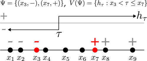
Figure 4: Illustration of the Active Learning problem, in the simple special case of one-dimensional data and binary threshold hypotheses $H=\left\{h_{\tau}:\tau\in\mathbb{R}\right\}$, where $h_{\tau}(x)=1$ if $x\geq\tau$ and $0$ otherwise.

Viewed from this perspective of the previous sections, shrinking the version space amounts to “covering” all false hypotheses with stochastic sets (i.e., queries), where query $x$ covers all hypotheses that disagree with the target hypothesis $h^{*}$ at $x$. That is, $x$ covers $\left\{h:h(x)\neq h^{*}(x)\right\}$. As in §8, these sets may be correlated in complex ways determined by the set of possible hypotheses. As we will show, the reduction in version space mass is adaptive submodular, and this allows us to obtain a new analysis of GBS using adaptive submodularity, which has a weaker approximation guarantee than is optimal, but is arguably more amenable to extensions and generalizations than previous analyses.

Theorem 21

In the Bayesian setting in which there is a prior $p_{H}$ on a finite set of hypotheses $H$, the generalized binary search algorithm makes $\textsf{OPT}\cdot\left({\ln\left({\frac{1}{\min_{h}p_{H}(h)}}\right)+1}\right)^{2}$ queries in expectation to identify a hypothesis drawn from $p_{H}$, where OPT is the minimum expected number of queries made by any policy. If $\min_{h}p_{H}(h)$ is sufficiently small, running the algorithm on a modified prior $p_{H}^{\prime}(h)\propto\max\left\{p_{H}(h),1/|H|^{2}\right\}$ improves the approximation factor to ${\mathcal{O}}\left({\left({\ln|H|}\right)^{2}}\right)$.

We devote the better part of the remainder of this section to the proof of Theorem 21, which has several components. We first address the important special case of a uniform prior over hypotheses, i.e., $p_{H}(h)=1/|H|$ for all $h\in H$, and then we reduce the case with a general prior to a uniform prior. We wish to appeal to Theorem 13, so we convert the problem into an Adaptive Stochastic Min Cost Cover problem.

9.1 The Reduction to Adaptive Stochastic Min Cost Cover

Define a realization ${\color[rgb]{0,0,0}{\phi}}_{h}$ for each hypothesis $h\in H$. The ground set is $E=X$, and the outcomes are binary; we define $O=\left\{-1,1\right\}$ instead of using $\left\{0,1\right\}$ to be consistent with our earlier exposition. For all $h\in H$ we set ${\color[rgb]{0,0,0}{\phi}}_{h}\equiv h$, meaning ${\color[rgb]{0,0,0}{\phi}}_{h}(x)=h(x)$ for all $x\in X$. To define the objective function, we first need some notation. Given observed labels ${\color[rgb]{0,0,0}{\psi}}\subset X\times O$, let $V({\color[rgb]{0,0,0}{\psi}})$ denote the version space, i.e., the set of hypotheses for which $h(x)={\color[rgb]{0,0,0}{\psi}}(x)$ for all $x\in\operatorname{dom}({\color[rgb]{0,0,0}{\psi}})$. See Fig. 4 for an illustration of an active learning problem in the case of indicator hypotheses. For a set of hypotheses $V$, let $p_{H}(V):=\sum_{h\in V}p_{H}(h)$ denote their total prior probability. Finally, let ${\color[rgb]{0,0,0}{\psi}}(S,h)=\left\{(x,h(x))\ :\ x\in S\right\}$ be the function with domain $S$ that agrees with $h$ on $S$. We define the objective function by

$$f(S,{\color[rgb]{0,0,0}{\phi}}_{h})\ :=\ 1-p_{H}(V({\color[rgb]{0,0,0}{\psi}}(S,h)))\ =\ p_{H}\!\left({\left\{h^{\prime}\ :\ \exists x\in S,h^{\prime}(x)\neq h(x)\right\}}\right)$$

and use ${\color[rgb]{0,0,0}{p\left({{\color[rgb]{0,0,0}{\phi}}_{h}}\right)}}=p_{H}(h)=1/|H|$ for all $h$. Let $\pi^{*}$ be an optimal policy for this Adaptive Stochastic Min Cost Cover instance. Note that there is an exact correspondence between policies for the original problem of finding the target hypothesis and our problem of covering the true realization; $h^{*}$ is identified as the target hypothesis if and only if the version space is reduced to $\left\{h^{*}\right\}$ which occurs if and only if ${\color[rgb]{0,0,0}{\phi}}_{h^{*}}$ is covered. Hence ${c_{\text{avg}}{(\pi^{*})}}=\textsf{OPT}$. Note that because we have assumed a uniform prior over hypotheses, we have $f(X,{\color[rgb]{0,0,0}{\phi}}_{h})=1-1/|H|$ for all $h$. Furthermore, the instances are self–certifying.

Lemma 22

The instances described above are self–certifying for arbitrary priors $p_{H}$.

Proof  Intuitively, theses instances are self–certifying because to cover ${\color[rgb]{0,0,0}{\phi}}_{h^{*}}$ a policy must identify ${\color[rgb]{0,0,0}{\phi}}_{h^{*}}$. More formally, these instances are self–certifying because for any ${\color[rgb]{0,0,0}{\phi}}_{h}$ and ${\color[rgb]{0,0,0}{\psi}}$ such that ${\color[rgb]{0,0,0}{\phi}}_{h}\sim{\color[rgb]{0,0,0}{\psi}}$, we have that $f(\operatorname{dom}({\color[rgb]{0,0,0}{\psi}}),{\color[rgb]{0,0,0}{\phi}}_{h})=f(X,{\color[rgb]{0,0,0}{\phi}}_{h})$ implies $V({\color[rgb]{0,0,0}{\psi}})=\left\{h\right\}$. This in turn means that ${\color[rgb]{0,0,0}{\phi}}_{h}$ is the only realization consistent with ${\color[rgb]{0,0,0}{\psi}}$, which trivially implies that any realization ${\color[rgb]{0,0,0}{\phi}}^{\prime}\sim{\color[rgb]{0,0,0}{\psi}}$ also has $f(\operatorname{dom}({\color[rgb]{0,0,0}{\psi}}),{\color[rgb]{0,0,0}{\phi}}^{\prime})=f(X,{\color[rgb]{0,0,0}{\phi}}^{\prime})$; hence the instance is self–certifying.  

9.2 The Uniform Prior

We next prove that the instances generated are adaptive submodular and strongly adaptive monotone under a uniform prior.

Lemma 23

In the instances described above, $f$ is strongly adaptive monotone and strongly adaptive submodular and with respect to a uniform prior $p_{H}$.

Proof  Demonstrating strong adaptive monotonicity under a uniform prior amounts to proving that adding labels cannot grow the version space, which is clear in our model. That is, each query $x$ eliminates some subset of hypotheses, and as more queries are performed, the subset of hypotheses eliminated by $x$ cannot grow. Moving on to adaptive submodularity, consider the expected marginal contribution of $x$ under two partial realizations ${\color[rgb]{0,0,0}{\psi}},{\color[rgb]{0,0,0}{\psi}}^{\prime}$ where ${\color[rgb]{0,0,0}{\psi}}$ is a subrealization of ${\color[rgb]{0,0,0}{\psi}}^{\prime}$ (i.e., ${\color[rgb]{0,0,0}{\psi}}\subset{\color[rgb]{0,0,0}{\psi}}^{\prime}$), and $x\notin\operatorname{dom}({\color[rgb]{0,0,0}{\psi}}^{\prime})$. Let ${{\color[rgb]{0,0,0}{\psi}}}\!\left[{x}/{o}\right]$ be the partial realization with domain $\operatorname{dom}({\color[rgb]{0,0,0}{\psi}})\cup\left\{x\right\}$ that agrees with ${\color[rgb]{0,0,0}{\psi}}$ on its domain, and maps $x$ to $o$. For each $o\in O$, let $a_{o}:=p_{H}(V({{\color[rgb]{0,0,0}{\psi}}}\!\left[{x}/{o}\right]))$, $b_{o}:=p_{H}(V({{\color[rgb]{0,0,0}{\psi}}^{\prime}}\!\left[{x}/{o}\right]))$. Since a hypothesis eliminated from the version space cannot later appear in the version space, we have $a_{o}\geq b_{o}$ for all $o$. Next, note the expected reduction in version space mass (and hence the expected marginal contribution) due to selecting $x$ given partial realization ${\color[rgb]{0,0,0}{\psi}}$ is

$$\Delta\left({{x}\!\mid\!{{\color[rgb]{0,0,0}{\psi}}}}\right)=\sum_{o\in O}a_{o}\cdot\mathbb{P}\left[{\color[rgb]{0,0,0}{\Phi}}(x)\neq o\ \mid\ {\color[rgb]{0,0,0}{\Phi}}\sim{\color[rgb]{0,0,0}{\psi}}\right]=\sum_{o}a_{o}\left({\frac{\sum_{o^{\prime}\neq o}a_{o^{\prime}}}{\sum_{o^{\prime}}a_{o^{\prime}}}}\right)=\frac{\sum_{o\neq o^{\prime}}a_{o}a_{o^{\prime}}}{\sum_{o^{\prime}}a_{o^{\prime}}}.$$ (21)

The corresponding quantity for ${\color[rgb]{0,0,0}{\psi}}^{\prime}$ has $b_{o}$ substituted for $a_{o}$ in Eq. (21), for each $o\in O$. To prove adaptive submodularity we must show $\Delta\left({{x}\!\mid\!{{\color[rgb]{0,0,0}{\psi}}}}\right)\geq\Delta\left({{x}\!\mid\!{{\color[rgb]{0,0,0}{\psi}}^{\prime}}}\right)$ and to do so it suffices to show that $\partial\phi/\partial z_{o}\geq 0$ for each $o$ and $\vec{z}\in\left\{\vec{c}\in[0,1]^{O}:\sum_{o}c_{o}>0\right\}$, where $\phi(\vec{z}\,):=\left({\sum_{o\neq o^{\prime}}z_{o}z_{o^{\prime}}}\right)/\left({\sum_{o^{\prime}}z_{o^{\prime}}}\right)$ has the same functional form as the expression for $\Delta\left({{x}\!\mid\!{{\color[rgb]{0,0,0}{\psi}}}}\right)$ in Eq. (21). This is because $\partial\phi/\partial z_{o}\geq 0$ for each $o$ implies that growing the version space in any manner cannot decrease the expected marginal benefit of query $x$, and hence shrinking it in any manner cannot increase the expected marginal benefit of $x$. It is indeed the case that $\partial\phi/\partial z_{o}\geq 0$ for each $o$. More specifically, it holds that

$$\frac{\partial\phi}{\partial z_{a}}=\frac{\sum_{b\neq a}z_{b}^{2}+\sum_{(b,c):b\neq c,b\neq a,c\neq a}z_{b}z_{c}}{\left({\sum_{b}z_{b}}\right)^{2}}\geq 0,$$

which can be derived through elementary calculus.

To further show strong adaptive submodularity, we prove pointwise submodularity of the objective. For any fixed realization, $h$, the objective $S\mapsto f(S,{\color[rgb]{0,0,0}{\phi}})$ amounts to a weighted set cover problem on the incorrect hypotheses (plus a constant), and is thus submodular.  

Hence we can apply Theorem 13 to this self–certifying instance with maximum reward threshold $Q=1-1/|H|$, and minimum gap $\eta=1/|H|$, to obtain an upper bound of $\textsf{OPT}\left({\ln\left({|H|-1}\right)+1}\right)^{2}$ on the number of queries made by the generalized binary search algorithm (which corresponds exactly to the greedy policy for Adaptive Stochastic Min Cost Cover) under the assumption of a uniform prior over $H$.

9.3 Arbitrary Priors

Now consider general priors over $H$. We construct the Adaptive Stochastic Min Cost Cover instance as before, only we change the objective function to

$$f(S,{\color[rgb]{0,0,0}{\phi}}_{h})\ :=\ 1-p_{H}(V({\color[rgb]{0,0,0}{\psi}}(S,h)))+p_{H}(h)\mbox{.}$$ (22)

First note that the instances remain self–certifying. The proof of Lemma 22 goes through completely unchanged by the modification of $f$. We proceed to show adaptive submodularity and strong adaptive monotonicity.

Lemma 24

The objective function $f$ as described in Eq. (22) is strongly adaptive monotone and strongly adaptive submodular with respect to arbitrary priors $p_{H}$.

Proof  The modified objective is still adaptive submodular, because $(S,{\color[rgb]{0,0,0}{\phi}}_{h})\mapsto p_{H}(h)$ is clearly so, and because adaptive submodularity is defined via linear inequalities it is preserved under taking nonnegative linear combinations. Note that $f(X,{\color[rgb]{0,0,0}{\phi}}_{h})=1$ for all ${\color[rgb]{0,0,0}{\phi}}_{h}$. It is still strongly adaptive submodular, because it is still pointwise submodular.

Showing $f$ is strongly adaptive monotone requires slightly more work than before. Fix ${\color[rgb]{0,0,0}{\psi}},x\notin\operatorname{dom}({\color[rgb]{0,0,0}{\psi}})$, and $o\in O$. We must show

$$\mathbb{E}\left[f(\operatorname{dom}({\color[rgb]{0,0,0}{\psi}}),{\color[rgb]{0,0,0}{\Phi}})\ \mid\ {\color[rgb]{0,0,0}{\Phi}}\sim{\color[rgb]{0,0,0}{\psi}}\right]\leq\mathbb{E}\left[f(\operatorname{dom}({\color[rgb]{0,0,0}{\psi}})\cup\left\{x\right\},{\color[rgb]{0,0,0}{\Phi}})\ \mid\ {\color[rgb]{0,0,0}{\Phi}}\sim{\color[rgb]{0,0,0}{\psi}},{\color[rgb]{0,0,0}{\Phi}}(x)=o\right].$$ (23)

Plugging in the definition of $f$, the inequality we wish to prove may be simplified to

$$\mathbb{E}\left[p_{H}({\color[rgb]{0,0,0}{\Phi}})\ \mid\ {\color[rgb]{0,0,0}{\Phi}}\sim{\color[rgb]{0,0,0}{\psi}}\right]-\mathbb{E}\left[p_{H}({\color[rgb]{0,0,0}{\Phi}})\ \mid\ {\color[rgb]{0,0,0}{\Phi}}\sim{{\color[rgb]{0,0,0}{\psi}}}\!\left[{x}/{o}\right]\right]\ \leq\ p_{H}(V({\color[rgb]{0,0,0}{\psi}}))-p_{H}(V({{\color[rgb]{0,0,0}{\psi}}}\!\left[{x}/{o}\right]))\mbox{.}$$ (24)

where ${\color[rgb]{0,0,0}{\Phi}}$ is the random realization of the hypothesis, and $p_{H}({\color[rgb]{0,0,0}{\phi}}_{h})=p_{H}(h)$ for all $h$. Let $V_{\text{elim}}:=V({\color[rgb]{0,0,0}{\psi}})-V({{\color[rgb]{0,0,0}{\psi}}}\!\left[{x}/{o}\right])$ be the set of hypotheses eliminated from the version space by the observation $h(x)=o$. Rewriting Eq. (24), we get

$$\sum_{h\in V({\color[rgb]{0,0,0}{\psi}})}\frac{p_{H}(h)^{2}}{p_{H}(V({\color[rgb]{0,0,0}{\psi}}))}\ -\sum_{h\in V({{\color[rgb]{0,0,0}{\psi}}}\!\left[{x}/{o}\right])}\frac{p_{H}(h)^{2}}{p_{H}(V({{\color[rgb]{0,0,0}{\psi}}}\!\left[{x}/{o}\right]))}\ \leq\ p_{H}(V_{\text{elim}})\mbox{.}$$ (25)

Let $\operatorname{LHS}_{\ref{eq:active2}}$ denote the left hand side of Eq. (25). We prove Eq. (25) as follows.

$$\begin{array}[]{lclr}\operatorname{LHS}_{\ref{eq:active2}}&\leq&\sum_{h\in V_{\text{elim}}}p_{H}(h)^{2}/p_{H}(V({\color[rgb]{0,0,0}{\psi}}))&[\text{since }p_{H}(V({{\color[rgb]{0,0,0}{\psi}}}\!\left[{x}/{o}\right]))\leq p_{H}(V({\color[rgb]{0,0,0}{\psi}}))]\vspace{2mm}\\ &\leq&\sum_{h\in V_{\text{elim}}}p_{H}(h)\cdot p_{H}(V({\color[rgb]{0,0,0}{\psi}}))/p_{H}(V({\color[rgb]{0,0,0}{\psi}}))&[\text{since }h\in V({\color[rgb]{0,0,0}{\psi}})\Rightarrow p_{H}(h)\leq p_{H}(V({\color[rgb]{0,0,0}{\psi}}))]\vspace{2mm}\\ &=&p_{H}(V_{\text{elim}})&\\ \end{array}$$

We conclude that $f$ is adaptive submodular and strongly adaptive monotone.  

Hence we can apply Theorem 13 to this self–certifying instance with maximum reward threshold $Q=1$, and minimum gap $\eta=1/\min_{h}p_{H}(h)$. As a result we obtain an upper bound of $\textsf{OPT}\left({\ln\left({1/\min_{h}p_{H}(h)}\right)+1}\right)^{2}$ on the number of queries made by generalized binary search for arbitrary priors, completing the proof of Theorem 21.

9.4 Improving the Approximation Factor for Highly Nonuniform Priors

To improve this to an ${\mathcal{O}}\left({\left({\log|H|}\right)^{2}}\right)$-approximation in the event that $\min_{h}p_{H}(h)$ is extremely small using the observation of Kosaraju et al. (1999), call a policy $\pi$ progressive if it eliminates at least one hypothesis from its version space in each query. Let $p_{H}^{\prime}(h)=\max\left\{p_{H}(h),1/|H|^{2}\right\}/Z$ be the modified prior, where $Z:=\sum_{h^{\prime}}\max\left\{p_{H}(h^{\prime}),1/|H|^{2}\right\}$ is the normalizing constant. Let $c(\pi,h)$ be the cost (i.e., # of queries) of $\pi$ under target $h$. Then ${c_{\text{avg}}{(\pi,p)}}:=\sum_{h}c(\pi,h)p(h)$ is the expected cost of $\pi$ under prior $p$. We will show that ${c_{\text{avg}}{(\pi,p_{H}^{\prime})}}$ is a good approximation to ${c_{\text{avg}}{(\pi,p_{H})}}$. Call $h$ rare if $p_{H}(h)<1/|H|^{2}$, and common otherwise. First, note that $\sum_{h^{\prime}}\max\left\{p_{H}(h^{\prime}),1/|H|^{2}\right\}\leq 1+1/|H|$, and so $p_{H}^{\prime}(h)\geq\frac{|H|}{|H|+1}p_{H}(h)$, for all $h$. Hence for all $\pi$, we have ${c_{\text{avg}}{(\pi,p_{H}^{\prime})}}\geq\frac{|H|}{|H|+1}{c_{\text{avg}}{(\pi,p_{H})}}$. Next, we show ${c_{\text{avg}}{(\pi,p_{H}^{\prime})}}\leq{c_{\text{avg}}{(\pi,p_{H})}}+1$. Consider the quantity ${c_{\text{avg}}{(\pi,p_{H}^{\prime})}}-{c_{\text{avg}}{(\pi,p_{H})}}=\sum_{h}c(\pi,h)\left({p_{H}^{\prime}(h)-p_{H}(h)}\right)$. The positive contributions must come from rare hypotheses. However, the total probability mass of these under $p_{H}^{\prime}$ is at most $1/|H|$, and since $\pi$ is progressive $c(\pi,h)\leq|H|$ for all $h$, hence the difference in costs is at most one. Let $\alpha:=\left({\ln\left({\frac{1}{\min_{h}p_{H}^{\prime}(h)}}\right)+1}\right)^{2}\leq\left({\ln\left({|H|^{2}+|H|}\right)+1}\right)^{2}$ be the approximation factor for generalized binary search when run on $p_{H}^{\prime}$. Let $\pi$ be the policy of generalized binary search, and let $\pi^{*}$ be an optimal policy under prior $p_{H}$. Then

$${c_{\text{avg}}{(\pi,p_{H})}}\leq\frac{|H|+1}{|H|}\,{c_{\text{avg}}{(\pi,p_{H}^{\prime})}}\leq\frac{|H|+1}{|H|}\,\alpha\,{c_{\text{avg}}{(\pi^{*},p_{H}^{\prime})}}\leq\frac{|H|+1}{|H|}\,\alpha\,\left({{c_{\text{avg}}{(\pi^{*},p_{H})}}+1}\right).$$

Thus for a general prior a simple modification of GBS yields an ${\mathcal{O}}\left({\left({\log|H|}\right)^{2}}\right)$-approximation.

9.5 Extensions to Arbitrary Costs, Multiple Classes, and Approximate Greedy Policies

This result easily generalizes to handle the setting of multiple classes / test outcomes (i.e., $|O|\geq 2$), and $\alpha$-approximate greedy policies, where we lose a factor of $\alpha$ in the approximation factor. As we describe in the Appendix, we can generalize adaptive submodularity to incorporate costs on items, which allows us to extend this result to handle query costs as well. Recently, Gupta et al. (2010) showed how to simultaneously remove the dependence on both costs and probabilities from the approximation ratio. Specifically, within the context of studying an adaptive travelling salesman problem they investigated the Optimal Decision Tree problem, which is equivalent to the active learning problem we consider here. Using a clever, more complex algorithm than adaptive greedy, they achieve an ${\mathcal{O}}\left({\log|H|}\right)$-approximation in the case of non-uniform costs and general priors.

9.6 Extensions to Active Learning with Noisy Observations

Theorem 21 and the extensions mentioned so far are in the noise free case, i.e., the result of query $x$ and observes $h^{*}(x)$, where $h^{*}$ is the target hypothesis. Many practical problems may have noisy observations. Nowak (2009) considered the case in which the outcomes are binary, i.e., $O=\left\{-1,1\right\}$, the same query may be asked multiple times, and for each instance of each query the noise is independent. In this case he gives performance guarantees for generalized binary search. While this setting may be appropriate if the noise is due to measurement error, in some applications the noise is persistent, i.e., if query $x$ is asked several times, the observation is always the same. Recently, Golovin et al. (2010) and Bellala and Scott (2010) have used the adaptive submodularity framework to obtain the first algorithms with provable (squared–logarithmic) approximation guarantees for active learning with persistent noise.

10 Experiments

Greedy algorithms are often straightforward to develop and implement, which explains their popular use in practical applications, such as Bayesian experimental design and Active Learning, as discussed in §9 (also see the excellent introduction of Nowak (2009)) and Adaptive Stochastic Set Cover, e.g., for filter design in streaming databases as discussed in §7. Besides allowing us to prove approximation guarantees for such algorithms, adaptive submodularity provides the following immediate practical benefits:

• The ability to use lazy evaluations to speed up its execution.

• The ability to generate data-dependent bounds on the optimal value.

In this section, we empirically evaluate their benefits within a sensor selection application, in a setting similar to the one described by Deshpande et al. (2004). In this application, we have deployed a network $V$ of wireless sensors, e.g., to monitor temperature in a building or traffic in a road network. Since sensors are battery constrained, we must adaptively select $k$ sensors, and then, given those sensor readings, predict, e.g., the temperature at all remaining locations. This prediction is possible since temperature measurements will typically be correlated across space. Here, we will consider the case where sensors can fail to report measurements due to hardware failures, environmental conditions or interference.

10.1 The Sensor Selection Problem with Unreliable Sensors

More formally, we imagine every location $v\in V$ is associated with a random variable ${\mathcal{X}}_{v}$ describing the temperature at that location, and there is a joint probability distribution ${\color[rgb]{0,0,0}{p\left({{\mathbf{x}}_{V}}\right)}}:=\mathbb{P}\left[{\mathcal{X}}_{V}={\mathbf{x}}_{V}\right]$ that models the correlation between temperature values. Here, ${\mathcal{X}}_{V}=[{\mathcal{X}}_{1},\dots,{\mathcal{X}}_{n}]$ is the random vector over all temperature values. We follow Deshpande et al. (2004) and assume that the joint distribution of the sensors is multivariate Gaussian. A sensor $v$ can make a noisy observation ${\mathcal{Y}}_{v}={\mathcal{X}}_{v}+\varepsilon_{v}$, where $\varepsilon_{v}$ is zero mean Gaussian noise with known variance $\sigma^{2}$. If some measurements ${\mathcal{Y}}_{A}={\mathbf{y}}_{A}$ are obtained at a subset of locations, then the conditional distribution ${\color[rgb]{0,0,0}{p\left({{\mathbf{x}}_{V}\mid{\mathbf{y}}_{A}}\right)}}:=\mathbb{P}\left[{\mathcal{X}}_{V}={\mathbf{x}}_{V}\mid{\mathcal{Y}}_{A}={\mathbf{y}}_{A}\right]$ allows predictions at the unobserved locations, e.g., by predicting $\mathbb{E}[{\mathcal{X}}_{V}\mid{\mathcal{Y}}_{A}={\mathbf{y}}_{A}]$ (which minimizes the mean squared error). Furthermore, this conditional distribution quantifies the uncertainty in the prediction: Intuitively, we would like to select sensors that minimize the predictive uncertainty. One way to quantify the predictive uncertainty is to use the remaining Shannon entropy

$$\mathbb{H}\left({{\mathcal{X}}_{V}\mid{\mathcal{Y}}_{A}={\mathbf{y}}_{A}}\right):=\mathbb{E}\left[-\log_{2}\left({{\color[rgb]{0,0,0}{p\left({{\mathcal{X}}_{V}\mid{\mathbf{y}}_{A}}\right)}}}\right)\right].$$

We would like to adaptively select $k$ sensors, to maximize the expected reduction in Shannon entropy (c.f. Sebastiani and Wynn (2000); Krause and Guestrin (2009a)). However, in practice, sensors are often unreliable, and might fail to report their measurements. We assume that after selecting a sensor, we find out whether it has failed or not before deciding which sensor to select next. We suppose that each sensor has an associated probability $p_{\text{fail}}\!\left({v}\right)$ of failure, in which case no reading is reported, and that sensor failures are independent of each other and of the ambient temperature at $v$. Thus we have an instance of the Stochastic Maximization problem with $E:=V$, $O:=\left\{\text{working},\text{failed}\right\}$, and

$$f(A,{\color[rgb]{0,0,0}{\phi}}):=\mathbb{H}\left({{\mathcal{X}}_{V}}\right)-\mathbb{H}\left({{\mathcal{X}}_{V}\ \mid\ {\mathbf{y}}_{\left\{v\ :\ {\color[rgb]{0,0,0}{\phi}}(v)=\text{working}\right\}}}\right).$$ (26)

For multivariate normal distributions, the entropy is given as

$$\mathbb{H}\left({{\mathcal{X}}_{V}\mid{\mathcal{Y}}_{A}={\mathbf{y}}_{A}}\right)=\frac{1}{2}\ln(2\pi e)^{n}\left|\Sigma_{VA}\left(\Sigma_{AA}+\sigma^{2}I\right)^{-1}\Sigma_{AV}\right|,$$

where for sets $A$ and $B$, $\Sigma_{AB}$ denotes the covariance (matrix) between random vectors ${\mathcal{X}}_{A}$ and ${\mathcal{X}}_{B}$. Note that the predictive covariance does not depend on the actual observations ${\mathbf{y}}_{{\mathcal{A}}}$, only on the set $A$ of chosen locations. Thus,

$$\mathbb{H}\left({{\mathcal{X}}_{V}\mid{\mathcal{Y}}_{A}={\mathbf{y}}_{A}}\right)=\mathbb{H}\left({{\mathcal{X}}_{V}\mid{\mathcal{Y}}_{A}}\right),$$

where as usual, $\mathbb{H}\left({{\mathcal{X}}_{V}\ \mid\ {\mathcal{Y}}_{A}}\right)=\mathbb{E}\left[\mathbb{H}\left({{\mathcal{X}}_{V}\ \mid\ {\mathcal{Y}}_{A}={\mathbf{y}}_{A}}\right)\right]$. As Krause and Guestrin (2005) show, the function

$$g(A):=\mathbb{I}\left({{{\mathcal{X}}_{V}};{{\mathcal{Y}}_{A}}}\right)=\mathbb{H}\left({{\mathcal{X}}_{V}}\right)-\mathbb{H}\left({{\mathcal{X}}_{V}\mid{\mathcal{Y}}_{A}}\right)$$ (27)

is monotone submodular, whenever the observations ${\mathcal{Y}}_{V}$ are conditionally independent given ${\mathcal{X}}_{V}$.

This insight allows us to apply the result of §6 to show that the objective $f$ defined in Eq. (26) is adaptive monotone submodular, using $\hat{f}(S):=g(\left\{v:(v,\text{working})\in S\right\})$ for any $S\subseteq E\times O$.

10.1.1 Data and Experimental Setup

Our first data set consists of temperature measurements from the network of $46$ sensors deployed at Intel Research Berkeley, which were sampled at $30$ second intervals for $5$ consecutive days (starting Feb. $28^{\text{th}}$, $2004$). We define our objective function with respect to the empirical covariance estimated from the data.

We also use data from traffic sensors deployed along the highway I-$880$ South in California. We use traffic speed data for all working days from $6$ AM to $11$ AM for one month, from $357$ sensors. The goal is to predict the speed on all $357$ road segments. We again estimate the empirical covariance matrix.

10.1.2 The Benefits of Lazy Evaluation

For both data sets, we run the adaptive greedy algorithm, using both the naive implementation (Algorithm 1) and the accelerated version using lazy evaluations (Algorithm 2). We vary the probability of sensor failure, and evaluate the execution time and the number of evaluations of the function $g$ (defined in Eq. (27)) each algorithm makes. Figures 5(a) and 5(b) plot execution time given a $50\%$ sensor failure rate, on a computer with a $2.26$ GHz dual core processor and $4$ GB RAM. In these applications, function evaluations are the bottleneck in the computation, so the number of them serves as a machine-independent proxy for the running time. Figures 5(c) and 5(d) show the performance ratio in terms of this proxy. On the temperature data set, lazy evaluations speed up the computation by a factor of between roughly $3.5$ and $7$, depending on the failure probability. On the larger traffic data set, we obtain speedup factors between $30$ and $38$. We find that the benefit of the lazy evaluations increases with the problem size and with the failure probability. The dependence on problem size must ultimately be explained in terms of structural properties of the instances, which also benefit the nonadaptive accelerated greedy algorithm. The dependence on failure probability has a simpler explanation. Note that in these applications, if the accelerated greedy algorithm selects $v$, which then fails, then it does not need to make any additional function evaluations to select the next sensor. Contrast this with the naive greedy algorithm, which makes a function evaluation for each sensor that has not been selected so far.

10.1.3 The Benefits of the Data Dependent Bound

While adaptive submodularity allows us to prove worst-case performance guarantees for the adaptive greedy algorithm, in many practical applications it can be expected that these bounds are quite loose. For our sensor selection application, we use the data dependent bounds of Lemma 6 to compute an upper bound $\beta_{\text{avg}}$ on $\max_{\pi}f_{\text{avg}}(\pi_{[{k}]})$ as described below, and compare it with the performance guarantee of Theorem 5. For the accelerated greedy algorithm, we use the upper bounds on the marginal benefits stored in the priority queue instead of recomputing the marginal benefits, and thus expect somewhat looser bounds. We find that for our application, the bounds are tighter than the worst case bounds. We also find that the “lazy” data dependent bounds are almost as tight as the “eager” bounds using the eagerly recomputed marginal benefits $\Delta\left({{e}\!\mid\!{{\color[rgb]{0,0,0}{\psi}}}}\right)$ for the latest and greatest ${\color[rgb]{0,0,0}{\psi}}$, though the former have slightly higher variance. Figures 5(e) and 5(f) show the performance of the greedy algorithm as well as the three bounds on the optimal value.

Two subtleties arise when using the data-dependent bounds to bound $\max_{\pi}f_{\text{avg}}(\pi_{[{k}]})$. The first is that Lemma 6 tells us that $\Delta\left({{\pi^{*}_{[{k}]}}\!\mid\!{{\color[rgb]{0,0,0}{\psi}}}}\right)\ \leq\ \max_{A\subseteq E,|A|\leq k}\ \sum_{e\in A}\Delta\left({{e}\!\mid\!{{\color[rgb]{0,0,0}{\psi}}}}\right)$, whereas we would like to bound the difference between the optimal reward and the algorithm’s current expected reward, conditioned on seeing ${\color[rgb]{0,0,0}{\psi}}$, i.e., $\mathbb{E}\left[f(E({\pi^{*}_{[{k}]}},{{\color[rgb]{0,0,0}{\Phi}}}),{\color[rgb]{0,0,0}{\Phi}})-f(\operatorname{dom}({\color[rgb]{0,0,0}{\psi}}),{\color[rgb]{0,0,0}{\Phi}})\ \mid\ {\color[rgb]{0,0,0}{\Phi}}\sim{\color[rgb]{0,0,0}{\psi}}\right]$. However, in our applications $f$ is strongly adaptive monotone, and strong adaptive monotonicity implies that for any $\pi^{*}$ we have

$$\mathbb{E}\left[f(E({\pi^{*}_{[{k}]}},{{\color[rgb]{0,0,0}{\Phi}}}),{\color[rgb]{0,0,0}{\Phi}})-f(\operatorname{dom}({\color[rgb]{0,0,0}{\psi}}),{\color[rgb]{0,0,0}{\Phi}})\ \mid\ {\color[rgb]{0,0,0}{\Phi}}\sim{\color[rgb]{0,0,0}{\psi}}\right]\leq\Delta\left({{\pi^{*}_{[{k}]}}\!\mid\!{{\color[rgb]{0,0,0}{\psi}}}}\right).$$ (28)

Hence, if we let $\textsf{OPT}({\color[rgb]{0,0,0}{\psi}}):=\max_{\pi}\mathbb{E}\left[f(E({\pi_{[{k}]}},{{\color[rgb]{0,0,0}{\Phi}}}),{\color[rgb]{0,0,0}{\Phi}})\ \mid\ {\color[rgb]{0,0,0}{\Phi}}\sim{\color[rgb]{0,0,0}{\psi}}\right]$, Lemma 6 implies that

$$\textsf{OPT}({\color[rgb]{0,0,0}{\psi}})\leq\mathbb{E}\left[f(\operatorname{dom}({\color[rgb]{0,0,0}{\psi}}),{\color[rgb]{0,0,0}{\Phi}})\ \mid\ {\color[rgb]{0,0,0}{\Phi}}\sim{\color[rgb]{0,0,0}{\psi}}\right]+\max_{A\subseteq E,|A|\leq k}\ \sum_{e\in A}\Delta\left({{e}\!\mid\!{{\color[rgb]{0,0,0}{\psi}}}}\right).$$ (29)

The second subtlety is that we obtain a sequence of bounds from Eq. (29). If we consider the (random) sequence of partial realizations observed by the adaptive greedy algorithm, $\emptyset={\color[rgb]{0,0,0}{\psi}}_{0}\subset{\color[rgb]{0,0,0}{\psi}}_{1}\subset\cdots\subset{\color[rgb]{0,0,0}{\psi}}_{k}$, we obtain $k+1$ bounds $\beta_{0},\ldots,\beta_{k}$, where $\beta_{i}:=\mathbb{E}\left[f(\operatorname{dom}({\color[rgb]{0,0,0}{\psi}}_{i}),{\color[rgb]{0,0,0}{\Phi}})\ \mid\ {\color[rgb]{0,0,0}{\Phi}}\sim{\color[rgb]{0,0,0}{\psi}}_{i}\right]+\max_{A\subseteq E,|A|\leq k}\ \sum_{e\in A}\Delta\left({{e}\!\mid\!{{\color[rgb]{0,0,0}{\psi}}_{i}}}\right)$. Taking the expectation over ${\color[rgb]{0,0,0}{\Phi}}$, note that for any $\pi$, and any $i$,

$$f_{\text{avg}}(\pi_{[{k}]})\leq\mathbb{E}\left[\textsf{OPT}({\color[rgb]{0,0,0}{\psi}}_{i})\right]\leq\mathbb{E}\left[\beta_{i}\right].$$

Therefore for any $0\leq i\leq k$ , $\beta_{i}$ is a random variable whose expectation is an upper bound on the optimal expected reward of any policy. At this point we may be tempted to use the minimum of these, i.e., $\beta_{\min}:=\min_{i}\left\{\beta_{i}\right\}$ as our ultimate bound. However, a collection of random variables $X_{0},\ldots,X_{k}$ with $\mathbb{E}\left[X_{i}\right]\geq\tau$ for all $i$ does not, in general, satisfy $\min_{i}\left\{X_{i}\right\}\geq\tau$. While it is possible in our case, with its independent sensor failures, to use concentration inequalities to bound $\min_{i}\left\{\beta_{i}\right\}-\min_{i}\left\{\mathbb{E}\left[\beta_{i}\right]\right\}$ with high probability, and thus add an appropriate term to obtain a true upper bound from $\beta_{\min}$, we take a different approach; we simply use the average bound $\beta_{\text{avg}}:=\frac{1}{k+1}\sum_{i=0}^{k}\beta_{i}$. Of course, depending on the application, a particular bound $\beta_{i}$ (chosen independently of the sequence ${\color[rgb]{0,0,0}{\psi}}_{0},{\color[rgb]{0,0,0}{\psi}}_{1},\ldots,{\color[rgb]{0,0,0}{\psi}}_{k}$) may be superior. For example, if $g$ is modular, then $\beta_{0}$ is best, whereas if $g$ exhibits strong diminishing returns, then bounds $\beta_{i}$ with larger values of $i$ may be significantly tighter.

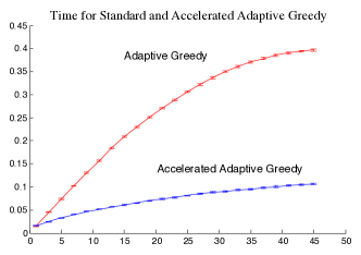
(a) Temperature Data: Execution time (sec) for the naive vs accelerated implementations of adaptive greedy vs. the budget $k$ on number of sensors selected, when $p_{\text{fail}}\!\left({v}\right)=0.5$ for all $v$, plotted with standard errors.

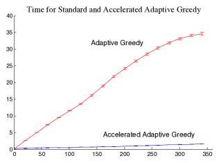
(b) Traffic Data: Execution time (sec) for the naive vs accelerated implementations of adaptive greedy vs. the budget $k$ on number of sensors selected, when $p_{\text{fail}}\!\left({v}\right)=0.5$ for all $v$, plotted with standard errors.

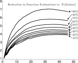
(c) Temperature Data: The ratio of function evaluations made by the naive vs accelerated implementations of adaptive greedy vs. the budget $k$ on number of sensors selected, for various failure rates. Averaged over $100$ runs.

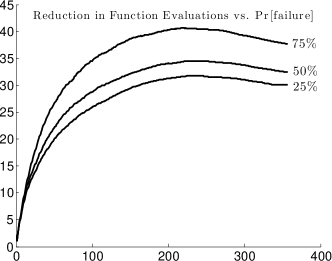
(d) Traffic Data: The ratio of function evaluations made by the naive vs accelerated implementations of adaptive greedy vs. the budget $k$ on number of sensors selected, for various failure rates. Averaged over $10$ runs.

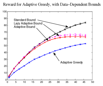
(e) Temperature Data: Rewards & bounds on the optimal value when $p_{\text{fail}}\!\left({v}\right)=0.5$ for all $v$ vs. the budget $k$ on number of sensors selected, plotted with standard errors.

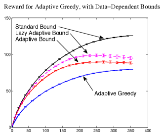
(f) Traffic Data: Rewards & bounds on the optimal value when $p_{\text{fail}}\!\left({v}\right)=0.5$ for all $v$ vs. the budget $k$ on number of sensors selected, plotted with standard errors.

Figure 5: Experimental results.

11 Adaptivity Gap

An important question in adaptive optimization is how much better adaptive policies can perform when compared to non-adaptive policies. This is quantified by the adaptivity gap, which is the worst-case ratio, over problem instances, of the performance of the optimal adaptive policy to the optimal non-adaptive solution. Asadpour et al. (2008) show that in the Stochastic Submodular Maximization problem with independent failures (as considered in §6), the expected value of the optimal non-adaptive policy is at most a constant factor $1-1/e$ worse than the expected value of the optimal adaptive policy. While we currently do not have lower bounds for the adaptivity gap of the general Adaptive Stochastic Maximization problem (1), we can show that even in the case of adaptive submodular functions, the min-cost cover and min-sum cover versions have large adaptivity gaps, and thus there is a large benefit of using adaptive algorithms. In these cases, the adaptivity gap is defined as the worst-case ratio of the expected cost of the optimal non-adaptive policy divided by the expected cost of the optimal adaptive policy. For the Adaptive Stochastic Minimum Cost Coverage problem (2), Goemans and Vondrák (2006) show the special case of Stochastic Set Coverage without multiplicities has an adaptivity gap of $\Omega(|E|)$. Below we exhibit an adaptive stochastic optimization instance with adaptivity gap of $\Omega(|E|/\log|E|)$ for the Adaptive Stochastic Min-Sum Cover problem (3), which also happens to have the same adaptivity gap for Adaptive Stochastic Minimum Cost Coverage.

Theorem 25

Even for adaptive submodular functions, the adaptivity gap of Adaptive Stochastic Min-Sum Cover is $\Omega(n/\log n)$, where $n=|E|$.

Proof  Suppose $E=\{1,\dots,n\}$. Consider the active learning problem where our hypotheses $h:E\rightarrow\left\{-1,1\right\}$ are threshold functions, i.e., $h(e)=1$ if $e\geq\ell$ and $h(e)=-1$ if $e<\ell$ for some threshold $\ell$. There is a uniform distribution over thresholds $\ell\in\{1,\dots,n+1\}$. In order to identify the correct hypothesis with threshold $\ell$, our policy must observe at least one of $\ell-1$ or $\ell$ (and both of them if $1<\ell\leq n$). Let $\hat{\pi}$ be an optimal non-adaptive policy for this problem. Note that $\hat{\pi}$ can be represented as a permutation of $E$, because observing an element multiple times can only increase the cost while providing no benefit over observing it once, and each element must eventually be selected to guarantee coverage. For the min-sum cover objective, consider playing $\hat{\pi}$ for $n/4$ time steps. Then $\mathbb{P}\left[\ell\text{ observed in }n/4\text{ steps}\right]=n/4(n+1)$. Likewise $\mathbb{P}\left[\ell-1\text{ observed in }n/4\text{ steps}\right]=n/4(n+1)$. Since at least one of these events must occur to identify the correct hypothesis, by a union bound

$$\mathbb{P}\left[\hat{\pi}\text{ identifies the correct hypothesis in }n/4\text{ steps}\right]\quad\leq\quad\frac{n}{2(n+1)}\quad\leq\quad 1/2.$$

Thus a lower bound on the expected cost of $\hat{\pi}$ is $n/8$, since for $n/4$ time steps a cost of at least $1/2$ is incurred. Thus, for both the min-cost and min-sum cover objectives the cost of the optimal non-adaptive policy is $\Omega(n)$.

As an example adaptive policy, we can implement a natural binary search strategy, which is guaranteed to identify the correct hypothesis after $O(\log n)$ steps, thus incurring cost $O(\log n)$, proving an adaptivity gap of $\Omega(n/\log n)$.  

12 Hardness of Approximation

In this paper, we have developed the notion of adaptive submodularity, which characterizes when certain adaptive stochastic optimization problems are well-behaved in the sense that a simple greedy policy obtains a constant factor or polylogarithmic factor approximation to the best policy.

In contrast, we can also show that without adaptive submodularity, the adaptive stochastic optimization problems (1), (2), and (3) are extremely inapproximable, even with (pointwise) modular objective functions (i.e., those where for each ${\color[rgb]{0,0,0}{\phi}}$, $f:2^{E}\times O^{E}\rightarrow\mathbb{R}$ is modular/linear in the first argument): We cannot hope to achieve an ${\mathcal{O}}(|E|^{1-\varepsilon})$ approximation ratio for these problems, unless the polynomial hierarchy collapses down to $\Sigma^{P}_{2}$.

Theorem 26

For all (possibly non-constant) $\beta\geq 1$, no polynomial time algorithm for Adaptive Stochastic Maximization with a budget of $\beta k$ items can approximate the reward of an optimal policy with a budget of only $k$ items to within a multiplicative factor of ${\mathcal{O}}(|E|^{1-\varepsilon}/\beta)$ for any $\varepsilon>0$, unless $\textrm{PH}=\Sigma^{P}_{2}$. This holds even for pointwise modular $f$.

We provide the proof of Theorem 26 in Appendix 15.7. Note that by setting $\beta=1$, we obtain ${\mathcal{O}}(|E|^{1-\varepsilon})$ hardness for Adaptive Stochastic Maximization. It turns out that in the instance distribution we construct in the proof of Theorem 26 the optimal policy covers every realization (i.e., always finds the treasure) using a budget of $k={\mathcal{O}}(|E|^{\varepsilon/2})$ items. Hence if $\textrm{PH}\neq\Sigma^{P}_{2}$ then any randomized polynomial time algorithm wishing to cover this instance must have a budget $\beta=\Omega(|E|^{1-\varepsilon})$ times larger than the optimal policy, in order to ensure the ratio of rewards, which is $\Omega(|E|^{1-\varepsilon}/\beta)$, equals one. This yields the following corollary.

Corollary 27

No polynomial time algorithm for Adaptive Stochastic Min Cost Coverage can approximate the cost of an optimal policy to within a multiplicative factor of ${\mathcal{O}}(|E|^{1-\varepsilon})$ for any $\varepsilon>0$, unless $\textrm{PH}=\Sigma^{P}_{2}$. This holds even for pointwise modular $f$.

Furthermore, since in the instance distribution we construct the optimal policy $\pi^{*}$ covers every realization using a budget of $k$, it has $c_{\Sigma}\!\left({\pi^{*}}\right)\leq k$. Moreover, since we have shown that under our complexity theoretic assumptions, any polynomial time randomized policy $\pi$ with budget $\beta k$ achieves at most $o(\beta/|E|^{1-\varepsilon})$ of the (unit) value obtained by the optimal policy with budget $k$, it follows that $c_{\Sigma}\!\left({\pi}\right)=\Omega(\beta k)$. Since we require $\beta=\Omega(|E|^{1-\varepsilon})$ to cover any set of realizations constituting, e.g., half of the probability mass, we obtain the following corollary.

Corollary 28

No polynomial time algorithm for Adaptive Stochastic Min-Sum Cover can approximate the cost of an optimal policy to within a multiplicative factor of ${\mathcal{O}}(|E|^{1-\varepsilon})$ for any $\varepsilon>0$, unless $\textrm{PH}=\Sigma^{P}_{2}$. This holds even for pointwise modular $f$.

13 Related Work

There is a large literature on adaptive optimization under partial observability which relates to adaptive submodularity, which can be broadly organized into several different categories. Here, we only review relevant related work that is not already discussed elsewhere in the manuscript.

13.1 Adaptive Versions of Classic Non-adaptive Optimization Problems

Many approaches consider stochastic generalizations of specific classic non-adaptive optimization problems, such as Set Cover (Goemans and Vondrák, 2006; Liu et al., 2008), Knapsack (Dean et al., 2008, 2005) and Traveling Salesman (Gupta et al., 2010). In contrast, in this paper our goal is to introduce a general problem structure – adaptive submodularity – that unifies a number of adaptive optimization problems. This is similar to how the classic notion of submodularity unifies various optimization problems such as Set Cover, Facility Location, nonadaptive Bayesian Experimental Design, etc.

13.2 Competitive Online Optimization

Another active area of research in sequential optimization is the study of competitive online algorithms. A particularly relevant example is Online Set Cover Alon et al. (2009), where there is a known set system, an arbitrary sequence of elements is presented to the algorithm, and the algorithm must irrevocably select sets to purchase such that at all times the purchased sets cover all elements which have appeared so far. Alon et al. (2009) obtain a polylogarithmic approximation to this problem, via an online primal–dual framework which has been profitably applied to many other problems. Buchbinder and Naor (2009) provide a detailed treatment of this framework. Note that competitive analysis focuses on worst–case scenarios. In contrast, we assume probabilistic information about the world and optimize for the average case.

13.3 (Noisy) Interactive Submodular Set Cover

Recent work by Guillory and Bilmes (2010); Guillory and Bilmes (2011) considers a class of adaptive optimization problems over a family of monotone submodular objectives $\left\{f_{h}:h\in H\right\}$. In their problem, one must cover a monotone submodular objective $f_{h^{*}}$ which depends on the (initially unknown) target hypothesis $h^{*}\in H$, by adaptively issuing queries and getting responses. Unlike traditional pool-based active learning, each query may generate a response from a set of valid responses depending on the target hypothesis. The reward is calculated by evaluating $f_{h^{*}}$ on the set of (query, response) pairs observed, and the goal is to obtain some threshold $Q$ of objective value at minimum total query cost, where queries may have nonuniform costs. In the noisy variant of the problem  (Guillory and Bilmes, 2011), the set of (query, response) pairs observed need not be consistent with any hypothesis in $H$, and the goal is to obtain $Q$ of value for all hypotheses that are “close” to being consistent with the observations. For both variants, Guillory and Bilmes consider the worst-case policy cost, and provide greedy algorithms optimizing clever hybrid objective functions. They prove an approximation guarantee of $\ln(Q|H|)+1$ for integer valued objective functions $\left\{f_{h}\right\}_{h\in H}$ in the noise–free case, and similar logarithmic approximation guarantees for the noisy case.

While similar in spirit to this work, there are several significant differences between the two. Guillory and Bilmes focus on worst-case policy cost, while we focus mainly on average-case policy cost. The structure of adaptive submodularity depends on the prior ${\color[rgb]{0,0,0}{p\left({{\color[rgb]{0,0,0}{\phi}}}\right)}}$, whereas there is no such dependence in Interactive Submodular Set Cover. This dependence in turn allows us to obtain results, such as Theorem 13 for self–certifying instances, whose approximation guarantee does not depend on the number of realizations in the way that the guarantees for Interactive Submodular Set Cover depend on $|H|$. As Guillory and Bilmes prove, the latter dependence is fundamental under reasonable complexity-theoretic assumptions. An interesting open problem within the adaptive submodularity framework that is highlighted by the work on Interactive Submodular Set Cover is to identify useful instance-specific properties that are sufficient to improve upon the worst-case approximation guarantee of Theorem 14.

13.4 Greedy Frameworks for Adaptive Optimization

The paper that is perhaps closest in spirit to this work is the one on Stochastic Depletion problems by Chan and Farias (2009), who also identify a general class of adaptive optimization problems than can be near-optimally solved using greedy algorithms (which in their setting give a factor 2 approximation). However, the similarity is mainly on a conceptual level: The problems and approaches, as well as example applications considered, are quite different.

13.5 Stochastic Optimization with Recourse

A class of adaptive optimization problems studied extensively in operations research since Dantzig (1955) is the area of stochastic optimization with recourse. Here, an optimization problem, such as Set Cover, Steiner Tree or Facility Location, is presented in multiple stages. At each stage, more information is revealed, but costs of actions increase. A key difference to the problems studied in this paper is that in these problems, information gets revealed independently of the actions taken by the algorithm. There are general efficient, sampling based (approximate) reductions of multi-stage optimization to the deterministic setting; see, e.g.,Gupta et al. (2005).

13.6 Bayesian Global Optimization

Adaptive Stochastic Optimization is also related to the problem of Bayesian Global Optimization (for a recent survey of the area, c.f. Brochu et al. (2009)). In Bayesian Global Optimization, the goal is to adaptively select inputs in order to maximize an unknown function that is expensive to evaluate (and can possibly only be evaluated using noisy observations). A common approach that has been successful in many applications (for a recent application in machine learning, c.f. Lizotte et al. (2007)), is to assume a prior distribution, such as a Gaussian process, over the unknown objective function. Several criteria for selecting inputs have been developed, such as the Expected Improvement (Jones et al., 1998) criterion. However, while recently performance guarantees where obtained in the no-regret setting (Grünewälder et al., 2010; Srinivas et al., 2010), we are not aware of any approximation guarantees for Bayesian Global Optimization.

13.7 Probabilistic Planning

The problem of decision making under partial observability has also been extensively studied in stochastic optimal control. In particular, Partially Observable Markov Decision Processes (Smallwood and Sondik, 1973), abbreviated as POMDPs, are a general framework that captures many adaptive optimization problems under partial observability. Unfortunately, solving POMDPs is PSPACE hard (Papadimitriou and Tsitsiklis, 1987), thus typically heuristic algorithms with no approximation guarantees are applied (Pineau et al., 2006; Ross et al., 2008). For some special instances of POMDPs related to Multi-armed Bandit problems, (near-)optimal policies can be found. These include the (optimal) Gittins-index policy for the classic Multi-armed Bandit problem (Gittins and Jones, 1979) and approximate policies for the Multi-armed Bandit problem with metric switching costs (Guha and Munagala, 2009) and special cases of the Restless Bandit problem (Guha et al., 2009). The problems considered in this paper can be formalized as POMDPs, albeit with exponentially large state space (where the world state represents the selected items and state/outcome of each item). Thus our results can be interpreted as widening the class of partially observable planning problems that can be efficiently approximately solved.

13.8 Previous Work by the Authors & Subsequent Developments

This manuscript is an extended version of a paper that appeared in the Conference on Learning Theory Golovin and Krause (2010). More recently, Golovin and Krause (2011b) proved performance guarantees for the greedy policy for the problem of maximizing the expected value of a policy under constraints more complex than simply selecting at most $k$ items. These include matroid constraints, where a policy can only select independent sets of items and the greedy policy obtains a $1/2$–approximation for adaptive monotone submodular objectives, and more generally $p$-independence system constraints, where the greedy policy obtains a $1/(p+1)$–approximation. Golovin et al. (2010) and, shortly thereafter, Bellala and Scott (2010), used the adaptive submodularity framework to obtain the first algorithms with provable (squared logarithmic) approximation guarantees for the difficult and fundamental problem of active learning with persistent noise. Finally, Golovin et al. (2011) used adaptive submodularity in the context of a dynamic conservation planning, and obtain competitiveness guarantees for an ecological reserve design problem.

14 Conclusions

Planning under partial observability is a central but notoriously difficult problem in artificial intelligence. In this paper, we identified a novel, general class of adaptive optimization problems under uncertainty that are amenable to efficient, greedy (approximate) solution. In particular, we introduced the concept of adaptive submodularity, generalizing submodular set functions to adaptive policies. Our generalization is based on a natural adaptive analog of the diminishing returns property well understood for set functions. In the special case of deterministic distributions, adaptive submodularity reduces to the classical notion of submodular set functions. We proved that several guarantees carried by the non-adaptive greedy algorithm for submodular set functions generalize to a natural adaptive greedy algorithm in the case of adaptive submodular functions, for constrained maximization and certain natural coverage problems with both minimum cost and minimum sum objectives. We also showed how the adaptive greedy algorithm can be accelerated using lazy evaluations, and how one can compute data-dependent bounds on the optimal solution. We illustrated the usefulness of the concept by giving several examples of adaptive submodular objectives arising in diverse AI applications including sensor placement, viral marketing, automated diagnosis and pool-based active learning. Proving adaptive submodularity for these problems allowed us to recover existing results in these applications as special cases and lead to natural generalizations. Our experiments on real data indicate that adaptive submodularity can provide practical benefits, such as significant speed ups and tighter data-dependent bounds. We believe that our results provide an interesting step in the direction of exploiting structure to solve complex stochastic optimization and planning problems under partial observability.

Acknowledgments

This research was partially supported by ONR grant N00014-09-1-1044, NSF grant CNS-0932392, NSF grant IIS-0953413, DARPA MSEE grant FA8650-11-1-7156, a gift by Microsoft Corporation, an Okawa Foundation Research Grant, and by the Caltech Center for the Mathematics of Information. We wish to thank Vitaly Feldman and Jan Vondrák for providing an elegant proof of Lemma 47.

15 Additional Proofs and Incorporating Item Costs

In this appendix we provide all of the proofs omitted from the main text. For the results of §5, we do so by first explaining how our results generalize to the case where items have costs, and then proving generalizations which incorporate item costs.

15.1 Incorporating Costs: Preliminaries

In this section we provide the preliminaries required to define and analyze the versions of our problems with non-uniform item costs. We suppose each item $e\in E$ has a cost $c(e)$, and the cost of a set $S\subseteq E$ is given by the modular function $c(S)=\sum_{e\in S}c(e)$. We define the generalizations of problems (1), (2), and (3) in §15.3, §15.4, and §15.5, respectively.

Our results are with respect to the greedy policy $\pi^{\text{greedy}}$ and $\alpha$-approximate greedy policies. With costs, the greedy policy selects an item maximizing $\Delta\left({{e}\!\mid\!{{\color[rgb]{0,0,0}{\psi}}}}\right)/c(e)$, where ${\color[rgb]{0,0,0}{\psi}}$ is the current partial realization.

Definition 29 (Approximate Greedy Policy with Costs)

A policy $\pi$ is an $\alpha$-approximate greedy policy if for all ${\color[rgb]{0,0,0}{\psi}}$ such that there exists $e\in E$ with $\Delta\left({{e}\!\mid\!{{\color[rgb]{0,0,0}{\psi}}}}\right)>0$,

$$\pi({\color[rgb]{0,0,0}{\psi}})\in\left\{e\ :\ \frac{\Delta\left({{e}\!\mid\!{{\color[rgb]{0,0,0}{\psi}}}}\right)}{c(e)}\ \geq\ \frac{1}{\alpha}\max_{e^{\prime}}\left({\frac{\Delta\left({{e^{\prime}}\!\mid\!{{\color[rgb]{0,0,0}{\psi}}}}\right)}{c(e^{\prime})}}\right)\right\},$$

and $\pi$ terminates upon observing any ${\color[rgb]{0,0,0}{\psi}}$ such that $\Delta\left({{e}\!\mid\!{{\color[rgb]{0,0,0}{\psi}}}}\right)\leq 0$ for all $e\in E$. That is, an $\alpha$-approximate greedy policy always obtains at least $(1/\alpha)$ of the maximum possible ratio of conditional expected marginal benefit to cost, and terminates when no more benefit can be obtained in expectation. A greedy policy is any $1$-approximate greedy policy.

It will be convenient to imagine the policy executing over time, such that when a policy $\pi$ selects an item $e$, it starts to run $e$, and finishes running $e$ after $c(e)$ units of time. We next generalize the definition of policy truncation. Actually we require three such generalizations, which are all equivalent in the unit cost case.

Definition 30 (Strict Policy Truncation)

The strict level $t$ truncation of a policy $\pi$, denoted by $\pi_{[\leftarrow{t}]}$, is obtained by running $\pi$ for $t$ time units, and unselecting items whose runs have not finished by time $t$. Formally, $\pi_{[\leftarrow{t}]}$ has domain $\left\{{\color[rgb]{0,0,0}{\psi}}\in\operatorname{dom}(\pi)\ :\ c(\pi({\color[rgb]{0,0,0}{\psi}}))+\sum_{e\in\operatorname{dom}({\color[rgb]{0,0,0}{\psi}})}c(e)\leq t\right\}$, and agrees with $\pi$ everywhere in its domain.

Definition 31 (Lax Policy Truncation)

The lax level $t$ truncation of a policy $\pi$, denoted by $\pi_{[{t}\to]}$, is obtained by running $\pi$ for $t$ time units, and selecting the items running at time $t$. Formally, $\pi_{[{t}\to]}$ has domain $\left\{{\color[rgb]{0,0,0}{\psi}}\in\operatorname{dom}(\pi)\ :\ \sum_{e\in\operatorname{dom}({\color[rgb]{0,0,0}{\psi}})}c(e)<t\right\}$, and agrees with $\pi$ everywhere in its domain.

Definition 32 (Policy Truncation with Costs)

The level-$t$-truncation of a policy $\pi$, denoted by $\pi_{[{t}]}$, is a randomized policy obtained by running $\pi$ for $t$ time units, and if some item $e$ has been running for $0\leq\tau<c(e)$ time at time $t$, selecting $e$ independently with probability $\tau/c(e)$. Formally, $\pi_{[{t}]}$ is a randomized policy that agrees with $\pi$ everywhere in its domain, has $\operatorname{dom}(\pi_{[\leftarrow{t}]})\subseteq\operatorname{dom}(\pi_{[{t}]})\subseteq\operatorname{dom}(\pi_{[{t}\to]})$ with certainty, and includes each ${\color[rgb]{0,0,0}{\psi}}\in\operatorname{dom}(\pi_{[{t}\to]})\setminus\operatorname{dom}(\pi_{[\leftarrow{t}]})$ in its domain independently with probability $\left({t-\sum_{e\in\operatorname{dom}({\color[rgb]{0,0,0}{\psi}})}c(e)}\right)/c(\pi({\color[rgb]{0,0,0}{\psi}}))$.

In the proofs that follow, we will need a notion of the conditional expected cost of a policy, as well as an alternate characterization of adaptive monotonicity, based on a notion of policy concatenation. We prove the equivalence of our two adaptive monotonicity conditions in Lemma 36.

Definition 33 (Conditional Policy Cost)

The conditional policy cost of $\pi$ conditioned on ${\color[rgb]{0,0,0}{\psi}}$, denoted $c\left({{\pi}\!\mid\!{{\color[rgb]{0,0,0}{\psi}}}}\right)$, is the expected cost of the items $\pi$ selects under ${\color[rgb]{0,0,0}{p\left({{\color[rgb]{0,0,0}{\phi}}\mid{\color[rgb]{0,0,0}{\psi}}}\right)}}$. That is, $c\left({{\pi}\!\mid\!{{\color[rgb]{0,0,0}{\psi}}}}\right):=\mathbb{E}\left[c(E({\pi},{{\color[rgb]{0,0,0}{\Phi}}}))\ \mid\ {\color[rgb]{0,0,0}{\Phi}}\sim{\color[rgb]{0,0,0}{\psi}}\right]$.

Definition 34 (Policy Concatenation)

Given two policies $\pi_{1}$ and $\pi_{2}$ define ${\pi_{1}}@{\pi_{2}}$ as the policy obtained by running $\pi_{1}$ to completion, and then running policy $\pi_{2}$ as if from a fresh start, ignoring the information gathered during the running of $\pi_{1}$.

Definition 35 (Adaptive Monotonicity (Alternate Version))

A function $f:2^{E}\times O^{E}\to\mathbb{R}_{\geq 0}$ is adaptive monotone with respect to distribution ${\color[rgb]{0,0,0}{p\left({{\color[rgb]{0,0,0}{\phi}}}\right)}}$ if for all policies $\pi$ and $\pi^{\prime}$, it holds that $f_{\text{avg}}(\pi)\leq f_{\text{avg}}({\pi^{\prime}}@{\pi})$, where $f_{\text{avg}}(\pi):=\mathbb{E}\left[f(E({\pi},{{\color[rgb]{0,0,0}{\Phi}}}),{\color[rgb]{0,0,0}{\Phi}})\right]$ is defined w.r.t. ${\color[rgb]{0,0,0}{p\left({{\color[rgb]{0,0,0}{\phi}}}\right)}}$.

Lemma 36 (Adaptive Monotonicity Equivalence)

Fix a function $f:2^{E}\times O^{E}\to\mathbb{R}_{\geq 0}$. Then $\Delta\left({{e}\!\mid\!{{\color[rgb]{0,0,0}{\psi}}}}\right)\geq 0$ for all ${\color[rgb]{0,0,0}{\psi}}$ with $\mathbb{P}\left[{\color[rgb]{0,0,0}{\Phi}}\sim{\color[rgb]{0,0,0}{\psi}}\right]>0$ and all $e\in E$ if and only if for all policies $\pi$ and $\pi^{\prime}$, $f_{\text{avg}}(\pi)\leq f_{\text{avg}}({\pi^{\prime}}@{\pi})$.

Proof  Fix policies $\pi$ and $\pi^{\prime}$. We begin by proving $f_{\text{avg}}({\pi^{\prime}}@{\pi})=f_{\text{avg}}({\pi}@{\pi^{\prime}})$. Fix any ${\color[rgb]{0,0,0}{\phi}}$ and note that $E({{\pi^{\prime}}@{\pi}},{{\color[rgb]{0,0,0}{\phi}}})=E({\pi^{\prime}},{{\color[rgb]{0,0,0}{\phi}}})\cup E({\pi},{{\color[rgb]{0,0,0}{\phi}}})=E({{\pi}@{\pi^{\prime}}},{{\color[rgb]{0,0,0}{\phi}}})$. Hence

$$f_{\text{avg}}({\pi^{\prime}}@{\pi})=\mathbb{E}\left[f(E({{\pi^{\prime}}@{\pi}},{{\color[rgb]{0,0,0}{\Phi}}}),{\color[rgb]{0,0,0}{\Phi}})\right]=\mathbb{E}\left[f(E({{\pi}@{\pi^{\prime}}},{{\color[rgb]{0,0,0}{\Phi}}}),{\color[rgb]{0,0,0}{\Phi}})\right]=f_{\text{avg}}({\pi}@{\pi^{\prime}}).$$

Therefore $f_{\text{avg}}(\pi)\leq f_{\text{avg}}({\pi^{\prime}}@{\pi})$ holds if and only if $f_{\text{avg}}(\pi)\leq f_{\text{avg}}({\pi}@{\pi^{\prime}})$.

We first prove the forward direction. Suppose $\Delta\left({{e}\!\mid\!{{\color[rgb]{0,0,0}{\psi}}}}\right)\geq 0$ for all ${\color[rgb]{0,0,0}{\psi}}$ and all $e\in E$. Note the expression $f_{\text{avg}}({\pi}@{\pi^{\prime}})-f_{\text{avg}}(\pi)$ can be written as a conical combination of (nonnegative) $\Delta\left({{e}\!\mid\!{{\color[rgb]{0,0,0}{\psi}}}}\right)$ terms, i.e., for some $\alpha\geq\mathbf{0}$, $f_{\text{avg}}({\pi}@{\pi^{\prime}})-f_{\text{avg}}(\pi)=\sum_{{\color[rgb]{0,0,0}{\psi}},e}\alpha_{({\color[rgb]{0,0,0}{\psi}},e)}\,\Delta\left({{e}\!\mid\!{{\color[rgb]{0,0,0}{\psi}}}}\right)$. Hence $f_{\text{avg}}({\pi}@{\pi^{\prime}})-f_{\text{avg}}(\pi)\geq 0$ and so $f_{\text{avg}}(\pi)\leq f_{\text{avg}}({\pi}@{\pi^{\prime}})=f_{\text{avg}}({\pi^{\prime}}@{\pi})$.

We next prove the backward direction, in contrapositive form. Suppose $\Delta\left({{e}\!\mid\!{{\color[rgb]{0,0,0}{\psi}}}}\right)<0$ for some ${\color[rgb]{0,0,0}{\psi}}$ with $\mathbb{P}\left[{\color[rgb]{0,0,0}{\Phi}}\sim{\color[rgb]{0,0,0}{\psi}}\right]>0$ and $e\in E$. Let $e_{1},\ldots,e_{r}$ be the items in $\operatorname{dom}({\color[rgb]{0,0,0}{\psi}})$ and define policies $\pi$ and $\pi^{\prime}$ as follows. For $i=1,2,\ldots,r$, both $\pi$ and $\pi^{\prime}$ select $e_{i}$ and observe ${\color[rgb]{0,0,0}{\Phi}}(e_{i})$. If either policy observes ${\color[rgb]{0,0,0}{\Phi}}(e_{i})\neq{\color[rgb]{0,0,0}{\psi}}(e_{i})$ it immediately terminates, otherwise it continues. If $\pi$ succeeds in selecting all of $\operatorname{dom}({\color[rgb]{0,0,0}{\psi}})$ then it terminates. If $\pi^{\prime}$ succeeds in selecting all of $\operatorname{dom}({\color[rgb]{0,0,0}{\psi}})$ then it selects $e$ and then terminates. We claim $f_{\text{avg}}({\pi}@{\pi^{\prime}})-f_{\text{avg}}(\pi)<0$. Note that $E({{\pi}@{\pi^{\prime}}},{{\color[rgb]{0,0,0}{\phi}}})=E({\pi},{{\color[rgb]{0,0,0}{\phi}}})$ unless ${\color[rgb]{0,0,0}{\phi}}\sim{\color[rgb]{0,0,0}{\psi}}$, and if ${\color[rgb]{0,0,0}{\phi}}\sim{\color[rgb]{0,0,0}{\psi}}$ then $E({{\pi}@{\pi^{\prime}}},{{\color[rgb]{0,0,0}{\phi}}})=E({\pi},{{\color[rgb]{0,0,0}{\phi}}})\cup\left\{e\right\}$ and also $E({\pi},{{\color[rgb]{0,0,0}{\phi}}})=\operatorname{dom}({\color[rgb]{0,0,0}{\psi}})$. Hence

$$f_{\text{avg}}({\pi}@{\pi^{\prime}})-f_{\text{avg}}(\pi) = \mathbb{E}\left[f(E({{\pi}@{\pi^{\prime}}},{{\color[rgb]{0,0,0}{\Phi}}}),{\color[rgb]{0,0,0}{\Phi}})-f(E({\pi},{{\color[rgb]{0,0,0}{\Phi}}}),{\color[rgb]{0,0,0}{\Phi}})\right]$$

$$= \mathbb{E}\left[f(E({{\pi}@{\pi^{\prime}}},{{\color[rgb]{0,0,0}{\Phi}}}),{\color[rgb]{0,0,0}{\Phi}})-f(E({\pi},{{\color[rgb]{0,0,0}{\Phi}}}),{\color[rgb]{0,0,0}{\Phi}})\ |\ {\color[rgb]{0,0,0}{\Phi}}\sim{\color[rgb]{0,0,0}{\psi}}\right]\cdot\mathbb{P}\left[{\color[rgb]{0,0,0}{\Phi}}\sim{\color[rgb]{0,0,0}{\psi}}\right]$$

$$= \mathbb{E}\left[f(\operatorname{dom}({\color[rgb]{0,0,0}{\psi}})\cup\left\{e\right\},{\color[rgb]{0,0,0}{\Phi}})-f(\operatorname{dom}({\color[rgb]{0,0,0}{\psi}}),{\color[rgb]{0,0,0}{\Phi}})\ |\ {\color[rgb]{0,0,0}{\Phi}}\sim{\color[rgb]{0,0,0}{\psi}}\right]\cdot\mathbb{P}\left[{\color[rgb]{0,0,0}{\Phi}}\sim{\color[rgb]{0,0,0}{\psi}}\right]$$

$$= \Delta\left({{e}\!\mid\!{{\color[rgb]{0,0,0}{\psi}}}}\right)\cdot\mathbb{P}\left[{\color[rgb]{0,0,0}{\Phi}}\sim{\color[rgb]{0,0,0}{\psi}}\right]$$

The last term is negative, as $\mathbb{P}\left[{\color[rgb]{0,0,0}{\Phi}}\sim{\color[rgb]{0,0,0}{\psi}}\right]>0$ and $\Delta\left({{e}\!\mid\!{{\color[rgb]{0,0,0}{\psi}}}}\right)<0$ by assumption. Therefore $f_{\text{avg}}(\pi)>f_{\text{avg}}({\pi}@{\pi^{\prime}})=f_{\text{avg}}({\pi^{\prime}}@{\pi})$, which completes the proof.  

15.2 Adaptive Data Dependent Bounds with Costs

The adaptive data dependent bound has the following generalization with costs.

Lemma 37 (The Adaptive Data Dependent Bound with Costs)

Suppose we have made observations ${\color[rgb]{0,0,0}{\psi}}$ after selecting $\operatorname{dom}({\color[rgb]{0,0,0}{\psi}})$. Let $\pi^{*}$ be any policy. Then for adaptive monotone submodular $f:2^{E}\times O^{E}\to\mathbb{R}_{\geq 0}$

$$\Delta\left({{\pi^{*}}\!\mid\!{{\color[rgb]{0,0,0}{\psi}}}}\right)\ \leq\ Z\ \leq\ c\left({{\pi^{*}}\!\mid\!{{\color[rgb]{0,0,0}{\psi}}}}\right)\max_{e}\left({\frac{\Delta\left({{e}\!\mid\!{{\color[rgb]{0,0,0}{\psi}}}}\right)}{c(e)}}\right)$$ (30)

where $Z=\max_{w}\left\{\sum_{e\in E}w_{e}\,\Delta\left({{e}\!\mid\!{{\color[rgb]{0,0,0}{\psi}}}}\right)\ :\ \sum_{e}c(e)w_{e}\leq c\left({{\pi^{*}}\!\mid\!{{\color[rgb]{0,0,0}{\psi}}}}\right)\text{ and }\forall e\in E,0\leq w_{e}\leq 1\right\}$.

Proof  Order the items in $\operatorname{dom}({\color[rgb]{0,0,0}{\psi}})$ arbitrarily, and consider the policy $\pi$ that for each $e\in\operatorname{dom}({\color[rgb]{0,0,0}{\psi}})$ in order selects $e$, terminating if ${\color[rgb]{0,0,0}{\Phi}}(e)\neq{\color[rgb]{0,0,0}{\psi}}(e)$ and proceeding otherwise, and, should it succeed in selecting all of $\operatorname{dom}({\color[rgb]{0,0,0}{\psi}})$ without terminating (which occurs iff ${\color[rgb]{0,0,0}{\Phi}}\sim{\color[rgb]{0,0,0}{\psi}}$), then proceeds to run $\pi^{*}$ as if from a fresh start, forgetting the observations in ${\color[rgb]{0,0,0}{\psi}}$. By construction the expected marginal benefit of running the $\pi^{*}$ portion of $\pi$ conditioned on ${\color[rgb]{0,0,0}{\Phi}}\sim{\color[rgb]{0,0,0}{\psi}}$ equals $\Delta\left({{\pi^{*}}\!\mid\!{{\color[rgb]{0,0,0}{\psi}}}}\right)$. For all $e\in E$, let $w(e)=\mathbb{P}\left[e\in E({\pi},{{\color[rgb]{0,0,0}{\Phi}}})\ \mid\ {\color[rgb]{0,0,0}{\Phi}}\sim{\color[rgb]{0,0,0}{\psi}}\right]$ be the probability that $e$ is selected when running $\pi$, conditioned on ${\color[rgb]{0,0,0}{\Phi}}\sim{\color[rgb]{0,0,0}{\psi}}$. Whenever some $e\in E\setminus\operatorname{dom}({\color[rgb]{0,0,0}{\psi}})$ is selected by $\pi$, the current partial realization ${\color[rgb]{0,0,0}{\psi}}^{\prime}$ contains ${\color[rgb]{0,0,0}{\psi}}$ as a subrealization; hence adaptive submodularity implies $\Delta\left({{e}\!\mid\!{{\color[rgb]{0,0,0}{\psi}}^{\prime}}}\right)\leq\Delta\left({{e}\!\mid\!{{\color[rgb]{0,0,0}{\psi}}}}\right)$. It follows that the total contribution of $e$ to $\Delta\left({{\pi^{*}}\!\mid\!{{\color[rgb]{0,0,0}{\psi}}}}\right)$ is upper bounded by $w(e)\cdot\Delta\left({{e}\!\mid\!{{\color[rgb]{0,0,0}{\psi}}}}\right)$. Summing over $e\in E\setminus\operatorname{dom}({\color[rgb]{0,0,0}{\psi}})$, we get a bound of $\Delta\left({{\pi^{*}}\!\mid\!{{\color[rgb]{0,0,0}{\psi}}}}\right)\leq\sum_{e\in E\setminus\operatorname{dom}({\color[rgb]{0,0,0}{\psi}})}w(e)\Delta\left({{e}\!\mid\!{{\color[rgb]{0,0,0}{\psi}}}}\right)$. Next, note that each $e\in E\setminus\operatorname{dom}({\color[rgb]{0,0,0}{\psi}})$ contributes $w(e)c(e)$ cost to $c\left({{\pi^{*}}\!\mid\!{{\color[rgb]{0,0,0}{\psi}}}}\right)$. Hence it must be the case that $\sum_{e\in E\setminus\operatorname{dom}({\color[rgb]{0,0,0}{\psi}})}w(e)c(e)\leq c\left({{\pi^{*}}\!\mid\!{{\color[rgb]{0,0,0}{\psi}}}}\right)$. Obviously, $w(e)\in[0,1]$ for all $e$, since $w(e)$ is a probability. Hence $\Delta\left({{\pi^{*}}\!\mid\!{{\color[rgb]{0,0,0}{\psi}}}}\right)\leq\sum_{e\in E\setminus\operatorname{dom}({\color[rgb]{0,0,0}{\psi}})}w(e)\Delta\left({{e}\!\mid\!{{\color[rgb]{0,0,0}{\psi}}}}\right)\leq Z$ because setting $w_{e}=w(e)$ is feasible for the the linear program for which $Z$ is the optimal value.

To show $Z\leq c\left({{\pi^{*}}\!\mid\!{{\color[rgb]{0,0,0}{\psi}}}}\right)\max_{e}\left({\Delta\left({{e}\!\mid\!{{\color[rgb]{0,0,0}{\psi}}}}\right)/c(e)}\right)$, consider any feasible solution $w$ to the linear program defining $Z$. It attains objective value

$$\sum_{e\in E}w_{e}\,\Delta\left({{e}\!\mid\!{{\color[rgb]{0,0,0}{\psi}}}}\right)\leq\sum_{e\in E}w_{e}c(e)\frac{\Delta\left({{e}\!\mid\!{{\color[rgb]{0,0,0}{\psi}}}}\right)}{c(e)}\leq\sum_{e\in E}w_{e}c(e)\max_{e\in E}\left({\frac{\Delta\left({{e}\!\mid\!{{\color[rgb]{0,0,0}{\psi}}}}\right)}{c(e)}}\right)\leq c\left({{\pi^{*}}\!\mid\!{{\color[rgb]{0,0,0}{\psi}}}}\right)\max_{e\in E}\left({\frac{\Delta\left({{e}\!\mid\!{{\color[rgb]{0,0,0}{\psi}}}}\right)}{c(e)}}\right)$$

since $\sum_{e\in E}w_{e}c(e)\leq c\left({{\pi^{*}}\!\mid\!{{\color[rgb]{0,0,0}{\psi}}}}\right)$ by the feasibility of $w$.  

A simple greedy algorithm can be used to compute $Z$; we provide pseudocode for it in Algorithm 3. The correctness of this algorithm is more readily discerned upon rewriting the linear program using variables $x_{e}=c(e)w_{e}$ to obtain

$$Z=\max_{x}\left\{\sum_{e\in E}x_{e}\left({\Delta\left({{e}\!\mid\!{{\color[rgb]{0,0,0}{\psi}}}}\right)/c(e)}\right)\ :\ \sum_{e}x_{e}\leq c\left({{\pi^{*}}\!\mid\!{{\color[rgb]{0,0,0}{\psi}}}}\right)\text{ and }\forall e\in E,0\leq x_{e}\leq c(e)\right\}.$$

Intuitively, it is clear that to optimize $x$ we should shift mass towards variables with the highest $\Delta\left({{e}\!\mid\!{{\color[rgb]{0,0,0}{\psi}}}}\right)/c(e)$ ratio. Clearly, any optimal solution has $\sum_{e}x_{e}=c\left({{\pi^{*}}\!\mid\!{{\color[rgb]{0,0,0}{\psi}}}}\right)$. Moreover, in any optimal solution, $\Delta\left({{e}\!\mid\!{{\color[rgb]{0,0,0}{\psi}}}}\right)/c(e)>\Delta\left({{e^{\prime}}\!\mid\!{{\color[rgb]{0,0,0}{\psi}}}}\right)/c(e^{\prime})$ implies $x_{e}=c(e)$ or $x_{e^{\prime}}=0$, since otherwise it would be possible to shift mass from $x_{e^{\prime}}$ to $x_{e}$ and obtain an increase in objective value. If the $\Delta\left({{e}\!\mid\!{{\color[rgb]{0,0,0}{\psi}}}}\right)/c(e)$ values are distinct for distinct items, there will be a unique solution satisfying these constraints, which Algorithm 3 will compute. Otherwise, we imagine perturbing each $\Delta\left({{e}\!\mid\!{{\color[rgb]{0,0,0}{\psi}}}}\right)$ by independent random quantities $\epsilon_{e}$ drawn uniformly from $[0,\epsilon]$ to make them distinct. This changes the optimum value by at most $|E|\epsilon$, which vanishes as we let $\epsilon$ tend towards zero. Hence any solution satisfying $\sum_{e}x_{e}=c\left({{\pi^{*}}\!\mid\!{{\color[rgb]{0,0,0}{\psi}}}}\right)$ and $\Delta\left({{e}\!\mid\!{{\color[rgb]{0,0,0}{\psi}}}}\right)/c(e)>\Delta\left({{e^{\prime}}\!\mid\!{{\color[rgb]{0,0,0}{\psi}}}}\right)/c(e^{\prime})$ implies $x_{e}=c(e)$ or $x_{e^{\prime}}=0$ is optimal. Since Algorithm 3 outputs the value of such a solution, it is correct.

Input: Groundset $E$; Partial realization ${\color[rgb]{0,0,0}{\psi}}$; Costs $c:E\to\mathbb{N}$; Budget $C=c\left({{\pi^{*}}\!\mid\!{{\color[rgb]{0,0,0}{\psi}}}}\right)$; Conditional expected marginal benefits $\Delta\left({{e}\!\mid\!{{\color[rgb]{0,0,0}{\psi}}}}\right)$ for all $e\in E$.

Output: $Z=\max_{w}\left\{\sum_{e\in E}w_{e}\,\Delta\left({{e}\!\mid\!{{\color[rgb]{0,0,0}{\psi}}}}\right)\ :\ \sum_{e}c(e)w_{e}\leq c\left({{\pi^{*}}\!\mid\!{{\color[rgb]{0,0,0}{\psi}}}}\right)\text{ and }\forall e\in E,0\leq w_{e}\leq 1\right\}$

begin Sort $E$ by $\Delta\left({{e}\!\mid\!{{\color[rgb]{0,0,0}{\psi}}}}\right)/c(e)$, so that $\frac{\Delta\left({{e_{1}\ }\!\mid\!{\ {\color[rgb]{0,0,0}{\psi}}}}\right)}{c(e_{1})}\geq\frac{\Delta\left({{e_{2}\ }\!\mid\!{\ {\color[rgb]{0,0,0}{\psi}}}}\right)}{c(e_{2})}\geq\ldots\geq\frac{\Delta\left({{e_{n}\ }\!\mid\!{\ {\color[rgb]{0,0,0}{\psi}}}}\right)}{c(e_{n})}$;

Set $w\leftarrow\mathbf{0}$; $i\leftarrow 0$; $a\leftarrow 0$; $z\leftarrow 0$; $e\leftarrow\textsc{null}$;

while $a<C$ do $i\leftarrow i+1$;    $e\leftarrow e_{i}$;

$w_{e}\leftarrow\min\left\{1,C-a\right\}$;

$a\leftarrow a+c(e)w_{e}$;   $z\leftarrow z+w_{e}\Delta\left({{e}\!\mid\!{{\color[rgb]{0,0,0}{\psi}}}}\right)$; Output $z$; end

Algorithm 3 Algorithm to compute the data dependent bound $Z$ of Lemma 37.

15.3 The Max-Cover Objective

With item costs, the Adaptive Stochastic Maximization problem becomes one of finding some

$$\pi^{*}\in\mathop{\rm arg\,max}_{\pi}f_{\text{avg}}(\pi_{[{k}]})$$ (31)

where $k$ is a budget on the cost of selected items, and we define $f_{\text{avg}}(\pi)$ for a randomized policy $\pi$ to be $f_{\text{avg}}(\pi):=\mathbb{E}\left[f(E({\pi},{{\color[rgb]{0,0,0}{\Phi}}}),{\color[rgb]{0,0,0}{\Phi}})\right]$ as before, where the expectation is now over both ${\color[rgb]{0,0,0}{\Phi}}$ and the internal randomness of $\pi$ which determines $E({\pi},{{\color[rgb]{0,0,0}{\phi}}})$ for each ${\color[rgb]{0,0,0}{\phi}}$. We prove the following generalization of Theorem 5.

Theorem 38

Fix any $\alpha\geq 1$ and item costs $c:E\to\mathbb{N}$. If $f$ is adaptive monotone and adaptive submodular with respect to the distribution ${\color[rgb]{0,0,0}{p\left({{\color[rgb]{0,0,0}{\phi}}}\right)}}$, and $\pi$ is an $\alpha$-approximate greedy policy, then for all policies $\pi^{*}$ and positive integers $\ell$ and $k$

$$f_{\text{avg}}(\pi_{[{\ell}]})>\left({1-e^{-\ell/\alpha k}}\right)f_{\text{avg}}(\pi^{*}_{[{k}]})\mbox{.}$$

Proof  The proof goes along the lines of the performance analysis of the greedy algorithm for maximizing a submodular function subject to a cardinality constraint of Nemhauser et al. (1978). An extension of that analysis to $\alpha$-approximate greedy algorithms, which is analogous to ours but for the nonadaptive case, is shown by Goundan and Schulz (2007). For brevity, we will assume without loss of generality that $\pi=\pi_{[{\ell}]}$ and $\pi^{*}=\pi^{*}_{[{k}]}$. Then for all $i$, $0\leq i<\ell$

$$f_{\text{avg}}(\pi^{*})\ \ \leq\ \ f_{\text{avg}}({\pi_{[{i}]}}@{\pi^{*}})\ \ \leq\ \ f_{\text{avg}}(\pi_{[{i}]})+\alpha k\left({f_{\text{avg}}(\pi_{[{i+1}]})-f_{\text{avg}}(\pi_{[{i}]})}\right).$$ (32)

The first inequality is due to the adaptive monotonicity of $f$ and Lemma 36, from which we may infer $f_{\text{avg}}(\pi_{2})\leq f_{\text{avg}}({\pi_{1}}@{\pi_{2}})$ for any $\pi_{1}$ and $\pi_{2}$. The second inequality may be obtained as a corollary of Lemma 37 as follows. Fix any partial realization ${\color[rgb]{0,0,0}{\psi}}$ of the form $\left\{(e,{\color[rgb]{0,0,0}{\phi}}(e)):e\in E({\pi_{[{i}]}},{{\color[rgb]{0,0,0}{\phi}}})\right\}$ for some ${\color[rgb]{0,0,0}{\phi}}$. Consider $\Delta\left({{\pi^{*}}\!\mid\!{{\color[rgb]{0,0,0}{\psi}}}}\right)$, which equals the expected marginal benefit of the $\pi^{*}$ portion of ${\pi_{[{i}]}}@{\pi^{*}}$ conditioned on ${\color[rgb]{0,0,0}{\Phi}}\sim{\color[rgb]{0,0,0}{\psi}}$. Lemma 37 allows us to bound it as

$$\mathbb{E}\left[\Delta\left({{\pi^{*}}\!\mid\!{{\color[rgb]{0,0,0}{\psi}}}}\right)\right]\ \leq\ \mathbb{E}\left[c\left({{\pi^{*}}\!\mid\!{{\color[rgb]{0,0,0}{\psi}}}}\right)\right]\cdot\max_{e}\left({\Delta\left({{e}\!\mid\!{{\color[rgb]{0,0,0}{\psi}}}}\right)/c(e)}\right),$$

where the expectations are taken over the internal randomness of $\pi^{*}$, if there is any. Note that since $\pi^{*}$ has the form $\pi^{\prime}_{[{k}]}$ for some $\pi^{\prime}$ we know that for all ${\color[rgb]{0,0,0}{\phi}}$, $\mathbb{E}\left[c(E({\pi^{*}},{{\color[rgb]{0,0,0}{\phi}}}))\right]\leq k$, where the expectation is again taken over the internal randomness of $\pi^{*}$. Hence $\mathbb{E}\left[c\left({{\pi^{*}}\!\mid\!{{\color[rgb]{0,0,0}{\psi}}}}\right)\right]\leq k$ for all ${\color[rgb]{0,0,0}{\psi}}$. It follows that $\mathbb{E}\left[\Delta\left({{\pi^{*}}\!\mid\!{{\color[rgb]{0,0,0}{\psi}}}}\right)\right]\leq k\cdot\max_{e}\left({\Delta\left({{e}\!\mid\!{{\color[rgb]{0,0,0}{\psi}}}}\right)/c(e)}\right)$. By definition of an $\alpha$-approximate greedy policy, $\pi$ obtains at least $(1/\alpha)\max_{e}\left({\Delta\left({{e}\!\mid\!{{\color[rgb]{0,0,0}{\psi}}}}\right)/c(e)}\right)\geq\mathbb{E}\left[\Delta\left({{\pi^{*}}\!\mid\!{{\color[rgb]{0,0,0}{\psi}}}}\right)\right]/\alpha k$ expected marginal benefit per unit cost in a step immediately following its observation of ${\color[rgb]{0,0,0}{\psi}}$. Next we take an appropriate convex combination of the previous inequality with different values of ${\color[rgb]{0,0,0}{\psi}}$. Let ${\color[rgb]{0,0,0}{\Psi}}$ be a random partial realization distributed as ${\color[rgb]{0,0,0}{p_{{\color[rgb]{0,0,0}{\Psi}}}\!\left({{\color[rgb]{0,0,0}{\psi}}}\right)}}:=\mathbb{P}\left[{\color[rgb]{0,0,0}{\Psi}}={\color[rgb]{0,0,0}{\psi}}\mid\exists{\color[rgb]{0,0,0}{\phi}}.\ {\color[rgb]{0,0,0}{\psi}}=\left\{(e,{\color[rgb]{0,0,0}{\phi}}(e)):e\in E({\pi_{[{i}]}},{{\color[rgb]{0,0,0}{\phi}}})\right\}\right]$ Then

$$f_{\text{avg}}(\pi_{[{i+1}]})-f_{\text{avg}}(\pi_{[{i}]}) \geq \mathbb{E}\left[\frac{1}{\alpha}\,\max_{e}\left({\frac{\Delta\left({{e}\!\mid\!{{\color[rgb]{0,0,0}{\Psi}}}}\right)}{c(e)}}\right)\right]$$

$$\geq \mathbb{E}\left[\frac{\mathbb{E}\left[\Delta\left({{\pi^{*}}\!\mid\!{{\color[rgb]{0,0,0}{\Psi}}}}\right)\right]}{\alpha k}\right]$$

$$= \frac{f_{\text{avg}}({\pi_{[{i}]}}@{\pi^{*}})-f_{\text{avg}}(\pi_{[{i}]})}{\alpha k}$$

A simple rearrangement of terms then yields the second inequality in (32).

Now define $\Delta_{i}:=f_{\text{avg}}(\pi^{*})-f_{\text{avg}}(\pi_{[{i}]})$, so that (32) implies $\Delta_{i}\leq\alpha k(\Delta_{i}-\Delta_{i+1})$, from which we infer $\Delta_{i+1}\leq\left({1-\frac{1}{\alpha k}}\right)\Delta_{i}$ and hence $\Delta_{\ell}\leq\left({1-\frac{1}{\alpha k}}\right)^{\ell}\Delta_{0}<e^{-\ell/\alpha k}\Delta_{0}$, where for this last inequality we have used the fact that $1-x<e^{-x}$ for all $x>0$. Thus $f_{\text{avg}}(\pi^{*})-f_{\text{avg}}(\pi_{[{\ell}]})<e^{-\ell/\alpha k}\left({f_{\text{avg}}(\pi^{*})-f_{\text{avg}}(\pi_{[{0}]})}\right)\leq e^{-\ell/\alpha k}f_{\text{avg}}(\pi^{*})$ so $f_{\text{avg}}(\pi)>(1-e^{-\ell/\alpha k})f_{\text{avg}}(\pi^{*})$.

 

15.4 The Min-Cost-Cover Objective

In this section, we provide arbitrary item cost generalizations of Theorem 13 and Theorem 14. With item costs the Adaptive Stochastic Minimum Cost Cover problem becomes one of finding, for some quota on utility $Q$,

$$\pi^{*}\in\mathop{\rm arg\,min}_{\pi}{c_{\text{avg}}{(\pi)}}\text{ such that }f(E({\pi},{{\color[rgb]{0,0,0}{\phi}}}),{\color[rgb]{0,0,0}{\phi}})\geq Q\text{ for all }{\color[rgb]{0,0,0}{\phi}},$$ (33)

where ${c_{\text{avg}}{(\pi)}}:=\mathbb{E}\left[c(E({\pi},{{\color[rgb]{0,0,0}{\Phi}}}))\right]$. Without loss of generality, we may take a truncated version of $f$, namely $(A,{\color[rgb]{0,0,0}{\phi}})\mapsto\min\left\{Q,f(A,{\color[rgb]{0,0,0}{\phi}})\right\}$, and rephrase Problem (33) as finding

$$\pi^{*}\in\mathop{\rm arg\,min}_{\pi}{c_{\text{avg}}{(\pi)}}\text{ such that }\pi\text{ covers }{\color[rgb]{0,0,0}{\phi}}\text{ for all }{\color[rgb]{0,0,0}{\phi}}.$$ (34)

Hereby, recall that $\pi$ covers ${\color[rgb]{0,0,0}{\phi}}$ if $\mathbb{E}\left[f(E({\pi},{{\color[rgb]{0,0,0}{\phi}}}),{\color[rgb]{0,0,0}{\phi}})\right]=f(E,{\color[rgb]{0,0,0}{\phi}})$, where the expectation is over any internal randomness of $\pi$. We will consider only Problem (34) for the remainder. We also consider the worst-case variant of this problem, where we replace the expected cost ${c_{\text{avg}}{(\pi)}}$ objective with the worst-case cost ${c_{\text{wc}}{(\pi)}}:=\max_{{\color[rgb]{0,0,0}{\phi}}}{c(E({\pi},{{\color[rgb]{0,0,0}{\phi}}}))}$.

The definition of coverage (Definition 7 in §5.2 on page 7) requires no modification to handle item costs. Note, however, that coverage is all-or-nothing in the sense that covering a realization ${\color[rgb]{0,0,0}{\phi}}$ with probability less than one does not count as covering it. A corollary of this is that only items whose runs have finished help with coverage, whereas currently running items do not. For a simple example, consider the case where $E=\left\{e\right\}$, $c(e)=2$, $f(A,{\color[rgb]{0,0,0}{\phi}})=|A|$, and policy $\pi$ that selects $e$ and then terminates. Then $\pi_{[{1}]}$ is a randomized policy which is $\pi$ with probability $\frac{1}{2}$, and is the empty policy with probability $\frac{1}{2}$, so $\mathbb{E}\left[f(E({\pi},{{\color[rgb]{0,0,0}{\phi}}}),{\color[rgb]{0,0,0}{\phi}})\right]=\frac{1}{2}<1=f(E,{\color[rgb]{0,0,0}{\phi}})$ for each ${\color[rgb]{0,0,0}{\phi}}$. Hence, even though half the time $\pi_{[{1}]}$ covers all realizations, it is counted as not covering any.

We begin with a claim relating pointwise submodularity to strong adaptive submodularity.

Lemma 39

If $f$ is adaptive submodular with respect to ${\color[rgb]{0,0,0}{p\left({{\color[rgb]{0,0,0}{\phi}}}\right)}}$ and $f$ is pointwise submodular meaning $S\mapsto f(S,{\color[rgb]{0,0,0}{\phi}})$ is submodular for all ${\color[rgb]{0,0,0}{\phi}}$, then $f$ is strongly adaptive submodular with respect to ${\color[rgb]{0,0,0}{p\left({{\color[rgb]{0,0,0}{\phi}}}\right)}}$.

Proof  By assumption $f$ is adaptive submodular with respect to ${\color[rgb]{0,0,0}{p\left({{\color[rgb]{0,0,0}{\phi}}}\right)}}$, so it is sufficient to prove that Eq. (16) holds, i.e., $\Delta\left({{e}\!\mid\!{{\color[rgb]{0,0,0}{\psi}};{\color[rgb]{0,0,0}{\psi}}^{\prime}}}\right)\geq\Delta\left({{e}\!\mid\!{{\color[rgb]{0,0,0}{\psi}}^{\prime}}}\right)$. Fix any ${\color[rgb]{0,0,0}{\psi}}\subseteq{\color[rgb]{0,0,0}{\psi}}^{\prime}$ and $e\in E$. Let $\delta_{{\color[rgb]{0,0,0}{\phi}}}(e,S):=f(S\cup\left\{e\right\},{\color[rgb]{0,0,0}{\phi}})-f(S,{\color[rgb]{0,0,0}{\phi}})$. From the definition of $\Delta\left({{e}\!\mid\!{{\color[rgb]{0,0,0}{\psi}};{\color[rgb]{0,0,0}{\psi}}^{\prime}}}\right)$ and $\Delta\left({{e}\!\mid\!{{\color[rgb]{0,0,0}{\psi}}^{\prime}}}\right)$, we have

$$\Delta\left({{e}\!\mid\!{{\color[rgb]{0,0,0}{\psi}};{\color[rgb]{0,0,0}{\psi}}^{\prime}}}\right) = \sum_{{\color[rgb]{0,0,0}{\phi}}}\mathbb{P}\left[{\color[rgb]{0,0,0}{\phi}}\mid{\color[rgb]{0,0,0}{\psi}}^{\prime}\right]\delta_{{\color[rgb]{0,0,0}{\phi}}}(e,\operatorname{dom}({\color[rgb]{0,0,0}{\psi}}))$$

$$\geq \sum_{{\color[rgb]{0,0,0}{\phi}}}\mathbb{P}\left[{\color[rgb]{0,0,0}{\phi}}\mid{\color[rgb]{0,0,0}{\psi}}^{\prime}\right]\delta_{{\color[rgb]{0,0,0}{\phi}}}(e,\operatorname{dom}({\color[rgb]{0,0,0}{\psi}}^{\prime}))$$

$$= \Delta\left({{e}\!\mid\!{{\color[rgb]{0,0,0}{\psi}}^{\prime}}}\right)$$

where we have used $\delta_{{\color[rgb]{0,0,0}{\phi}}}(e,\operatorname{dom}({\color[rgb]{0,0,0}{\psi}}))\geq\delta_{{\color[rgb]{0,0,0}{\phi}}}(e,\operatorname{dom}({\color[rgb]{0,0,0}{\psi}}^{\prime}))$ by the pointwise submodularity of $f$.  

Now we provide an approximation guarantee for the average-case policy cost with arbitrary item costs.

Theorem 40

Suppose $f:2^{E}\times O^{E}\to\mathbb{R}_{\geq 0}$ is strongly adaptive submodular and strongly adaptive monotone with respect to ${\color[rgb]{0,0,0}{p\left({{\color[rgb]{0,0,0}{\phi}}}\right)}}$ and there exists $Q$ such that $f(E,{\color[rgb]{0,0,0}{\phi}})=Q$ for all ${\color[rgb]{0,0,0}{\phi}}$. Let $\eta$ be any value such that $f(S,{\color[rgb]{0,0,0}{\phi}})>Q-\eta$ implies $f(S,{\color[rgb]{0,0,0}{\phi}})=Q$ for all $S$ and ${\color[rgb]{0,0,0}{\phi}}$. Let $\delta=\min_{{\color[rgb]{0,0,0}{\phi}}}{\color[rgb]{0,0,0}{p\left({{\color[rgb]{0,0,0}{\phi}}}\right)}}$ be the minimum probability of any realization. Let $\pi_{\text{avg}}^{*}$ be an optimal policy minimizing the expected cost of items selected to guarantee every realization is covered. Let $\pi$ be an $\alpha$-approximate greedy policy with respect to the item costs. Then in general

$${c_{\text{avg}}{(\pi)}}\leq\alpha\,{c_{\text{avg}}{(\pi_{\text{avg}}^{*})}}\left({\ln\left({\frac{Q}{\delta\eta}}\right)+1}\right)^{2}$$

and for self–certifying instances

$${c_{\text{avg}}{(\pi)}}\leq\alpha\,{c_{\text{avg}}{(\pi_{\text{avg}}^{*})}}\left({\ln\left({\frac{Q}{\eta}}\right)+1}\right)^{2}\mbox{.}$$

Note that if $\operatorname{range}(f)\subset\mathbb{Z}$, then $\eta=1$ is a valid choice, so for general and self–certifying instances we have ${c_{\text{avg}}{(\pi)}}\leq\alpha\,{c_{\text{avg}}{(\pi_{\text{avg}}^{*})}}\left({\ln(Q/\delta)+1}\right)^{2}$ and ${c_{\text{avg}}{(\pi)}}\leq\alpha\,{c_{\text{avg}}{(\pi_{\text{avg}}^{*})}}\left({\ln(Q)+1}\right)^{2}$, respectively.

Proof of Theorem 40

We first require some additional definitions. We extend $f$ by defining $f(A,{\color[rgb]{0,0,0}{\psi}})$ via

$$f(A,{\color[rgb]{0,0,0}{\psi}}):=\mathbb{E}\left[f(A,{\color[rgb]{0,0,0}{\Phi}})\mid{\color[rgb]{0,0,0}{\Phi}}\sim{\color[rgb]{0,0,0}{\psi}}\right]$$ (35)

Further, let

$$f({\color[rgb]{0,0,0}{\psi}}):=f(\operatorname{dom}({\color[rgb]{0,0,0}{\psi}}),{\color[rgb]{0,0,0}{\psi}})=\mathbb{E}\left[f(\operatorname{dom}({\color[rgb]{0,0,0}{\psi}}),{\color[rgb]{0,0,0}{\Phi}})\ \mid\ {\color[rgb]{0,0,0}{\Phi}}\sim{\color[rgb]{0,0,0}{\psi}}\right]$$ (36)

Definition 41 (Execution Trace)

Given a policy $\pi$ and a realization ${\color[rgb]{0,0,0}{\phi}}$, let the trace $\tau=\tau({\color[rgb]{0,0,0}{\phi}})$ of $\pi$ under ${\color[rgb]{0,0,0}{\phi}}$ be the sequence of partial realizations specifying its set of observations through time, i.e., ${\color[rgb]{0,0,0}{\psi}}_{0}\subset{\color[rgb]{0,0,0}{\psi}}_{1}\subset\cdots\subset{\color[rgb]{0,0,0}{\psi}}_{\ell}$, such that $\operatorname{dom}({\color[rgb]{0,0,0}{\psi}}_{i})\setminus\operatorname{dom}({\color[rgb]{0,0,0}{\psi}}_{i-1})$ consists precisely of the $i^{\mathrm{th}}$ item selected by $\pi$.

Definition 42 (Execution Arborescence)

For a policy $\pi$, define its execution arborescence as the digraph $(\operatorname{dom}(\pi),A)$ with vertices $\operatorname{dom}(\pi)$ and edges

$$A:=\left\{({\color[rgb]{0,0,0}{\psi}},{\color[rgb]{0,0,0}{\psi}}^{\prime}):\exists{\color[rgb]{0,0,0}{\phi}},{\color[rgb]{0,0,0}{\psi}}^{\prime}={\color[rgb]{0,0,0}{\psi}}\cup\left\{(\pi({\color[rgb]{0,0,0}{\psi}}),{\color[rgb]{0,0,0}{\phi}}(\pi({\color[rgb]{0,0,0}{\psi}})))\right\}\right\}.$$

In other words, its vertices are the partial realizations that may be encountered by $\pi$, and it has a directed edge from ${\color[rgb]{0,0,0}{\psi}}$ to ${\color[rgb]{0,0,0}{\psi}}^{\prime}$ if it may immediately encounter ${\color[rgb]{0,0,0}{\psi}}^{\prime}$ after ${\color[rgb]{0,0,0}{\psi}}$ in some execution trace.

Definition 43 (Spanning Edges, Sources, Targets, and Successors)

Given a policy $\pi$ with execution arborescence with arcs $A$, and some positive $x\in\mathbb{R}$, let $A_{x}$ be the edges that span $x$ expected benefit, i.e.,

$$A_{x}:=\left\{({\color[rgb]{0,0,0}{\psi}},{\color[rgb]{0,0,0}{\psi}}^{\prime}):({\color[rgb]{0,0,0}{\psi}},{\color[rgb]{0,0,0}{\psi}}^{\prime})\in A,\ f({\color[rgb]{0,0,0}{\psi}})<x\leq f({\color[rgb]{0,0,0}{\psi}}^{\prime})\right\}$$

Further let $U_{x}$ be the sources of edges in $A_{x}$ and $V_{x}$ be the targets. That is, $U_{x}:=\left\{{\color[rgb]{0,0,0}{\psi}}:\exists{\color[rgb]{0,0,0}{\psi}}^{\prime},({\color[rgb]{0,0,0}{\psi}},{\color[rgb]{0,0,0}{\psi}}^{\prime})\in A_{x}\right\}$ and $V_{x}:=\left\{{\color[rgb]{0,0,0}{\psi}}^{\prime}:\exists{\color[rgb]{0,0,0}{\psi}},({\color[rgb]{0,0,0}{\psi}},{\color[rgb]{0,0,0}{\psi}}^{\prime})\in A_{x}\right\}$. Finally, the successors $S_{x}({\color[rgb]{0,0,0}{\psi}})$ of some ${\color[rgb]{0,0,0}{\psi}}\in U_{x}$ are the sources ${\color[rgb]{0,0,0}{\psi}}^{\prime}$ that are minimal supersets of ${\color[rgb]{0,0,0}{\psi}}$ in $U_{x}$ when interpreting partial realizations as set of (item, observation) pairs. Formally,

$$S_{x}({\color[rgb]{0,0,0}{\psi}}):=\left\{{\color[rgb]{0,0,0}{\psi}}^{\prime}:{\color[rgb]{0,0,0}{\psi}}^{\prime}\in U_{x},\nexists{\color[rgb]{0,0,0}{\psi}}^{\prime\prime},{\color[rgb]{0,0,0}{\psi}}\subset{\color[rgb]{0,0,0}{\psi}}^{\prime\prime}\subset{\color[rgb]{0,0,0}{\psi}}^{\prime}\right\}$$

Definition 44 (Concatenative Pseudopolicies)

Given two policies $\pi$ and $\pi^{*}$ and some nonnegative $x\in\mathbb{R}$, we define the concatenative pseudopolicy ${{\pi}[x]}@{\pi^{*}}$ as the stochastic process that, on each realization ${\color[rgb]{0,0,0}{\phi}}$, runs policy $\pi$ until it is just about to achieve $x$ expected reward (formally, until reaching ${\color[rgb]{0,0,0}{\psi}}\left({{{\color[rgb]{0,0,0}{\phi}}},{x}}\right)$), and then runs $\pi^{*}$ as if from scratch. Hence on realization ${\color[rgb]{0,0,0}{\phi}}$ it will play $\operatorname{dom}({\color[rgb]{0,0,0}{\psi}}\left({{{\color[rgb]{0,0,0}{\phi}}},{x}}\right))\cup E({\pi^{*}},{{\color[rgb]{0,0,0}{\phi}}})$ where ${\color[rgb]{0,0,0}{\psi}}\left({{{\color[rgb]{0,0,0}{\phi}}},{x}}\right)$ is defined relative to $\pi$.

Note that ${{\pi}[x]}@{\pi^{*}}$ isn’t a proper policy, because it decides when to switch to executing $\pi^{*}$ based on information about ${\color[rgb]{0,0,0}{\phi}}$ that it cannot infer from its current partial realization. Specifically, upon reaching ${\color[rgb]{0,0,0}{\psi}}\in U_{x}$ it will select $\pi^{*}(\emptyset)$ if there exists ${\color[rgb]{0,0,0}{\psi}}^{\prime}$ such that $({\color[rgb]{0,0,0}{\psi}},{\color[rgb]{0,0,0}{\psi}}^{\prime})\in A_{x}$ and ${\color[rgb]{0,0,0}{\phi}}\sim{\color[rgb]{0,0,0}{\psi}}^{\prime}$, and will select $\pi({\color[rgb]{0,0,0}{\psi}})$ otherwise.

The Strategy

Our overall strategy will be to bound the expected cost ${c_{\text{avg}}{(\pi)}}$ of $\pi$ by bounding the price $\theta$ it pays per unit of expected reward gained as it runs (measured as $\mathbb{E}\left[f(\operatorname{dom}({{\color[rgb]{0,0,0}{\psi}}}),{\color[rgb]{0,0,0}{\Phi}})\mid{\color[rgb]{0,0,0}{\Phi}}\sim{{\color[rgb]{0,0,0}{\psi}}}\right]$ where ${\color[rgb]{0,0,0}{\psi}}$ is the current partial realization) and then integrating over the run. To bound the price $\pi$ pays, we define an alternative cost scheme for policies, bound the price $\pi$ pays in terms of the alternative cost of an optimal policy $\pi_{\text{avg}}^{*}$, and finally bound the alternative cost of $\pi_{\text{avg}}^{*}$ in terms of its actual cost.

Progress bounds

First, observe that

$$\Delta\left({{\pi_{\text{avg}}^{*}}\!\mid\!{{\color[rgb]{0,0,0}{\psi}};{\color[rgb]{0,0,0}{\psi}}^{\prime}}}\right)\geq Q-x\text{ for all }({\color[rgb]{0,0,0}{\psi}},{\color[rgb]{0,0,0}{\psi}}^{\prime})\in A_{x}$$ (37)

This holds because $f({\color[rgb]{0,0,0}{\psi}})<x$ by definition of $A_{x}$, and $f(E({\pi_{\text{avg}}^{*}},{{\color[rgb]{0,0,0}{\phi}}}),{\color[rgb]{0,0,0}{\phi}})=Q$ for all ${\color[rgb]{0,0,0}{\phi}}$ since $\pi_{\text{avg}}^{*}$ covers every realization. Since $Q$ is the maximum possible reward, if $\Delta\left({{\pi_{\text{avg}}^{*}}\!\mid\!{{\color[rgb]{0,0,0}{\psi}};{\color[rgb]{0,0,0}{\psi}}^{\prime}}}\right)<Q-x$ then we can generate a violation of strong adaptive monotonicity by fixing some ${\color[rgb]{0,0,0}{\phi}}^{\prime}\sim{\color[rgb]{0,0,0}{\psi}}^{\prime}$, selecting $E({\pi_{\text{avg}}^{*}},{{\color[rgb]{0,0,0}{\phi}}^{\prime}})$, and then selecting $\operatorname{dom}({\color[rgb]{0,0,0}{\psi}})$ to reduce the expected reward.

The bound in Eq. (37) is useful when $x$ is far from $Q$, however we will require a stronger bound for $x$ very close to $Q$. We will use slightly different analyses for general instances and for self–certifying instances.

We begin with general instances. For these, we will prove a stronger bound for obtaining the final $\delta\eta$ reward, i.e., for $x\in[Q-\delta\eta,Q]$.

$$\Delta\left({{\pi_{\text{avg}}^{*}}\!\mid\!{{\color[rgb]{0,0,0}{\psi}};{\color[rgb]{0,0,0}{\psi}}^{\prime}}}\right)\geq\delta\eta\text{ for all }({\color[rgb]{0,0,0}{\psi}},{\color[rgb]{0,0,0}{\psi}}^{\prime})\in A_{x}$$ (38)

Fix ${\color[rgb]{0,0,0}{\psi}}\in\operatorname{dom}(\pi)$ and any ${\color[rgb]{0,0,0}{\phi}}^{\prime}\sim{\color[rgb]{0,0,0}{\psi}}$. We say ${\color[rgb]{0,0,0}{\psi}}$ covers ${\color[rgb]{0,0,0}{\phi}}^{\prime}$ if $\pi$ covers ${\color[rgb]{0,0,0}{\phi}}^{\prime}$ by the time it observes ${\color[rgb]{0,0,0}{\psi}}$. By definition of $\delta$ and $\eta$, if some ${\color[rgb]{0,0,0}{\phi}}^{\prime}\sim{\color[rgb]{0,0,0}{\psi}}^{\prime}$ is not covered by ${\color[rgb]{0,0,0}{\psi}}$ then $Q-f(\operatorname{dom}({\color[rgb]{0,0,0}{\psi}}),{\color[rgb]{0,0,0}{\psi}}^{\prime})\geq\delta\eta$. Hence the last item that $\pi$ selects, say upon observing ${\color[rgb]{0,0,0}{\psi}}$, must increase its conditional expected value from $f(\operatorname{dom}({\color[rgb]{0,0,0}{\psi}}),{\color[rgb]{0,0,0}{\psi}}^{\prime})\leq Q-\delta\eta$ to $Q$ for all ${\color[rgb]{0,0,0}{\phi}}\sim{\color[rgb]{0,0,0}{\psi}}^{\prime}$.

For self–certifying instances we show that

$$\Delta\left({{\pi_{\text{avg}}^{*}}\!\mid\!{{\color[rgb]{0,0,0}{\psi}};{\color[rgb]{0,0,0}{\psi}}^{\prime}}}\right)\geq\eta\text{ for all }({\color[rgb]{0,0,0}{\psi}},{\color[rgb]{0,0,0}{\psi}}^{\prime})\in A_{x}$$ (39)

using a similar argument for $x\in[Q-\eta,Q]$. We first argue that the last item that $\pi$ selects must increase its conditional expected value from at most $Q-\eta$ to $Q$. For suppose $\pi$ currently observes ${\color[rgb]{0,0,0}{\psi}}$, and has not achieved conditional value $Q$, i.e., $f({\color[rgb]{0,0,0}{\psi}})<Q$. Then some ${\color[rgb]{0,0,0}{\phi}}\sim{\color[rgb]{0,0,0}{\psi}}$ is uncovered. Since the instance is self–certifying, every ${\color[rgb]{0,0,0}{\phi}}$ with ${\color[rgb]{0,0,0}{\phi}}\sim{\color[rgb]{0,0,0}{\psi}}$ is uncovered, and has $f(\operatorname{dom}({\color[rgb]{0,0,0}{\psi}}),{\color[rgb]{0,0,0}{\phi}})<f(E,{\color[rgb]{0,0,0}{\phi}})=Q$. By definition of $\eta$, for each ${\color[rgb]{0,0,0}{\phi}}$ with ${\color[rgb]{0,0,0}{\phi}}\sim{\color[rgb]{0,0,0}{\psi}}$ we then have $f(\operatorname{dom}({\color[rgb]{0,0,0}{\psi}}),{\color[rgb]{0,0,0}{\phi}})\leq Q-\eta$, which implies $f(\operatorname{dom}({\color[rgb]{0,0,0}{\psi}}),{\color[rgb]{0,0,0}{\psi}}^{\prime})\leq Q-\eta$.

Upper bounding the price $\pi$ pays with Alternate Costs

Next we upper-bound the price $\pi$ pays in terms of an alternative pricing scheme, $\hat{c}$, for $\pi_{\text{avg}}^{*}$. Note the cost of $\pi_{\text{avg}}^{*}$ under $\hat{c}$ may be higher than ${c_{\text{avg}}{(\pi_{\text{avg}}^{*})}}$. We will eventually bound the alternative cost in terms of the true cost.

Fix $x$ and any $e$ that may be played by $\pi_{\text{avg}}^{*}$ under some realization ${\color[rgb]{0,0,0}{\phi}}$. Consider any $({\color[rgb]{0,0,0}{\psi}},{\color[rgb]{0,0,0}{\psi}}^{\prime})\in A_{x}$ with ${\color[rgb]{0,0,0}{\phi}}\sim{\color[rgb]{0,0,0}{\psi}}^{\prime}$. Fix some ${\color[rgb]{0,0,0}{\psi}}_{e}\in\operatorname{dom}(\pi_{\text{avg}}^{*})$ such that $e=\pi_{\text{avg}}^{*}({\color[rgb]{0,0,0}{\psi}}_{e})$. We charge $e$ a price of $c(e)/\Delta\left({{e}\!\mid\!{{\color[rgb]{0,0,0}{\psi}}\cup{\color[rgb]{0,0,0}{\psi}}_{e}}}\right)$ per-unit reward in this case. Hence, under realization ${\color[rgb]{0,0,0}{\phi}}$, the alternative cost is

$$c(e)\left({\frac{f\left({\operatorname{dom}({\color[rgb]{0,0,0}{\psi}})\cup\operatorname{dom}({\color[rgb]{0,0,0}{\psi}}_{e})\cup\left\{e\right\},{\color[rgb]{0,0,0}{\phi}}}\right)-f\left({\operatorname{dom}({\color[rgb]{0,0,0}{\psi}})\cup\operatorname{dom}({\color[rgb]{0,0,0}{\psi}}_{e}),{\color[rgb]{0,0,0}{\phi}}}\right)}{\Delta\left({{e}\!\mid\!{{\color[rgb]{0,0,0}{\psi}}\cup{\color[rgb]{0,0,0}{\psi}}_{e}}}\right)}}\right)$$

Taking the expectation over ${\color[rgb]{0,0,0}{\phi}}$ such that ${\color[rgb]{0,0,0}{\phi}}\sim{\color[rgb]{0,0,0}{\psi}}^{\prime}$ and ${\color[rgb]{0,0,0}{\phi}}\sim{\color[rgb]{0,0,0}{\psi}}_{e}$ (which is equivalent to ${\color[rgb]{0,0,0}{\phi}}\sim{\color[rgb]{0,0,0}{\psi}}^{\prime}\cup{\color[rgb]{0,0,0}{\psi}}_{e}$) yields an expected alternative cost of

$$\hat{c}_{e}\left({{\color[rgb]{0,0,0}{\psi}},{\color[rgb]{0,0,0}{\psi}}^{\prime}}\right):=c(e)\left({\frac{\Delta\left({{e}\!\mid\!{{\color[rgb]{0,0,0}{\psi}}\cup{\color[rgb]{0,0,0}{\psi}}_{e};{\color[rgb]{0,0,0}{\psi}}^{\prime}\cup{\color[rgb]{0,0,0}{\psi}}_{e}}}\right)}{\Delta\left({{e}\!\mid\!{{\color[rgb]{0,0,0}{\psi}}\cup{\color[rgb]{0,0,0}{\psi}}_{e}}}\right)}}\right)$$ (40)

For brevity, we will define

$$\Delta_{a,e}:=\Delta\left({{e}\!\mid\!{{\color[rgb]{0,0,0}{\psi}}\cup{\color[rgb]{0,0,0}{\psi}}_{e};{\color[rgb]{0,0,0}{\psi}}^{\prime}\cup{\color[rgb]{0,0,0}{\psi}}_{e}}}\right)$$

for arc $a=({\color[rgb]{0,0,0}{\psi}},{\color[rgb]{0,0,0}{\psi}}^{\prime})\in A_{x}$ and ${\color[rgb]{0,0,0}{\psi}}_{e}$. Note we could have multiple ${\color[rgb]{0,0,0}{\psi}}_{e}$ such that $\pi_{\text{avg}}^{*}({\color[rgb]{0,0,0}{\psi}}_{e})=e$, however for notational convenience we can imagine creating separate copies of $e$ for each such partial realization and assume without loss of generality that for each item there is a unique partial realization that $\pi_{\text{avg}}^{*}$ plays it under; That is, for each $e$ there is at most one ${\color[rgb]{0,0,0}{\psi}}_{e}$ such that $\pi_{\text{avg}}^{*}({\color[rgb]{0,0,0}{\psi}}_{e})=e$.

Next, for arc $a=({\color[rgb]{0,0,0}{\psi}},{\color[rgb]{0,0,0}{\psi}}^{\prime})$ define $w_{a,e}$ to be the probability that $\pi_{\text{avg}}^{*}$ plays $e$ conditioned on ${\color[rgb]{0,0,0}{\psi}}^{\prime}$:

$$w_{a,e}:=\mathbb{P}\left[e\in E({\pi_{\text{avg}}^{*}},{{\color[rgb]{0,0,0}{\Phi}}})\mid{\color[rgb]{0,0,0}{\Phi}}\sim{\color[rgb]{0,0,0}{\psi}}^{\prime}\right]=\mathbb{P}\left[{\color[rgb]{0,0,0}{\psi}}_{e}\mid{\color[rgb]{0,0,0}{\psi}}^{\prime}\right]$$

Next, consider the cost $\hat{c}\left({{\pi_{\text{avg}}^{*}}\!\mid\!{{\color[rgb]{0,0,0}{\psi}};{\color[rgb]{0,0,0}{\psi}}^{\prime}}}\right)$ which is the expected alternative cost paid by $\pi_{\text{avg}}^{*}$ starting from $\operatorname{dom}({\color[rgb]{0,0,0}{\psi}})$ and conditioned on ${\color[rgb]{0,0,0}{\psi}}^{\prime}$ for some fixed $x$ and $a=({\color[rgb]{0,0,0}{\psi}},{\color[rgb]{0,0,0}{\psi}}^{\prime})\in A_{x}$. Note that since the alternative cost depends on $x$ and $a$, this alternative cost does as well. Formally,

$$\hat{c}\left({{\pi_{\text{avg}}^{*}}\!\mid\!{{\color[rgb]{0,0,0}{\psi}};{\color[rgb]{0,0,0}{\psi}}^{\prime}}}\right):=\sum_{e}w_{a,e}\hat{c}_{e}\left({{\color[rgb]{0,0,0}{\psi}},{\color[rgb]{0,0,0}{\psi}}^{\prime}}\right)$$

The expected benefit of running $\pi_{\text{avg}}^{*}$ starting from ${\color[rgb]{0,0,0}{\psi}}$ and conditioning on ${\color[rgb]{0,0,0}{\psi}}^{\prime}$ is $\Delta\left({{\pi_{\text{avg}}^{*}}\!\mid\!{{\color[rgb]{0,0,0}{\psi}};{\color[rgb]{0,0,0}{\psi}}^{\prime}}}\right):=\sum_{e}w_{a,e}\Delta_{a,e}$. Hence

$$\hat{c}\left({{\pi_{\text{avg}}^{*}}\!\mid\!{{\color[rgb]{0,0,0}{\psi}};{\color[rgb]{0,0,0}{\psi}}^{\prime}}}\right) = \sum_{e}w_{a,e}\hat{c}_{e}\left({{\color[rgb]{0,0,0}{\psi}},{\color[rgb]{0,0,0}{\psi}}^{\prime}}\right)$$ (41)

$$= \sum_{e}w_{a,e}c(e)\left({\frac{\Delta_{a,e}}{\Delta\left({{e}\!\mid\!{{\color[rgb]{0,0,0}{\psi}}\cup{\color[rgb]{0,0,0}{\psi}}_{e}}}\right)}}\right)$$ (42)

$$\geq \sum_{e}w_{a,e}\Delta_{a,e}\min_{e^{\prime}}\left({\frac{c(e^{\prime})}{\Delta\left({{e^{\prime}}\!\mid\!{{\color[rgb]{0,0,0}{\psi}}\cup{\color[rgb]{0,0,0}{\psi}}_{e}}}\right)}}\right)$$ (43)

$$\geq \sum_{e}w_{a,e}\Delta_{a,e}\min_{e^{\prime}}\left({\frac{c(e^{\prime})}{\Delta\left({{e^{\prime}}\!\mid\!{{\color[rgb]{0,0,0}{\psi}}}}\right)}}\right)$$ (44)

$$= \Delta\left({{\pi_{\text{avg}}^{*}}\!\mid\!{{\color[rgb]{0,0,0}{\psi}};{\color[rgb]{0,0,0}{\psi}}^{\prime}}}\right)\min_{e^{\prime}}\left({\frac{c(e^{\prime})}{\Delta\left({{e^{\prime}}\!\mid\!{{\color[rgb]{0,0,0}{\psi}}}}\right)}}\right)$$ (45)

Hence

$$\min_{e^{\prime}}\left({\frac{c(e^{\prime})}{\Delta\left({{e^{\prime}}\!\mid\!{{\color[rgb]{0,0,0}{\psi}}}}\right)}}\right)\leq\frac{\hat{c}\left({{\pi_{\text{avg}}^{*}}\!\mid\!{{\color[rgb]{0,0,0}{\psi}};{\color[rgb]{0,0,0}{\psi}}^{\prime}}}\right)}{\Delta\left({{\pi_{\text{avg}}^{*}}\!\mid\!{{\color[rgb]{0,0,0}{\psi}};{\color[rgb]{0,0,0}{\psi}}^{\prime}}}\right)}$$ (46)

Next, note that $V_{x}:=\left\{{\color[rgb]{0,0,0}{\psi}}^{\prime}:\exists{\color[rgb]{0,0,0}{\psi}},({\color[rgb]{0,0,0}{\psi}},{\color[rgb]{0,0,0}{\psi}}^{\prime})\in A_{x}\right\}$ partitions the set of realizations. We define the alternative cost of $\pi_{\text{avg}}^{*}$ as

$${\hat{c}_{\text{avg}}{(\pi_{\text{avg}}^{*})}}:=\sum_{({\color[rgb]{0,0,0}{\psi}},{\color[rgb]{0,0,0}{\psi}}^{\prime})\in A_{x}}\hat{c}\left({{\pi_{\text{avg}}^{*}}\!\mid\!{{\color[rgb]{0,0,0}{\psi}};{\color[rgb]{0,0,0}{\psi}}^{\prime}}}\right)\mathbb{P}\left[{\color[rgb]{0,0,0}{\psi}}^{\prime}\right]$$ (47)

Note it too is implicitly dependent on $x$.

Bounding the Alternate Costs

Next we bound ${\hat{c}_{\text{avg}}{(\pi_{\text{avg}}^{*})}}$ in terms of ${c_{\text{avg}}{(\pi_{\text{avg}}^{*})}}$ and problem parameters $Q,\eta$ and $\delta$. Ultimately we will show that for general instances

$${\hat{c}_{\text{avg}}{(\pi_{\text{avg}}^{*})}}\leq{c_{\text{avg}}{(\pi_{\text{avg}}^{*})}}\left({\ln\left({\frac{Q}{\delta\eta}}\right)+1}\right)$$ (48)

and for self–certifying instances

$${\hat{c}_{\text{avg}}{(\pi_{\text{avg}}^{*})}}\leq{c_{\text{avg}}{(\pi_{\text{avg}}^{*})}}\left({\ln\left({\frac{Q}{\eta}}\right)+1}\right).$$ (49)

It is sufficient to prove this bound element by element. That is, we define

$$\hat{c}(e):=\sum_{({\color[rgb]{0,0,0}{\psi}},{\color[rgb]{0,0,0}{\psi}}^{\prime})\in A_{x}}\hat{c}_{e}\left({{\color[rgb]{0,0,0}{\psi}},{\color[rgb]{0,0,0}{\psi}}^{\prime}}\right)\mathbb{P}\left[{\color[rgb]{0,0,0}{\psi}}^{\prime}\right]$$

and prove $\hat{c}(e)/c(e)\leq\left({\ln\left({\frac{Q}{\delta\eta}}\right)+1}\right)$ for general instances, and $\hat{c}(e)/c(e)\leq\left({\ln\left({\frac{Q}{\eta}}\right)+1}\right)$ for self–certifying instances.

To simplify the exposition we define some additional notation. Fix $\pi$, $\pi_{\text{avg}}^{*}$, $x$, and $e$. Let $q[{{\color[rgb]{0,0,0}{\psi}}}]:=\mathbb{P}\left[{\color[rgb]{0,0,0}{\psi}}\mid{\color[rgb]{0,0,0}{\psi}}_{e}\right]$ and let

$$q^{\prime}[{{\color[rgb]{0,0,0}{\psi}}}]:=\sum_{{\color[rgb]{0,0,0}{\psi}}^{\prime}:({\color[rgb]{0,0,0}{\psi}},{\color[rgb]{0,0,0}{\psi}}^{\prime})\in A_{x}}q[{{\color[rgb]{0,0,0}{\psi}}^{\prime}}]$$

Let $\Delta[{{\color[rgb]{0,0,0}{\psi}}}]:=\Delta\left({{e}\!\mid\!{{\color[rgb]{0,0,0}{\psi}}\cup{\color[rgb]{0,0,0}{\psi}}_{e}}}\right)$. Let

$$\delta[{{\color[rgb]{0,0,0}{\psi}}}]:=\sum_{{\color[rgb]{0,0,0}{\psi}}^{\prime}:({\color[rgb]{0,0,0}{\psi}},{\color[rgb]{0,0,0}{\psi}}^{\prime})\in A_{x}}\left({\frac{q[{{\color[rgb]{0,0,0}{\psi}}^{\prime}}]}{q^{\prime}[{{\color[rgb]{0,0,0}{\psi}}}]}}\right)\Delta\left({{e}\!\mid\!{{\color[rgb]{0,0,0}{\psi}}\cup{\color[rgb]{0,0,0}{\psi}}_{e};{\color[rgb]{0,0,0}{\psi}}^{\prime}\cup{\color[rgb]{0,0,0}{\psi}}_{e}}}\right)$$

be the conditional expected benefit of selecting $e$ in the concatenative pseudopolicy ${{\pi}[x]}@{\pi^{*}}$ immediately upon seeing ${\color[rgb]{0,0,0}{\psi}}$ (see definition 44).

By construction, $\left\{{\color[rgb]{0,0,0}{\psi}}^{\prime}:{\color[rgb]{0,0,0}{\psi}}^{\prime}\in V_{x}\right\}$ partitions the set of all realizations (since for each ${\color[rgb]{0,0,0}{\phi}}$ there is a unique edge in the execution arborescence where the policy passes $x$ expected reward in the trace $\tau\left({{\color[rgb]{0,0,0}{\phi}}}\right)$ as the policy runs). Furthermore, conditioned on $\exists({\color[rgb]{0,0,0}{\psi}},{\color[rgb]{0,0,0}{\psi}}^{\prime})\in A_{x}$ such that ${\color[rgb]{0,0,0}{\Phi}}\sim{\color[rgb]{0,0,0}{\psi}}^{\prime}$, we pay $c(e)\delta[{{\color[rgb]{0,0,0}{\psi}}}]/\Delta[{{\color[rgb]{0,0,0}{\psi}}}]$. Taking the expectation over ${\color[rgb]{0,0,0}{\psi}}\in U_{x}$, we obtain

$$\frac{\hat{c}(e)}{c(e)}=\sum_{{\color[rgb]{0,0,0}{\psi}}\in U_{x}}\frac{q^{\prime}[{{\color[rgb]{0,0,0}{\psi}}}]\delta[{{\color[rgb]{0,0,0}{\psi}}}]}{\Delta[{{\color[rgb]{0,0,0}{\psi}}}]}$$ (50)

Next we need a subclaim about how $\Delta[{{\color[rgb]{0,0,0}{\psi}}}]$ relates to to $\Delta[{{\color[rgb]{0,0,0}{\psi}}^{\prime}}]$ for ${\color[rgb]{0,0,0}{\psi}}\subset{\color[rgb]{0,0,0}{\psi}}^{\prime}$. Recall the definition of $S_{x}({\color[rgb]{0,0,0}{\psi}})$ (from definition 43).

Lemma 45

Fix $\pi$, $\pi_{\text{avg}}^{*}$, $x$, and $e$ and let $p_{i}$, $p^{\prime}_{i}$, $\Delta[{{\color[rgb]{0,0,0}{\psi}}}]$, and $\delta[{{\color[rgb]{0,0,0}{\psi}}}]$ be as above. For any ${\color[rgb]{0,0,0}{\psi}}\in U_{x}$, if for some $\epsilon\in\mathbb{R}$

$$q^{\prime}[{{\color[rgb]{0,0,0}{\psi}}}]\delta[{{\color[rgb]{0,0,0}{\psi}}}]\geq\left({q^{\prime}[{{\color[rgb]{0,0,0}{\psi}}}]+\epsilon\left({q[{{\color[rgb]{0,0,0}{\psi}}}]-q^{\prime}[{{\color[rgb]{0,0,0}{\psi}}}]}\right)}\right)\Delta[{{\color[rgb]{0,0,0}{\psi}}}]$$

then

$$\mathbb{E}\left[\Delta[{{\color[rgb]{0,0,0}{\psi}}^{\prime}}]\mid{\color[rgb]{0,0,0}{\psi}}^{\prime}\in S_{x}({\color[rgb]{0,0,0}{\psi}})\right]:=\sum_{{\color[rgb]{0,0,0}{\psi}}^{\prime}\in S_{x}({\color[rgb]{0,0,0}{\psi}})}\mathbb{P}\left[{\color[rgb]{0,0,0}{\psi}}^{\prime}\cup{\color[rgb]{0,0,0}{\psi}}_{e}\mid{\color[rgb]{0,0,0}{\psi}}\cup{\color[rgb]{0,0,0}{\psi}}_{e}\right]\Delta[{{\color[rgb]{0,0,0}{\psi}}^{\prime}}]\ \leq\ \Delta[{{\color[rgb]{0,0,0}{\psi}}}]\left({1-\epsilon}\right)$$

Proof  Fix ${\color[rgb]{0,0,0}{\psi}}$. We claim that by strong adaptive submodularity,

$$q[{{\color[rgb]{0,0,0}{\psi}}}]\Delta[{{\color[rgb]{0,0,0}{\psi}}}]\ \geq\ q^{\prime}[{{\color[rgb]{0,0,0}{\psi}}}]\delta[{{\color[rgb]{0,0,0}{\psi}}}]+\sum_{{{\color[rgb]{0,0,0}{\psi}}_{v}}\in S_{x}({\color[rgb]{0,0,0}{\psi}})}q[{{{\color[rgb]{0,0,0}{\psi}}_{v}}}]\Delta[{{{\color[rgb]{0,0,0}{\psi}}_{v}}}]$$ (51)

To see this, note that $\left\{{\color[rgb]{0,0,0}{\psi}}^{\prime}:({\color[rgb]{0,0,0}{\psi}},{\color[rgb]{0,0,0}{\psi}}^{\prime})\in A_{x}\right\}\cup\left\{{{\color[rgb]{0,0,0}{\psi}}_{v}}\in S_{x}({\color[rgb]{0,0,0}{\psi}})\right\}$ partitions the set of realizations, and thus

$$q[{{\color[rgb]{0,0,0}{\psi}}}]\Delta[{{\color[rgb]{0,0,0}{\psi}}}] = q^{\prime}[{{\color[rgb]{0,0,0}{\psi}}}]\delta[{{\color[rgb]{0,0,0}{\psi}}}]+\sum_{{{\color[rgb]{0,0,0}{\psi}}_{v}}\in S_{x}({\color[rgb]{0,0,0}{\psi}})}\mathbb{P}\left[{{\color[rgb]{0,0,0}{\psi}}_{v}}\mid{\color[rgb]{0,0,0}{\psi}}_{e}\right]\Delta\left({{e}\!\mid\!{{\color[rgb]{0,0,0}{\psi}}\cup{\color[rgb]{0,0,0}{\psi}}_{e};{{\color[rgb]{0,0,0}{\psi}}_{v}}\cup{\color[rgb]{0,0,0}{\psi}}_{e}}}\right)$$ (52)

$$\geq q^{\prime}[{{\color[rgb]{0,0,0}{\psi}}}]\delta[{{\color[rgb]{0,0,0}{\psi}}}]+\sum_{{{\color[rgb]{0,0,0}{\psi}}_{v}}\in S_{x}({\color[rgb]{0,0,0}{\psi}})}\mathbb{P}\left[{{\color[rgb]{0,0,0}{\psi}}_{v}}\mid{\color[rgb]{0,0,0}{\psi}}_{e}\right]\Delta\left({{e}\!\mid\!{{{\color[rgb]{0,0,0}{\psi}}_{v}}\cup{\color[rgb]{0,0,0}{\psi}}_{e}}}\right)$$ (53)

$$\equiv q^{\prime}[{{\color[rgb]{0,0,0}{\psi}}}]\delta[{{\color[rgb]{0,0,0}{\psi}}}]+\sum_{{{\color[rgb]{0,0,0}{\psi}}_{v}}\in S_{x}({\color[rgb]{0,0,0}{\psi}})}q[{{{\color[rgb]{0,0,0}{\psi}}_{v}}}]\Delta[{{{\color[rgb]{0,0,0}{\psi}}_{v}}}]$$ (54)

Given Eq. (51) and the assumption that $q^{\prime}[{{\color[rgb]{0,0,0}{\psi}}}]\delta[{{\color[rgb]{0,0,0}{\psi}}}]\geq\left({q^{\prime}[{{\color[rgb]{0,0,0}{\psi}}}]+(q[{{\color[rgb]{0,0,0}{\psi}}}]-q^{\prime}[{{\color[rgb]{0,0,0}{\psi}}}])\epsilon}\right)\Delta[{{\color[rgb]{0,0,0}{\psi}}}]$, we have

$$q[{{\color[rgb]{0,0,0}{\psi}}}]\Delta[{{\color[rgb]{0,0,0}{\psi}}}]\ \geq\ \left({q^{\prime}[{{\color[rgb]{0,0,0}{\psi}}}]+(q[{{\color[rgb]{0,0,0}{\psi}}}]-q^{\prime}[{{\color[rgb]{0,0,0}{\psi}}}])\epsilon}\right)\Delta[{{\color[rgb]{0,0,0}{\psi}}}]+\sum_{{{\color[rgb]{0,0,0}{\psi}}_{v}}\in S_{x}({\color[rgb]{0,0,0}{\psi}})}q[{{{\color[rgb]{0,0,0}{\psi}}_{v}}}]\Delta[{{{\color[rgb]{0,0,0}{\psi}}_{v}}}]$$

Hence

$$\sum_{{{\color[rgb]{0,0,0}{\psi}}_{v}}\in S_{x}({\color[rgb]{0,0,0}{\psi}})}q[{{{\color[rgb]{0,0,0}{\psi}}_{v}}}]\Delta[{{{\color[rgb]{0,0,0}{\psi}}_{v}}}]\leq(q[{{\color[rgb]{0,0,0}{\psi}}}]-q^{\prime}[{{\color[rgb]{0,0,0}{\psi}}}])(1-\epsilon)\Delta[{{\color[rgb]{0,0,0}{\psi}}}]$$

Dividing by $(q[{{\color[rgb]{0,0,0}{\psi}}}]-q^{\prime}[{{\color[rgb]{0,0,0}{\psi}}}])$ yields

$$\sum_{{{\color[rgb]{0,0,0}{\psi}}_{v}}\in S_{x}({\color[rgb]{0,0,0}{\psi}})}\mathbb{P}\left[{{\color[rgb]{0,0,0}{\psi}}_{v}}\mid{\color[rgb]{0,0,0}{\psi}}\cup{\color[rgb]{0,0,0}{\psi}}_{e}\right]\Delta[{{{\color[rgb]{0,0,0}{\psi}}_{v}}}]=\sum_{{{\color[rgb]{0,0,0}{\psi}}_{v}}\in S_{x}({\color[rgb]{0,0,0}{\psi}})}\left({\frac{q[{{{\color[rgb]{0,0,0}{\psi}}_{v}}}]}{q[{{\color[rgb]{0,0,0}{\psi}}}]-q^{\prime}[{{\color[rgb]{0,0,0}{\psi}}}]}}\right)\Delta[{{{\color[rgb]{0,0,0}{\psi}}_{v}}}]\leq(1-\epsilon)\Delta[{{\color[rgb]{0,0,0}{\psi}}}]$$

which completes the proof.  

Recall we wish to upper-bound $\frac{\hat{c}(e)}{c(e)}$ using Eq. (50). Let $\varepsilon({{\color[rgb]{0,0,0}{\psi}}})\in\mathbb{R}$ be set such that

$$q^{\prime}[{{\color[rgb]{0,0,0}{\psi}}}]\delta[{{\color[rgb]{0,0,0}{\psi}}}]=\left({q^{\prime}[{{\color[rgb]{0,0,0}{\psi}}}]+\varepsilon({{\color[rgb]{0,0,0}{\psi}}})\left({q[{{\color[rgb]{0,0,0}{\psi}}}]-q^{\prime}[{{\color[rgb]{0,0,0}{\psi}}}]}\right)}\right)\Delta[{{\color[rgb]{0,0,0}{\psi}}}]$$

for all ${\color[rgb]{0,0,0}{\psi}}$. Then

$$\frac{\hat{c}(e)}{c(e)} = \sum_{{\color[rgb]{0,0,0}{\psi}}\in U_{x}}\frac{q^{\prime}[{{\color[rgb]{0,0,0}{\psi}}}]\delta[{{\color[rgb]{0,0,0}{\psi}}}]}{\Delta[{{\color[rgb]{0,0,0}{\psi}}}]}$$ (55)

$$= \sum_{{\color[rgb]{0,0,0}{\psi}}\in U_{x}}\left({q^{\prime}[{{\color[rgb]{0,0,0}{\psi}}}]+\varepsilon({{\color[rgb]{0,0,0}{\psi}}})\left({q[{{\color[rgb]{0,0,0}{\psi}}}]-q^{\prime}[{{\color[rgb]{0,0,0}{\psi}}}]}\right)}\right)$$ (56)

$$= \sum_{{\color[rgb]{0,0,0}{\psi}}\in U_{x}}q^{\prime}[{{\color[rgb]{0,0,0}{\psi}}}]+\sum_{{\color[rgb]{0,0,0}{\psi}}\in U_{x}}\varepsilon({{\color[rgb]{0,0,0}{\psi}}})\left({q[{{\color[rgb]{0,0,0}{\psi}}}]-q^{\prime}[{{\color[rgb]{0,0,0}{\psi}}}]}\right)$$ (57)

$$= 1+\sum_{{\color[rgb]{0,0,0}{\psi}}\in U_{x}}\varepsilon({{\color[rgb]{0,0,0}{\psi}}})\left({q[{{\color[rgb]{0,0,0}{\psi}}}]-q^{\prime}[{{\color[rgb]{0,0,0}{\psi}}}]}\right)$$ (58)

$$\leq 1+\sum_{{\color[rgb]{0,0,0}{\psi}}\in U_{x}}\varepsilon({{\color[rgb]{0,0,0}{\psi}}})^{+}\left({q[{{\color[rgb]{0,0,0}{\psi}}}]-q^{\prime}[{{\color[rgb]{0,0,0}{\psi}}}]}\right)$$ (59)

where $\varepsilon({{\color[rgb]{0,0,0}{\psi}}})^{+}:=\max\left({0,\varepsilon({{\color[rgb]{0,0,0}{\psi}}})}\right)$.

Lemma 46

For general instances

$$\sum_{{\color[rgb]{0,0,0}{\psi}}\in U_{x}}\varepsilon({{\color[rgb]{0,0,0}{\psi}}})^{+}\left({q[{{\color[rgb]{0,0,0}{\psi}}}]-q^{\prime}[{{\color[rgb]{0,0,0}{\psi}}}]}\right)\ \leq\ \ln\left({\frac{Q}{\delta\eta}}\right)$$

and for self–certifying instances

$$\sum_{{\color[rgb]{0,0,0}{\psi}}\in U_{x}}\varepsilon({{\color[rgb]{0,0,0}{\psi}}})^{+}\left({q[{{\color[rgb]{0,0,0}{\psi}}}]-q^{\prime}[{{\color[rgb]{0,0,0}{\psi}}}]}\right)\ \leq\ \ln\left({\frac{Q}{\eta}}\right)$$

Proof  From Lemma 45, we have

$$\mathbb{E}\left[\Delta[{{\color[rgb]{0,0,0}{\psi}}^{\prime}}]\mid{\color[rgb]{0,0,0}{\psi}}^{\prime}\in S_{x}({\color[rgb]{0,0,0}{\psi}})\text{ and }{\color[rgb]{0,0,0}{\psi}}_{e}\right]\ \leq\ \Delta[{{\color[rgb]{0,0,0}{\psi}}}]\left({1-\varepsilon({{\color[rgb]{0,0,0}{\psi}}})}\right)$$ (61)

From adaptive submodularity, we also have $\Delta[{{\color[rgb]{0,0,0}{\psi}}^{\prime}}]\leq\Delta[{{\color[rgb]{0,0,0}{\psi}}}]$ for all ${\color[rgb]{0,0,0}{\psi}}^{\prime}\in S_{x}({\color[rgb]{0,0,0}{\psi}})$, and hence $\mathbb{E}\left[\Delta[{{\color[rgb]{0,0,0}{\psi}}^{\prime}}]\mid{\color[rgb]{0,0,0}{\psi}}^{\prime}\in S_{x}({\color[rgb]{0,0,0}{\psi}})\text{ and }{\color[rgb]{0,0,0}{\psi}}_{e}\right]\ \leq\ \Delta[{{\color[rgb]{0,0,0}{\psi}}}]$. Hence

$$\mathbb{E}\left[\Delta[{{\color[rgb]{0,0,0}{\psi}}^{\prime}}]\mid{\color[rgb]{0,0,0}{\psi}}^{\prime}\in S_{x}({\color[rgb]{0,0,0}{\psi}})\text{ and }{\color[rgb]{0,0,0}{\psi}}_{e}\right]\ \leq\ \Delta[{{\color[rgb]{0,0,0}{\psi}}}]\left({1-\varepsilon({{\color[rgb]{0,0,0}{\psi}}})^{+}}\right)$$

Note

$$\sum_{{\color[rgb]{0,0,0}{\psi}}\in U_{x}}\varepsilon({{\color[rgb]{0,0,0}{\psi}}})^{+}\left({q[{{\color[rgb]{0,0,0}{\psi}}}]-q^{\prime}[{{\color[rgb]{0,0,0}{\psi}}}]}\right)\leq\sum_{{\color[rgb]{0,0,0}{\psi}}\in U_{x}}\varepsilon({{\color[rgb]{0,0,0}{\psi}}})^{+}q[{{\color[rgb]{0,0,0}{\psi}}}]$$

We will bound the latter sum by constructing an unbiased estimate of it, and taking the expectation of that estimate. Our unbiased estimator is based on a random trace $\tau({\color[rgb]{0,0,0}{\Phi}})$ of $\pi$

$$R({\color[rgb]{0,0,0}{\Phi}}):=\sum_{{\color[rgb]{0,0,0}{\psi}}\in U_{x},{\color[rgb]{0,0,0}{\psi}}\in\tau({\color[rgb]{0,0,0}{\Phi}})}\varepsilon({{\color[rgb]{0,0,0}{\psi}}})^{+}$$ (62)

where ${\color[rgb]{0,0,0}{\Phi}}$ is sampled conditioned on ${\color[rgb]{0,0,0}{\Phi}}\sim{\color[rgb]{0,0,0}{\psi}}_{e}$, i.e., each ${\color[rgb]{0,0,0}{\phi}}$ is sampled with probability $\mathbb{P}\left[{\color[rgb]{0,0,0}{\phi}}\mid{\color[rgb]{0,0,0}{\psi}}_{e}\right]$.

For any ${\color[rgb]{0,0,0}{\psi}}\in U_{x}$, the probability of seeing ${\color[rgb]{0,0,0}{\psi}}$ conditioned on $e$ being selected (i.e. ${\color[rgb]{0,0,0}{\Phi}}\sim{\color[rgb]{0,0,0}{\psi}}_{e}$) is exactly $q[{{\color[rgb]{0,0,0}{\psi}}}]$. Hence

$$\mathbb{E}\left[R({\color[rgb]{0,0,0}{\Phi}})\mid{\color[rgb]{0,0,0}{\Phi}}\sim{\color[rgb]{0,0,0}{\psi}}_{e}\right]:=\sum_{{\color[rgb]{0,0,0}{\psi}}\in U_{x}\cap\tau({\color[rgb]{0,0,0}{\Phi}})}q[{{\color[rgb]{0,0,0}{\psi}}}]\varepsilon({{\color[rgb]{0,0,0}{\psi}}})^{+}$$ (63)

Next consider the random sequence of partial realizations in $U_{x}\cap\tau({\color[rgb]{0,0,0}{\Phi}})$, which we will denote as ${\color[rgb]{0,0,0}{\psi}}_{1},{\color[rgb]{0,0,0}{\psi}}_{2},\ldots,{\color[rgb]{0,0,0}{\psi}}_{k}$. We assume without loss of generality that no policy selects an item that will give it zero reward in expectation. Let $Y_{i}({\color[rgb]{0,0,0}{\Phi}})$ be a random variable such that

$$\Delta[{{\color[rgb]{0,0,0}{\psi}}_{i+1}}]=(1-Y_{i})\Delta[{{\color[rgb]{0,0,0}{\psi}}_{i}}]$$

By adaptive submodularity, $Y_{i}\geq 0$ for all $i$, and also $\mathbb{E}\left[Y_{i}\mid{\color[rgb]{0,0,0}{\Phi}}\sim{\color[rgb]{0,0,0}{\psi}}_{e}\right]=\varepsilon({{\color[rgb]{0,0,0}{\psi}}_{i}})$ for all $i$ from Eq. (61). Next, note that because the maximum possible reward is $Q$ and the minimum increment is $\eta$, and the minimum probability of any realization is $\delta$, we have for all ${\color[rgb]{0,0,0}{\psi}}$ $\Delta[{{\color[rgb]{0,0,0}{\psi}}}]\leq Q$, and $\Delta[{{\color[rgb]{0,0,0}{\psi}}}]>0\Rightarrow\Delta[{{\color[rgb]{0,0,0}{\psi}}}]\geq\delta\eta$. Hence

$$\Delta[{{\color[rgb]{0,0,0}{\psi}}_{k}}]=\Delta[{{\color[rgb]{0,0,0}{\psi}}_{1}}]\prod_{i=1}^{k-1}(1-Y_{i})$$

implies

$$\prod_{i=1}^{k-1}(1-Y_{i})=\Delta[{{\color[rgb]{0,0,0}{\psi}}_{k}}]/\Delta[{{\color[rgb]{0,0,0}{\psi}}_{1}}]\geq\delta\eta/Q$$

Using $1-x\leq e^{x}$, we conclude

$$\delta\eta/Q\leq\prod_{i=1}^{k-1}(1-Y_{i})\leq\exp\left({-\sum_{i=1}^{k-1}Y_{i}}\right)$$

and hence $\sum_{i=1}^{k-1}Y_{i}\leq\ln\left({\frac{Q}{\delta\eta}}\right)$. Hence in general,

$$\mathbb{E}\left[R({\color[rgb]{0,0,0}{\Phi}})\mid{\color[rgb]{0,0,0}{\Phi}}\sim{\color[rgb]{0,0,0}{\psi}}_{e}\right] = \mathbb{E}\left[\sum_{{\color[rgb]{0,0,0}{\psi}}\in U_{x},{\color[rgb]{0,0,0}{\psi}}\in\tau({\color[rgb]{0,0,0}{\Phi}})}\varepsilon({{\color[rgb]{0,0,0}{\psi}}})^{+}\mid{\color[rgb]{0,0,0}{\Phi}}\sim{\color[rgb]{0,0,0}{\psi}}_{e}\right]$$ (64)

$$= \sum_{i\geq 1}\mathbb{E}\left[Y_{i}({\color[rgb]{0,0,0}{\Phi}})\mid{\color[rgb]{0,0,0}{\Phi}}\sim{\color[rgb]{0,0,0}{\psi}}_{e}\right]$$ (65)

$$= \mathbb{E}\left[\sum_{i\geq 1}Y_{i}({\color[rgb]{0,0,0}{\Phi}})\mid{\color[rgb]{0,0,0}{\Phi}}\sim{\color[rgb]{0,0,0}{\psi}}_{e}\right]$$ (66)

$$\leq \ln\left({\frac{Q}{\delta\eta}}\right)$$ (67)

For self–certifying instances, the argument is similar, except that we have $\Delta[{{\color[rgb]{0,0,0}{\psi}}}]>0\Rightarrow\Delta[{{\color[rgb]{0,0,0}{\psi}}}]\geq\eta$ because the the minimum increment is $\eta$, and the reward is determined by the current partial realization. Hence $\Delta[{{\color[rgb]{0,0,0}{\psi}}_{k}}]\geq\eta$, and so $\sum_{i=1}^{k-1}Y_{i}\leq\ln\left({\frac{Q}{\eta}}\right)$ in this case, so $\mathbb{E}\left[R({\color[rgb]{0,0,0}{\Phi}})\mid{\color[rgb]{0,0,0}{\Phi}}\sim{\color[rgb]{0,0,0}{\psi}}_{e}\right]\leq\ln\left({\frac{Q}{\eta}}\right)$.  

Putting it all together

We show how to obtain the result for general instances. The result for self–certifying instances is strictly analogous.

From Eq. (37) and Eq. (38), we have that for all $({\color[rgb]{0,0,0}{\psi}},{\color[rgb]{0,0,0}{\psi}}^{\prime})\in A_{x}$

$$\Delta\left({{\pi_{\text{avg}}^{*}}\!\mid\!{{\color[rgb]{0,0,0}{\psi}};{\color[rgb]{0,0,0}{\psi}}^{\prime}}}\right)\geq\max\left({Q-x,\delta\eta}\right).$$ (68)

From Eq. (46) and the fact that $\pi$ is an $\alpha$-approximate greedy policy by assumption we have that for all $({\color[rgb]{0,0,0}{\psi}},{\color[rgb]{0,0,0}{\psi}}^{\prime})\in A_{x}$

$$\frac{c(\pi({\color[rgb]{0,0,0}{\psi}}))}{\Delta\left({{\pi({\color[rgb]{0,0,0}{\psi}})}\!\mid\!{{\color[rgb]{0,0,0}{\psi}}}}\right)}\leq\frac{\alpha\hat{c}\left({{\pi_{\text{avg}}^{*}}\!\mid\!{{\color[rgb]{0,0,0}{\psi}};{\color[rgb]{0,0,0}{\psi}}^{\prime}}}\right)}{\Delta\left({{\pi_{\text{avg}}^{*}}\!\mid\!{{\color[rgb]{0,0,0}{\psi}};{\color[rgb]{0,0,0}{\psi}}^{\prime}}}\right)}.$$ (69)

Combining this with Eq. (68) yields

$$\frac{c(\pi({\color[rgb]{0,0,0}{\psi}}))}{\Delta\left({{\pi({\color[rgb]{0,0,0}{\psi}})}\!\mid\!{{\color[rgb]{0,0,0}{\psi}}}}\right)}\leq\frac{\alpha\hat{c}\left({{\pi_{\text{avg}}^{*}}\!\mid\!{{\color[rgb]{0,0,0}{\psi}};{\color[rgb]{0,0,0}{\psi}}^{\prime}}}\right)}{\max\left({Q-x,\delta\eta}\right)}$$ (70)

for all $({\color[rgb]{0,0,0}{\psi}},{\color[rgb]{0,0,0}{\psi}}^{\prime})\in A_{x}$.

The expected price $\pi$ pays per unit of expected reward at the instant it reaches $x$ expected reward is

$$\theta(x) := \sum_{({\color[rgb]{0,0,0}{\psi}},{\color[rgb]{0,0,0}{\psi}}^{\prime})\in A_{x}}\mathbb{P}\left[{\color[rgb]{0,0,0}{\psi}}^{\prime}\right]\frac{c(\pi({\color[rgb]{0,0,0}{\psi}}))}{\Delta\left({{\pi({\color[rgb]{0,0,0}{\psi}})}\!\mid\!{{\color[rgb]{0,0,0}{\psi}}}}\right)}$$ (71)

$$\leq \sum_{({\color[rgb]{0,0,0}{\psi}},{\color[rgb]{0,0,0}{\psi}}^{\prime})\in A_{x}}\mathbb{P}\left[{\color[rgb]{0,0,0}{\psi}}^{\prime}\right]\frac{\alpha\hat{c}\left({{\pi_{\text{avg}}^{*}}\!\mid\!{{\color[rgb]{0,0,0}{\psi}};{\color[rgb]{0,0,0}{\psi}}^{\prime}}}\right)}{\max\left({Q-x,\delta\eta}\right)}$$ (72)

$$= \frac{\alpha{\hat{c}_{\text{avg}}{(\pi_{\text{avg}}^{*})}}}{\max\left({Q-x,\delta\eta}\right)}$$ (73)

since $\left\{{\color[rgb]{0,0,0}{\psi}}^{\prime}:\exists{\color[rgb]{0,0,0}{\psi}},({\color[rgb]{0,0,0}{\psi}},{\color[rgb]{0,0,0}{\psi}}^{\prime})\in A_{x}\right\}$ partitions the set of realizations.

Next, we can apply Lemma 47 to bound ${c_{\text{avg}}{(\pi)}}$ as follows.

$${c_{\text{avg}}{(\pi)}} = \int_{x=0}^{Q}\theta(x)dx$$ (74)

$$\leq \int_{x=0}^{Q}\frac{\alpha{\hat{c}_{\text{avg}}{(\pi_{\text{avg}}^{*})}}}{\max\left({Q-x,\delta\eta}\right)}dx$$ (75)

$$= \alpha{\hat{c}_{\text{avg}}{(\pi_{\text{avg}}^{*})}}\int_{x=0}^{Q}\frac{1}{\max\left({Q-x,\delta\eta}\right)}dx$$ (76)

$$\leq \alpha{c_{\text{avg}}{(\pi_{\text{avg}}^{*})}}\left({\ln\left({\frac{Q}{\delta\eta}}\right)+1}\right)\int_{x=0}^{Q}\frac{1}{\max\left({Q-x,\delta\eta}\right)}dx$$ (77)

$$\leq \alpha{c_{\text{avg}}{(\pi_{\text{avg}}^{*})}}\left({\ln\left({\frac{Q}{\delta\eta}}\right)+1}\right)^{2}$$ (78)

This completes the proof for general instances (as mentioned, the result for self–certifying instances is strictly analogous, merely with different bounds used to relate ${\hat{c}_{\text{avg}}{(\pi_{\text{avg}}^{*})}}$ to ${c_{\text{avg}}{(\pi_{\text{avg}}^{*})}}$), aside from proving Lemma 47. The elegant proof that we present here is due to Feldman and Vondrák (2012).

Lemma 47

Suppose $f:2^{E}\times O^{E}\to\mathbb{R}_{\geq 0}$ is adaptive submodular and strongly adaptive monotone with respect to ${\color[rgb]{0,0,0}{p\left({{\color[rgb]{0,0,0}{\phi}}}\right)}}$ and there exists $Q$ such that $f(E,{\color[rgb]{0,0,0}{\phi}})=Q$ for all ${\color[rgb]{0,0,0}{\phi}}$. Fix any policy $\pi$ that covers every realization, and let $\theta(x)$ be defined as in the proof of Theorem 40. Then

$${c_{\text{avg}}{(\pi)}}\ =\ \int_{x=0}^{Q}\theta(x)dx\mbox{.}$$

Proof  Recall

$$\theta(x):=\sum_{({\color[rgb]{0,0,0}{\psi}},{\color[rgb]{0,0,0}{\psi}}^{\prime})\in A_{x}}\mathbb{P}\left[{\color[rgb]{0,0,0}{\psi}}^{\prime}\right]\frac{c(\pi({\color[rgb]{0,0,0}{\psi}}))}{\Delta\left({{\pi({\color[rgb]{0,0,0}{\psi}})}\!\mid\!{{\color[rgb]{0,0,0}{\psi}}}}\right)}$$

We use an alternative charging scheme to compute the expected cost of $\pi$: When the policy observes ${\color[rgb]{0,0,0}{\psi}}$ and selects $e=\pi({\color[rgb]{0,0,0}{\psi}})$, we charge it based on the outcome $o={\color[rgb]{0,0,0}{\phi}}(e)$. Specifically, we charge it proportionally to its gain in expected reward, as measured by ${\color[rgb]{0,0,0}{\psi}}\mapsto\mathbb{E}\left[f(\operatorname{dom}({{\color[rgb]{0,0,0}{\psi}}}),{\color[rgb]{0,0,0}{\Phi}})\mid{\color[rgb]{0,0,0}{\Phi}}\sim{{\color[rgb]{0,0,0}{\psi}}}\right]$. Formally, upon observing ${\color[rgb]{0,0,0}{\psi}}^{\prime}:={\color[rgb]{0,0,0}{\psi}}\cup\left\{(e,o)\right\}$ after selecting $e=\pi({\color[rgb]{0,0,0}{\psi}})$, the algorithm is charged

$$C_{e}({\color[rgb]{0,0,0}{\psi}},{\color[rgb]{0,0,0}{\psi}}^{\prime}):=c(e)\left({\frac{\mathbb{E}\left[f(\operatorname{dom}({{\color[rgb]{0,0,0}{\psi}}^{\prime}}),{\color[rgb]{0,0,0}{\Phi}})\mid{\color[rgb]{0,0,0}{\Phi}}\sim{{\color[rgb]{0,0,0}{\psi}}^{\prime}}\right]-\mathbb{E}\left[f(\operatorname{dom}({{\color[rgb]{0,0,0}{\psi}}}),{\color[rgb]{0,0,0}{\Phi}})\mid{\color[rgb]{0,0,0}{\Phi}}\sim{{\color[rgb]{0,0,0}{\psi}}}\right]}{\Delta\left({{e}\!\mid\!{{\color[rgb]{0,0,0}{\psi}}}}\right)}}\right).$$ (79)

It is straightforward to show that $\mathbb{E}\left[C_{e}({\color[rgb]{0,0,0}{\psi}},{\color[rgb]{0,0,0}{\psi}}\cup\left\{(e,{\color[rgb]{0,0,0}{\Phi}}(e))\right\})\ \mid\ {\color[rgb]{0,0,0}{\Phi}}\sim{\color[rgb]{0,0,0}{\psi}}\right]=c(e)$, using the basic fact that if event $A$ is the union of finitely many disjoint events $B_{1},\ldots,B_{m}$ and $X$ is any random variable, then $\sum_{i}\mathbb{P}\left[B_{i}\mid A\right]\mathbb{E}\left[X\mid B_{i}\right]=\mathbb{E}\left[X\mid A\right]$. Hence, in expectation this charging scheme charges the policy exactly ${c_{\text{avg}}{(\pi)}}$. Moreover, the rate at which it charges $\pi$ upon observing ${\color[rgb]{0,0,0}{\psi}}$ and selecting $e=\pi({\color[rgb]{0,0,0}{\psi}})$ is exactly $c(e)/\Delta\left({{e}\!\mid\!{{\color[rgb]{0,0,0}{\psi}}}}\right)$ per unit expected gain. Let $\theta({\color[rgb]{0,0,0}{\psi}}):=c(\pi({\color[rgb]{0,0,0}{\psi}}))/\Delta\left({{\pi({\color[rgb]{0,0,0}{\psi}})}\!\mid\!{{\color[rgb]{0,0,0}{\psi}}}}\right)$. Under this charging scheme the policy pays $\theta({\color[rgb]{0,0,0}{\psi}})dx$ to obtain an additional $dx$ expected reward, given it already has $x$, the true realization is ${\color[rgb]{0,0,0}{\phi}}$, and $({\color[rgb]{0,0,0}{\psi}},{\color[rgb]{0,0,0}{\psi}}^{\prime})\in A_{x}$ for some ${\color[rgb]{0,0,0}{\psi}}^{\prime}$ with ${\color[rgb]{0,0,0}{\phi}}\sim{\color[rgb]{0,0,0}{\psi}}^{\prime}$. Let ${\color[rgb]{0,0,0}{\psi}}\left({{{\color[rgb]{0,0,0}{\phi}}},{x}}\right)$ be the partial realization in the execution trace of $\pi$ under ${\color[rgb]{0,0,0}{\phi}}$ immediately before it obtains $x$ reward in expectation. Formally ${\color[rgb]{0,0,0}{\psi}}\left({{{\color[rgb]{0,0,0}{\phi}}},{x}}\right)$ is the maximal element of $\operatorname{dom}(\pi)$ such that ${\color[rgb]{0,0,0}{\phi}}\sim{\color[rgb]{0,0,0}{\psi}}$ and $f({\color[rgb]{0,0,0}{\psi}})<x$, where $f({\color[rgb]{0,0,0}{\psi}})$ is defined as in Eq. (36).

The total alternative cost of $\pi$ under ${\color[rgb]{0,0,0}{\phi}}$ is then $\int_{x=0}^{Q}\theta({\color[rgb]{0,0,0}{\psi}}\left({{{\color[rgb]{0,0,0}{\phi}}},{x}}\right))dx$, and we can compute the expected cost of $\pi$ as

$${c_{\text{avg}}{(\pi)}}=\mathbb{E}\left[\int_{x=0}^{Q}\theta({\color[rgb]{0,0,0}{\psi}}\left({{{\color[rgb]{0,0,0}{\Phi}}},{x}}\right))dx\right].$$

where the expectation is taken with respect to ${\color[rgb]{0,0,0}{\Phi}}$. We can then obtain the claimed equality by exchanging the integral and the expectation operators:

$${c_{\text{avg}}{(\pi)}}\ =\ \int_{x=0}^{Q}\mathbb{E}\left[\theta({\color[rgb]{0,0,0}{\psi}}\left({{{\color[rgb]{0,0,0}{\Phi}}},{x}}\right))\right]dx\ =\ \int_{x=0}^{Q}\theta(x)dx.$$

We can justify this operator exchange in several ways, for example we can apply Tonelli’s theorem since the prices $\theta$ are always non-negative.  

Next we consider the worst-case cost. We generalize Theorem 14 by incorporating arbitrary item costs.

Theorem 48

Suppose $f:2^{E}\times O^{E}\to\mathbb{R}_{\geq 0}$ is adaptive monotone and adaptive submodular with respect to ${\color[rgb]{0,0,0}{p\left({{\color[rgb]{0,0,0}{\phi}}}\right)}}$, and let $\eta$ be any value such that $f(S,{\color[rgb]{0,0,0}{\phi}})>f(E,{\color[rgb]{0,0,0}{\phi}})-\eta$ implies $f(S,{\color[rgb]{0,0,0}{\phi}})=f(E,{\color[rgb]{0,0,0}{\phi}})$ for all $S$ and ${\color[rgb]{0,0,0}{\phi}}$. Let $\delta=\min_{{\color[rgb]{0,0,0}{\phi}}}{\color[rgb]{0,0,0}{p\left({{\color[rgb]{0,0,0}{\phi}}}\right)}}$ be the minimum probability of any realization. Let $\pi_{wc}^{*}$ be the optimal policy minimizing the worst-case cost ${c_{\text{wc}}{(\cdot)}}$ while guaranteeing that every realization is covered. Let $\pi$ be an $\alpha$-approximate greedy policy with respect to the item costs. Finally, let $Q:=\mathbb{E}\left[f(E,{\color[rgb]{0,0,0}{\Phi}})\right]$ be the maximum possible expected reward. Then

$${c_{\text{wc}}{(\pi)}}\leq\alpha\,{c_{\text{wc}}{(\pi_{wc}^{*})}}\,\left({\ln\left({\frac{Q}{\delta\eta}}\right)+1}\right)\mbox{.}$$

Proof  Let $\pi$ be an $\alpha$-approximate greedy policy. Let $k={c_{\text{wc}}{(\pi_{wc}^{*})}}$, let $\ell=\alpha k\ln\left({Q/\delta\eta}\right)$, and apply Theorem 38 with these parameters to yield

$$f_{\text{avg}}(\pi_{[{\ell}]})\ >\ \left({1-e^{-\ell/\alpha k}}\right)f_{\text{avg}}(\pi_{wc}^{*})\ =\ \left({1-\frac{\delta\eta}{Q}}\right)f_{\text{avg}}(\pi_{wc}^{*})\mbox{.}$$ (80)

Since $\pi_{wc}^{*}$ covers every realization by assumption, $f_{\text{avg}}(\pi_{wc}^{*})=\mathbb{E}\left[f(E,{\color[rgb]{0,0,0}{\Phi}})\right]=Q$, so rearranging terms of Eq. (80) yields $Q-f_{\text{avg}}(\pi_{[{\ell}]})<\delta\eta$. Since $f_{\text{avg}}(\pi_{[{\ell}]})\leq f_{\text{avg}}(\pi_{[{\ell}\to]})$ by the adaptive monotonicity of $f$, it follows that $Q-f_{\text{avg}}(\pi_{[{\ell}\to]})<\delta\eta$. By definition of $\delta$ and $\eta$, if some ${\color[rgb]{0,0,0}{\phi}}$ is not covered by $\pi_{[{\ell}\to]}$ then $Q-f_{\text{avg}}(\pi_{[{\ell}\to]})\geq\delta\eta$. Thus $Q-f_{\text{avg}}(\pi_{[{\ell}\to]})<\delta\eta$ implies $Q-f_{\text{avg}}(\pi_{[{\ell}\to]})=0$, meaning $\pi_{[{\ell}\to]}$ covers every realization.

We next claim that $\pi_{[{\ell}\to]}$ has worst-case cost at most $\ell+\alpha k$. It is sufficient to show that the final item executed by $\pi_{[{\ell}\to]}$ has cost at most $\alpha k$ for any realization. As we will prove, this follows from the facts that $\pi$ is an $\alpha$-approximate greedy policy and $\pi_{wc}^{*}$ covers every realization at cost at most $k$. The data dependent bound, Lemma 37 on page 37, guarantees that

$$\max_{e}\left({\frac{\Delta\left({{e}\!\mid\!{{\color[rgb]{0,0,0}{\psi}}}}\right)}{c(e)}}\right)\geq\frac{\Delta\left({{\pi_{wc}^{*}}\!\mid\!{{\color[rgb]{0,0,0}{\psi}}}}\right)}{c\left({{\pi_{wc}^{*}}\!\mid\!{{\color[rgb]{0,0,0}{\psi}}}}\right)}\geq\frac{\Delta\left({{\pi_{wc}^{*}}\!\mid\!{{\color[rgb]{0,0,0}{\psi}}}}\right)}{k}.$$ (81)

Suppose ${\color[rgb]{0,0,0}{\psi}}\in\operatorname{dom}(\pi)$. We would like to say that $\max_{e}\Delta\left({{e}\!\mid\!{{\color[rgb]{0,0,0}{\psi}}}}\right)\leq\Delta\left({{\pi_{wc}^{*}}\!\mid\!{{\color[rgb]{0,0,0}{\psi}}}}\right)$. Supposing this is true, any item $e$ with cost $c(e)>\alpha k$ must have $\Delta\left({{e}\!\mid\!{{\color[rgb]{0,0,0}{\psi}}}}\right)/c(e)<\Delta\left({{\pi_{wc}^{*}}\!\mid\!{{\color[rgb]{0,0,0}{\psi}}}}\right)/\alpha k$, and hence cannot be selected by any $\alpha$-approximate greedy policy upon observing ${\color[rgb]{0,0,0}{\psi}}$ by Eq. (81), and thus the final item executed by $\pi_{[{\ell}\to]}$ has cost at most $\alpha k$ for any realization. So we next show that $\max_{e}\Delta\left({{e}\!\mid\!{{\color[rgb]{0,0,0}{\psi}}}}\right)\leq\Delta\left({{\pi_{wc}^{*}}\!\mid\!{{\color[rgb]{0,0,0}{\psi}}}}\right)$. Towards this end, note that Lemma 49 implies

$$\max_{e}\Delta\left({{e}\!\mid\!{{\color[rgb]{0,0,0}{\psi}}}}\right)\leq\mathbb{E}\left[f(E,{\color[rgb]{0,0,0}{\Phi}})\mid{\color[rgb]{0,0,0}{\Phi}}\sim{\color[rgb]{0,0,0}{\psi}}\right]-\mathbb{E}\left[f(\operatorname{dom}({\color[rgb]{0,0,0}{\psi}}),{\color[rgb]{0,0,0}{\Phi}})\mid{\color[rgb]{0,0,0}{\Phi}}\sim{\color[rgb]{0,0,0}{\psi}}\right].$$ (82)

and to prove $\max_{e}\Delta\left({{e}\!\mid\!{{\color[rgb]{0,0,0}{\psi}}}}\right)\leq\Delta\left({{\pi_{wc}^{*}}\!\mid\!{{\color[rgb]{0,0,0}{\psi}}}}\right)$ it suffices to show

$$\mathbb{E}\left[f(E,{\color[rgb]{0,0,0}{\Phi}})\mid{\color[rgb]{0,0,0}{\Phi}}\sim{\color[rgb]{0,0,0}{\psi}}\right]\leq\mathbb{E}\left[f(E({\pi_{wc}^{*}},{{\color[rgb]{0,0,0}{\Phi}}})\cup\operatorname{dom}({\color[rgb]{0,0,0}{\psi}}),{\color[rgb]{0,0,0}{\Phi}})\mid{\color[rgb]{0,0,0}{\Phi}}\sim{\color[rgb]{0,0,0}{\psi}}\right].$$ (83)

Proving Eq. (83) is quite straightforward if $f$ is strongly adaptive monotone. Given that $f$ is only adaptive monotone, it requires some additional effort. So fix $A\subset E$ and let $\pi_{A}$ be a non-adaptive policy that selects all items in $A$ in some arbitrary order. Let $\mathcal{P}:=\left\{{\color[rgb]{0,0,0}{\psi}}:\operatorname{dom}({\color[rgb]{0,0,0}{\psi}})=A\right\}$. Apply Lemma 49 with $\pi^{\prime}={\pi_{A}}@{\pi_{wc}^{*}}$ and any ${\color[rgb]{0,0,0}{\psi}}\in\mathcal{P}$ to obtain

$$\mathbb{E}\left[f(E({\pi_{wc}^{*}},{{\color[rgb]{0,0,0}{\Phi}}})\cup A,{\color[rgb]{0,0,0}{\Phi}})\mid{\color[rgb]{0,0,0}{\Phi}}\sim{\color[rgb]{0,0,0}{\psi}}\right]\leq\mathbb{E}\left[f(E,{\color[rgb]{0,0,0}{\Phi}})\mid{\color[rgb]{0,0,0}{\Phi}}\sim{\color[rgb]{0,0,0}{\psi}}\right].$$ (84)

Note that $\sum_{{\color[rgb]{0,0,0}{\psi}}\in\mathcal{P}}\mathbb{P}\left[{\color[rgb]{0,0,0}{\Phi}}\sim{\color[rgb]{0,0,0}{\psi}}\right]\cdot\mathbb{E}\left[f(E({\pi_{wc}^{*}},{{\color[rgb]{0,0,0}{\Phi}}})\cup A,{\color[rgb]{0,0,0}{\Phi}})\mid{\color[rgb]{0,0,0}{\Phi}}\sim{\color[rgb]{0,0,0}{\psi}}\right]=f_{\text{avg}}({\pi_{A}}@{\pi_{wc}^{*}})\geq f_{\text{avg}}(\pi_{wc}^{*})=\mathbb{E}\left[f(E,{\color[rgb]{0,0,0}{\Phi}})\right]$. Since we know $\mathbb{E}\left[f(E,{\color[rgb]{0,0,0}{\Phi}})\right]=\sum_{{\color[rgb]{0,0,0}{\psi}}\in\mathcal{P}}\mathbb{P}\left[{\color[rgb]{0,0,0}{\Phi}}\sim{\color[rgb]{0,0,0}{\psi}}\right]\cdot\mathbb{E}\left[f(E,{\color[rgb]{0,0,0}{\Phi}})\mid{\color[rgb]{0,0,0}{\Phi}}\sim{\color[rgb]{0,0,0}{\psi}}\right]$, an averaging argument together with Eq. (84) then implies that for all ${\color[rgb]{0,0,0}{\psi}}\in\mathcal{P}$

$$\mathbb{E}\left[f(E({\pi_{wc}^{*}},{{\color[rgb]{0,0,0}{\Phi}}})\cup A,{\color[rgb]{0,0,0}{\Phi}})\mid{\color[rgb]{0,0,0}{\Phi}}\sim{\color[rgb]{0,0,0}{\psi}}\right]=\mathbb{E}\left[f(E,{\color[rgb]{0,0,0}{\Phi}})\mid{\color[rgb]{0,0,0}{\Phi}}\sim{\color[rgb]{0,0,0}{\psi}}\right].$$ (85)

Since ${\color[rgb]{0,0,0}{\psi}}$ was an arbitrary partial realization with $\operatorname{dom}({\color[rgb]{0,0,0}{\psi}})=A$, and $A\subseteq E$ was arbitrary, fix ${\color[rgb]{0,0,0}{\psi}}\in\operatorname{dom}(\pi)$ and let $A=\operatorname{dom}({\color[rgb]{0,0,0}{\psi}})$. With these settings, Eq. (85) implies Eq. (83), and thus $\max_{e}\Delta\left({{e}\!\mid\!{{\color[rgb]{0,0,0}{\psi}}}}\right)\leq\Delta\left({{\pi_{wc}^{*}}\!\mid\!{{\color[rgb]{0,0,0}{\psi}}}}\right)$, and thus an $\alpha$-approximate greedy policy can never select an item with cost exceeding $\alpha k$, where $k={c_{\text{wc}}{(\pi_{wc}^{*})}}$. Hence ${c_{\text{wc}}{(\pi_{[{\ell}\to]})}}-{c_{\text{wc}}{(\pi_{[{\ell}]})}}\leq\alpha k$, and so ${c_{\text{wc}}{(\pi_{[{\ell}\to]})}}\leq\ell+\alpha k$. This completes the proof.  

Lemma 49

Fix adaptive monotone submodular objective $f$. For any policy $\pi$ and any ${\color[rgb]{0,0,0}{\psi}}\in\operatorname{dom}(\pi)$ we have

$$\mathbb{E}\left[f(E({\pi},{{\color[rgb]{0,0,0}{\Phi}}}),{\color[rgb]{0,0,0}{\Phi}})\ \mid\ {\color[rgb]{0,0,0}{\Phi}}\sim{\color[rgb]{0,0,0}{\psi}}\right]\leq\mathbb{E}\left[f(E,{\color[rgb]{0,0,0}{\Phi}})\ \mid\ {\color[rgb]{0,0,0}{\Phi}}\sim{\color[rgb]{0,0,0}{\psi}}\right].$$

Proof  Augment $\pi$ to a new policy $\pi^{\prime}$ as follows. Run $\pi$ to completion, and let ${\color[rgb]{0,0,0}{\psi}}^{\prime}$ be the partial realization consisting of all of the states it has observed. If ${\color[rgb]{0,0,0}{\psi}}\subseteq{\color[rgb]{0,0,0}{\psi}}^{\prime}$, then proceed to select all the remaining items in $E$ in any order. Otherwise, if ${\color[rgb]{0,0,0}{\psi}}\nsubseteq{\color[rgb]{0,0,0}{\psi}}^{\prime}$ then terminate. Then

$$\mathbb{E}\left[f(E({\pi},{{\color[rgb]{0,0,0}{\Phi}}}),{\color[rgb]{0,0,0}{\Phi}})\ \mid\ {\color[rgb]{0,0,0}{\Phi}}\sim{\color[rgb]{0,0,0}{\psi}}\right]\leq\mathbb{E}\left[f(E({\pi^{\prime}},{{\color[rgb]{0,0,0}{\Phi}}}),{\color[rgb]{0,0,0}{\Phi}})\ \mid\ {\color[rgb]{0,0,0}{\Phi}}\sim{\color[rgb]{0,0,0}{\psi}}\right]=\mathbb{E}\left[f(E,{\color[rgb]{0,0,0}{\Phi}})\ \mid\ {\color[rgb]{0,0,0}{\Phi}}\sim{\color[rgb]{0,0,0}{\psi}}\right]$$ (86)

where the inequality is by repeated application of the adaptive monotonicity of $f$, and the equality is by construction.  

In §5.2 we described how the result of Feige (1998) implies that there is no polynomial time $(1-\epsilon)\ln\left({Q/\eta}\right)$ approximation algorithm for self–certifying instances of Adaptive Stochastic Min Cost Cover, unless $\textrm{NP}\subseteq\text{DTIME}(n^{{\mathcal{O}}(\log\log n)})$. Here we show a related result for general instances.

Lemma 50

For every constant $\epsilon>0$, there is no $(1-\epsilon)\ln\left({Q/\delta\eta}\right)$ polynomial time approximation algorithm for general instances of Adaptive Stochastic Min Cost Cover, for either the average case objective ${c_{\text{avg}}{(\cdot)}}$ or the worst-case objective ${c_{\text{wc}}{(\cdot)}}$, unless $\textrm{NP}\subseteq\text{DTIME}(n^{{\mathcal{O}}(\log\log n)})$.

Proof  We offer a reduction from the Set Cover problem. Fix a Set Cover instance with ground set $U$ and sets $\left\{S_{1},S_{2},\ldots,S_{m}\right\}\subseteq 2^{U}$ with unit-cost sets. Fix $Q,\eta$ and $\delta$ such that $1/\delta$ and $Q/\eta$ are positive integers, and $\frac{Q}{\delta\eta}=|U|$. Let $E:=\left\{S_{1},S_{2},\ldots,S_{m}\right\}$, and set the cost of each item to one. Partition $U$ into $1/\delta$ disjoint, equally sized subsets $U_{1},U_{2},\ldots,U_{1/\delta}$. Construct a realization ${\color[rgb]{0,0,0}{\phi}}_{i}$ for each $U_{i}$. Let the set of states be $O=\left\{\textsc{null}\right\}$. Hence ${\color[rgb]{0,0,0}{\phi}}_{i}(e)=\textsc{null}$ for all $i$ and $e$, so that no knowledge of the true realization is revealed by selecting items. We use a uniform distribution over realizations, i.e., ${\color[rgb]{0,0,0}{p\left({{\color[rgb]{0,0,0}{\phi}}_{i}}\right)}}=\delta$ for all $i$. Finally, our objective is $f(\mathcal{C},{\color[rgb]{0,0,0}{\phi}}_{i}):=|\cup_{S\in\mathcal{C}}(S\cap U_{i})|$, i.e., the number of elements in $U_{i}$ that we cover with sets in $\mathcal{C}$. Since $|O|=1$, every realization is consistent with every possible partial realization ${\color[rgb]{0,0,0}{\psi}}$. Hence for any ${\color[rgb]{0,0,0}{\psi}}$, we have $\mathbb{E}\left[f(\operatorname{dom}({{\color[rgb]{0,0,0}{\psi}}}),{\color[rgb]{0,0,0}{\Phi}})\mid{\color[rgb]{0,0,0}{\Phi}}\sim{{\color[rgb]{0,0,0}{\psi}}}\right]=\delta\hat{f}(\operatorname{dom}({\color[rgb]{0,0,0}{\psi}}))$, where $\hat{f}(\mathcal{C})=|\cup_{S\in\mathcal{C}}S|$ is the objective function of the original set cover instance. Since $\hat{f}$ is submodular, $f$ is adaptive submodular. Likewise, since $\hat{f}$ is monotone, and $|O|=1$, $f$ is strongly adaptive monotone. Now, to cover any realization, we must obtain the maximum possible value for all realizations, which means selecting a collection of sets $\mathcal{C}$ such that $\cup_{S\in\mathcal{C}}S=U$. Conversely, any $\mathcal{C}$ such that $\cup_{S\in\mathcal{C}}S=U$ clearly covers $f$. Hence this instance of Adaptive Stochastic Min Cost Cover, with either the average case objective ${c_{\text{avg}}{(\cdot)}}$ or the worst-case objective ${c_{\text{wc}}{(\cdot)}}$, is equivalent to the original Set Cover instance. Therefore, the result from Feige (1998) implies that there is no polynomial time algorithm for obtaining a $(1-\epsilon)\ln|U|=(1-\epsilon)\ln\left({Q/\delta\eta}\right)$ approximation for Adaptive Stochastic Min Cost Cover unless $\textrm{NP}\subseteq\text{DTIME}(n^{{\mathcal{O}}(\log\log n)})$.  

15.5 The Min-Sum Objective

In this section we prove Theorem 15, which appears on page 15, in the case where the items have arbitrary costs. Our proof resembles the analogous proof of Streeter and Golovin (2007) for the non-adaptive min-sum submodular cover problem, and, like that proof, ultimately derives from an extremely elegant performance analysis of the greedy algorithm for min-sum set cover due to Feige et al. (2004).

The objective function $c_{\Sigma}\!\left({\cdot}\right)$ generalized to arbitrary cost items uses the strict truncation $\pi_{[\leftarrow{t}]}$ in place of $\pi_{[{t}]}$ in the unit-cost definition:

$$c_{\Sigma}\!\left({\pi}\right):=\sum_{t=0}^{\infty}\left({\mathbb{E}\left[f(E,{\color[rgb]{0,0,0}{\Phi}})\right]-f_{\text{avg}}(\pi_{[\leftarrow{t}]})}\right)=\sum_{{\color[rgb]{0,0,0}{\phi}}}{\color[rgb]{0,0,0}{p\left({{\color[rgb]{0,0,0}{\phi}}}\right)}}\sum_{t=0}^{\infty}\left({f(E,{\color[rgb]{0,0,0}{\phi}})-f(E(\pi_{[\leftarrow{t}]},{\color[rgb]{0,0,0}{\phi}}),{\color[rgb]{0,0,0}{\phi}})}\right).$$ (87)

We will prove that any $\alpha$-approximate greedy policy $\pi$ achieves a $4\alpha$-approximation for the min-sum objective, i.e., $c_{\Sigma}\!\left({\pi}\right)\leq 4\alpha\,c_{\Sigma}\!\left({\pi^{*}}\right)$ for all policies $\pi^{*}$. To do so, we require the following lemma.

Lemma 51

Fix an $\alpha$-approximate greedy policy $\pi$ for some adaptive monotone submodular function $f$ and let $s_{i}:=\alpha\left({f_{\text{avg}}(\pi_{[{i+1}]})-f_{\text{avg}}(\pi_{[{i}]})}\right)$. For any policy $\pi^{*}$ and nonnegative integers $i$ and $k$, we have $f_{\text{avg}}(\pi^{*}_{[{k}]})\leq f_{\text{avg}}(\pi_{[\leftarrow{i}]})+k\cdot s_{i}$.

Proof  Fix $\pi,\pi^{*},i$, and $k$. By adaptive monotonicity $f_{\text{avg}}(\pi^{*}_{[{k}]})\leq f_{\text{avg}}({\pi_{[\leftarrow{i}]}}@{\pi^{*}_{[{k}]}})$. We next aim to prove

$$f_{\text{avg}}({\pi_{[\leftarrow{i}]}}@{\pi^{*}_{[{k}]}})\leq f_{\text{avg}}(\pi_{[\leftarrow{i}]})+k\cdot s_{i}$$ (88)

which is sufficient to complete the proof. Towards this end, fix a partial realization ${\color[rgb]{0,0,0}{\psi}}$ of the form $\left\{(e,{\color[rgb]{0,0,0}{\phi}}(e)):e\in E({\pi_{[\leftarrow{i}]}},{{\color[rgb]{0,0,0}{\phi}}})\right\}$ for some ${\color[rgb]{0,0,0}{\phi}}$. Consider $\Delta\left({{\pi^{*}_{[{k}]}}\!\mid\!{{\color[rgb]{0,0,0}{\psi}}}}\right)$, which equals the expected marginal benefit of the $\pi^{*}_{[{k}]}$ portion of ${\pi_{[\leftarrow{i}]}}@{\pi^{*}_{[{k}]}}$ conditioned on ${\color[rgb]{0,0,0}{\Phi}}\sim{\color[rgb]{0,0,0}{\psi}}$. Lemma 37 allows us to bound it as

$$\mathbb{E}\left[\Delta\left({{\pi^{*}_{[{k}]}}\!\mid\!{{\color[rgb]{0,0,0}{\psi}}}}\right)\right]\ \leq\ \mathbb{E}\left[c\left({{\pi^{*}_{[{k}]}}\!\mid\!{{\color[rgb]{0,0,0}{\psi}}}}\right)\right]\cdot\max_{e}\left({\frac{\Delta\left({{e}\!\mid\!{{\color[rgb]{0,0,0}{\psi}}}}\right)}{c(e)}}\right),$$

where the expectations are taken over the internal randomness of $\pi^{*}$, if there is any. Note that for all ${\color[rgb]{0,0,0}{\phi}}$, we have $\mathbb{E}\left[c(E({\pi^{*}_{[{k}]}},{{\color[rgb]{0,0,0}{\phi}}}))\right]\leq k$, where the expectation is again taken over the internal randomness of $\pi^{*}_{[{k}]}$. Hence $\mathbb{E}\left[c\left({{\pi^{*}_{[{k}]}}\!\mid\!{{\color[rgb]{0,0,0}{\psi}}}}\right)\right]\leq k$ for all ${\color[rgb]{0,0,0}{\psi}}$. It follows that $\mathbb{E}\left[\Delta\left({{\pi^{*}_{[{k}]}}\!\mid\!{{\color[rgb]{0,0,0}{\psi}}}}\right)\right]\leq k\cdot\max_{e}\left({\Delta\left({{e}\!\mid\!{{\color[rgb]{0,0,0}{\psi}}}}\right)/c(e)}\right)$. By definition of an $\alpha$-approximate greedy policy, $\pi$ obtains at least

$$(1/\alpha)\max_{e}\left({\Delta\left({{e}\!\mid\!{{\color[rgb]{0,0,0}{\psi}}}}\right)/c(e)}\right)\geq\mathbb{E}\left[\Delta\left({{\pi^{*}_{[{k}]}}\!\mid\!{{\color[rgb]{0,0,0}{\psi}}}}\right)\right]/\alpha k$$ (89)

expected marginal benefit per unit cost in a step immediately following its observation of ${\color[rgb]{0,0,0}{\psi}}$. Next we take an appropriate convex combination of the previous inequality with different values of ${\color[rgb]{0,0,0}{\psi}}$. Let ${\color[rgb]{0,0,0}{\Psi}}$ be a random partial realization distributed as $\left\{(e,{\color[rgb]{0,0,0}{\Phi}}(e)):e\in E({\pi_{[\leftarrow{i}]}},{{\color[rgb]{0,0,0}{\Phi}}})\right\}$. Then taking the expectation of Eq. (89) over ${\color[rgb]{0,0,0}{\Psi}}$ yields

$$f_{\text{avg}}(\pi_{[{i+1}]})-f_{\text{avg}}(\pi_{[{i}]})\geq\mathbb{E}_{{\color[rgb]{0,0,0}{\psi}}}\!\left[\frac{\mathbb{E}\left[\Delta\left({{\pi^{*}_{[{k}]}}\!\mid\!{{\color[rgb]{0,0,0}{\Psi}}}}\right)\right]}{\alpha k}\right]=\frac{f_{\text{avg}}({\pi_{[\leftarrow{i}]}}@{\pi^{*}_{[{k}]}})-f_{\text{avg}}(\pi_{[\leftarrow{i}]})}{\alpha k}.$$ (90)

Multiplying Eq. (90) by $\alpha k$, and substituting in $s_{i}=\alpha\left({f_{\text{avg}}(\pi_{[{i+1}]})-f_{\text{avg}}(\pi_{[{i}]})}\right)$, we conclude $ks_{i}\geq f_{\text{avg}}({\pi_{[\leftarrow{i}]}}@{\pi^{*}_{[{k}]}})-f_{\text{avg}}(\pi_{[\leftarrow{i}]})$ which immediately yields Eq. (88) and concludes the proof.  

Using Lemma 51, together with a geometric argument developed by Feige et al. (2004), we now prove Theorem 15.

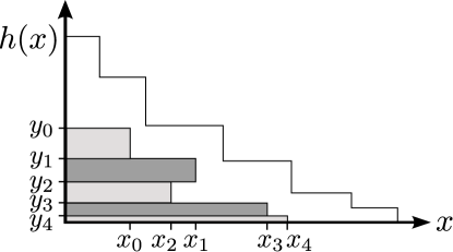
Figure 6: An illustration of the inequality $\int_{x=0}^{\infty}h(x)dx\geq\sum_{i\geq 0}x_{i}\left({y_{i}-y_{i+1}}\right)$.

Proof of Theorem 15: Let $Q:=\mathbb{E}\left[f(E,{\color[rgb]{0,0,0}{\Phi}})\right]$ be the maximum possible expected reward, where the expectation is taken w.r.t. ${\color[rgb]{0,0,0}{p\left({{\color[rgb]{0,0,0}{\phi}}}\right)}}$. Let $\pi$ be an $\alpha$-approximate greedy policy. Define $R_{i}:=Q-f_{\text{avg}}\left({\pi_{[{i}]}}\right)$ and define $P_{i}:=Q-f_{\text{avg}}\left({\pi_{[\leftarrow{i}]}}\right)$. Let $x_{i}:=\frac{P_{i}}{2s_{i}}$, let $y_{i}:=\frac{R_{i}}{2}$, and let $h(x):=Q-f_{\text{avg}}(\pi^{*}_{[{x}]})$. We claim $f_{\text{avg}}\left({\pi_{[\leftarrow{i}]}}\right)\leq f_{\text{avg}}\left({\pi_{[{i}]}}\right)$ and so $P_{i}\geq R_{i}$. This clearly holds if $\pi_{[\leftarrow{i}]}$ is the empty policy, and otherwise $\pi$ can always select an item that contributes zero marginal benefit, namely an item it has already played previously. Hence an $\alpha$-approximate greedy policy $\pi$ can never select items with negative expected marginal benefit, and so $f_{\text{avg}}\left({\pi_{[\leftarrow{i}]}}\right)\leq f_{\text{avg}}\left({\pi_{[{i}]}}\right)$. By Lemma 51, $f_{\text{avg}}\left({\pi^{*}_{[{x_{i}}]}}\right)\leq f_{\text{avg}}\left({\pi_{[\leftarrow{i}]}}\right)+x_{i}s_{i}$. Therefore

$$h(x_{i})\geq Q-f_{\text{avg}}(\pi_{[\leftarrow{i}]})-x_{i}\cdot s_{i}=P_{i}-\frac{P_{i}}{2}\geq\frac{R_{i}}{2}=y_{i}$$ (91)

For similar reasons that $f_{\text{avg}}\left({\pi_{[\leftarrow{i}]}}\right)\leq f_{\text{avg}}\left({\pi_{[{i}]}}\right)$, we have $f_{\text{avg}}\left({\pi_{[{i-1}]}}\right)\leq f_{\text{avg}}\left({\pi_{[{i}]}}\right)$, and so the sequence $\langle y_{1},y_{2},\ldots\rangle$ is non-increasing. The adaptive monotonicity and adaptive submodularity of $f$ imply that $h(x)$ is non-increasing. Informally, this is because otherwise, if $f_{\text{avg}}(\pi^{*}_{[{x}]})>f_{\text{avg}}(\pi^{*}_{[{x+1}]})$ for some $x$, then the optimal policy must be sacrificing immediate rewards at time $x$ in exchange for greater returns later, and it can be shown that if such a strategy is optimal, then adaptive submodularity cannot hold. Eq. (91) and the monotonicity of $h$ and $i\mapsto y_{i}$ imply that $\int_{x=0}^{\infty}h(x)dx\geq\sum_{i\geq 0}x_{i}\left({y_{i}-y_{i+1}}\right)$ (see Figure 6). The left hand side is a lower bound for $c_{\Sigma}\!\left({\pi^{*}}\right)$, and because $s_{i}=\alpha\left({R_{i}-R_{i+1}}\right)$ the right hand side simplifies to $\frac{1}{4\alpha}\sum_{i\geq 0}P_{i}=\frac{1}{4\alpha}c_{\Sigma}\!\left({\pi}\right)$, proving $c_{\Sigma}\!\left({\pi}\right)\leq 4\alpha\cdot c_{\Sigma}\!\left({\pi^{*}}\right)$. $\blacksquare$

15.6 A Symbol Table

$E$, $e\in E$	Ground set of items, and an individual item.
$O$, $o\in O$	States an item may be in, or outcomes of selecting an item, and an individual state/outcome.
${\color[rgb]{0,0,0}{\phi}}$	A realization, i.e., a function from items to states.
${\color[rgb]{0,0,0}{\psi}}$	A partial realization, typically encoding the current set of observations;
	each ${\color[rgb]{0,0,0}{\psi}}\subset E\times O$ is a partial mapping from items to states.
${\color[rgb]{0,0,0}{\Phi}},{\color[rgb]{0,0,0}{\Psi}}$	A random realization and a random partial realization, respectively.
$\sim$	The consistency relation: ${\color[rgb]{0,0,0}{\phi}}\sim{\color[rgb]{0,0,0}{\psi}}$ means ${\color[rgb]{0,0,0}{\psi}}(e)={\color[rgb]{0,0,0}{\phi}}(e)$ for all $e\in\operatorname{dom}({\color[rgb]{0,0,0}{\psi}})$.
${\color[rgb]{0,0,0}{p}}$	The probability distribution on realizations.
${\color[rgb]{0,0,0}{p}}({\color[rgb]{0,0,0}{\phi}}\mid{\color[rgb]{0,0,0}{\psi}})$	The conditional distribution on realizations: ${\color[rgb]{0,0,0}{p}}({\color[rgb]{0,0,0}{\phi}}\mid{\color[rgb]{0,0,0}{\psi}}):=\mathbb{P}\left[{\color[rgb]{0,0,0}{\Phi}}={\color[rgb]{0,0,0}{\phi}}\mid{\color[rgb]{0,0,0}{\Phi}}\sim{\color[rgb]{0,0,0}{\psi}}\right]$.
$\pi$	A policy, which maps partial realizations to items.
$E({\pi},{{\color[rgb]{0,0,0}{\phi}}})$	The set of all items selected by $\pi$ when run under realization ${\color[rgb]{0,0,0}{\phi}}$.
$\Delta\left({{e}\!\mid\!{{\color[rgb]{0,0,0}{\psi}}}}\right)$	The conditional expected marginal benefit of $e$ conditioned on ${\color[rgb]{0,0,0}{\psi}}$:
	$\Delta\left({{e}\!\mid\!{{\color[rgb]{0,0,0}{\psi}}}}\right):=\mathbb{E}\left[f(\operatorname{dom}({\color[rgb]{0,0,0}{\psi}})\cup\left\{e\right\},{\color[rgb]{0,0,0}{\Phi}})-f(\operatorname{dom}({\color[rgb]{0,0,0}{\psi}}),{\color[rgb]{0,0,0}{\Phi}})\ |\ {\color[rgb]{0,0,0}{\Phi}}\sim{\color[rgb]{0,0,0}{\psi}}\right]$.
$\Delta\left({{\pi}\!\mid\!{{\color[rgb]{0,0,0}{\psi}}}}\right)$	The conditional expected marginal benefit of policy $\pi$ conditioned on ${\color[rgb]{0,0,0}{\psi}}$:
	$\Delta\left({{\pi}\!\mid\!{{\color[rgb]{0,0,0}{\psi}}}}\right):=\mathbb{E}\left[f(\operatorname{dom}({\color[rgb]{0,0,0}{\psi}})\cup E({\pi},{{\color[rgb]{0,0,0}{\Phi}}}),{\color[rgb]{0,0,0}{\Phi}})-f(\operatorname{dom}({\color[rgb]{0,0,0}{\psi}}),{\color[rgb]{0,0,0}{\Phi}})\ |\ {\color[rgb]{0,0,0}{\Phi}}\sim{\color[rgb]{0,0,0}{\psi}}\right]$.
${{\color[rgb]{0,0,0}{\psi}}}\!\left[{e}/{o}\right]$	Shorthand for ${\color[rgb]{0,0,0}{\psi}}\cup\left\{(e,o)\right\}$.
$k$	Budget on the cost of selected item sets.
$\pi_{[{k}]}$	A truncated policy. See Definition 4 (unit costs) and Definition 32.
$\pi_{[\leftarrow{k}]}$	A strictly truncated policy. See Definition 30.
$\pi_{[{k}\to]}$	A laxly truncated policy. See Definition 31.
${\pi}@{\pi^{\prime}}$	Policies $\pi$ and $\pi^{\prime}$ concatenated together. See Definition 34.
$f$	An objective function, of type $f:2^{E}\times O^{E}\to\mathbb{R}_{\geq 0}$ unless stated otherwise.
$f_{\text{avg}}$	Average benefit: $f_{\text{avg}}(\pi):=\mathbb{E}\left[f(E({\pi},{{\color[rgb]{0,0,0}{\Phi}}}),{\color[rgb]{0,0,0}{\Phi}})\right]$.
$c$	Item costs $c:E\to\mathbb{N}$. Extended to sets via $c(S):=\sum_{e\in S}c(e)$.
${c_{\text{avg}}}$	Average cost of a policy: ${c_{\text{avg}}{(\pi)}}:=\mathbb{E}\left[c(E({\pi},{{\color[rgb]{0,0,0}{\Phi}}}))\right]$.
${c_{\text{wc}}}$	Worst-case cost of a policy: ${c_{\text{wc}}{(\pi)}}:=\max_{{\color[rgb]{0,0,0}{\phi}}}{c(E({\pi},{{\color[rgb]{0,0,0}{\phi}}}))}$.
$c_{\Sigma}$	Min-sum cost of a policy: $c_{\Sigma}\!\left({\pi}\right):=\sum_{t=0}^{\infty}\left({\mathbb{E}\left[f(E,{\color[rgb]{0,0,0}{\Phi}})\right]-f_{\text{avg}}(\pi_{[\leftarrow{t}]})}\right).$
$c\left({{\pi}\!\mid\!{{\color[rgb]{0,0,0}{\psi}}}}\right)$	Conditional average policy cost: $c\left({{\pi}\!\mid\!{{\color[rgb]{0,0,0}{\psi}}}}\right):=\mathbb{E}\left[c(E({\pi},{{\color[rgb]{0,0,0}{\Phi}}}))\mid{\color[rgb]{0,0,0}{\Phi}}\sim{\color[rgb]{0,0,0}{\psi}}\right]$.
$\alpha$	Approximation factor for greedy optimization in an $\alpha$-approximate greedy policy.
$Q$	Benefit quota. Often $Q=\mathbb{E}\left[f(E,{\color[rgb]{0,0,0}{\Phi}})\right]$.
$\eta$	Coverage gap: $\eta=\sup\left\{\eta^{\prime}:f(S,{\color[rgb]{0,0,0}{\phi}})>Q-\eta^{\prime}\text{ implies }f(S,{\color[rgb]{0,0,0}{\phi}})\geq Q\text{ for all }S,{\color[rgb]{0,0,0}{\phi}}\right\}$.
$\mathbf{1}_{P}$	The indicator for proposition $P$, which equals one if $P$ is true and zero if $P$ is false.

Table 2: Important symbols and notations used in this article

15.7 Proof of Approximation Hardness in the Absence of Adaptive Submodularity

We now provide the proof of Theorem 26 whose statement appears on page 26 in §12.

Proof of Theorem 26: We construct a hard instance based on the following intuition. We make the algorithm go “treasure hunting”. There is a set of $t$ locations $\left\{0,1,,\ldots,t-1\right\}$, there is a treasure at one of these locations, and the algorithm gets unit reward if it finds it, and zero reward otherwise. There are $m$ “maps,” each consisting of a cluster of $s$ bits, and each purporting to indicate where the treasure is, and each map is stored in a (weak) secret-sharing way, so that querying few bits of a map reveals nothing about where it says the treasure is. Moreover, all but one of the maps are fake, and there is a puzzle indicating which map is the correct one indicating the treasure’s location. Formally, a fake map is one which is probabilistically independent of the location of the treasure, conditioned on the puzzle.

Our instance will have three types of items, $E=E_{T}\uplus E_{M}\uplus E_{P}$, where $|E_{T}|=t$ encodes where the treasure is, $|E_{M}|=ms$ encodes the maps, and $|E_{P}|=n^{3}$ encodes the puzzle, where $m,t,s$ and $n$ are specified below. All outcomes are binary, so that $O=\{0,1\}$, and we identify items with bit indices. Accordingly we say that ${\color[rgb]{0,0,0}{\phi}}(e)$ is the value of bit $e$. For all $e\in E_{M}\cup E_{P}$, $\mathbb{P}\left[{\color[rgb]{0,0,0}{\Phi}}(e)=1\right]=.5$ independently. The conditional distribution of ${\color[rgb]{0,0,0}{\Phi}}(E_{T})$ given ${\color[rgb]{0,0,0}{\Phi}}(E_{M}\cup E_{P})$ will be deterministic as specified below. Our objective function $f$ is linear, and defined as follows:

$$f(A,{\color[rgb]{0,0,0}{\phi}})=|\{e\in A\cap E_{T}:{\color[rgb]{0,0,0}{\phi}}(e)=1\}|.$$

We now describe the puzzle, which is to compute $i(P):=(\operatorname{perm}(P)\mod p)\mod 2^{\ell}$ for a suitable random matrix $P$, and suitable prime $p$ and integer $\ell$, where $\operatorname{perm}(P)=\sum_{\sigma\in S_{n}}\prod_{i=1}^{n}P_{i\sigma(i)}$ is the permanent of $P$. We exploit Theorem $1.9$ of Feige and Lund (1997) in which they show that if there exist constants $\eta,\delta>0$ such that a randomized polynomial time algorithm can compute $(\operatorname{perm}(P)\mod p)\mod 2^{\ell}$ correctly with probability $2^{-\ell}(1+1/n^{\eta})$, where $P$ is drawn uniformly at random from $\left\{0,1,2,\ldots,p-1\right\}^{n\times n}$, $p$ is any prime superpolynomial in $n$, and $\ell\leq p\left({\frac{1}{2}-\delta}\right)$, then $\textrm{PH}=\textrm{AM}=\Sigma^{P}_{2}$. To encode the puzzle, we fix a prime $p\in[2^{n-2},2^{n-1}]$ and use the $n^{3}$ bits of ${\color[rgb]{0,0,0}{\phi}}(E_{P})$ to sample $P=P({\color[rgb]{0,0,0}{\phi}})$ (nearly) uniformly at random from $\left\{0,1,2,\ldots,p-1\right\}^{n\times n}$ as follows. For a matrix $P\in\mathbb{Z}^{n\times n}$, we let $\operatorname{rep}(P):=\sum_{ij}P_{ij}\cdot p^{(i-1)n+(j-1)}$ define a base $p$ representation of $P$. Note $\operatorname{rep}(\cdot)$ is one-to-one for $n\times n$ matrices with entries in $\mathbb{Z}_{p}$, so we can define its inverse $\operatorname{rep}^{-1}(\cdot)$. The encoding $P({\color[rgb]{0,0,0}{\phi}})$ interprets the bits ${\color[rgb]{0,0,0}{\phi}}(E_{P})$ as an integer $x$ in $[2^{n^{3}}]$, and computes $y=x\mod(p^{n^{2}})$. If $x\leq\left\lfloor 2^{n^{3}}/p^{n^{2}}\right\rfloor p^{n^{2}}$, then $P=\operatorname{rep}^{-1}(y)$. Otherwise, $P$ is the all zero matrix. This latter event occurs with probability at most $p^{n^{2}}/2^{n^{3}}\leq 2^{-n^{2}}$, and in this case we simply suppose the algorithm under consideration finds the treasure and so gets unit reward. This adds $2^{-n^{2}}$ to its expected reward. So let us assume from now on that $P$ is drawn uniformly at random.

Next we consider the maps. Partition $E_{M}=\biguplus_{i=1}^{m}M_{i}$ into $m$ maps $M_{i}$, each consisting of $s$ items. For each map $M_{i}$, partition its items into $s/\log_{2}t$ groups of $\log_{2}t$ bits each, so that the bits of each group encode a $\log_{2}t$ bit binary string. Let $v_{i}\in\left\{0,1,\ldots,t-1\right\}$ be the XOR of these $s/\log_{2}t$ binary strings, interpreted as an integer (using any fixed encoding). We say $M_{i}$ points to $v_{i}$ as the location of the treasure. A priori, each $v_{i}$ is uniformly distributed in $\{0,...,t-1\}$. For a particular realization of ${\color[rgb]{0,0,0}{\phi}}(E_{P}\cup E_{M})$, define $v({\color[rgb]{0,0,0}{\phi}}):=v_{i(P({\color[rgb]{0,0,0}{\phi}}))}$. We set $v({\color[rgb]{0,0,0}{\phi}})$ to be the location of the treasure under realization ${\color[rgb]{0,0,0}{\phi}}$, i.e., we label $E_{T}=\left\{e_{0},e_{1},\ldots,e_{t-1}\right\}$ and ensure ${\color[rgb]{0,0,0}{\phi}}(e_{j})=1$ if $j=v_{i(P({\color[rgb]{0,0,0}{\phi}}))}$, and ${\color[rgb]{0,0,0}{\phi}}(e)=0$ for all other $e\in E_{T}$. Note the random variable $v=v({\color[rgb]{0,0,0}{\phi}})$ is distributed uniformly at random in $\{0,1,\dots,t-1\}$. Note that this still holds if we condition on the realizations of any set of $s/\log_{2}t-1$ items in a map, because in this case there is still at least one group whose bits remain completely unobserved.

Now consider the optimal policy with a budget of $k=n^{3}+s+1$ items to pick. Clearly, its reward can be at most $1$. However, given a budget of $k$, a computationally unconstrained policy can exhaustively sample $E_{P}$, solve the puzzle (i.e., compute $i(P)$), read the correct map (i.e., exhaustively sample $M_{i(P)}$), decode the map (i.e., compute $v=v_{i(P)}$), and get the treasure (i.e., pick $e_{v}$) thereby obtaining a reward of one.

Now we give an upper bound on the expected reward $R$ of any randomized polynomial time algorithm $\mathcal{A}$ with a budget of $\beta k$ items, assuming $\Sigma^{P}_{2}\neq\textrm{PH}$. Fix a small constant $\gamma>0$, and set $s=n^{3}$ and $m=t=n^{1/\gamma}$. We suppose we give $\mathcal{A}$ the realizations ${\color[rgb]{0,0,0}{\phi}}(E_{M})$ for free. We also replace its budget of $\beta k$ items with a budget of $\beta k$ specifically for map items in $E_{M}$ and an additional budget of $\beta k$ specifically for the treasure locations in $E_{T}$. Obviously, this can only help it. As noted, if it selects less than $s/\log_{2}t$ bits from the map $M_{i(P)}$ indicated by $P$, the distribution over $v_{i(P)}$ conditioned on those realizations is still uniform. Of course, knowledge of $v_{i}$ for $i\neq i(P)$ is useless for getting reward. Hence $\mathcal{A}$ can try at most $\beta k\log_{2}(t)/s=o(\beta k)$ maps in an attempt to find $M_{i(P)}$. Note that if we have a randomized algorithm which given a random $P$ drawn from $\left\{0,1,2,\ldots,p-1\right\}^{n\times n}$ always outputs a set $S$ of integers of size $\alpha$ such that $\mathbb{P}\left[i(P)\in S\right]\geq q$, then we can use it to construct a randomized algorithm that, given $P$, outputs an integer $x$ such that $\mathbb{P}\left[i(P)=x\right]\geq q/\alpha$, simply by running the first algorithm and then selecting a random item of $S$. If $\mathcal{A}$ does not find $M_{i(P)}$, the distribution on the treasure’s location is uniform given its knowledge. Hence it’s budget of $\beta k$ treasure locations can only earn it expected reward at most $\beta k/t$. Armed with these observations and Theorem $1.9$ in the work of Feige and Lund (1997) and our complexity theoretic assumptions, we infer $\mathbb{E}\left[R\right]\leq o(\beta k)\cdot 2^{-\ell}(1+1/n^{\eta})+\beta k/t+2^{-n^{2}}$. Since $s=n^{3}$ and $m=t=n^{1/\gamma}$ and $\gamma=\Theta(1)$ and $\eta=1$ and $\ell=\log_{2}m$ and $k=n^{3}+s+1=2n^{3}+1$, we have

$$\mathbb{E}\left[R\right]\leq\frac{\beta k}{t}\left({1+o(1)}\right)=2\beta n^{3-1/\gamma}(1+o(1))\mbox{.}$$

Next note that $|E|=t+ms+n^{3}=n^{3+1/\gamma}(1+o(1))$. Straightforward algebra shows that in order to ensure $\mathbb{E}\left[R\right]=o(\beta/|E|^{1-\varepsilon})$, it suffices to choose $\gamma\leq\varepsilon/6$. Thus, under our complexity theoretic assumptions, any polynomial time randomized algorithm $\mathcal{A}$ with budget $\beta k$ achieves at most $o(\beta/|E|^{1-\varepsilon})$ of the value obtained by the optimal policy with budget $k$, so the approximation ratio is $\omega(|E|^{1-\varepsilon}/\beta)$. $\blacksquare$

References

- Alon et al. (2009) Noga Alon, Baruch Awerbuch, Yossi Azar, Niv Buchbinder, and Joseph Seffi Naor. The online set cover problem. SIAM Journal on Computing, 39:361–370, June 2009. ISSN 0097-5397. doi: 10.1137/060661946. URL http://portal.acm.org/citation.cfm?id=1654887.1654888.
- Arkin et al. (1993) Esther M. Arkin, Henk Meijer, Joseph S. B. Mitchell, David Rappaport, and Steven S. Skiena. Decision trees for geometric models. In Proceedings of Symposium on Computational Geometry, pages 369–378, New York, NY, USA, 1993. ACM. ISBN 0-89791-582-8. doi: http://doi.acm.org/10.1145/160985.161167.
- Asadpour et al. (2008) Arash Asadpour, Hamid Nazerzadeh, and Amin Saberi. Stochastic submodular maximization. In WINE ’08: Proceedings of the 4th International Workshop on Internet and Network Economics, pages 477–489, Berlin, Heidelberg, 2008. Springer-Verlag. ISBN 978-3-540-92184-4. doi: http://dx.doi.org/10.1007/978-3-540-92185-1˙53.
- Bellala and Scott (2010) G. Bellala and C. Scott. Modified group generalized binary search with near-optimal performance guarantees. Technical report, University of Michigan, 2010.
- Brochu et al. (2009) Eric Brochu, Mike Cora, and Nando de Freitas. A tutorial on Bayesian optimization of expensive cost functions, with application to active user modeling and hierarchical reinforcement learning. Technical Report TR-2009-23, Department of Computer Science, University of British Columbia, November 2009.
- Buchbinder and Naor (2009) Niv Buchbinder and Joseph (Seffi) Naor. The design of competitive online algorithms via a primal–dual approach. Foundations and Trends in Theoretical Computer Science, 3:93–263, February 2009. ISSN 1551-305X. doi: 10.1561/0400000024. URL http://portal.acm.org/citation.cfm?id=1576247.1576248.
- Chan and Farias (2009) Carri W. Chan and Vivek F. Farias. Stochastic depletion problems: Effective myopic policies for a class of dynamic optimization problems. Mathematics of Operations Research, 34(2):333–350, 2009. ISSN 0364-765X. doi: http://dx.doi.org/10.1287/moor.1080.0364.
- Cohn et al. (1996) David A. Cohn, Zoubin Gharamani, and Michael I. Jordan. Active learning with statistical models. Journal of Artificial Intelligence Research (JAIR), 4:129–145, 1996.
- Dantzig (1955) George B. Dantzig. Linear programming under uncertainty. Management Science, 1:197–206, 1955.
- Dasgupta (2004) Sanjoy Dasgupta. Analysis of a greedy active learning strategy. In NIPS: Advances in Neural Information Processing Systems 17, pages 337–344. MIT Press, 2004.
- Dean et al. (2005) B. Dean, M.X. Goemans, and J. Vondrák. Adaptivity and approximation for stochastic packing problems. In Proceedings of the 16th ACM-SIAM Symposium on Discrete Algorithms,, pages 395–404, 2005.
- Dean et al. (2008) B. Dean, M.X. Goemans, and J. Vondrák. Approximating the stochastic knapsack problem: The benefit of adaptivity. Mathematics of Operations Research, 33:945–964, 2008.
- Deshpande et al. (2004) A. Deshpande, C. Guestrin, S. Madden, J. Hellerstein, and W. Hong. Model-driven data acquisition in sensor networks. In Proceedings of the International Conference on Very Large Data Bases (VLDB), pages 588–599, 2004.
- Feige (1998) Uriel Feige. A threshold of ln n for approximating set cover. Journal of the ACM, 45(4):634 – 652, July 1998.
- Feige and Lund (1997) Uriel Feige and Carsten Lund. On the hardness of computing the permanent of random matrices. Computational Complexity, 6(2):101–132, 1997. ISSN 1016-3328. doi: http://dx.doi.org/10.1007/BF01262928.
- Feige et al. (2004) Uriel Feige, László Lovász, and Prasad Tetali. Approximating min sum set cover. Algorithmica, 40(4):219–234, 2004.
- Feldman and Vondrák (2012) Vitaly Feldman and Jan Vondrák. Private communication. 2012.
- Fujishige (2005) Satoru Fujishige. Submodular functions and optimization, volume 58. Annals of Discrete Mathematics, North Holland, Amsterdam, 2nd edition, 2005. ISBN 0-444-52086-4.
- Garey and Graham (1974) M. R. Garey and Ronald L. Graham. Performance bounds on the splitting algorithm for binary testing. Acta Informatica, 3:347–355, 1974.
- Gittins and Jones (1979) J. C. Gittins and D. M. Jones. A dynamic allocation index for the discounted multiarmed bandit problem. Biometrika, 66(3):561–565, December 1979.
- Goemans and Vondrák (2006) Michel X. Goemans and Jan Vondrák. Stochastic covering and adaptivity. In Proceedings of 7th International Latin American Symposium on Theoretical Informatics, pages 532–543, 2006.
- Golovin and Krause (2010) Daniel Golovin and Andreas Krause. Adaptive submodularity: A new approach to active learning and stochastic optimization. In 23rd Annual Conference on Learning Theory, pages 333–345, 2010.
- Golovin and Krause (2011a) Daniel Golovin and Andreas Krause. Adaptive submodularity: Theory and applications in active learning and stochastic optimization. Journal of Artificial Intelligence Research (JAIR), 42:427–486, 2011a.
- Golovin and Krause (2011b) Daniel Golovin and Andreas Krause. Adaptive submodular optimization under matroid constraints. CoRR, abs/1101.4450, 2011b.
- Golovin et al. (2008) Daniel Golovin, Anupam Gupta, Amit Kumar, and Kanat Tangwongsan. All-norms and all--norms approximation algorithms. In Ramesh Hariharan, Madhavan Mukund, and V Vinay, editors, IARCS Annual Conference on Foundations of Software Technology and Theoretical Computer Science (FSTTCS 2008), Dagstuhl, Germany, 2008. Schloss Dagstuhl - Leibniz-Zentrum fuer Informatik, Germany.
- Golovin et al. (2010) Daniel Golovin, Andreas Krause, and Debajyoti Ray. Near-optimal Bayesian active learning with noisy observations. In NIPS: Advances in Neural Information Processing Systems 23, pages 766–774. 2010.
- Golovin et al. (2011) Daniel Golovin, Andreas Krause, Beth Gardner, Sarah J. Converse, and Steve Morey. Dynamic resource allocation in conservation planning. In AAAI ’11: Proceedings of the Twenty–Fifth AAAI Conference on Artificial Intelligence, pages 1331–1336. AAAI Press, 2011.
- Goundan and Schulz (2007) Pranava R. Goundan and Andreas S. Schulz. Revisiting the greedy approach to submodular set function maximization. Technical report, Massachusetts Institute of Technology, 2007.
- Grünewälder et al. (2010) Steffen Grünewälder, Jean-Yves Audibert, Manfred Opper, and John Shawe-Taylor. Regret bounds for Gaussian process bandit problems. In Proceedings of the 13th International Conference on Artificial Intelligence and Statistics, 2010.
- Guha and Munagala (2009) Sudipto Guha and Kamesh Munagala. Multi-armed bandits with metric switching costs. In Proceedings of the International Colloquium on Automata, Languages and Programming (ICALP), 2009.
- Guha et al. (2009) Sudipto Guha, Kamesh Munagala, and Peng Shi. Approximation algorithms for restless bandit problems. Technical Report 0711.3861v5, arXiv, 2009.
- Guillory and Bilmes (2009) Andrew Guillory and Jeff Bilmes. Average-case active learning with costs. In The 20th International Conference on Algorithmic Learning Theory, University of Porto, Portugal, October 2009.
- Guillory and Bilmes (2010) Andrew Guillory and Jeff Bilmes. Interactive submodular set cover. In Proceedings of the International Conference on Machine Learning (ICML), number UWEETR-2010-0001, Haifa, Israel, 2010.
- Guillory and Bilmes (2011) Andrew Guillory and Jeff A. Bilmes. Simultaneous learning and covering with adversarial noise. In International Conference on Machine Learning (ICML), Bellevue, Washington, 2011.
- Gupta et al. (2005) Anupam Gupta, Martin Pál, R. Ravi, and Amitabh Sinha. What about Wednesday? Approximation algorithms for multistage stochastic optimization. In Proceedings of the 8th International Workshop on Approximation Algorithms for Combinatorial Optimization Problems (APPROX), 2005.
- Gupta et al. (2010) Anupam Gupta, Ravishankar Krishnaswamy, Viswanath Nagarajan, and R. Ravi. Approximation algorithms for optimal decision trees and adaptive TSP problems. In Proceedings of the International Colloquium on Automata, Languages and Programming (ICALP), volume 6198 of Lecture Notes in Computer Science, pages 690–701. Springer, 2010. ISBN 978-3-642-14164-5.
- Jones et al. (1998) Donald R. Jones, Matthias Schonlau, and William J. Welch. Efficient global optimization of expensive black-box functions. Journal of Global Optimization, 13:455–492, 1998.
- Kaplan et al. (2005) Haim Kaplan, Eyal Kushilevitz, and Yishay Mansour. Learning with attribute costs. In Proceedings of the ACM Symposium on Theory of Computing, pages 356–365, 2005.
- Kempe et al. (2003) David Kempe, Jon Kleinberg, and Éva Tardos. Maximizing the spread of influence through a social network. In KDD ’03: Proceedings of the ninth ACM SIGKDD international conference on Knowledge discovery and data mining, pages 137–146, New York, NY, USA, 2003. ACM. ISBN 1-58113-737-0. doi: http://doi.acm.org/10.1145/956750.956769.
- Kosaraju et al. (1999) S. Rao Kosaraju, Teresa M. Przytycka, and Ryan S. Borgstrom. On an optimal split tree problem. In Proceedings of the 6th International Workshop on Algorithms and Data Structures, pages 157–168, London, UK, 1999. Springer-Verlag. ISBN 3-540-66279-0.
- Krause and Guestrin (2005) A. Krause and C. Guestrin. Near-optimal nonmyopic value of information in graphical models. In Proceedings of Uncertainty in Artificial Intelligence (UAI), 2005.
- Krause and Guestrin (2007) Andreas Krause and Carlos Guestrin. Near-optimal observation selection using submodular functions. In Conference on Artificial Intelligence (AAAI) Nectar track, pages 1650–1654, 2007.
- Krause and Guestrin (2009a) Andreas Krause and Carlos Guestrin. Optimal value of information in graphical models. Journal of Artificial Intelligence Research (JAIR), 35:557–591, 2009a.
- Krause and Guestrin (2009b) Andreas Krause and Carlos Guestrin. Intelligent information gathering and submodular function optimization. Tutorial at the International Joint Conference in Artificial Intelligence, 2009b.
- Leskovec et al. (2007) Jure Leskovec, Andreas Krause, Carlos Guestrin, Christos Faloutsos, Jeanne VanBriesen, and Natalie Glance. Cost-effective outbreak detection in networks. In KDD ’07: Proceedings of the 13th ACM SIGKDD international conference on Knowledge discovery and data mining, pages 420–429, New York, NY, USA, 2007. ACM. ISBN 978-1-59593-609-7. doi: http://doi.acm.org/10.1145/1281192.1281239.
- Littman et al. (1998) M. Littman, J. Goldsmith, and M. Mundhenk. The computational complexity of probabilistic planning. Journal of Artificial Intelligence Research, 9:1–36, 1998.
- Liu et al. (2008) Zhen Liu, Srinivasan Parthasarathy, Anand Ranganathan, and Hao Yang. Near-optimal algorithms for shared filter evaluation in data stream systems. In SIGMOD ’08: Proceedings of the 2008 ACM SIGMOD international conference on Management of data, pages 133–146, New York, NY, USA, 2008. ACM. ISBN 978-1-60558-102-6. doi: http://doi.acm.org/10.1145/1376616.1376633.
- Lizotte et al. (2007) Daniel Lizotte, Tao Wang, Michael Bowling, and Dale Schuurmans. Automatic gait optimization with Gaussian process regression. In Proceedings of the Twentieth International Joint Conference on Artificial Intelligence (IJCAI), pages 944–949, 2007.
- Loveland (1985) Donald W. Loveland. Performance bounds for binary testing with arbitrary weights. Acta Informatica, 22(1):101–114, 1985. ISSN 0001-5903. doi: http://dx.doi.org/10.1007/BF00290148.
- McCallum and Nigam (1998) Andrew McCallum and Kamal Nigam. Employing EM and pool-based active learning for text classification. In Proceedings of the International Conference on Machine Learning (ICML), pages 350–358, 1998.
- Minoux (1978) Michel Minoux. Accelerated greedy algorithms for maximizing submodular set functions. In Proceedings of the 8th IFIP Conference on Optimization Techniques, pages 234–243. Springer, 1978.
- Munagala et al. (2005) Kamesh Munagala, Shivnath Babu, Rajeev Motwani, Jennifer Widom, and Eiter Thomas. The pipelined set cover problem. In Proceedings of the Intl. Conf. on Database Theory, pages 83–98, 2005.
- Nan and Saligrama (2017) F. Nan and V. Saligrama. Comments on the proof of adaptive stochastic set cover based on adaptive submodularity and its implications for the group identification problem in “group-based active query selection for rapid diagnosis in time-critical situations”. IEEE Transactions on Information Theory, 63(11):7612–7614, Nov 2017. ISSN 0018-9448. doi: 10.1109/TIT.2017.2749505.
- Nemhauser et al. (1978) George L. Nemhauser, Laurence A. Wolsey, and Marshall L. Fisher. An analysis of approximations for maximizing submodular set functions - I. Mathematical Programming, 14(1):265–294, 1978.
- Nowak (2009) Rob Nowak. Noisy generalized binary search. In NIPS: Advances in Neural Information Processing Systems 22, pages 1366–1374. 2009.
- Papadimitriou and Tsitsiklis (1987) C. H. Papadimitriou and J. N. Tsitsiklis. The complexity of Markov decision processses. Mathematics of Operations Research, 12(3):441–450, 1987.
- Pineau et al. (2006) Joelle Pineau, Geoff Gordon, and Sebastian Thrun. Anytime point-based approximations for large POMDPs. Journal of Artificial Intelligence Research (JAIR), 27:335–380, 2006.
- Raz and Safra (1997) Ran Raz and Shmuel Safra. A sub-constant error–probability low–degree test, and a sub–constant error-probability PCP characterization of NP. In STOC ’97: Proceedings of the twenty-ninth annual ACM Symposium on Theory of Computing, pages 475–484, New York, NY, USA, 1997. ACM. ISBN 0-89791-888-6. doi: http://doi.acm.org/10.1145/258533.258641.
- Ross et al. (2008) Stéphane Ross, Joelle Pineau, Sébastien Paquet, and Brahim Chaib-draa. Online planning algorithms for POMDPs. Journal of Artificial Intelligence Research, 32:663–704, July 2008. ISSN 1076-9757. URL http://portal.acm.org/citation.cfm?id=1622673.1622690.
- Schrijver (2003) Alexander Schrijver. Combinatorial optimization : polyhedra and efficiency. Volume B, Part IV, Chapters 39-49. Springer, 2003.
- Sebastiani and Wynn (2000) P. Sebastiani and H. P. Wynn. Maximum entropy sampling and optimal Bayesian experimental design. Journal of the Royal Statistical Society, Series B, 62(1):145–157, 2000.
- Smallwood and Sondik (1973) R.D. Smallwood and E.J. Sondik. The optimal control of partially observable Markov decision processes over a finite horizon. Operations Research, 21:1071–1088, 1973.
- Srinivas et al. (2010) Niranjan Srinivas, Andreas Krause, Sham Kakade, and Matthias Seeger. Gaussian process optimization in the bandit setting: No regret and experimental design. In Proceedings of the International Conference on Machine Learning (ICML), 2010.
- Streeter and Golovin (2007) Matthew Streeter and Daniel Golovin. An online algorithm for maximizing submodular functions. Technical Report CMU-CS-07-171, Carnegie Mellon University, 2007.
- Streeter and Golovin (2008) Matthew Streeter and Daniel Golovin. An online algorithm for maximizing submodular functions. In NIPS: Advances in Neural Information Processing Systems 21, pages 1577–1584, 2008.
- Wolsey (1982) Laurence A. Wolsey. An analysis of the greedy algorithm for the submodular set covering problem. Combinatorica, 2(4):385–393, 1982.