Experimental study of random close packed colloidal particles

Abstract

A collection of spherical particles can be packed tightly together into an amorphous packing known as “random close packing” (RCP). This structure is of interest as a model for the arrangement of molecules in simple liquids and glasses, as well as the arrangement of particles in sand piles. We use confocal microscopy to study the arrangement of colloidal particles in an experimentally realized RCP state. We image a large volume containing more than 450,000 particles with a resolution of each particle position to better than 0.02 particle diameters. While the arrangement of the particles satisfies multiple criteria for being random, we also observe a small fraction (less than 3%) of tiny crystallites (4 particles or fewer). These regions pack slightly better and are thus associated with locally higher densities. The structure factor of our sample at long length scales is non-zero, $S(0)=0.049\pm 0.008$, suggesting that there are long wavelength density fluctuations in our sample. These may be due to polydispersity or tiny crystallites. Our results suggest that experimentally realizable RCP systems may be different from simulated RCP systems, in particular, with the presence of these long wavelength density fluctuations.

I Introduction

Dense packings of hard spheres are an important starting point for the study of simple liquids, metallic glasses, colloids, biological systems, and granular matter Bernal ; Finney ; Scott ; Jodrey ; Tobochnik ; Lubachevsky ; Torquato2005 ; chaudhuri10 . Of particular interest is the densest possible packing that still possesses random structure, “random close packing” (RCP), which is important for physics and engineering. For example, the viscosity of dense particle suspensions diverges when the particles approach the RCP state Krieger . In a classic experiment, Bernal and Mason obtained the volume fraction of RCP $\phi_{RCP}\approx 0.637$. They compressed and shook a rubber balloon which was full of metal ball bearings for a sufficiently long time to achieve maximum density Bernal . Scott and Kilgour also reported $\phi_{RCP}\approx 0.637$ by pouring balls into a large vibrating container Scott . Their results were sensitive to the experimental method, for example both the frequency and amplitude of vibration. Likewise in computer simulations, the value of $\phi_{RCP}$ depends on the protocol. $\phi_{RCP}$ is between 0.642 and 0.648 with a rate dependent densification algorithm Jodrey , 0.68 with a Monte Carlo methods Tobochnik and 0.644 with Lubachevsky-Stillinger packing algorithm Lubachevsky ; Torquato2005 . All of these results are for monodisperse spheres, in other words, spheres with identical diameters.

The variety of results for $\phi_{RCP}$, in addition to being due to the method of preparing the RCP state, perhaps also comes from the poor definition of RCP Torquato2000 ; radin08 . The phrase “random close packing” is composed of two terms, “random” and “close packing,” which are inherently in conflict with each other. An ideal random state would have no correlation between particles, but the constraint that particles cannot overlap already diminishes the randomness of a physical packing. Furthermore, to get a close packing the most efficient method is to pack particles into a crystalline array, which is highly non-random Hales . For example, a random arrangement of spheres can be made denser if it partially includes dense crystalline regions, but then it is less random Davis ; Pouliquen . In 2000 Torquato and coworkers proposed “Maximum randomly jammed (MRJ)” state as a more tight definition of RCP. MRJ states are defined as the least locally ordered structures which are also jammed so that no particles can move Torquato2000 . A strictly jammed state should be incompressible and unshearable Torquato2003 , while other definitions of jammed states can involve external forces Cates or experimental time scales Liu ; the latter can involve questions of glassiness. Returning to strictly jammed states, one method of quantifying jamming is by considering the isothermal compressibility $K_{T}$, which is determined by the structure factor at wave number $q=0$, $K_{T}=1/\rho(\partial\rho/\partial p)=S(0)/\rho k_{B}T$ where $\rho$, $p$, $k_{B}$ and $T$ are density of the material, pressure, Boltzmann constant, and temperature, respectively. Thus, a strictly jammed state requires $K_{T}=S(0)=0$ since this state should be incompressible. Indeed, prior simulation works for the strict jammed state of hard spheres show $S(0)\approx 0$ to within numerical resolution Torquato2005 ; Torquato2003 ; Silbert . The observation $S(q\rightarrow 0)\rightarrow 0$ has been termed “hyperuniformity,” in that the density looks increasingly uniform when considered on longer length scales Torquato2005 .

The first physics study of the internal structure of a random closed packed system that we are aware of is the work of Smith, Foote, and Busang smith29 . In 1929, they studied the packing of shot and used acid to mark the contacts between spheres, reporting the contact numbers for 1,562 particles taken from the interior of a sample with 2,400 particles. In the 1960’s, Bernal first studied 500 particles taken from the interior of a sample with 5,000 particles Bernal , and later 1,000 particles bernal64 . In more recent times, 16,000 spheres were studied by Slotterback et al. who used an index-matching fluid and laser-sheet illumination to find the positions Losert . Aste et al. used x-ray tomography to study several different granular packings containing 90,000 particles in an interior region Aste . These experiments provide useful data for testing theories and studying the properties of RCP packings on large length scales.

In this article, we use a sedimented dense colloidal suspension as an experimental realization of a RCP material, in the loose sense of RCP rather than the strict sense of a MRJ state. We study the detailed structure of our sample with confocal microscopy, which can determine the three-dimensional positions of the particle centers to high accuracy. By carefully imaging overlapping regions, we observe a large volume containing over 450,000 particles. Our data set is available online epaps . The data are used to determine which features of our realistic RCP system are similar to the stricter ideal MRJ packing. The sample satisfies several criteria for randomness, for example, having only a tiny fraction of particles having even short-range order. However, in contrast to simulated MRJ packings, we find the isothermal compressibility is not zero, thus suggesting that in at least this particular experimental realization of a RCP system, there are differences with simulations.

It is important to note that our colloidal experiment differs in several particulars from both granular experiments (such as the early ones with ball bearings Bernal ; Scott ) and simulations. First, the particles are not all identical; they have a polydispersity of 5% in their diameters. Second, as the RCP state is formed by sedimentation, the particles have a chance to diffuse due to Brownian motion. In some situations this motion can help particles rearrange into crystalline packings, if the sample has a volume fraction in the range $0.49\leq\phi\leq 0.58$ Alder ; Pusey . While our experimental preparation method avoids full crystallization, it is plausible that the sample could be more ordered as a result of subtle rearrangements as particles sediment toward their final positions. However, conventionally such sedimented colloidal samples are thought of as RCP states. Our primary motivation is to use our sample to discern properties of the RCP state, and test the applicability of ideas derived from simulation.

II Method

II.1 Sample preparation

We use poly(methyl methacrylate) (PMMA) particles sterically stabilized with poly-12-hydroxystearic acid Antl . To visualize the particles, they are dyed with rhodamine 6G Dinsmore . The mean diameter $d$ of our particles is $d=2.53$ $\mu$m with an uncertainty 1%. Additionally the particles have a polydispersity of $\sim 5$%. According to prior simulations, the volume fraction for random close packing $\phi_{RCP}$ is between 0.64 and 0.66 for a 5% polydisperse system Farr ; schaertl94 ; hermes10 , which is almost same as $\phi_{RCP}$ for monodisperse spheres. References chaudhuri10 ; Torquato2000 ; hermes10 point out that the specific value often depends on the simulation details.

We use a fast laser scanning confocal microscope (VT-Eye, Visitech) which yields clear images deep inside our dense samples. Despite the high density, the colloidal particles can be easily discerned as shown in Fig. 1. We acquire three-dimensional (3D) scans of our sample yielding a $62.7\times 65.4\times 30$ $\mu$m³ observation volume for each image. As the sample is jammed, particles do not move and we can scan slowly to achieve very clean images: each 3D scan takes about 30 s. Within each 3D image, particles are identified within 0.03 $\mu$m in $x$ and $y$, and within 0.05 $\mu$m in $z$ Dinsmore ; Crocker96 .

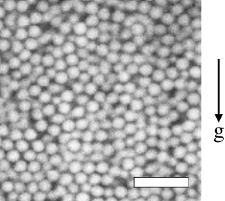
Figure 1: Confocal micrograph of the colloidal sediment in ($x$, $y$) plane. The image was taken 30 $\mu$m inside the sample. The scale bar represents 10 $\mu$m. The arrow indicates the direction of gravity during sedimentation.

The PMMA particles are initially suspended in a mixture of 85% cyclohexylbromide and 15% decalin by weight. This mixture closely matches both the density and refractive index of the particles Dinsmore . Then, to induce the particles to sediment, we add a small amount of decalin to slightly decrease the density of the dispersion fluid.

We can quantify the importance of sedimentation by computing the nondimensional Peclet number. This is the ratio of the time for a particle to diffuse its own radius $d/2$ to the time for it to fall a distance $d/2$. The diffusion time scale is $\tau_{D}=d^{2}/(8D)$, using the diffusion constant $D$, which for our particles and solvent is $D=0.1$ $\mu$m²/s. This gives us $\tau_{D}=6$ s. The sedimentation time scale is $\tau_{S}=d/(2v_{\rm sed})$. We observe the height of the sediment as a function of time in a macroscopic sample of dilute particles, and find $v_{\rm sed}=0.035$ $\mu$m/s, giving us $\tau_{S}=32$ s. Thus Pe $\approx 0.2$, suggesting that particles can diffuse long distances while they sediment; an alternate implication is that hydrodynamic interactions between particles due to sedimentation are perhaps less important than diffusion Segre . Prior to the start of sedimentation, the initial volume fraction is about 0.30 (in the stable liquid phase). We stir the particles by ultrasonic wave before sedimentation to avoid the Rayleigh-Taylor instability Wysocki . During sedimentation, the sample passes through the volume fraction range where crystals can be nucleated, approximately $0.51<\phi<0.60$ for our sample with 5% polydispersity pusey09 ; fasolo04 . We do not observe crystals in our final sample, and the most likely explanation is that sedimentation happens faster than nucleation, which is quite slow for polydisperse samples pusey09 ; auer01 ; schope07 . For samples with $Pe<0.1$, we do observe crystallization, although we have not carefully studied the critical $Pe$ for which crystallization is suppressed; see Ref. hermes10 for further discussion.

Given that diffusion is faster than sedimentation, the sample readily equilibrates, at least at low volume fractions as the sedimentation starts. Hence, we believe that our final state is well-defined and insensitive to the initial state. During sedimentation, the Stokes drag force acting on the particles is given by $F=3\pi\eta dv$, with viscosity $\eta=2.18$ mPa$\cdot$s and $v=v_{\rm sed}$. The buoyant weight of the particles is given by $W_{b}=\Delta\rho\pi d^{3}g/6$ with $g$ the acceleration due to gravity and $\Delta\rho$ being the density difference. Balancing the gravitational force with the drag force, we can estimate the density difference as $\Delta\rho=0.038$ g/cm³. For reference, the particle density is 1.2340 g/cm³. Balancing the gravitational energy $W_{b}h$ with the thermal energy $k_{B}T$ lets us determine the scale height $h=1.8$ $\mu$m (using $k_{B}$ as Boltzmann’s constant). The small scale height suggests that in the final sedimented state, there will be no density stratification except right at the interface between the dense sediment and the remaining solvent; that interface will have a thickness $O(h)$.

During the sedimentation process, it takes about 2 days for the sample to initially sediment to the bottom and form a glassy state. However, the sedimentation speed is slow at high $\phi$ Paddy ; Marconi . Thus, we wait 90 days to complete the sedimentation before we put the sample on the microscope. We also re-checked the sample 300 days after the initial sediment, and found the same results as a 90 day old sample.

We use the convention that the $y$ direction is the axis corresponding to gravity during the sedimentation process (see Fig. 1). The sample chamber is made from glass slides and coverslips, sealed with UV-curing epoxy (Norland), with the sample dimensions being $x=6$ mm, $y=20$ mm, and $z=0.14$ mm. When we measure the structure, we lay our sample on the microscope; that is, the optical $z$ axis is parallel to gravity and the microscope looks into the thinnest dimension of the sample chamber (for ease of viewing). In the highly concentrated sample, any subsequent gravity-induced particle rearrangements are much slower than our measuring time. In particular, we do not observe any particle flow in the sample, and the structure does not change at all during measurement. Near the flat coverslip of our sample chamber, particles layer against the wall Ken ; nugent07prl . To avoid influence of this, we take our 3D images at about 1 mm above the $y$ axis sample chamber bottom and at about 15 $\mu$m above the glass slide along the $z$ axis. Simulations show that wall effects decay fairly rapidly ($\sim 4$ diameters = 10 $\mu$m) Ken , and in our data we see no density fluctuations as a function of the distance $z$ away from the coverslip.

Of course, sedimentation with hydrodynamic interactions and Brownian motion is not a protocol followed in simulations of RCP states. The algorithm developed by Lubachevsky and Stillinger considers hard particles moving ballistically Lubachevsky . The particles start very small, and continue interacting as they gradually are swelled until the system jams. The method of O’Hern and co-workers is similar, starting with small particles that grow, but their particles are not infinitely hard, nor do they have velocities OHern . Rather, the simulation proceeds until the particles are maximally swelled but non-overlapping, thus giving the final hard-sphere state. Tobochnik and Chapin devised a similar algorithm which used Monte Carlo moves to eliminate overlaps Tobochnik . These “expand and eliminate the overlap” methods are similar to an earlier method due to Jodrey and Tory which slowly shrank spheres, sliding pairs of spheres linearly to minimize their overlap, until all spheres had no overlaps Jodrey . These methods all have the strength that the RCP state is generated isotropically, in contrast to our experiment where gravity sets a direction. (As discussed below, we do not see anything special about the direction of gravity in our data.) Our experimental method does have the feature that our spheres never overlap, in contrast to algorithms where overlaps are allowed at intermediate stages Jodrey ; OHern ; Tobochnik ; hermes10 , although it is not obvious that intermediate stage overlaps would cause substantially different results in the final state. In some ways our experimental protocol is similar to a method by Visscher and Bolsterli from 1972 visscher . Their algorithm dropped particles at random positions until the particles collided with the floor or a previous particle; the falling particle then rolls downhill until it reaches a locally stable position. In our experiment, all the particles fall simultaneously, and also their Brownian motion gives them the ability to find better packings than the Visscher and Bolsterli algorithm.

II.2 Connection of 3D images

To take a large ensemble, we scan a grid of 3D images with a small amount of overlap in $x$ and $y$. We compute particle positions from each image and then we connect one image to an adjacent overlapping image. Particles are considered as superimposed when $|\vec{r}_{ij}-\vec{r}_{lk}|<$ 0.2 $\mu$m where $\vec{r}_{ij}$ is the position of particle $i$ in image $j$ and $\vec{r}_{lk}$ is the position of particle $l$ in adjacent image $k$. To achieve this, we apply small displacement shifts $\Delta x$, $\Delta y$ and $\Delta z$ to one image, and look for the fraction $f$ of superimposed particles within the overlapped zones. Figure 2(a) shows $f$ in a ($\Delta x$, $\Delta y$) plane with the resolution of one pixel accuracy, and we find one spot where $f\sim 1$. The secondary ring around the central spot corresponds to the first peak of the pair correlation function, where some coincidences between particle positions are expected. While Fig. 2(a) shows $f$ in a two-dimensional plane, we calculate $f$ using shifts in the $z$ direction as well. We next apply sub-pixel displacement shifts around the spot in Fig. 2(a) to better resolve the peak. Finally, we calculate the sum of the squared distances between the positions of the overlapped particles within each region, and find the global choices of shift values that minimize the overall squared error, to provide the most accurate shift factors for the overlap. Using the shift factors, we then link up the particle positions in adjacent sections. The coincident particles are replaced by their average position. Figure 2(b) shows particle positions at $5<z<5.2$ $\mu$m after connecting 4 separate overlapping images. The particle positions are well-superimposed in the overlapping regions. Our sample chamber contains approximately 500,000,000 particles. Using the overlapping image method, we obtain a large 3D data set with size 492 $\mu$m $\times$ 513 $\mu$m $\times$ 28 $\mu$m, containing more than 500,000 particles. Due to artifacts when identifying particles near the image edges, we clip the data evenly from the boundaries and our final data set is $V=492$ $\mu$m $\times$ 513 $\mu$m $\times$ 23.5 $\mu$m, containing $N=453,136$ particles. This gives us $\phi_{RCP}=N(\pi d^{3}/6)/V=0.646\pm 0.020$, with the error bars due to the 1% uncertainty of the mean particle diameter. Our value is in agreement with simulations that considered polydispersity Farr ; schaertl94 .

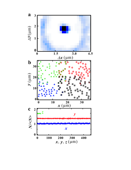
Figure 2: (color online) (a) The image plot of the fraction of successfully superimposed particles $f$ in a plane of ($\Delta x$, $\Delta y$). The dark central region corresponds to $f$ = 1, meaning that all possible particle overlaps are successful. (b) The circles, triangles, squares and crosses correspond to particle positions obtained from 4 separate 3D images. (c) The local number of particles observed $N$ normalized by the average, as a function of each axis after connecting the images. We add an offset to the data of $y$ and $z$ so they can be seen clearly.

We also examine the average number of particles $N$ observed as a function of $x$, $y$, and $z$. To do this as a function of $x$, we count the particles which are located between $x$ and $x+0.2$ $\mu$m for a sequence of $x$ values; a similar procedure is used for $N(y)$ and $N(z)$. The number of particles $N(x)$ as a function of $x$ is fairly flat, as are $N(y)$ and $N(z)$, as shown in Fig. 2(c). However, there are small residual oscillations in $x$ with the standard deviation of $N(x)/\langle N\rangle$ being 0.027 and a period of approximately 33 $\mu$m$\approx 13d$. This is an artifact of our connection algorithm, as we connect the images along $y$ direction first, then we connect them along the $x$ direction. If we change this order, we find $N(x)$ becomes flat and $N(y)$ undulates. To evaluate effects of this oscillation, we calculate the structure factor and the pair correlation function using both connection orders ($x$ first or $y$ first), and find almost identical results. Thus, we ignore these oscillations.

II.3 Detection of ordered particles

We use a rotationally invariant local bond order parameters $d_{6}$ to look for crystalline particles Steinhardt ; Wolde ; Gasser . The idea is to calculate for each particle a complex vector $q_{6m}(i)$, whose components $m$ depend on the orientation of the neighbors of particle $i$ relative to $i$. Each of the 13 components of the vector is given by:

$$q_{6m}(i)=\frac{1}{N_{b}}{\sum^{N_{b}}_{j=1}Y_{6m}(\hat{r}_{ij})},$$ (1)

where $N_{b}$ is the number of nearest neighbor particles for particle $i$, $\hat{r}_{ij}$ is the unit vector pointing from particle $i$ to its $j$th neighbor, and $Y_{lm}$ is a spherical harmonic function. The $q_{6m}$ parameters are the coefficients for the spherical harmonics in an expansion of the vector directions $\hat{r}_{ij}$, and thus capture a sense of the structure around particle $i$. The $l=6$ harmonics are used as it is known that on a local level, hexagonal symmetry is often present due to packing constraints Steinhardt ; Wolde . The neighbors of a particle are defined as those with centers separated by less than $1.4d$ (which is the location of the first minimum of the pair correlation function). These 13-dimensional complex vectors are then normalized to unity using

$$\hat{q}_{6m}(i)=\frac{q_{6m}(i)}{(\sum_{m}q_{6m}(i)\cdot q^{*}_{6m}(i))^{0.5}}.$$ (2)

Then, we compute $d_{6}$ as:

$$d_{6}(i,j)=\sum_{m=-6}^{6}q_{6m}(i)\cdot q^{*}_{6m}(j).$$ (3)

$d_{6}(i,j)$ is a normalized quantity correlating the local environments of neighboring $i$ and $j$ particles. $d_{6}(i,j)$ is a scalar and its range is $-1\leq d_{6}(i,j)\leq 1$; $d_{6}(i,j)=1$ would correspond to two particles who have identical local environments, at least identical in the sense captured by the $q_{6m}$ data. Two neighboring particles are termed “ordered neighbors” if $d_{6}(i,j)>0.5$. The number of ordered neighbors $N_{o}^{i}$ is decided for each particle. $N_{o}^{i}$ measures the amount of similarity of structure around neighboring particles. $N_{o}^{i}$=0 corresponds to random structure around particle $i$, while a large value of $N_{o}^{i}$ means that particle $i$ and its neighbor particles have similar surroundings. Following prior work, particles with $N_{o}^{i}\geq 8$ are classed as crystalline particles, and the other particles are liquid-like particles Wolde .

We also compute the $\hat{W}_{l}^{i}$ parameter to specify local structures: face centered cubic (fcc), icosahedral structure (icos), hexagonal close packed (hcp) and body centered cubic (bcc) Steinhardt . The $\hat{W}_{l}^{i}$ parameter is defined as

$$\bar{Q}^{i}_{lm} \equiv \langle Y_{lm}(\hat{r}_{ij})\rangle$$ (4)

$$W_{l}^{i} = \sum_{m_{1},m_{2},m_{3}}\left(\begin{array}[]{ccc}l&l&l\\ m_{1}&m_{2}&m_{3}\end{array}\right)\bar{Q}_{lm_{1}}^{i}\bar{Q}_{lm_{2}}^{i}\bar{Q}_{lm_{3}}^{i}$$ (7)

where $\langle\rangle$ corresponds to the average over neighboring particles $j$, $m_{1}+m_{2}+m_{3}=0$, and

$$\hat{W}_{l}^{i} \equiv W_{l}^{i}/\left(\sum^{l}_{m=-l}|\bar{Q}^{i}_{lm}|^{2}\right)^{3/2}.$$ (8)

The coefficients

$$\left(\begin{array}[]{ccc}l&l&l\\ m_{1}&m_{2}&m_{3}\end{array}\right)$$ (11)

are Wigner $3j$ symbols. Similar to the $q_{6m}$ parameters discussed above, the $\hat{W}_{l}$ parameters are able to capture a sense of the local ordering with $l$-fold symmetry, and have been used before to help classify local structure; see Ref. Steinhardt . The values of $\hat{W}_{l}^{i}$ for ideal structures are listed in Table 1 Steinhardt . These ideal structures are unrealistic for experimental data, so we generate 50,000 representations of each ordered structure and perturb their positions by 5 % of the particle diameter, to match the polydispersity of our experimental particle sizes. This gives us a distribution of $\hat{W}_{l}^{i}$ for each ordered structure (Table 2). Within our experimental data, we calculate $\hat{W}_{l}^{i}$ ($l$ = 4, 6, 8) for each particle. A particle is classed as a ordered particle when $\hat{W}_{4}$, $\hat{W}_{6}$ and $\hat{W}_{8}$ of a particle are simultaneously within the ranges of one structure shown in Table 2. Otherwise, particles are classed as random particles.

Table 1: The values of $\hat{W_{l}}$ ($l$ =4, 6, 8) for ideal structures of fcc, icosahedron, hcp and bcc Steinhardt . We add the notation of (i) for each ideal structure.

	$\hat{W}_{4}$	$\hat{W}_{6}$	$\hat{W}_{8}$
fcc(i)	-0.159316	-0.013161	0.058454
icos(i)		-0.169754
hcp(i)	0.134097	-0.012442	0.051259
bcc(i)	0.159317	0.013161	-0.058455

Table 2: The ranges of values of $\hat{W_{l}}$ ($l$ =4, 6, 8) for structures with 5% perturbations from ideal structures Steinhardt . We add the notation of (p) for the perturbed structures.

	$\hat{W}_{4}$	$\hat{W}_{6}$	$\hat{W}_{8}$
fcc(p)	-0.085 $\sim$ -0.169	-0.0109 $\sim$ -0.0193	-0.0180 $\sim$ 0.0640
icos(p)	-0.050 $\sim$ 0.200	-0.171 $\sim$ -0.162	-0.090 $\sim$ 0.090
hcp(p)	0.067 $\sim$ 0.138	-0.036 $\sim$ -0.004	0.000 $\sim$ 0.080
bcc(p)	0.152 $\sim$ 0.161	-0.015 $\sim$ 0.021	-0.072 $\sim$ 0.060

II.4 Calculating the structure factor

We compute the structure factor $S(\vec{q})$ via a direct Fourier transform of the particle position, $S(\vec{q})=N^{-1}|\sum^{N}_{i=1}\exp(i\vec{q}\cdot\vec{r}_{i})|^{2}$ where $\vec{r}_{i}$ is the particle position. $S(q)$ is the average of $S(\vec{q})$ over $q=\vec{q}$.

Our large images have two advantages for calculating the structure factor $S(q)$. The first is a high resolution with respect to $q$, as the resolution is given by $\delta q=2\pi/L$ where $L$ is the image size. Our sample size is 492 $\mu$m $\times$ 513 $\mu$m $\times$ 23.5 $\mu$m and this yields $\delta q=0.0128$ $\mu m^{-1}$. The second advantage of a large image is the reduction of boundary effects. Our experimental data set does not obey periodic boundary conditions, unlike most simulations. Thus, we need to use a window function to minimize the influence of the data cutting off at the boundaries, or we need to periodically replicate the data. Both these procedures increase $S(q)$ only near $q=0$, but it is precisely $S(q=0)$ that is of interest. Larger images allow us to go to smaller $q$ with less problems. We checked the Hann window, Hamming window, the Blackman window, and also using no window function. We find that $S(q)$ varies for $q<0.55$ $\mu m^{-1}$, corresponding to $qd/2\pi=0.2$. That is, our results for $q>0.55$ $\mu m^{-1}$ are independent of our choice of window functions. In what follows, we do not use a window function, and will focus on the results for small $q$ but considering only $q>0.55$ $\mu m^{-1}$.

III Results

III.1 Minimal local ordering

First, we investigate the randomness of our sample. We compute the fraction of ordered neighbors in the sediment of our colloidal suspension using the $d_{6}$ parameter described in Sec. II.3. Fig. 3(a) shows the probability of finding particles with a given number of ordered neighbors $N_{o}$. Following prior works, particles with $N_{o}^{i}\geq 8$ are classed as crystalline particles, and the other particles are liquid-like particles Wolde . We find the fraction of crystalline particles is below 0.03, and that these particles are well-dispersed throughout the sample, and shown in Fig. 3(b). At most, we see small crystallites composed of 3 or 4 crystalline particles which are nearest neighbors. Furthermore, the fraction of particles which $N_{o}$ is below 3 is over 0.8. It means that the coordinate particle arrangement of over 80% of particles are not similar to those of nearest neighbor particles. The effects on the structure by the spatial distribution of crystalline particles will be discussed below. We consider that our system is essentially randomly packed as the crystalline particles are a quite low fraction and well-dispersed.

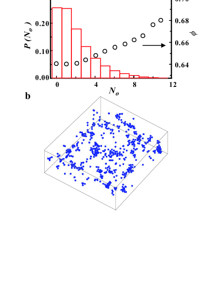
Figure 3: (color online). (a) The probability of the number of ordered neighbors $N_{o}$. When a particle has $N_{o}^{i}\geq 8$, it is classed as crystalline. The circles corresponds to local volume fraction calculated from Voronoi cell volume, averaged over all particles with $N_{o}$ having the given value. (b) The spatial distribution of crystalline particles in 3D image. This image is 115 $\mu$m $\times$ 115 $\mu$m $\times$ 23.5 $\mu$m. The other particles are not drawn, to better show the crystalline particles.

We also compute the fraction of specific local ordered structures: fcc, icosahedron structure (icos), hcp and bcc. The importance of those structures was emphasized over 50 years ago by Frank Frank ; for example, the icosahedral arrangement has a significantly lower energy than an hcp or fcc cluster for simple Lennard-Jones potentials. To specify local ordered structure, we compute $\hat{W}_{l}^{i}$ (l = 4, 6, 8) parameters for each particle Steinhardt (see Sec. II.3). We find that the fraction of particles that are fcc, icosahedron, hcp and bcc are 0.0020, 0.0001, 0.0066 and 0.0014, respectively. The sum of those fraction is $\sim$ 0.01 and this is consistent with the result of $N_{o}^{i}$ analysis. Again, this suggests that the sample is randomly packed. In addition, it is interesting that icosahedron is the least fraction we observe in our packed hard sphere-like particles, whereas icosahedral structure is most stable local structure for Lennard-Jones potentials Frank . This is consistent with many prior observations, and recent simulations suggest that icosahedral structures are indeed not as relevant for random close packed spheres as polytetrahedrons are more favored local structures vanmeel09 . We also find that the fraction of hcp ordering in our sample is higher than that of fcc.

III.2 Voronoi cell volume distribution

Next, we study the local volume fraction of the sediment at the particle length scale. We compute the Voronoi decomposition which is a unique partitioning of space. Each particle is within its own Voronoi polyhedron, and the Voronoi polyhedron is the region of space which is closer to the given particle than any other particle Preparata . We calculate a volume for each Voronoi cell except for those cells located on the boundaries, which have incorrectly defined volumes.

We compute the local volume fraction for each particle as $\phi_{i}=\pi\langle d\rangle^{3}/6V_{i}$ where $\phi_{i}$ and $V_{i}$ are the local volume fraction and Voronoi cell volume for particle $i$, respectively. We use the average diameter $d$ since we can not detect each particle diameter. The circles in Fig. 3(a) show the average local volume fraction as a function of $N_{o}$. We find that the local volume fraction is almost constant at $N_{o}\leq$ 2, but increases with larger $N_{o}$. This result means that few highly ordered particles have a higher local volume fraction than random particles. It is natural since ordered phase such as fcc crystal is the most packed phase and this tendency is suggested by previous reports Perera ; Luchnikov ; Eric2002 .

Next, we compute a distribution of Voronoi cell volume. Aste and coworkers proposed a universal function of the distribution of Voronoi cell volumes Aste , and the form is described as

$$P(V,k)=\frac{k^{k}}{(k-1)!}\frac{(V-V_{min})^{k-1}}{(\langle V\rangle-V_{min})^{k}}\exp\left(-k\frac{V-V_{min}}{\langle V\rangle-V_{min}}\right)$$ (12)

where $\langle V\rangle$ is the average of the Voronoi cell volumes. It is worth noting that the only adjustable parameter in Eq. 12 is $k$, other than $V_{min}$ which is constrained. $k$ is termed the “shape parameter” and corresponds the number of elementary cells composing the Voronoi cell Aste . For instance, the value of $k$ is 1 in an fcc crystal, while $k$ is close to the number of nearest neighbor particles (about 12 or 13) in random structure Aste . We choose $V_{min}=0.694d^{3}$, which is the smallest Voronoi cell that can be built in a packing of monodisperse spheres Aste . Figure 4(a) shows a distribution of the Voronoi cell volumes as a function of $(V-V_{min})/(\langle V\rangle-V_{min})$. The shape of the distribution is asymmetric and not Gaussian, that is, the distribution is narrow at small volumes and broad at large volumes. We fit the distribution of Voronoi cell volumes with Eq. 12 and obtain $k$ = 13.1 (the solid line in Fig. 4). The tail of the distribution is broader than the fitting line, perhaps due to the 5% polydispersity of our particles. The $k$ value was investigated in experiments using small glass beads ($\sim$ 250 $\mu$m) in water Aste , acrylic spheres with different preparation methods Aste and larger glass beads ($\sim$ 3 mm) in oil Losert . Those similar experiments found 11 $\leq k\leq$ 13 Aste and close to $k$ = 14.2 $\pm$ 0.6 Losert for random sphere packing. $k$ varies with each experiment since $k$ slightly depends on the polydispersity. Our experimentally observed value of $k$ = 13.1 is consistent with those prior experiments. This is further evidence that the arrangement of our sample is random. We note that a universality of $k$ value is proposed of the distribution of Voronoi cell volumes for random sphere packing, with the evidence coming from experimental with non Brownian particles Aste ; Losert . Our agreement with the prior work suggests that our close-packed sediment is not strongly different despite the Brownian motion that the particles have during sedimentation.

Within each Voronoi cell, we now consider the positions of particles relative to the Voronoi cell “center of mass.” We compute a vector $\vec{\Delta r}_{i}\equiv\vec{r}_{i}-\vec{g}_{i}$ where $\vec{r}_{i}$ is the position vector for particle $i$ and $\vec{g}_{i}$ is the position vector for the center of mass of the Voronoi cell which include particle $i$. Figure 4(b) shows the distribution of each axis component of $\vec{\Delta r}_{i}$. We find almost all particles are located at the centers of their Voronoi cells within the resolution of particle tracking ($\sim$ 0.05 $\mu$m), even along the direction of gravity.

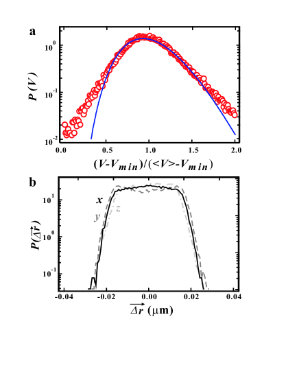
Figure 4: (color online) (a) Distribution of the Voronoi cell volumes plotted as a function of $(V-V_{min})/(\langle V\rangle-V_{min})$. The solid line is a fitting line with Eq. 12 using $k=13.1$. (b) Distribution of the position differences between the particle position and the center of mass of the Voronoi cell. Almost all particles are located at the center of mass of the Voronoi cell. The values on the horizontal axis only go from -0.04 to +0.04 $\mu$m, much less than the particle diameter $d=2.53$ $\mu$m.

III.3 Density fluctuations

We next check whether the sediment is in a “strictly jammed state” or not. As we mentioned above, $S(0)$ = 0 is required in strict jamming states since strict jamming states should be incompressible (equivalently, hyperuniform Torquato2005 ). To obtain $S(0)$ value, we directly calculate $S(\vec{q})$ from the particle positions. The inset in Fig. 5(a) shows a image plot of the structure factor in a plane of ($q_{x}$, $q_{y}$) where $q_{x}$ and $q_{y}$ are the $x$ and $y$ components of vector $q$. $S(\vec{q})$ is quite isotropic even though $y$ is the direction of gravity, again further implying our sediment is randomly packed. We average $S(\vec{q})$ over $q=|\vec{q}|$ and obtain $S(q)$, shown in Fig. 5(a). Figure 5(b) shows $S(q)$ near $q$=0 (circles). $S(q)$ increases near $q$ = 0 because of computational artifacts (see Sec. II.4); we find that $S(q)$ is reliable over $qd/2\pi\geq 0.2$, indicated by the vertical dashed line in the figure. We fit $S(q)$ with a linear function between $0.2\leq qd/2\pi\leq 0.5$ and obtain $S(0)=0.049\pm 0.008$ by extrapolation. $S(q)$ is also well fitted by a parabolic function between $0.2\leq qd/2\pi\leq 0.5$ and $S(0)$ is almost the same. Our data are insufficiently strong to determine if the linear fit or parabolic fit is more reasonable Torquato2005 . Our uncertainty (0.008) is determined by trying the different Fourier transform windowing functions, in combination with linear or parabolic fits: all possible combinations yield values within the range $S(0)=0.049\pm 0.008$, and thus we state with confidence that $S(0)\neq 0$. Donev, Stillinger and Torquato obtained $S(0)$ = 6.1 $\times$ $10^{-4}$ by numerical simulation with one million monodisperse particles Torquato2005 and our experimental value of $S(0)$ is about 100 times larger than simulation result, a significant difference well beyond the uncertainty of our data. This implies that our sample is much more compressive than the structure found by simulation.

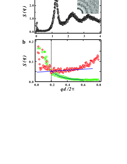
Figure 5: (color online) (a) The structure factor $S(q)$ as a function of wavenumber $q$. The inset is the quarter image of the structure factor in a plane of ($q_{x}$, $q_{y}$). (b) The expanded view of $S(q)$ (circles) and $S_{c}(q)$ (squares) near $q$ = 0. $S(q)$ increases near $q$ = 0 because of computational artifacts due to the finite size of our data set; the data are reliable for $qd/2\pi>0.2$, indicated by the vertical dashed line. The solid line is a fitting line with a linear function over the data with $0.2<qd/2\pi<0.5$. We obtain $S(0)$ = 0.049 by interpolating the fitting line to $q$ = 0. On the other hand, the structure factor for the crystalline particles $S_{c}(q)$ decreases with larger $q$ and it is well fitted by Ornstein-Zernike function (dashed line) over $0.2<qd/2\pi<0.6$.

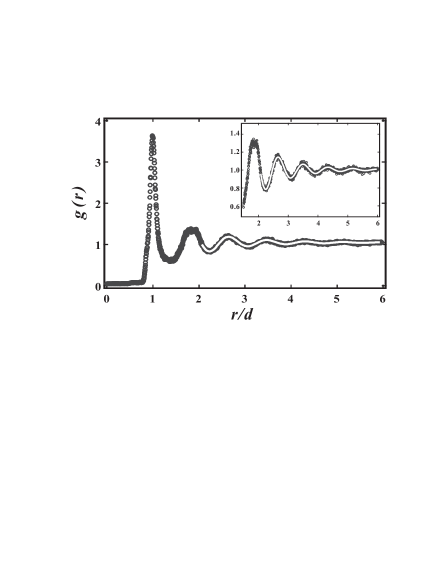
Figure 6: The pair correlation function $g(r)$ of the sediment. The inset is enlarged view at 2 $<r/d<$ 6. The solid line is a fitting line with Eq. 13 over $r/d>2$.

To support this result, we use a real space function: the pair correlation function $g(r)$ shown in Fig. 6. $g(r)$ at $r/d>$ 2 is well fitted by a exponentially damped oscillatory function Perry ; Torquato2002 described as:

$$g(r)\sim\frac{C}{r}\exp(-r/\xi)\cos[K_{0}(r-r_{0})]+1$$ (13)

where $C$, $\xi$ and $K_{0}$ correspond to an amplitude, a characteristic length of spatial correlation and the period of the oscillations, respectively. From the fitting, we obtain $C$ = 2.27 $\pm$ 0.08, $\xi=1.50d\pm 0.03d$ and $K_{0}=7.55/d\pm 0.01/d$. Again, we compare with the simulation of a strictly jammed state which yields $\xi=1.83d$ and $K_{0}=7.58/d$ Torquato2005 . Though $K_{0}$ is similar between experiment and simulation, the length scale $\xi$ from our experiment is shorter than that of simulation. The decay of $g(r)$ in an experiment is related to the broadness of each peak, that is, $g(r)$ decays quickly when peaks are slightly broad. Broad peaks mean that a distance between two particles are distributed. Hence, the rapid decay of $g(r)$ are also connected with the fluctuations in density, supporting the result $S(0)\neq 0$. Thus, we conclude that the arrangement in our experiment is not a strictly jammed state. It is important to note that uncertainty in particle positions will broaden the first peak of $g(r)$, but this does not strongly affect $g(r)$ for larger $r$ as those uncertainties do not accumulate over large distances. That is, the true separation between two particles has a distance $r_{ij}$ with an uncertainty of $\pm 0.06$ $\mu$m, which is somewhat significant when $r_{ij}$ is small and less important when $r_{ij}$ is large.

There are several possible explanations for this observed “softness.” One possibility is the polydispersity of colloidal size which is a crucial reality for experimental situations, and a difference with the simulations to which we are comparing our data. When particle sizes are slightly different, the minimum distance between two particles can be changed from $\langle d\rangle$ and then the first peak of $g(r)$ becomes slightly broad, consistent with Fig. 6. This small difference adds up over a long distance and then it may induce long wavelength fluctuations. In particular, the local fluctuations in composition (slightly more large particles or small particles) are coupled to the number fluctuations. A polydispersity of 5% such as we have in our experiment results in $S(q\rightarrow 0)=0.04\pm 0.01$ based on simulations ludovic , consistent with our data. Unfortunately, we cannot determine the individual particle sizes as the resolution of optical microscopy blurs particle images on the same scale as the variability of particle size. Furthermore, images of neighboring particles overlap, again due to the finite optical resolution. This makes determining individual particle size problematic, and prevents us from disentangling the influence of polydispersity from our data.

A second possibility is that our sample is not at random close packing due to friction effects between the particles, which is quite important for granular packings. It is known that granular packings are often looser than RCP, with volume fractions as low as $\phi\approx 0.58$, termed “random loose packing” Onoda . By vibrating the system, the packing fraction can be increased, perhaps coming close to RCP Bernal ; knight95 . In our experiment, particles move by Brownian motion, and this may let them find the RCP state. Furthermore, the particles are sterically stabilized to prevent them from sticking together. In general, friction is not a concept that is usually applied to colloidal particles. However, we cannot completely rule out the possibility of some possible occasional attractive interaction between our particles which might result in friction-like behavior, resulting in a slightly loose packing. Small amounts of static friction gave nonzero $S(0)$ values in simulations Silbert .

A third possibility is based on the $N_{o}$ dependence of the local volume fraction (Fig. 3(a)), that is, particles in more ordered local environments are packed better. The crystalline particles, which have high local volume fraction, are distributed throughout the sample (see Fig. 3(b)). To quantify the spatial distribution of the crystalline particles, we calculate a crystalline structure factor $S_{c}(q)$ as $S_{c}(\vec{q})={N}^{-1}|\sum^{N}_{i=1}W_{i}\exp(i\vec{q}\cdot\vec{r}_{i})|^{2}$ where $W_{i}$ = 1 when $i$ particle is classed as crystalline, otherwise $W_{i}$ = 0. $S_{c}(q)$ is the average of $S_{c}(\vec{q})$ over $q=\vec{q}$. The square symbols in Fig. 5(b) correspond to $S_{c}(q)$ and we find that $S_{c}(q)$ can be fitted with Ornstein-Zernike function [dashed line in Fig. 5(b)]. This fit gives us that the typical length scale between the crystalline particles is $12.8d\pm 1.8d$. Thus, the spatial distribution of crystalline particles can induce density fluctuations with long wavelength and it might be another reason for our observation that $S(0)\neq 0$. It is worth noting that the small but nonzero fraction of the crystallites (less than 3%) is crucial in this conjecture. It is possible that these tiny crystallites are due to Brownian motion during the sedimentation. We are unaware of any measurements of tiny crystallites in simulations of random close packing, although one recent study of a binary mixture of spheres used the same order parameter that we do and found the average number of ordered bonds (our $N_{o}$) was small Ken .

IV Conclusions

We use confocal microscopy to study both the local and long-range structure of a random close packed colloidal suspension. We find that the fraction of crystalline particles is at most 3%, and furthermore that almost no regions in the sample have icosohedral order (less than 0.01%). These observations suggest that the sample is randomly packed. This is further supported by the distribution of Voronoi volumes, which is well fit by a prediction based on a model of random packing.

We also compute the static structure factor $S(q)$ and find that $S(0)=0.05$, in contrast to simulations which found $S(0)=6\times 10^{-4}$ Torquato2005 . $S(0)$ is proportional to the isothermal compressibility, implying that the simulated states are essentially incompressible (to within numerical precision), while our experimental sample is compressible. This may be due to the presence of tiny crystalline regions in our sample, which are associated with slightly higher local density (and thus give rise to long wavelength density fluctuations). Alternatively, it may be due to the polydispersity of particle sizes in the experiment ($\sim 5$%). This softness ($S(0)\neq 0$) is crucial to how the sample would respond to an external force, for example, shear stress. The viscosity and elasticity of a sample are extremely sensitive to density near jamming point Olsson ; OHern . Near the jammed state, small fluctuations in density result in large fluctuations of viscosity and elasticity, which can lead to shear instability or cracking Furukawa . This suggests that real-world RCP materials may possess nontrivially different properties from idealized simulations. Our work points to polydispersity and sample preparation as the possible origin of these differences, both of which are worthy of further exploration in both simulation and experiment.

References

- (1) J. D. Bernal and J. Mason, Nature 188, 910 (1960).
- (2) J. L. Finney, Proc. R. Soc. London A 319, 479 (1970).
- (3) G. D. Scott and D. M. Kilgour, Br. J. Appl. Phys. 2, 863 (1969).
- (4) W. S. Jodrey and E. M. Tory, Phys. Rev. A 32, 2347 (1985).
- (5) J. Tobochnik and P. M. Chapin, J. Chem. Phys. 88, 5824 (1988).
- (6) B. D. Lubachevsky and F. H. Stillinger, J. Stat. Phys. 60, 561 (1990).
- (7) A. Donev, F. H. Stillinger and S. Torquato, Phys. Rev. Lett. 95, 090604 (2005).
- (8) P. Chaudhuri, L. Berthier, and S. Sastry, Phys. Rev. Lett. 104, 165701 (2010)
- (9) C. Radin, J. Stat. Phys. 131, 567 (2008).
- (10) I. M. Krieger, Adv. Colloid Interface Sci. 3, 111 (1972).
- (11) S. Torquato, T. M. Truskett and P. G. Debenedetti, Phys. Rev. Lett 84, 2064 (2000).
- (12) J. C. Hales, Ann. Math. 162, 1065 (2005).
- (13) K. E. Davis, W. B. Russel and W. J. Glantschnig, Science 245, 507 (1989).
- (14) O. Pouliquen, M. Nicolas and P. D. Weidman, Phys. Rev. Lett 79, 3640 (1997).
- (15) S. Torquato and F. H. Stillinger, Phys. Rev. E 68, 041113 (2003). 68, 069901 (2003).
- (16) M. E. Cates, J. P. Wittmer, J.-P. Bouchaud and P. Claudin, Phys. Rev. Lett. 81, 1841 (1998).
- (17) A. J. Liu and S. R. Nagel, Nature (London) 396, 6706 (1998).
- (18) L. E. Silbert and M. Silbert, Phys. Rev. E 80, 041304 (2009).
- (19) W. O. Smith, P. D. Foote, and P. F. Busang, Phys. Rev. 34, 1271 (1929).
- (20) J. D. Bernal, Proc. Roy. Soc. London. Ser. A 280, 299 (1964).
- (21) S. Slotterback, M. Toiya, L. Goff, J. F. Douglas and W. Losert, Phys. Rev. Lett. 101, 258001 (2008).
- (22) T. Aste, T. D. Matteo, M. Saadatfar, T. J. Senden, M. Schröter and H. L. Swinney, Euro. Phys. Lett. 79, 24003 (2007).
- (23) See supplementary material at [URL will be inserted by AIP] for a file of the particle coordinates.
- (24) B. J. Alder and T. E. Wainwright, J. Chem. Phys. 27, 1208 (1957).
- (25) P. N. Pusey and W. van Magen, Nature (London) 320, 340 (1986).
- (26) L. Antl, J. W. Goodwin, R. D. Hill, R. H. Ottewill, S. M. Owens, S. Papworth, and J. A. Waters, Colloid Surf. 17, 67 (1986).
- (27) A. D. Dinsmore, E. R. Weeks, V. Prasad, A. C. Levitt, and D. A. Weitz, Appl. Opt. 40, 4152 (2001).
- (28) R. S. Farr and R. D. Groot, J. Phys. Chem. 131, 244104 (2009).
- (29) W. Schaertl and H. Sillescu, J. Stat. Phys. 77, 1007 (1994).
- (30) M. Hermes and M. Dijkstra, Europhys. Lett. 89, 38005 (2010).
- (31) J. C. Crocker and D. G. Grier, J. Colloid Interface Sci. 179, 298 (1996).
- (32) P. N. Segrè , E. Herbolzheimer and P. M. Chaikin, Phys. Rev. Lett., 79, 2574 (1997).
- (33) A. Wysocki, C. P. Royall, R. G. Winkler, G. Gompper, H. Tanaka, A. van Blaaderen and H. Löwen, Soft Matter, 5, 1340 (2009).
- (34) P. N. Pusey, E. Zaccarelli, C. Valeriani, E. Sanz, W. C. K. Poon, and M. E. Cates, Phil. Trans. Roy. Soc. A 367, 4993 (2009).
- (35) M. Fasolo and P. Sollich, Phys. Rev. E 70, 041410 (2004).
- (36) S. Auer and D. Frenkel, Nature 413, 711 (2001).
- (37) H. J. Schope, G. Bryant, and W. van Megen, J. Chem. Phys. 127, 084505 (2007).
- (38) C. P. Royall, J. Dzubiella, M. Schmidt and A. van Blaaderen, Phys. Rev. Lett. 98, 188304 (2007).
- (39) U. Marini Bettolo Marconi and P. Tarazona, J. Chem. Phys. 110, 8032 (1999).
- (40) K. W. Desmond and E. R. Weeks, Phys. Rev. E 80, 051305 (2009).
- (41) C. R. Nugent, K. V. Edmond, H. N. Patel and E. R. Weeks, Phys. Rev. Lett. 99, 025702 (2007).
- (42) C. S. O’Hern, L. E. Silbert, A. J. Liu and S. R. Nagel Phys. Rev. E, 68, 011306 (2003).
- (43) W. M. Visscher and M. Bolsterli, Nature 239, 504 (1972).
- (44) P. J. Steinhardt, D. R. Nelson and M. Ronchetti, Phys. Rev. B 28, 784 (1983).
- (45) P. R. ten Wolde, M. J. Ruiz-Montero and D. Frenkel, J. Chem. Phys. 104, 9932 (1996).
- (46) U. Gasser, E. R. Weeks, A. Schofield, P. N. Pusey and D. A. Weitz, Science 292, 258 (2001).
- (47) F. C. Frank, Proc. R. Soc. London Ser. A 215, 43 (1952).
- (48) J. A. van Meel, D. Frenkel, and P. Charbonneau, Phys. Rev. E 79, 030201(R) (2009).
- (49) F. P. Preparata and M. I. Shamos, Computational Geometry (Springer-Verlag, New York, 1985).
- (50) D. N. Perera and P. Harrowell, J. Chem. Phys. 111, 5441 (1999).
- (51) V. A. Luchnikov, N. N. Medvedev, Yu. I. Naberukhin, V. N. Novikov, Phys. Rev. B 51, 15569 (1995).
- (52) E. R. Weeks and D. A. Weitz, Phys. Rev. Lett. 89, 095704 (2002).
- (53) P. Perry and G. J. Throop, J. Chem. Phys. 57, 1827 (1972).
- (54) S. Torquato and F. H. Stillinger, J. Phys. Chem. B 106, 8354 (2002); 106, 11406 (2002).
- (55) L. Berthier, personal communication.
- (56) G. Y. Onoda and E. G. Liniger, Phys. Rev. Lett. 64, 2727 (1990).
- (57) J. B. Knight, C. G. Fandrich, C. N. Lau, H. M. Jaeger, and S. R. Nagel, Phys. Rev. E 51, 3957 (1995).
- (58) P. Olsson and S. Teitel, Phys. Rev. Lett., 99, 178001 (2007).
- (59) A. Furukawa and H. Tanaka, Nat. Mat. 8, 601 (2009).