Weak Symplectic Fillings and Holomorphic Curves

Résumé.

English: We prove several results on weak symplectic fillings of contact $3$–manifolds, including: (1) Every weak filling of any planar contact manifold can be deformed to a blow up of a Stein filling. (2) Contact manifolds that have fully separating planar torsion are not weakly fillable—this gives many new examples of contact manifolds without Giroux torsion that have no weak fillings. (3) Weak fillability is preserved under splicing of contact manifolds along symplectic pre-Lagrangian tori—this gives many new examples of contact manifolds without Giroux torsion that are weakly but not strongly fillable.

We establish the obstructions to weak fillings via two parallel approaches using holomorphic curves. In the first approach, we generalize the original Gromov-Eliashberg “Bishop disk” argument to study the special case of Giroux torsion via a Bishop family of holomorphic annuli with boundary on an “anchored overtwisted annulus”. The second approach uses punctured holomorphic curves, and is based on the observation that every weak filling can be deformed in a collar neighborhood so as to induce a stable Hamiltonian structure on the boundary. This also makes it possible to apply the techniques of Symplectic Field Theory, which we demonstrate in a test case by showing that the distinction between weakly and strongly fillable translates into contact homology as the distinction between twisted and untwisted coefficients.

Français: On montre plusieurs résultats concernant les remplissages faibles de variétés de contact de dimension $3$, notamment : (1) Les remplissages faibles des variétés de contact planaires sont à déformation près des éclatements de remplissages de Stein. (2) Les variétés de contact ayant de la torsion planaire et satisfaisant une certaine condition homologique n’admettent pas de remplissages faibles – de cette manière on obtient des nouveaux exemples de variétés de contact qui ne sont pas faiblement remplissables. (3) La remplissabilité faible est préservée par l’opération de somme connexe le long de tores pré-Lagrangiens — ce qui nous donne beaucoup de nouveaux exemples de variétés de contact sans torsion de Giroux qui sont faiblement, mais pas fortement remplissables.

On établit une obstruction à la remplissabilité faible avec deux approches qui utilisent des courbes holomorphes. La première méthode se base sur l’argument original de Gromov-Eliashberg des «  disques de Bishop   ». On utilise une famille d’anneaux holomorphes s’appuyant sur un «  anneau vrillé ancré   » pour étudier le cas spécial de la torsion de Giroux. La deuxième méthode utilise des courbes holomorphes à pointes, et elle se base sur l’observation que dans un remplissage faible, la structure symplectique peut être déformée au voisinage du bord, en une structure Hamiltonienne stable. Cette observation permet aussi d’appliquer les méthodes à la théorie symplectique de champs, et on montre dans un cas simple que la distinction entre les remplissabilités faible et forte se traduit en homologie de contact par une distinction entre coefficients tordus et non tordus.

0. Introduction

The study of symplectic fillings via $J$–holomorphic curves goes back to the foundational result of Gromov [Gro85] and Eliashberg [Eli90a], which states that a closed contact $3$–manifold that is overtwisted cannot admit a weak symplectic filling. Let us recall some important definitions: in the following, we always assume that $(W,\omega)$ is a symplectic $4$–manifold, and $(M,\xi)$ is an oriented $3$–manifold with a positive and cooriented contact structure. Whenever a contact form for $\xi$ is mentioned, we assume it is compatible with the given coorientation.

Definition 1.

A contact $3$–manifold $(M,\xi)$ embedded in a symplectic $4$–manifold $(W,\omega)$ is called a contact hypersurface if there is a contact form $\alpha$ for $\xi$ such that $d\alpha={\left.{\omega}\right|_{TM}}$. In the case where $M=\partial W$ and its orientation matches the natural boundary orientation, we say that $(W,\omega)$ has contact type boundary $(M,\xi)$, and if $W$ is also compact, we call $(W,\omega)$ a strong symplectic filling of $(M,\xi)$.

Definition 2.

A contact $3$–manifold $(M,\xi)$ embedded in a symplectic $4$–manifold $(W,\omega)$ is called a weakly contact hypersurface if ${\left.{\omega}\right|_{\xi}}>0$, and in the special case where $M=\partial W$ with the natural boundary orientation, we say that $(W,\omega)$ has weakly contact boundary $(M,\xi)$. If $W$ is also compact, we call $(W,\omega)$ a weak symplectic filling of $(M,\xi)$.

It is easy to see that a strong filling is also a weak filling. In general, a strong filling can also be characterized by the existence in a neighborhood of $\partial W$ of a transverse, outward pointing Liouville vector field, i.e. a vector field $Y$ such that ${\mathcal{L}_{Y}}\omega=\omega$. The latter condition makes it possible to identify a neighborhood of $\partial W$ with a piece of the symplectization of $(M,\xi)$; in particular, one can then enlarge $(W,\omega)$ by symplectically attaching to $\partial W$ a cylindrical end.

The Gromov-Eliashberg result was proved using a so-called Bishop family of pseudoholomorphic disks: the idea was to show that in any weak filling $(W,\omega)$ whose boundary contains an overtwisted disk, a certain noncompact $1$–parameter family of $J$–holomorphic disks with boundary on $\partial W$ must exist, but yields a contradiction to Gromov compactness. In [Eli90a], Eliashberg also used these techniques to show that all weak fillings of the tight $3$–sphere are diffeomorphic to blow-ups of a ball. More recently, the Bishop family argument has been generalized by the first author [Nie06] to define the plastikstufe, the first known obstruction to symplectic filling in higher dimensions.

In the mean time, several finer obstructions to symplectic filling in dimension three have been discovered, including some which obstruct strong filling but not weak filling. Eliashberg [Eli96] used some of Gromov’s classification results for symplectic $4$–manifolds [Gro85] to show that on the $3$–torus, the standard contact structure is the only one that is strongly fillable, though Giroux had shown [Gir94] that it has infinitely many distinct weakly fillable contact structures. The first examples of tight contact structures without weak fillings were later constructed by Etnyre and Honda [EH02], using an obstruction due to Paolo Lisca [Lis99] based on Seiberg-Witten theory.

The simplest filling obstruction beyond overtwisted disks is the following. Define for each $n\in{\mathbb{N}}$ the following contact $3$–manifolds with boundary:

$$T_{n}:=\bigl{(}{\mathbb{T}}^{2}\times[0,n],\,\sin(2\pi z)\,d\varphi+\cos(2\pi z)\,d\vartheta\bigr{)}\;,$$

where $(\varphi,\vartheta)$ are the coordinates on ${\mathbb{T}}^{2}=\SS^{1}\times\SS^{1}$, and $z$ is the coordinate on $[0,n]$. We will refer to $T_{n}$ as a Giroux torsion domain.

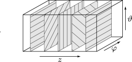
Figure 1. The region between the grey planes on either side represents half a Giroux torsion domain. The grey planes are pre-Lagrangian tori with their characteristic foliations, which show the contact structure turning along the $z$–axis as we move from left to right. Domains with higher Giroux torsion can be constructed by gluing together several half-torsion domains.

Definition 3.

Let $(M,\xi)$ be a $3$–dimensional contact manifold. The Giroux torsion $\operatorname{Tor}(M,\xi)\in{\mathbb{Z}}\cup\{\infty\}$ is the largest number $n\geq 0$ for which we can find a contact embedding of the Giroux torsion domain $T_{n}\hookrightarrow M$. If this is true for arbitrarily large $n$, then we define $\operatorname{Tor}(M,\xi)=\infty$.

Remark.

Due to the classification result of Eliashberg [Eli89], overtwisted contact manifolds have infinite Giroux torsion, and moreover, one can assume in this case that the torsion domain $T_{n}\subset M$ separates $M$. It is not known whether a contact manifold with infinite Giroux torsion must be overtwisted in general.

The present paper was motivated partly by the following fairly recent result.

Theorem (Gay [Gay06] and Ghiggini-Honda [GH08]).

A closed contact $3$–manifold $(M,\xi)$ with positive Giroux torsion does not have a strong symplectic filling. Moreover, if it contains a Giroux torsion domain $T_{n}$ that splits $M$ into separate path components, then $(M,\xi)$ does not even admit a weak filling.

The first part of this statement was proved originally by David Gay with a gauge theoretic argument, and the refinement for the separating case follows from a computation of the Ozsváth-Szabó contact invariant due to Paolo Ghiggini and Ko Honda. Observe that due to the remark above on overtwistedness and Giroux torsion, the result implies the Eliashberg-Gromov theorem.

As this brief sampling of history indicates, holomorphic curves have not been one of the favorite tools for defining filling obstructions in recent years. One might argue that this is unfortunate, because holomorphic curve arguments have a tendency to seem more geometrically natural and intuitive than those involving the substantial machinery of Seiberg-Witten theory or Heegaard Floer homology—and in higher dimensions, of course, they are still the only tool available. A recent exception was the paper [Wen10c], where the second author used families of holomorphic cylinders to provide a new proof of Gay’s result on Giroux torsion and strong fillings. By similar methods, the second author has recently defined a more general obstruction to strong fillings [Wen10b], called planar torsion, which provides many new examples of contact manifolds $(M,\xi)$ with $\operatorname{Tor}(M,\xi)=0$ that are nevertheless not strongly fillable. The reason these results apply primarily to strong fillings is that they depend on moduli spaces of punctured holomorphic curves, which live naturally in the noncompact symplectic manifold obtained by attaching a cylindrical end to a strong filling. By contrast, the Eliashberg-Gromov argument works also for weak fillings because it uses compact holomorphic curves with boundary, which live naturally in a compact almost complex manifold with boundary that is pseudoconvex, but not necessarily convex in the symplectic sense. The Bishop family argument however has never been extended for any compact holomorphic curves more general than disks, because these tend to live in moduli spaces of nonpositive virtual dimension.

In this paper, we will demonstrate that both approaches, via compact holomorphic curves with boundary as well as punctured holomorphic curves, can be used to prove much more general results involving weak symplectic fillings. As an illustrative example of the compact approach, we shall begin in §1 by presenting a new proof of the above result on Giroux torsion, as a consequence of the following.

Theorem 1.

Let $(M,\xi)$ be a closed $3$–dimensional contact manifold embedded into a closed symplectic $4$–manifold $(W,\omega)$ as a weakly contact hypersurface. If $(M,\xi)$ contains a Giroux torsion domain $T_{n}\subset M$, then the restriction of the symplectic form $\omega$ to $T_{n}$ cannot be exact.

By a theorem of Eliashberg [Eli04] and Etnyre [Etn04a], every weak filling can be capped to produce a closed symplectic $4$–manifold. The above statement thus implies a criterion for $(M,\xi)$ to be not weakly fillable—our proof will in fact demonstrate this directly, without any need for the capping result. We will use the fact that every Giroux torsion domain contains an object that we call an anchored overtwisted annulus, which we will show serves as a filling obstruction analogous to an overtwisted disk. Note that for a torsion domain $T_{n}\subset M$, the condition that $\omega$ is exact on $T_{n}$ is equivalent to the vanishing of the integral

$$\int_{{\mathbb{T}}^{2}\times\{c\}}\omega$$

on any slice $T^{2}\times\{c\}\subset T_{n}$. For a strong filling this is always satisfied since $\omega$ is exact on the boundary, and it is also always satisfied if $T_{n}$ separates $M$.

The proof of Theorem 1 is of some interest in itself for being comparatively low-tech, which is to say that it relies only on technology that was already available as of 1985. As such, it demonstrates new potential for well established techniques, in particular the Gromov-Eliashberg Bishop family argument, which we shall generalize by considering a “Bishop family of holomorphic annuli” with boundaries lying on a $1$–parameter family of so-called half-twisted annuli. Unlike overtwisted disks, a single overtwisted annulus does not suffice to prove anything: the boundaries of the Bishop annuli must be allowed to vary in a nontrivial family, called an anchor, so as to produce a moduli space with positive dimension. One consequence of this extra degree of freedom is that the required energy bounds are no longer automatic, but in fact are only satisfied when $\omega$ satisfies an extra cohomological condition. This is one way to understand the geometric reason why Giroux torsion always obstructs strong fillings, but only obstructs weak fillings in the presence of extra topological conditions. This method also provides some hope of being generalizable to higher dimensions, where the known examples of filling obstructions are still very few.

In §2, we will initiate the study of weak fillings via punctured holomorphic curves in order to obtain more general results. The linchpin of this approach is Theorem 2.9 in §2.2, which says essentially that any weak filling can be deformed so that its boundary carries a stable Hamiltonian structure. This is almost as good as a strong filling, as one can then symplectically attach a cylindrical end—but extra cohomological conditions are usually needed in order to do this without losing the ability to construct nice holomorphic curves in the cylindrical end. It turns out that the required conditions are always satisfied for planar contact manifolds, and we obtain the following surprising generalization of a result proved for strong fillings in [Wen10c].

Theorem 2.

If $(M,\xi)$ is a planar contact $3$–manifold, then every weak filling of $(W,\omega)$ is symplectically deformation equivalent to a blow up of a Stein filling of $(M,\xi)$.

Corollary 1.

If $(M,\xi)$ is weakly fillable but not Stein fillable, then it is not planar.

Corollary 2.

Given any planar open book supporting a contact manifold $(M,\xi)$, the manifold is weakly fillable if and only if the monodromy of the open book can be factored into a product of positive Dehn twists.

The second corollary follows easily from the result proved in [Wen10c], that every planar open book on a strongly fillable contact manifold can be extended to a Lefschetz fibration of the filling over the disk. This fact was used in recent work of Olga Plamenevskaya and Jeremy Van Horn-Morris [PVHM10] to find new examples of planar contact manifolds that have either unique fillings or no fillings at all. Theorem 2 in fact reduces the classification question for weak fillings of planar contact manifolds to the classification of Stein fillings, and as shown in [Wen] using the results in [Wen10c], the latter reduces to an essentially combinatorial question involving factorizations of monodromy maps into products of positive Dehn twists. Note that most previous classification results for weak fillings (e.g. [Eli90a, Lis08, PVHM10]) have applied to rational homology spheres, as it can be shown homologically in such settings that weak fillings are always deformable to strong ones. Theorem 2 makes no such assumption about the topology of $M$.

Remark.

It is easy to see that nothing like Theorem 2 holds for non-planar contact manifolds in general. There are of course many examples of weakly but not strongly fillable contact manifolds; still more will appear in the results stated below. There are also Stein fillable contact manifolds with weak fillings that cannot be deformed into blown up Stein fillings: for instance, Giroux shows in [Gir94] that the standard contact $3$–torus $({\mathbb{T}}^{3},\xi_{1})$ admits weak fillings diffeomorphic to $\Sigma\times{\mathbb{T}}^{2}$ for any compact oriented surface $\Sigma$ with connected boundary. As shown in [Wen10c] however, $({\mathbb{T}}^{3},\xi_{1})$ has only one Stein filling, diffeomorphic to ${\mathbb{D}}\times{\mathbb{T}}^{2}$, and if $\Sigma\neq{\mathbb{D}}$ then $\Sigma\times{\mathbb{T}}^{2}$ is not homeomorphic to any blow-up of ${\mathbb{D}}\times{\mathbb{T}}^{2}$, since $\pi_{2}(\Sigma\times{\mathbb{T}}^{2})=0$.

Using similar methods, §2 will also generalize Theorem 1 to establish a new obstruction to weak symplectic fillings in dimension three. We will recall in §2.3 the definition of a planar torsion domain, which is a generalization of a Giroux torsion domain that furnishes an obstruction to strong filling by a result in [Wen10b]. The same will not be true for weak fillings, but becomes true after imposing an extra homological condition: for any closed $2$–form $\Omega$ on $M$, one says that $M$ has $\Omega$–separating planar torsion if

$$\int_{L}\Omega=0$$

for every torus $L$ in a certain special set of disjoint tori in the torsion domain.

Theorem 3.

Suppose $(M,\xi)$ is a closed contact $3$–manifold with $\Omega$–separating planar torsion for some closed $2$–form $\Omega$ on $M$. Then $(M,\xi)$ admits no weakly contact type embedding into a closed symplectic $4$–manifold $(W,\omega)$ with ${\left.{\omega}\right|_{TM}}$ cohomologous to $\Omega$. In particular, $(M,\xi)$ has no weak filling $(W,\omega)$ with $[{\left.{\omega}\right|_{TM}}]=[\Omega]$.

As is shown in [Wen10b], any Giroux torsion domain embedded in a closed contact manifold has a neighborhood that contains a planar torsion domain, thus Theorem 3 implies another proof of Theorem 1. If each of the relevant tori $L\subset M$ separates $M$, then $\int_{L}\Omega=0$ for all $\Omega$ and we say that $(M,\xi)$ has fully separating planar torsion.

Corollary 3.

If $(M,\xi)$ is a closed contact $3$–manifold with fully separating planar torsion, then it admits no weakly contact type embedding into any closed symplectic $4$–manifold. In particular, $(M,\xi)$ is not weakly fillable.

Remark.

The statement about non-fillability in Corollary 3 also follows from a recent computation of the twisted ECH contact invariant that has been carried out in parallel work of the second author [Wen10b]. The proof via ECH is however extremely indirect, as according to the present state of technology it requires the isomorphism established by Taubes [Tau] from ECH to monopole Floer homology, together with results of Kronheimer and Mrowka [KM97] that relate the monopole invariants to weak fillings. Our proof on the other hand will require no technology other than holomorphic curves.

We now show that there are many contact manifolds without Giroux torsion that satisfy the above hypotheses. Consider a closed oriented surface

$$\Sigma=\Sigma_{+}\cup_{\Gamma}\Sigma_{-}$$

obtained as the union of two (not necessarily connected) surfaces $\Sigma_{\pm}$ with boundary along a multicurve $\Gamma\neq\emptyset$. By results of Lutz [Lut77], the $3$–manifold $\SS^{1}\times\Sigma$ admits a unique (up to isotopy) $\SS^{1}$–invariant contact structure $\xi_{\Gamma}$ such that the surfaces $\{*\}\times\Sigma$ are all convex and have $\Gamma$ as the dividing set. If $\Gamma$ has no component that bounds a disk, then the manifold $(\SS^{1}\times\Sigma,\xi_{\Gamma})$ is tight [Gir01, Proposition 4.1], and if $\Gamma$ also has no two connected components that are isotopic in $\Sigma$, then it follows from arguments due to Giroux (see [Mas09]) that $(\SS^{1}\times\Sigma,\xi_{\Gamma})$ does not even have Giroux torsion. But as we will review in §2.3, it is easy to construct examples that satisfy these conditions and have planar torsion.

Corollary 4.

For the $\SS^{1}$–invariant contact manifold $(\SS^{1}\times\Sigma,\xi_{\Gamma})$ described above, suppose the following conditions are satisfied (see Figure 2):

1. $\Gamma$ has no contractible components and no pair of components that are isotopic in $\Sigma$.

2. $\Sigma_{+}$ contains a connected component $\Sigma_{P}\subset\Sigma_{+}$ of genus zero, whose boundary components each separate $\Sigma$.

Then $(\SS^{1}\times\Sigma,\xi_{\Gamma})$ has no Giroux torsion and is not weakly fillable.

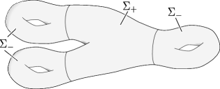
Figure 2. An example of a surface $\Sigma$ and multicurve $\Gamma\subset\Sigma$ satisfying the conditions of Corollary 4.

The example of the tight $3$–tori shows that the homological condition in the Giroux torsion case cannot be relaxed, and indeed, the first historical examples of weakly but not strongly fillable contact structures can in hindsight be understood via the distinction between separating and non-separating Giroux torsion. In §3, we will introduce a new symplectic handle attachment technique that produces much more general examples of weak fillings:

Theorem 4.

Suppose $(W,\omega)$ is a (not necessarily connected) weak filling of a contact $3$–manifold $(M,\xi)$, and $T\subset M$ is an embedded oriented torus which is pre-Lagrangian in $(M,\xi)$ and symplectic in $(W,\omega)$. Then:

1. $(W,\omega)$ is also a weak filling of every contact manifold obtained from $(M,\xi)$ by performing finitely many Lutz twists along $T$.

2. If $T^{\prime}\subset M$ is another torus satisfying the stated conditions, disjoint from $T$, such that $\int_{T}\omega=\int_{T^{\prime}}\omega$, then the contact manifold obtained from $(M,\xi)$ by splicing along $T$ and $T^{\prime}$ is also weakly fillable.

See §3 for precise definitions of the Lutz twist and splicing operations, as well as more precise versions of Theorem 4. We will use the theorem to explicitly construct new examples of contact manifolds that are weakly but not strongly fillable, including some that have planar torsion but no Giroux torsion. Let

$$\Sigma=\Sigma_{+}\cup_{\Gamma}\Sigma_{-}$$

be a surface divided by a multicurve $\Gamma$ into two parts as described above. The principal circle bundles $P_{\Sigma,e}$ over $\Sigma$ are distinguished by their Euler number $e=e(P)\in{\mathbb{Z}}$ which can be easily determined by removing a solid torus around a fiber of $P_{\Sigma,e}$, choosing a section outside this neighborhood, and computing the intersection number of the section with a meridian on the torus. The Euler number thus measures how far the bundle is from being trivial. Lutz [Lut77] also showed that every nontrivial $\SS^{1}$–principal bundle $P_{\Sigma,e}$ with Euler number $e$ over $\Sigma$ admits a unique (up to isotopy) $\SS^{1}$–invariant contact structure $\xi_{\Gamma,e}$ that is tangent to fibers over the multicurve $\Gamma$ and is everywhere else transverse. For simplicity, we will continue to write $\xi_{\Gamma}$ for the corresponding contact structure $\xi_{\Gamma,0}$ on the trivial bundle $P_{\Sigma,0}=\SS^{1}\times\Sigma$.

Theorem 5.

Suppose $\bigl{(}P_{\Sigma,e},\xi_{\Gamma,e}\bigr{)}$ is the $\SS^{1}$–invariant contact manifold described above, for some multicurve $\Gamma\subset\Sigma$ whose connected components are all non-separating. Then $\bigl{(}P_{\Sigma,e},\xi_{\Gamma,e}\bigr{)}$ is weakly fillable.

Corollary 5.

There exist contact $3$–manifolds without Giroux torsion that are weakly but not strongly fillable. In particular, this is true for the $\SS^{1}$–invariant contact manifold $(\SS^{1}\times\Sigma,\xi_{\Gamma})$ whenever all of the following conditions are met:

1. $\Gamma$ has no connected components that separate $\Sigma$, and no pair of connected components that are isotopic in $\Sigma$,

2. $\Sigma_{+}$ has a connected component of genus zero,

3. Either of the following is true:

   1. $\Sigma_{+}$ or $\Sigma_{-}$ is disconnected,

   2. $\Sigma_{+}$ and $\Sigma_{-}$ are not diffeomorphic to each other.

Remark.

Our proof of Theorem 5 will actually produce not just a weak filling of $\bigl{(}P_{\Sigma,e},\xi_{\Gamma,e}\bigr{)}$ but also a connected weak filling of a disjoint union of this with another contact $3$–manifold. By Etnyre’s obstruction [Etn04b] (or by Theorem 2), it follows that $\bigl{(}P_{\Sigma,e},\xi_{\Gamma,e}\bigr{)}$ is not planar whenever $\Gamma\subset\Sigma$ has no separating component.

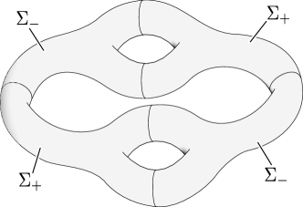
(a)

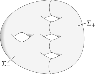
(b)

Figure 3. Surfaces $\Sigma=\Sigma_{+}\cup_{\Gamma}\Sigma_{-}$ which yield $\SS^{1}$–invariant contact manifolds $(\SS^{1}\times\Sigma,\xi_{\Gamma})$ that are weakly but not strongly fillable due to Corollary 5.

One further implication of the techniques introduced in §2 is that weak fillings can now be studied using the technology of Symplectic Field Theory. The latter is a general framework introduced by Eliashberg, Givental and Hofer [EGH00] for defining contact invariants by counting $J$–holomorphic curves in symplectizations and in noncompact symplectic cobordisms with cylindrical ends. In joint work of the second author with Janko Latschev [LW10], it is shown that SFT contains an algebraic variant of planar torsion, which gives an infinite hierarchy of obstructions to the existence of strong fillings and exact symplectic cobordisms in all dimensions. Stable Hamiltonian structures can be used to incorporate weak fillings into this picture as well: analogously to the situation in Heegaard Floer homology, the distinction between strong and weak is then seen algebraically via twisted (i.e. group ring) coefficients in SFT.

We will explain a special case of this statement in §2.5, focusing on the simplest and most widely known invariant defined within the SFT framework: contact homology. Given a contact manifold $(M,\xi)$, the contact homology ${\operatorname{HC}_{*}}\big{(}M,\xi\big{)}$ can be defined as a ${\mathbb{Z}}_{2}$–graded supercommutative algebra with unit: it is the homology of a differential graded algebra generated by Reeb orbits of a nondegenerate contact form, where the differential counts rigid $J$–holomorphic spheres with exactly one positive end and arbitrarily many negative ends. (See §2.5 for more precise definitions.) We say that the homology vanishes if it satisfies the relation ${\mathbf{1}}=0$, which implies that it contains only one element. In defining this algebra, one can make various choices of coefficients, and in particular for any linear subspace $\mathcal{R}\subset H_{2}(M;{\mathbb{R}})$, one can define contact homology as a module over the group ring

$${\mathbb{Q}}[H_{2}(M;{\mathbb{R}})/\mathcal{R}]=\left\{\sum_{i=1}^{N}c_{i}e^{A_{i}}\ \Bigm{|}\ c_{i}\in{\mathbb{Q}},\ A_{i}\in H_{2}(M;{\mathbb{R}})/\mathcal{R}\right\}\;,$$

with the differential “twisted” by inserting factors of $e^{A}$ to keep track of the homology classes of holomorphic curves. We will denote the contact homology algebra defined in this way for a given subspace $\mathcal{R}\subset H_{2}(M;{\mathbb{R}})$ by

$${\operatorname{HC}_{*}}\big{(}M,\xi;\,{\mathbb{Q}}[H_{2}(M;{\mathbb{R}})/\mathcal{R}]\big{)}\;.$$

There are two obvious special cases that must be singled out: if $\mathcal{R}=H_{2}(M;{\mathbb{R}})$, then the coefficients reduce to ${\mathbb{Q}}$, and we obtain the untwisted contact homology ${\operatorname{HC}_{*}}\big{(}M,\xi;\,{\mathbb{Q}}\big{)}$, in which the group ring does not appear. If we instead set $\mathcal{R}=\{0\}$, the result is the fully twisted contact homology ${\operatorname{HC}_{*}}\big{(}M,\xi;\,{\mathbb{Q}}[H_{2}(M;{\mathbb{R}})]\big{)}$, which is a module over ${\mathbb{Q}}[H_{2}(M;{\mathbb{R}})]$. There is also an intermediately twisted version associated to any cohomology class $\beta\in H^{2}_{\operatorname{dR}}(M)$, namely ${\operatorname{HC}_{*}}\big{(}M,\xi;\,{\mathbb{Q}}[H_{2}(M;{\mathbb{R}})/\ker\beta]\big{)}$, where we identify $\beta$ with the induced linear map $H_{2}(M;{\mathbb{R}})\to{\mathbb{R}},\,A\mapsto{\langle{\beta},{A}\rangle}$. Observe that the canonical projections ${\mathbb{Q}}[H_{2}(M;{\mathbb{R}})]\to{\mathbb{Q}}[H_{2}(M;{\mathbb{R}})/\ker\beta]\to{\mathbb{Q}}$ yield algebra homomorphisms

$${\operatorname{HC}_{*}}\big{(}M,\xi;\,{\mathbb{Q}}[H_{2}(M;{\mathbb{R}})]\big{)}\to{\operatorname{HC}_{*}}\big{(}M,\xi;\,{\mathbb{Q}}[H_{2}(M;{\mathbb{R}})/\ker\beta]\big{)}\to{\operatorname{HC}_{*}}\big{(}M,\xi;\,{\mathbb{Q}}\big{)}\;,$$

implying in particular that whenever the fully twisted version vanishes, so do all the others. The choice of twisted coefficients then has the following relevance for the question of fillability.

Theorem 6.

Suppose $(M,\xi)$ is a closed contact $3$–manifold with a cohomology class $\beta\in H^{2}_{\operatorname{dR}}(M)$ for which ${\operatorname{HC}_{*}}\big{(}M,\xi;\,{\mathbb{Q}}[H_{2}(M;{\mathbb{R}})/\ker\beta]\big{)}$ vanishes. Then $(M,\xi)$ does not admit any weak symplectic filling $(W,\omega)$ with $[{\left.{\omega}\right|_{TM}}]=\beta$.

Since weak fillings that are exact near the boundary are equivalent to strong fillings up to symplectic deformation (cf. Proposition 3.1 in [Eli91]), the special case $\beta=0$ means that the untwisted contact homology gives an obstruction to strong filling, and we similarly obtain an obstruction to weak filling from the fully twisted contact homology:

Corollary 6.

For any closed contact $3$–manifold $(M,\xi)$:

1. If ${\operatorname{HC}_{*}}\big{(}M,\xi;\,{\mathbb{Q}}\big{)}$ vanishes, then $(M,\xi)$ is not strongly fillable.

2. If ${\operatorname{HC}_{*}}\big{(}M,\xi;\,{\mathbb{Q}}[H_{2}(M;{\mathbb{R}})]\big{)}$ vanishes, then $(M,\xi)$ is not weakly fillable.

This result does not immediately yield any new knowledge about contact topology, as so far the overtwisted contact manifolds are the only examples in dimension $3$ for which any version (in particular the twisted version) of contact homology is known to vanish, cf. [Yau06] and [Wen10b]. We’ve included it here merely as a “proof of concept” for the use of SFT with twisted coefficients to study weak fillings. For the higher order algebraic filling obstructions defined in [LW10], there are indeed examples where the twisted and untwisted theories differ, corresponding to tight contact manifolds that are weakly but not strongly fillable.

We conclude this introduction with a brief discussion of open questions.

Insofar as planar torsion provides an obstruction to weak filling, it is natural to wonder how sharp the homological condition in Theorem 3 is. The most obvious test cases are the $\SS^{1}$–invariant product manifolds $(\SS^{1}\times\Sigma,\xi_{\Gamma})$, under the assumption that $\Sigma\setminus\Gamma$ contains a connected component of genus zero, as for these the question of strong fillability is completely understood by results in [Wen10b] and [Wen]. Theorems 3 and 5 give criteria when such manifolds either are or are not weakly fillable, but there is still a grey area in which neither result applies, e.g. neither is able to settle the following:

Question 1.

Suppose $\Sigma=\Sigma_{+}\cup_{\Gamma}\Sigma_{-}$, where $\Sigma\setminus\Gamma$ contains a connected component of genus zero and some connected components of $\Gamma$ separate $\Sigma$, while others do not. Is $(\SS^{1}\times\Sigma,\xi_{\Gamma})$ weakly fillable?

Another question concerns the classification of weak fillings: on rational homology spheres this reduces to a question about strong fillings, and Theorem 2 reduces it to the Stein case for all planar contact manifolds, which makes general classification results seem quite realistic. But already in the simple case of the tight $3$–tori, one can combine explicit examples such as $\Sigma\times{\mathbb{T}}^{2}$ with our splicing technique to produce a seemingly unclassifiable zoo of inequivalent weak fillings. Note that the splicing technique can be applied in general for contact manifolds that admit fillings with homologically nontrivial pre-Lagrangian tori, and these are never planar, because due to an obstruction of Etnyre [Etn04b] fillings of planar contact manifolds must have trivial $b_{2}^{0}$.

Question 2.

Other than rational homology spheres, are there any non-planar weakly fillable contact $3$–manifolds for which weak fillings can reasonably be classified?

On the algebraic side, it would be interesting to know whether Theorem 3 actually implies any contact topological results that are not known; this relates to the rather important open question of whether there exist tight contact $3$–manifolds with vanishing contact homology. In light of the role played by twisted coefficients in the distinction between strong and weak fillings, this question can be refined as follows:

Question 3.

Does there exist a tight contact $3$–manifold with vanishing (twisted or untwisted) contact homology? In particular, is there a weakly fillable contact $3$–manifold with vanishing untwisted contact homology?

The generalization of overtwistedness furnished by planar torsion gives some evidence that the answer to this last question may be no. In particular, planar torsion as defined in [Wen10b] comes with an integer-valued order $k\geq 0$, and for every $k\geq 1$, our results give examples of contact manifolds with planar $k$–torsion that are weakly but not strongly fillable. This phenomenon is also detected algebraically both by Embedded Contact Homology [Wen10b] and by Symplectic Field Theory [LW10], where in each case the untwisted version vanishes and the twisted version does not. Planar $0$–torsion, however, is fully equivalent to overtwistedness, and thus always causes the twisted theories to vanish. Thus on the $k=0$ level, there is a conspicuous lack of candidates that could answer the above question in the affirmative.

Relatedly, the distinction between twisted and untwisted contact homology makes just as much sense in higher dimensions, yet the distinction between weak and strong fillings apparently does not. The simplest possible definition of a weak filling in higher dimensions, that $\partial W=M$ with ${\left.{\omega}\right|_{\xi}}$ symplectic, is not very natural and probably cannot be used to prove anything. A better definition takes account of the fact that $\xi$ carries a natural conformal symplectic structure, and $\omega$ should be required to define the same conformal symplectic structure on $\xi$: in this case we say that $(M,\xi)$ is dominated by $(W,\omega)$. In dimension three this notion is equivalent to that of a weak filling, but surprisingly, in higher dimensions it is equivalent to strong filling, by a result of McDuff [McD91]. It is thus extremely unclear whether any sensible distinct notion of weak fillability exists in higher dimensions, except algebraically:

Question 4.

In dimensions five and higher, are there contact manifolds with vanishing untwisted but nonvanishing twisted contact homology (or similarly, algebraic torsion as in [LW10])? If so, what does this mean about their symplectic fillings?

Another natural question in higher dimensions concerns the variety of possible filling obstructions, of which very few are yet known. There are obstructions arising from the plastikstufe [Nie06], designed as a higher dimensional analog of the overtwisted disk, as well as from left handed stabilizations of open books [BvK10]. Both of these cause contact homology to vanish, and there is as yet no known example of a “higher order” filling obstruction in higher dimensions, i.e. something analogous to Giroux torsion or planar torsion, which might obstruct symplectic filling without killing contact homology. One promising avenue to explore in this area would be to produce a higher dimensional generalization of the anchored overtwisted annulus, though once an example is constructed, it may be far from trivial to show that it has nonvanishing contact homology.

Question 5.

Is there any higher dimensional analog of the anchored overtwisted annulus, and can it be used to produce examples of nonfillable contact manifolds with nonvanishing contact homology?

Acknowledgments

We are grateful to Emmanuel Giroux, Michael Hutchings and Patrick Massot for enlightening conversations.

During the initial phase of this research, K. Niederkrüger was working at the ENS de Lyon funded by the project Symplexe 06-BLAN-0030-01 of the Agence Nationale de la Recherche (ANR). Currently he is employed at the Université Paul Sabatier – Toulouse III.

C. Wendl is supported by an Alexander von Humboldt Foundation research fellowship.

1. Giroux torsion and the overtwisted annulus

In this section, which can be read independently of the remainder of the paper, we adapt the techniques used in the non-fillability proof for overtwisted manifolds due to Eliashberg and Gromov to prove Theorem 1.

We begin by briefly sketching the original proof for overtwisted contact structures. Assume $(M,\xi)$ is a closed overtwisted contact manifold with a weak symplectic filling $(W,\omega)$. The condition ${\left.{\omega}\right|_{\xi}}>0$ implies that we can choose an almost complex structure $J$ on $W$ which is tamed by $\omega$ and makes the boundary $J$–convex. The elliptic singularity in the center of the overtwisted disk ${\mathbb{D}_{\mathrm{OT}}}\subset M$ is the source of a $1$–dimensional connected moduli space ${\mathcal{M}}$ of $J$–holomorphic disks

$$u:\,\bigl{(}{\mathbb{D}},\partial{\mathbb{D}}\bigr{)}\to\bigl{(}W,{\mathbb{D}_{\mathrm{OT}}}\bigr{)}$$

that represent homotopically trivial elements in $\pi_{2}\bigl{(}W,{\mathbb{D}_{\mathrm{OT}}}\bigr{)}$, and whose boundaries encircle the singularity of ${\mathbb{D}_{\mathrm{OT}}}$ once. The space ${\mathcal{M}}$ is diffeomorphic to an open interval, and as we approach one limit of this interval the holomorphic curves collapse to the singular point in the center of the overtwisted disk ${\mathbb{D}_{\mathrm{OT}}}$.

We can add to any holomorphic disk in ${\mathcal{M}}$ a capping disk in ${\mathbb{D}_{\mathrm{OT}}}$, such that we obtain a sphere that bounds a ball, and hence the $\omega$–energy of any disk in ${\mathcal{M}}$ is equal to the symplectic area of the capping disk. This implies that the energy of any holomorphic disk in ${\mathcal{M}}$ is bounded by the integral of ${\left\lvert\omega\right\rvert}$ over ${\mathbb{D}_{\mathrm{OT}}}$, so that we can apply Gromov compactness to understand the limit at the other end of ${\mathcal{M}}$. By a careful study, bubbling and other phenomena can be excluded, and the result is a limit curve that must have a boundary point tangent to the characteristic foliation at $\partial{\mathbb{D}_{\mathrm{OT}}}$; but this implies that it touches $\partial W$ tangentially, which is impossible due to $J$–convexity.

Below we will work out an analogous proof for the situation where $(M,\xi)$ is a closed $3$–dimensional contact manifold that contains a different object, called an anchored overtwisted annulus. Assuming $(M,\xi)$ has a weak symplectic filling or is a weakly contact hypersurface in a closed symplectic $4$–manifold, we will choose an adapted almost complex structure and instead of using holomorphic disks, consider holomorphic annuli with boundaries varying along a $1$–dimensional family of surfaces. The extra degree of freedom in the boundary condition produces a moduli space of positive dimension. If $\omega$ is also exact on the region foliated by the family of boundary conditions, then we obtain an energy bound, allowing us to apply Gromov compactness and derive a contradiction.

1.1. The overtwisted annulus

We begin by introducing a geometric object that will play the role of an overtwisted disk. Recall that for any oriented surface $S\hookrightarrow M$ embedded in a contact $3$–manifold $(M,\xi)$, the intersection $TS\cap\xi$ defines an oriented singular foliation $S_{\xi}$ on $S$, called the characteristic foliation. Its leaves are oriented $1$–dimensional submanifolds, and every point where $\xi$ is tangent to $S$ yields a singularity, which can be given a sign by comparing the orientations of $\xi$ and $TS$.

Definition 1.1.

Let $(M,\xi)$ be a $3$–dimensional contact manifold. A submanifold $\mathbb{A}\cong[0,1]\times\SS^{1}\hookrightarrow M$ is called a half-twisted annulus if the characteristic foliation $\mathbb{A}_{\xi}$ has the following properties:

1. $\mathbb{A}_{\xi}$ is singular along $\{0\}\times\SS^{1}$ and regular on $(0,1]\times\SS^{1}$.

2. $\{1\}\times\SS^{1}$ is a closed leaf.

3. $(0,1)\times\SS^{1}$ is foliated by an $\SS^{1}$–invariant family of characteristic leaves that each meet $\{0\}\times\SS^{1}$ transversely and approach $\partial\mathbb{A}$ asymptotically.

We will refer to the two boundary components $\partial_{L}\mathbb{A}:=\{1\}\times\SS^{1}$ and $\partial_{S}\mathbb{A}:=\{0\}\times\SS^{1}$ as the Legendrian and singular boundaries respectively. An overtwisted annulus is then a smoothly embedded annulus $\mathbb{A}\subset M$ which is the union of two half-twisted annuli

$$\mathbb{A}=\mathbb{A}^{-}\cup\mathbb{A}^{+}$$

along their singular boundaries (see Figure 4).

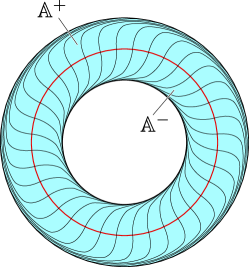
Figure 4. An overtwisted annulus $\mathbb{A}=\mathbb{A}^{-}\cup\mathbb{A}^{+}$ with its singular characteristic foliation.

Remark 1.2.

As pointed out to us by Giroux, every neighborhood of a point in a contact manifold contains an overtwisted annulus. Indeed, any knot admits a $C^{0}$–small perturbation to a Legendrian knot, which then has a neighborhood contactomorphic to the solid torus $\SS^{1}\times{\mathbb{D}}\ni(\vartheta;x,y)$ with contact structure $\ker\left(dy-x\,d\vartheta\right)$. A small torus ${\mathbb{T}}^{2}\cong\SS^{1}\times\bigl{\{}(x,y)\bigm{|}\,x^{2}+y^{2}=\varepsilon\bigr{\}}$ is composed of two annuli glued to each other along their boundaries, and the characteristic foliation on each of these is linear on the interior but singular at the boundary. By pushing one of these annuli slightly inward along one boundary component and the other slightly outward along the corresponding boundary component, we obtain an overtwisted annulus.

The above remark demonstrates that a single overtwisted annulus can never give any contact topological information. We will show however that the following much more restrictive notion carries highly nontrivial consequences.

Definition 1.3.

We will say that an overtwisted annulus $\mathbb{A}=\mathbb{A}^{-}\cup\mathbb{A}^{+}\subset(M,\xi)$ is anchored if $(M,\xi)$ contains a smooth $\SS^{1}$–parametrized family of half-twisted annuli $\bigl{\{}\mathbb{A}^{-}_{\vartheta}\bigr{\}}_{\vartheta\in\SS^{1}}$ which are disjoint from each other and from $\mathbb{A}^{+}$, such that $\mathbb{A}^{-}_{0}=\mathbb{A}^{-}$. The region foliated by $\bigl{\{}\mathbb{A}^{-}_{\vartheta}\bigr{\}}_{\vartheta\in\SS^{1}}$ is then called the anchor.

Example 1.4.

Recall that we defined a Giroux torsion domain $T_{n}$ as the thickened torus ${\mathbb{T}}^{2}\times[0,n]=\bigl{\{}(\varphi,\vartheta;z)\bigr{\}}$ with contact structure given as the kernel of

$$\sin(2\pi z)\,d\varphi+\cos(2\pi z)\,d\vartheta\;.$$

For every $\vartheta\in S^{1}$, such a torsion domain contains an overtwisted annulus $\mathbb{A}_{\vartheta}$ which we obtain by bending the image of

$$[0,1]\times\SS^{1}\hookrightarrow T_{n},\,\bigl{(}z,\varphi\bigr{)}\mapsto\bigl{(}\varphi,\vartheta;z\bigr{)}$$

slightly downward along the edges $\{0,1\}\times\SS^{1}$ so that they become regular leaves of the foliation. This can be done in such a way that ${\mathbb{T}}^{2}\times[0,1]$ is foliated by an $\SS^{1}$–family of overtwisted annuli,

$${\mathbb{T}}^{2}\times[0,1]=\bigcup_{\vartheta\in\SS^{1}}\mathbb{A}_{\vartheta}\;,$$

all of which are therefore anchored.

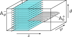
Figure 5. An anchored overtwisted annulus $\mathbb{A}=\mathbb{A}_{0}^{-}\cup\mathbb{A}_{0}^{+}$ in a Giroux torsion domain $T_{1}$.

The example shows that every contact manifold with positive Giroux torsion contains an anchored overtwisted annulus, but in fact, as John Etnyre and Patrick Massot have pointed out to us, the converse is also true: it follows from deep results concerning the classification of tight contact structures on thickened tori [Gir00] that a contact manifold must have positive Giroux torsion if it contains an anchored overtwisted annulus.

We will use an anchored overtwisted annulus as a boundary condition for holomorphic annuli. By studying the moduli space of such holomorphic curves, we find certain topological conditions that have to be satisfied by a weak symplectic filling, and which will imply Theorem 1.

1.2. The Bishop family of holomorphic annuli

In the non-fillability proof for overtwisted manifolds, the source of the Bishop family is an elliptic singularity at the center of the overtwisted disk. For an anchored overtwisted annulus, holomorphic curves will similarly emerge out of singularities of the characteristic foliation, in this case the singular boundaries of the half-twisted annuli in the anchor, which all together trace out a pre-Lagrangian torus. We shall first define a boundary value problem for pseudoholomorphic annuli with boundary in an anchored overtwisted annulus, and then choose a special almost complex structure near the singularities for which solutions to this problem can be constructed explicitly. If $\omega$ is exact on the anchor, then the resulting energy bound and compactness theorem for the moduli space will lead to a contradiction.

For the remainder of §1, suppose $(W,\omega)$ is a weak filling of $(M,\xi)$, and the latter contains an anchored overtwisted annulus $\mathbb{A}=\mathbb{A}^{-}\cup\mathbb{A}^{+}$ with anchor $\{\mathbb{A}^{-}_{\vartheta}\}_{\vartheta\in\SS^{1}}$ such that $\mathbb{A}^{-}_{0}=\mathbb{A}^{-}$. The argument will require only minor modifications for the case where $(W,\omega)$ is closed and contains $(M,\xi)$ as a weakly contact hypersurface; see Remark 1.14.

1.2.1. A boundary value problem for anchored overtwisted annuli

We will say that an almost complex structure $J$ on $W$ is adapted to the filling if it is tamed by $\omega$ and preserves $\xi$. The fact that $\xi$ is a positive contact structure implies that any $J$ adapted to the filling makes the boundary $\partial W$ pseudoconvex, with the following standard consequences:

Lemma 1.5 (cf. [Zeh03], Theorem 4.2.3).

If $J$ is adapted to the filling $(W,\omega)$ of $(M,\xi)$, then:

1. Any embedded surface $S\subset M=\partial W$ on which the characteristic foliation is regular is a totally real submanifold of $(W,J)$.

2. Any connected $J$–holomorphic curve whose interior intersects $\partial W$ must be constant.

3. If $S\subset\partial W$ is a totally real surface as described above and $u:\,\Sigma\to W$ is a $J$–holomorphic curve satisfying the boundary condition $u(\partial\Sigma)\subset S$, then $u|_{\partial\Sigma}$ is immersed and positively transverse to the characteristic foliation on $S$.

Given any adapted almost complex structure $J$ on $(W,\omega)$, the above lemma implies that the interiors $\operatorname{int}{\mathbb{A}^{+}}\subset\mathbb{A}^{+}$ and $\operatorname{int}{\mathbb{A}^{-}_{\vartheta}}\subset\mathbb{A}^{-}_{\vartheta}$ are all totally real submanifolds of $(W,J)$. We shall then consider a moduli space of $J$–holomorphic annuli defined as follows. Denote by $A_{r}$ the complex annulus

$$A_{r}=\bigl{\{}z\in{\mathbb{C}}\bigm{|}\,1\leq{\left\lvert z\right\rvert}\leq 1+r\bigr{\}}\subset{\mathbb{C}}$$

of modulus $r>0$, and write its boundary components as $\partial_{r}^{-}:=\bigl{\{}z\in{\mathbb{C}}\bigm{|}\,{\left\lvert z\right\rvert}=1\bigr{\}}$ and $\partial_{r}^{+}:=\bigl{\{}z\in{\mathbb{C}}\bigm{|}\,{\left\lvert z\right\rvert}=1+r\bigr{\}}$. We then define the space

$$\begin{split}{\mathcal{M}}(J)=\bigcup_{r>0}\bigl{\{}u:A_{r}\to W\ \bigm{|}\ &Tu\circ i=J\circ Tu,\text{ $u(\partial_{r}^{+})\subset\operatorname{int}{\mathbb{A}^{+}}$,}\\ &\text{$u(\partial_{r}^{-})\subset\operatorname{int}{\mathbb{A}^{-}_{\vartheta}}$ for any $\vartheta\in\SS^{1}$}\bigl{\}}\Big{/}\SS^{1},\end{split}$$

where $\tau\in\SS^{1}$ acts on maps $u:\,A_{r}\to W$ by $\tau\cdot u(z):=u(e^{2\pi i\tau}z)$. This space can be given a natural topology by fixing a smooth family of diffeomorphisms from a standard annulus to the domains $A_{r}$,

(1.1) $$\psi_{r}:\,[0,1]\times\SS^{1}\to A_{r}:(s,t)\mapsto e^{s\log(1+r)+2\pi it}\;,$$

and then saying that a sequence $u_{k}:A_{r_{k}}\to W$ converges to $u:\,A_{r}\to W$ in ${\mathcal{M}}(J)$ if $r_{k}\to r$ and

$$u_{k}\circ\psi_{r_{k}}(s,t+\tau_{k})\to u\circ\psi_{r}(s,t)$$

for some sequence $\tau_{k}\in\SS^{1}$, with $C^{\infty}$–convergence on $[0,1]\times\SS^{1}$.

We will show below that $J$ can be chosen to make ${\mathcal{M}}(J)$ a nonempty smooth manifold of dimension one. This explains why the “anchoring” condition is necessary: it introduces an extra degree of freedom in the boundary condition, without which the moduli space would generically be zero-dimensional and the Bishop family could never expand to reach the edge of the half-twisted annuli.

1.2.2. Special almost complex structures near the boundary

Suppose $\alpha$ is a contact form for $(M,\xi)$. The standard way to construct compatible almost complex structures on the symplectization $\bigl{(}{\mathbb{R}}\times M,d(e^{t}\alpha)\bigr{)}$ involves choosing a compatible complex structure $J_{\xi}$ on the symplectic vector bundle $\bigl{(}{\left.{\xi}\right|_{\{0\}\times M}},d\alpha\bigr{)}$, extending it to a complex structure on $\bigl{(}{\left.{T({\mathbb{R}}\times M)}\right|_{\{0\}\times M}},d(e^{t}\alpha)\bigr{)}$ such that

$$JX_{\alpha}=-\partial_{t}\text{ and }J\partial_{t}=X_{\alpha}$$

for the Reeb vector field $X_{\alpha}$ of $\alpha$, and finally defining $J$ as the unique ${\mathbb{R}}$–invariant almost complex structure on ${\mathbb{R}}\times M$ that has this form at $\{0\}\times M$. Almost complex structures of this type will be essential for the arguments of §2. For the remainder of this section, we will drop the ${\mathbb{R}}$–invariance condition but say that an almost complex structure on ${\mathbb{R}}\times M$ is compatible with $\alpha$ if it takes the above form on $\{0\}\times M$; in this case it is tamed by $d(e^{t}\alpha)$ on any sufficiently small neighborhood of $\{0\}\times M$. It is sometimes useful to know that an adapted $J$ on any weak filling can be chosen to match any given $J$ of this form near the boundary.

Proposition 1.6.

Let $(M,\xi)$ be a contact $3$–manifold with weak filling $(W,\omega)$. Choose any contact form $\alpha$ for $\xi$ and an almost complex structure $J$ on ${\mathbb{R}}\times M$ compatible with $\alpha$. Then for sufficiently small $\varepsilon>0$, the canonical identification of $\{0\}\times M$ with $\partial W$ can be extended to a diffeomorphism from $(-\varepsilon,0]\times M$ to a collar neighborhood of $\partial W$ such that the push-forward of $J$ is tamed by $\omega$.

In particular, this almost complex structure can then be extended to a global almost complex structure on $W$ that is tamed by $\omega$, and is thus adapted to the filling.

Démonstration.

Writing $J_{\xi}:={\left.{J}\right|_{\xi}}$, construct an auxiliary complex structure $J_{\mathrm{aux}}$ on ${\left.{TW}\right|_{M}}$ as the direct sum of $J_{\xi}$ on the symplectic bundle $\bigl{(}{\left.{\xi}\right|_{\{0\}\times M}},\omega\bigr{)}$ with a compatible complex structure on its $\omega$–symplectic complement $\bigl{(}{\left.{\xi^{\perp\omega}}\right|_{\{0\}\times M}},\omega\bigr{)}$. Clearly this complex structure is tamed by ${\left.{\omega}\right|_{M}}$.

Define an outward pointing vector field along the boundary by setting

$$Y=-J_{\mathrm{aux}}\cdot X_{\alpha}\;.$$

Extend $Y$ to a smooth vector field on a small neighborhood of $M$ in $W$, and use its flow to define an embedding of a subset of the symplectization

$$\Psi:\,(-\varepsilon,0]\times M\to W,\,\bigl{(}t,p\bigr{)}\mapsto\Phi_{Y}^{t}(p)$$

for sufficiently small $\varepsilon>0$. The restriction of $\Psi$ to $\{0\}\times M$ is the identity on $M$, and the push-forward of $J$ under this map coincides with $J_{\mathrm{aux}}$ along $M$, because $\Psi_{*}\partial_{t}=Y$. It follows that the push-forward of $J$ is tamed by $\omega$ on a sufficiently small neighborhood of $M=\partial W$, and we can then extend it to $W$ as an almost complex structure tamed by $\omega$. ∎

1.2.3. Generation of the Bishop family

We shall now choose an almost complex structure $J_{0}$ on the symplectization of $M$ that allows us to write down the germ of a Bishop family in ${\mathbb{R}}\times M$ which generates a component of ${\mathcal{M}}(J_{0})$. At the same time, $J_{0}$ will prevent other holomorphic curves in the same component of ${\mathcal{M}}(J_{0})$ from approaching the singular boundaries of the half-twisted annuli $\mathbb{A}^{-}_{\vartheta}$. We can then apply Proposition 1.6 to identify a neighborhood of $\{0\}\times M$ in the symplectization with a boundary collar of $W$, so that $W$ contains the Bishop family.

The singular boundaries of $\mathbb{A}^{-}_{\vartheta}$ define closed leaves of the characteristic foliation on a torus

$$T:=\bigcup_{\vartheta\in\SS^{1}}\partial_{S}\mathbb{A}^{-}_{\vartheta}\subset M\;,$$

which is therefore a pre-Lagrangian torus. We then obtain the following by a standard Moser-type argument.

Lemma 1.7.

For sufficiently small $\varepsilon>0$, a tubular neighborhood $\mathcal{N}(T)\subset M$ of $T$ can be identified with ${\mathbb{T}}^{2}\times(-\varepsilon,\varepsilon)$ with coordinates $(\varphi,\vartheta;r)$ such that:

• $T={\mathbb{T}}^{2}\times\{0\}$,

• $\xi=\ker\left[\cos(2\pi r)\,d\vartheta+\sin(2\pi r)\,d\varphi\right]$,

• $\mathbb{A}\cap\mathcal{N}(T)=\{\vartheta=0\}$, and $\mathbb{A}^{-}_{\vartheta_{0}}\cap\mathcal{N}(T)=\{\vartheta=\vartheta_{0},\ r\in(-\varepsilon,0]\}$ for all $\vartheta_{0}\in\SS^{1}$.

Using the coordinates given by the lemma, we can reflect the half-twisted annuli $\mathbb{A}^{-}_{\vartheta_{0}}$ across $T$ within this neighborhood to define the surfaces

$$\mathbb{A}^{+}_{\vartheta_{0}}:=\bigl{\{}\vartheta=\vartheta_{0},\ r\in[0,\varepsilon)\bigr{\}}\subset M\;.$$

Each of these surfaces looks like a collar neighborhood of the singular boundary in a half-twisted annulus. Now choose for $\xi$ a contact form $\alpha$ on $M$ that restricts on $\mathcal{N}(T)$ to

(1.2) $${\left.{\alpha}\right|_{\mathcal{N}(T)}}=\cos(2\pi r)\,d\vartheta+\sin(2\pi r)\,d\varphi\;.$$

The main idea of the construction is to identify the set $\mathcal{N}(T)$ with an open subset of the unit cotangent bundle ${\mathbb{T}}^{3}=\SS\bigl{(}T^{*}{\mathbb{T}}^{2}\bigr{)}$ of ${\mathbb{T}}^{2}$, with its canonical contact form ${\alpha_{\mathrm{can}}}$. We will then use an integrable complex structure on $T^{*}{\mathbb{T}}^{2}$ to find explicit families of holomorphic curves that give rise to holomorphic annuli in ${\mathbb{R}}\times M$.

The cotangent bundle of ${\mathbb{T}}^{2}={\mathbb{R}}^{2}/{\mathbb{Z}}^{2}$ can be identified naturally with

$${\mathbb{C}}^{2}/i{\mathbb{Z}}^{2}={\mathbb{R}}^{2}\oplus i({\mathbb{R}}^{2}/{\mathbb{Z}}^{2})$$

such that the canonical $1$–form takes the form ${\lambda_{\mathrm{can}}}=p_{1}\,dq_{1}+p_{2}\,dq_{2}$ in coordinates $[z_{1},z_{2}]=\bigl{[}p_{1}+iq_{1},p_{2}+iq_{2}\bigr{]}$. The unit cotangent bundle $\SS\bigl{(}T^{*}{\mathbb{T}}^{2}\bigr{)}=\bigl{\{}[p_{1}+iq_{1},p_{2}+iq_{2}]\in T^{*}{\mathbb{T}}^{2}\bigm{|}\,{\left\lvert p_{1}\right\rvert}^{2}+{\left\lvert p_{2}\right\rvert}^{2}=1\bigr{\}}$ can then be parametrized by the map

$${\mathbb{T}}^{3}={\mathbb{T}}^{2}\times\SS^{1}\ni(\varphi,\vartheta;r)\mapsto\bigl{[}\sin 2\pi r+i\varphi,\cos 2\pi r+i\vartheta\bigr{]}\in T^{*}{\mathbb{T}}^{2}\;,$$

and the pull-back of ${\lambda_{\mathrm{can}}}$ to ${\mathbb{T}}^{3}$ gives

$${\alpha_{\mathrm{can}}}:={\left.{{\lambda_{\mathrm{can}}}}\right|_{T\SS(T^{*}{\mathbb{T}}^{2})}}=\cos(2\pi r)\,d\vartheta+\sin(2\pi r)\,d\varphi\;.$$

The Liouville vector field dual to ${\lambda_{\mathrm{can}}}$ is $p_{1}\,\partial_{p_{1}}+p_{2}\,\partial_{p_{2}}$, and we can use its flow to identify $T^{*}{\mathbb{T}}^{2}\setminus{\mathbb{T}}^{2}$ with the symplectization of $\SS\bigl{(}T^{*}{\mathbb{T}}^{2}\bigr{)}$:

$$\Phi:\,({\mathbb{R}}\times\SS\bigl{(}T^{*}{\mathbb{T}}^{2}\bigr{)},d(e^{t}{\alpha_{\mathrm{can}}}))\to(T^{*}{\mathbb{T}}^{2}\setminus{\mathbb{T}}^{2},d{\lambda_{\mathrm{can}}}),\,(t;p+iq)\mapsto e^{t}p+iq\;.$$

Then it is easy to check that the restriction of the complex structure $\Phi^{*}i$ to $\{0\}\times{\mathbb{T}}^{3}$ preserves $\ker{\alpha_{\mathrm{can}}}$ and maps $\partial_{t}$ to the Reeb vector field of ${\alpha_{\mathrm{can}}}$, hence $\Phi^{*}i$ is compatible with ${\alpha_{\mathrm{can}}}$. Now for the neighborhood $\mathcal{N}(T)\cong{\mathbb{T}}^{2}\times(-\varepsilon,\varepsilon)$, denote by

$$\Psi:\,(-\varepsilon,0]\times\mathcal{N}(T)\hookrightarrow{\mathbb{R}}\times{\mathbb{T}}^{3}$$

the natural embedding determined by the coordinates $(\varphi,\vartheta;r)$. Proposition 1.6 then implies:

Lemma 1.8.

There exists an almost complex structure $J_{0}$ adapted to the filling $(W,\omega)$ of $(M,\xi)$, and a collar neighborhood $\mathcal{N}(\partial W)\cong(-\varepsilon,0]\times M$ of $\partial W$ such that on $(-\varepsilon,0]\times\mathcal{N}(T)\subset W$, $J_{0}=\Psi^{*}\Phi^{*}i$.

Consider the family of complex lines $L_{\zeta}:=\bigl{\{}(z_{1},z_{2})\bigm{|}\,z_{2}=\zeta\bigr{\}}$ in ${\mathbb{C}}^{2}$. The projection of these curves into $T^{*}{\mathbb{T}}^{2}\cong{\mathbb{C}}^{2}/i{\mathbb{Z}}^{2}$ are holomorphic cylinders, whose intersections with the unit disk bundle ${\mathbb{D}}(T^{*}{\mathbb{T}}^{2})=\bigl{\{}p+iq\in{\mathbb{C}}^{2}/i{\mathbb{Z}}^{2}\ \bigm{|}\ {\left\lvert p\right\rvert}^{2}\leq 1\bigr{\}}$ define holomorphic annuli. In particular, for sufficiently small $\delta>0$ and any

$$(c,\tau)\in(0,\delta]\times\SS^{1}\;,$$

the intersection $L_{(1-c)+i\tau}\cap{\mathbb{D}}(T^{*}{\mathbb{T}}^{2})$ is a holomorphic annulus in $\Phi\circ\Psi\bigl{(}(-\varepsilon,0]\times\mathcal{N}(T)\bigr{)}$, which therefore can be identified with a $J_{0}$–holomorphic annulus

$$u_{(c,\tau)}:\,A_{r_{c}}\to W$$

with image in the neighborhood $(-\varepsilon,0]\times\mathcal{N}(T)$, where the modulus $r_{c}>0$ depends on $c$ and approaches zero as $c\to 0$. It is easy to check that the two boundary components of $u_{(c,\tau)}$ map into the interiors of the surfaces $\mathbb{A}^{+}_{\tau}$ and $\mathbb{A}^{-}_{\tau}$ respectively in $\partial W$. Observe that all of these annuli are obviously embedded, and they foliate a neighborhood of $T$ in $W$. We summarize the construction as follows.

Proposition 1.9.

For the almost complex structure $J_{0}$ given by Lemma 1.8, there exists a smooth family of properly embedded $J_{0}$–holomorphic annuli

$$\bigl{\{}u_{(c,\tau)}:\,A_{r_{c}}\to W\bigr{\}}_{(c,\tau)\in(0,\delta]\times\SS^{1}}$$

which foliate a neighborhood of $T$ in $W\setminus T$ and satisfy the boundary conditions

$$u_{(c,\tau)}\left(\partial_{r_{c}}^{+}\right)\subset\operatorname{int}{\mathbb{A}^{+}_{\tau}},\qquad u_{(c,\tau)}\left(\partial_{r_{c}}^{-}\right)\subset\operatorname{int}{\mathbb{A}^{-}_{\tau}}.$$

In particular the curves $u_{(c,0)}$ for $c\in(0,\delta]$ all belong to the moduli space ${\mathcal{M}}(J_{0})$.

Figure 6. The unit disk bundle in $T^{*}{\mathbb{T}}^{2}$ is foliated by a family of holomorphic annuli obtained from the complex planes $L_{\zeta}$. The neighborhood $\mathcal{N}(T)$ can be identified with a subset of the unit disk bundle $\SS\bigl{(}T^{*}{\mathbb{T}}^{2}\bigr{)}$.

Denote the neighborhood foliated by the curves $u_{(c,\tau)}$ by

$${\mathcal{U}}=\bigcup_{(c,\tau)\in(0,\delta]\times\SS^{1}}u_{(c,\tau)}(A_{r_{c}})\;,$$

and define the following special class of almost complex structures,

$${\mathcal{J}}_{\mathcal{U}}(\omega,\xi)=\bigl{\{}\text{almost complex structures\leavevmode\nobreak\ $J$ adapted to the filling $(W,\omega)$ such that $J\equiv J_{0}$ on\leavevmode\nobreak\ $\overline{{\mathcal{U}}}$}\bigr{\}}\;.$$

The annuli $u_{(c,\tau)}$ are thus $J$–holomorphic for any $J\in{\mathcal{J}}_{\mathcal{U}}(\omega,\xi)$, and the space ${\mathcal{M}}(J)$ is therefore nonempty. In this case, denote by

$${\mathcal{M}}_{0}(J)\subset{\mathcal{M}}(J)$$

the connected component of ${\mathcal{M}}(J)$ that contains the curves $u_{(c,0)}$.

Lemma 1.10.

Every curve $u:A_{r}\to W$ in ${\mathcal{M}}_{0}(J)$ is proper, and its restriction to $\partial A_{r}$ is embedded.

Démonstration.

Properness follows immediately from Lemma 1.5, and due to our assumptions on the characteristic foliation of a half-twisted annulus, embeddedness at the boundary also follows from the lemma after observing that the homotopy class of $u|_{\partial_{r}^{\pm}}$ is the same as for the curves $u_{(c,0)}$, whose boundaries intersect every characteristic leaf once. ∎

Proposition 1.11.

For $J\in{\mathcal{J}}_{\mathcal{U}}(\omega,\xi)$, suppose $u\in{\mathcal{M}}_{0}(J)$ is not one of the curves $u_{(c,0)}$. Then $u$ does not intersect the interior of ${\mathcal{U}}$.

Démonstration.

The proof is based on an intersection argument. Each of the curves $u_{(c,\tau)}$ foliating ${\mathcal{U}}$ can be capped off to a cycle $\widehat{u}_{(c,\tau)}$ that represents the trivial homology class in $H_{2}(W)$. We shall proceed in a similar way to obtain a cycle $\widehat{u}$ for $u$, arranged such that intersections between the cycles $\widehat{u}$ and $\widehat{u}_{(c,\tau)}$ can only occur when the actual holomorphic curves $u$ and $u_{(c,\tau)}$ intersect. Then if $u$ is not any of the curves $u_{(c,0)}$ but intersects the interior of ${\mathcal{U}}$, it also is not a multiple cover of any $u_{(c,0)}$ due to Lemma 1.10, and therefore must have an isolated positive intersection with some curve $u_{(c,\tau)}$. It follows that $[\widehat{u}_{c_{0}}]\bullet[\widehat{u}]>0$, but since $[\widehat{u}_{c_{0}}]=0\in H_{2}(W)$, this is a contradiction.

We construct the desired caps as follows. Suppose $u(\partial^{-}_{r})\subset\mathbb{A}^{-}_{\vartheta_{0}}$. We may assume without loss of generality that $u$ and $u_{(c,\tau)}$ intersect each other in the interior, and since this intersection will not disappear under small perturbations, we can adjust $\tau$ so that it equals neither $0$ nor $\vartheta_{0}$. A cap for $u_{(c,\tau)}$ can then be constructed by filling in the space in $\mathbb{A}^{-}_{\tau}\cup\mathbb{A}^{+}_{\tau}$ between the two boundary components of $u_{(c,\tau)}$; clearly the resulting homology class $[\widehat{u}_{(c,\tau)}$] is trivial.

The cap for $u$ will be a piecewise smooth surface in $\partial W$ constructed out of three smooth pieces:

• A subset of $\mathbb{A}^{+}$ filling the space between the singular boundary $\partial_{S}\mathbb{A}^{+}$ and $u(\partial^{+}_{r})$,

• A subset of $\mathbb{A}^{-}_{\vartheta_{0}}$ filling the space between the singular boundary $\partial_{S}\mathbb{A}^{-}_{\vartheta_{0}}$ and $u(\partial^{-}_{r})$,

• An annulus in $T=\{r=0\}$ defined by letting $\vartheta$ vary over a path in $\SS^{1}$ that connects $0$ to $\vartheta_{0}$ by moving in a direction such that it does not hit $\tau$.

By construction, the two caps are disjoint, and since both are contained in $\partial W$, neither intersects the interior of either curve. ∎

1.2.4. Local structure of the moduli space

We now show that ${\mathcal{M}}_{0}(J)$ can be given a nice local structure for generic data.

Proposition 1.12.

For generic $J\in{\mathcal{J}}_{\mathcal{U}}(\omega,\xi)$, the moduli space ${\mathcal{M}}_{0}(J)$ is a smooth $1$–dimensional manifold.

Démonstration.

Since ${\mathcal{M}}_{0}(J)$ is connected by assumption, the dimension can be derived by computing the Fredholm index of the associated linearized Cauchy-Riemann operator for any of the curves $u_{(c,0)}\in{\mathcal{M}}_{0}(J)$. By Lemma 1.10, every curve $u\in{\mathcal{M}}_{0}(J)$ is somewhere injective, thus standard arguments as in [MS04] imply that for generic $J\in{\mathcal{J}}_{\mathcal{U}}(\omega,\xi)$, the subset of curves in ${\mathcal{M}}_{0}(J)$ that are not completely contained in $\overline{{\mathcal{U}}}$ is a smooth manifold of the correct dimension. Proposition 1.11 implies that the remaining curves all belong to the family $u_{(c,0)}$, and for these we will have to examine the Cauchy-Riemann operator more closely since $J$ cannot be assumed to be generic in $\overline{{\mathcal{U}}}$.

Abbreviate $u=u_{(c,0)}:\,A_{r}\to W$ for any $c\in(0,\delta]$. Since $u$ is embedded, a neighborhood of $u$ in ${\mathcal{M}}_{0}(J)$ can be described via the normal Cauchy-Riemann operator (cf. [Wen10a]),

(1.3) $$\mathbf{D}_{u}^{N}:\,W^{1,p}_{\ell,\zeta}(N_{u})\to L^{p}\bigl{(}\overline{\operatorname{Hom}}_{\mathbb{C}}(TA_{r},N_{u})\bigr{)}\;,$$

where $p>2$, $N_{u}\to A_{r}$ is the complex normal bundle of $u$, $\mathbf{D}_{u}^{N}$ is the normal part of the restriction of the usual linearized Cauchy-Riemann operator $D\bar{\partial}_{J}(u)$ (which acts on sections of $u^{*}TW$) to sections of $N_{u}$, and the subscripts $\ell$ and $\zeta$ represent a boundary condition to be described below. We must define the normal bundle $N_{u}$ so that at the boundary its intersection with $T\mathbb{A}$ has real dimension one, thus defining a totally real subbundle

$$\ell=N_{u}|_{\partial A_{r}}\cap(u|_{\partial A_{r}})^{*}T\mathbb{A}\subset N_{u}|_{\partial A_{r}}\;.$$

To be concrete, note that in the coordinates $(\varphi,\vartheta;r)$ on $\mathcal{N}(T)$, the image of $u$ can be parametrized by a map of the form

$$v:\,[-r_{0},r_{0}]\times\SS^{1}\to(-\varepsilon,0]\times\mathcal{N}(T),\,(\sigma,\tau)\mapsto(a(\sigma);\tau,0;\sigma)$$

for some $r_{0}>0$, where $a(\sigma)$ is a smooth, convex and even function. Choose a vector field along $v$ of the form

$$\nu(\sigma,\tau)=\nu_{1}(\sigma)\,\partial_{r}+\nu_{2}(\sigma)\,\partial_{t}$$

which is everywhere transverse to the path $\sigma\mapsto(a(\sigma),\sigma)$ in the $tr$–plane, and require

$$\nu(\pm r_{0},\tau)=\mp\partial_{r}\;.$$

Then the vector fields $\nu$ and $i\nu$ along $v$ span a complex line bundle that is everywhere transverse to $v$, and its intersection with $T\mathbb{A}$ at the boundary is spanned by $\partial_{r}$. We define this line bundle to be the normal bundle $N_{u}$ along $u$, which comes with a global trivialization defined by the vector field $\nu$, for which we see immediately that both components of the real subbundle $\ell$ along $\partial A_{r}$ have vanishing Maslov index. To define the proper linearized boundary condition, we still must take account of the fact that the image of $\partial^{-}_{r}$ for nearby curves in the moduli space may lie in different half-annuli $\mathbb{A}^{-}_{\vartheta}$: this means there is a smooth section $\zeta\in\Gamma(N_{u}|_{\partial^{-}_{r}})$ which is everywhere transverse to $\ell$, such that the domain for $\mathbf{D}_{u}^{N}$ takes the form

$$\begin{split}W^{1,p}_{\ell,\zeta}(N_{u}):=\bigl{\{}\eta\in W^{1,p}(N_{u})\ \bigm{|}\ &\text{$\eta(z)\in\ell_{z}$ for all $z\in\partial^{+}_{r}$},\\ &\text{$\eta(z)+c\,\zeta(z)\in\ell_{z}$ for all $z\in\partial^{-}_{r}$ and any constant $c\in{\mathbb{R}}$}\bigr{\}}\;.\end{split}$$

Leaving out the section $\zeta$, we obtain the standard totally real boundary condition

$$W^{1,p}_{\ell}(N_{u}):=\{\eta\in W^{1,p}(N_{u})\ |\ \text{$\eta(z)\in\ell_{z}$ for all $z\in\partial A_{r}$}\}\;,$$

and the Riemann-Roch formula implies that the restriction of $\mathbf{D}^{N}_{u}$ to this smaller space has Fredholm index $0$. Since the smaller space has codimension one in $W^{1,p}_{\ell,\zeta}(N_{u})$, the index of $\mathbf{D}^{N}_{u}$ on the latter is $1$, which proves the dimension formula for ${\mathcal{M}}_{0}(J)$. Moreover, since $N_{u}$ has complex rank one, there are certain automatic transversality theorems that apply: in particular, Theorem 4.5.36 in [Wen05] implies that (1.3) is always surjective, and ${\mathcal{M}}_{0}(J)$ is therefore a smooth manifold of the correct dimension, even in the region where $J$ is not generic. ∎

1.2.5. Energy bounds

Assume now that $\omega$ is exact on the anchor, i.e. there exists a $1$–form $\beta$ on the region $\bigcup_{\vartheta\in\SS^{1}}\mathbb{A}^{-}_{\vartheta}$ with $d\beta=\omega$. The aim of this section is to find a uniform bound on the $\omega$–energy

$$E_{\omega}(u)=\int_{A_{r}}u^{*}\omega$$

for all curves

$$u:\,\bigl{(}A_{r},\partial_{r}^{-}\cup\partial_{r}^{+}\bigr{)}\to(W,\mathbb{A}^{-}_{\vartheta}\cup\mathbb{A}^{+})$$

in the connected moduli space ${\mathcal{M}}_{0}(J)$ generated by the Bishop family.

Given such a curve $u\in{\mathcal{M}}_{0}(J)$, there exists a smooth $1$–parameter family of maps

$$\{u_{t}:\,A_{r}\to W\}_{t\in[\varepsilon,1]}\;,$$

such that $u_{\varepsilon}$ is a reparametrization one of the explicitly constructed curves $u_{(c,0)}$ that foliate ${\mathcal{U}}$, and $u_{1}=u$. The map $\bar{u}:[\varepsilon,1]\times A_{r}\to W:(t,z)\mapsto u_{t}(z)$ then represents a $3$–chain, and applying Stokes’ theorem to the integral of $d(\bar{u}^{*}\omega)=0$ over $[\varepsilon,1]\times A_{r}$ gives

$$E_{\omega}(u)=E_{\omega}(u_{\varepsilon})-\int_{[\varepsilon,1]\times\partial A_{r}}\bar{u}^{*}\omega\;.$$

The image $\bar{u}\bigl{(}[\varepsilon,1]\times\partial A_{r}\bigr{)}$ has two components $\bar{u}\bigl{(}[\varepsilon,1]\times\partial_{r}^{+}\bigr{)}$ and $\bar{u}\bigl{(}[\varepsilon,1]\times\partial_{r}^{-}\bigr{)}$. The first lies in a single half-twisted annulus $\mathbb{A}^{+}$, and thus the absolute value of $\int_{[\varepsilon,1]\times\partial_{r}^{+}}\bar{u}^{*}\omega$ can be bounded by $\int_{\mathbb{A}^{+}}{\left\lvert\omega\right\rvert}$. For the second component, the image $\bar{u}\bigl{(}[\varepsilon,1]\times\partial_{r}^{-}\bigr{)}$ lies in the anchor $\bigcup_{\vartheta\in\SS^{1}}\mathbb{A}^{-}_{\vartheta}$, so we can write

$$E_{\omega}(u)\leq E_{\omega}(u_{\varepsilon})+\int_{\mathbb{A}^{+}}{\left\lvert\omega\right\rvert}+\int_{\partial_{\varepsilon}^{-}}u_{\varepsilon}^{*}\beta-\int_{\partial_{r}^{-}}u^{*}\beta\;.$$

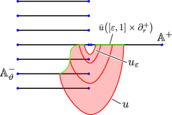
Figure 7. The holomorphic annulus $u:\,\bigl{(}A_{r},\partial_{r}^{-}\cup\partial_{r}^{+}\bigr{)}\to(W,\mathbb{A}_{\vartheta}^{-}\cup\mathbb{A}^{+})$ is part of a $1$–parameter family $u_{t}$ of curves that start at an annulus $u_{\varepsilon}$ that lies in the Bishop family.

It remains only to find a uniform bound on the last term in this sum, $\int_{\partial_{r}^{-}}u^{*}\beta$. Observe that $u(\partial_{r}^{-})$ and the singular boundary $\partial_{S}\mathbb{A}^{-}_{\vartheta}$ enclose an annulus within $\mathbb{A}^{-}_{\vartheta}$, thus

$${\left\lvert\int_{\partial_{r}^{+}}u^{*}\beta\right\rvert}\leq\int_{\partial_{S}\mathbb{A}^{-}_{\vartheta}}{\left\lvert\beta\right\rvert}+\int_{\mathbb{A}^{-}_{\vartheta}}{\left\lvert\omega\right\rvert}\;.$$

This last sum is uniformly bounded since the surfaces $\mathbb{A}^{-}_{\vartheta}$ for $\vartheta\in\SS^{1}$ form a compact family.

1.2.6. Gromov compactness for the holomorphic annuli

The main technical ingredient still needed for the proof of Theorem 1 is the following application of Gromov compactness.

Proposition 1.13.

Suppose $J$ is generic in ${\mathcal{J}}_{\mathcal{U}}(\omega,\xi)$, $\omega$ is exact on the anchor, and

$$u_{k}:\,\bigl{(}A_{r_{k}},\partial_{r_{k}}^{-}\cup\partial_{r_{k}}^{+}\bigr{)}\to(W,\mathbb{A}^{-}_{\vartheta_{k}}\cup\mathbb{A}^{+})$$

is a sequence of curves in ${\mathcal{M}}_{0}(J)$ with images not contained in ${\mathcal{U}}$. Then there exist $r>0$, $\vartheta\in\SS^{1}$ and a sequence $\tau_{k}\in\SS^{1}$ such that after passing to a subsequence, $r_{k}\to r$, $\vartheta_{k}\to\vartheta$ and the maps

$$z\mapsto u_{k}(e^{2\pi i\tau_{k}}z)$$

are $C^{\infty}$–convergent to a $J$–holomorphic annulus $u:\,A_{r}\to W$ satisfying $u(\partial^{-}_{r})\subset\mathbb{A}^{-}_{\vartheta}$ and $u(\partial^{+}_{r})\subset\mathbb{A}^{+}$.

The energies $\int_{A_{r_{k}}}u_{k}^{*}\omega$ are uniformly bounded due to the exactness assumption, and the proof is then essentially the same as in the disk case, cf. [Eli90a] or [Zeh03]. A priori, $u_{k}$ could converge to a nodal holomorphic annulus, with nodes on both the boundary and the interior. Boundary nodes are impossible however for topological reasons, as each boundary component of $u_{k}$ must pass exactly once through each leaf in an $\SS^{1}$–family of characteristic leaves, and any boundary component in a nodal annulus will also pass at least once through each of these leaves. Having excluded boundary nodes, $u_{k}$ could converge to a bubble tree consisting of holomorphic spheres and either an annulus or a pair of disks, all connected to each other by interior nodes. This however is a codimension $2$ phenomenon, and thus cannot happen for generic $J$ since ${\mathcal{M}}_{0}(J)$ is $1$–dimensional. Here we make use of two important facts:

1. Any component of the limit that has nonempty boundary must be somewhere injective, as it will be embedded at the boundary by the same argument as in Lemma 1.10. Such components therefore have nonnegative index.

2. $(W,\omega)$ is semipositive (as is always the case in dimension $4$), hence holomorphic spheres of negative index cannot bubble off.

With this, the proof of Proposition 1.13 is complete.

1.2.7. Proof of Theorem 1

Assume $(W,\omega)$ is a weak filling of $(M,\xi)$ and the latter has positive Giroux torsion. As shown in Example 1.4, $(M,\xi)$ contains an anchored overtwisted annulus. For this setting, we defined in §1.2.1 a moduli space of $J$–holomorphic annuli ${\mathcal{M}}(J)$ with a $1$–parameter family of totally real boundary conditions. In §1.2.3, we found a special almost complex structure $J_{0}$ which admits a Bishop family of holomorphic annuli, and thus generates a nonempty connected component ${\mathcal{M}}_{0}(J_{0})\subset{\mathcal{M}}(J_{0})$. This space remains nonempty after perturbing $J_{0}$ generically outside the region foliated by the Bishop family, thus producing a new almost complex structure $J$ and nonempty moduli space ${\mathcal{M}}_{0}(J)$. We then showed in §1.2.4 that ${\mathcal{M}}_{0}(J)$ is a smooth $1$–dimensional manifold, which is therefore diffeomorphic to an open interval, one end of which corresponds to the collapse of the Bishop annuli into the singular circle at the center of the overtwisted annulus. In particular, this implies that ${\mathcal{M}}_{0}(J)$ is not compact, and the key is then to understand its behavior at the other end. The assumption that $\omega$ is exact on the anchor provides a uniform energy bound, with the consequence that if all curves in $u$ remain a uniform positive distance away from the Legendrian boundaries of $\mathbb{A}^{+}$ and $\mathbb{A}^{-}_{\vartheta}$, Proposition 1.13 implies ${\mathcal{M}}_{0}(J)$ is compact. But since the latter is already known to be false, this implies that ${\mathcal{M}}_{0}(J)$ contains a sequence of curves drawing closer to the Legendrian boundary, and applying Proposition 1.13 again, a subsequence converges to a $J$–holomorphic annulus that touches the Legendrian boundary of $\mathbb{A}^{+}$ or $\mathbb{A}^{-}_{\vartheta}$ tangentially. That is impossible by Lemma 1.5, and we have a contradiction. Together with the following remark, this completes the proof of Theorem 1.

Remark 1.14.

If $(M,\xi)\subset(W,\omega)$ is a separating hypersurface of weak contact type, then half of $(W,\omega)$ is a weak filling of $(M,\xi)$ and the above argument provides a contradiction. To finish the proof of the theorem, it thus remains to show that $(M,\xi)$ under the given assumptions can never occur as a nonseparating hypersurface of weak contact type in any closed symplectic $4$–manifold $(W,\omega)$. This follows from almost the same argument, due to the following trick introduced in [ABW10]. If $M$ does not separate $W$, then we can cut $W$ open along $M$ to produce a connected symplectic cobordism $(W_{0},\omega_{0})$ between $(M,\xi)$ and itself, and then attach an infinite chain of copies of this cobordism to obtain a noncompact symplectic manifold $(W_{\infty},\omega_{\infty})$ with weakly contact boundary $(M,\xi)$. Though noncompact, $(W_{\infty},\omega_{\infty})$ is geometrically bounded in a certain sense, and an argument in [ABW10] uses the monotonicity lemma to show that for a natural class of adapted almost complex structures on $W_{\infty}$, any connected moduli space of $J$–holomorphic curves with boundary on $\partial W_{\infty}$ and uniformly bounded energy also satisfies a uniform $C^{0}$–bound. In light of this, the above argument for the compact filling also works in the “noncompact filling” furnished by $(W_{\infty},\omega_{\infty})$, thus proving that $(M,\xi)$ cannot occur as a nonseparating weakly contact hypersurface.

We will use this same trick again in the proof of Theorem 3. In relation to Theorem 2, it also implies that in any closed symplectic $4$–manifold, a weakly contact hypersurface that is planar must always be separating. This is closely related to Etnyre’s theorem [Etn04b] that planar contact manifolds never admit weak semifillings with disconnected boundary, which also can be shown using holomorphic curves, by a minor variation on the proof of Theorem 2.

Remark 1.15.

It should be possible to generalize the Bishop family idea still further by considering “overtwisted planar surfaces” with arbitrarily many boundary components (Figure 8). The disk or annulus would then be replaced by a $k$–holed sphere $\Sigma$ for some integer $k\geq 1$, with Legendrian boundary, of which $k-1$ of the boundary components are “anchored” by $\SS^{1}$–families of half-twisted annuli. The characteristic foliation on $\Sigma$ must in general have $k-2$ hyperbolic singular points. One would then find Bishop families of annuli near the anchored boundary components, which eventually must collide with each other and could be glued at the hyperbolic singularities to produce more complicated $1$–dimensional families of rational holomorphic curves with multiple boundary components, leading in the end to a more general filling obstruction.

One situation where such an object definitely exists is in the presence of planar torsion (see §2.3), though we will not pursue this approach here, as that setting lends itself especially well to the punctured holomorphic curve techniques explained in the next section.

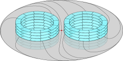
Figure 8. An overtwisted planar surface anchored at two boundary components.

2. Punctured pseudoholomorphic curves and weak fillings

We begin this section by showing that up to symplectic deformation, every weak filling can be enlarged by symplectically attaching a cylindrical end in which the theory of finite energy punctured $J$–holomorphic curves is well behaved. This fact is standard in the case where the symplectic form is exact near the boundary: indeed, Eliashberg [Eli91] observed that if $(W,\omega)$ is a weak filling of $(M,\xi)$ and $H^{2}_{\operatorname{dR}}(M)=0$, then one can always deform $\omega$ in a collar neighborhood of $\partial W$ to produce a strong filling of $(M,\xi)$, which can then be attached smoothly to a half-symplectization of the form $\bigl{(}[0,\infty)\times M,d(e^{t}\alpha)\bigr{)}$. For obvious cohomological reasons, this is not possible whenever $[{\left.{\omega}\right|_{M}}]\neq 0\in H^{2}_{\operatorname{dR}}(M)$. The solution is to work in the more general context of stable Hamiltonian structures, in which $M$ carries a closed maximal rank $2$–form that is not required to be exact. We will recall in §2.1 the important properties of stable hypersurfaces and stable Hamiltonian structures, proving in particular (Proposition 2.6) that there exist stable Hamiltonian structures representing every de Rham cohomology class. We will then use this in §2.2 to prove Theorem 2.9, that weak boundaries can always be deformed to stable hypersurfaces. A quick review of the definition and essential facts about planar torsion will then be given in §2.3, leading in §2.4 to the proofs of Theorems 2 and 3.

2.1. Stable hypersurfaces and stable Hamiltonian structures

Let us recall some important definitions. The first originates in [HZ94].

Definition 2.1.

Given a symplectic manifold $(W,\omega)$, a hypersurface $M$ is called stable if it is transverse to a vector field $Y$ defined near $M$ whose flow $\Phi^{t}_{Y}$ for small ${\left\lvert t\right\rvert}$ preserves characteristic line fields, i.e. if $M_{t}:=\Phi^{t}_{Y}(M)$ and $\ell_{t}\subset TM_{t}$ is the kernel of ${\left.{\omega}\right|_{TM_{t}}}$, then $(\Phi^{t}_{Y})_{*}\ell_{0}=\ell_{t}$.

As an important special case, if $(W,\omega)$ is a strong filling of $(M,\xi)$, then $\partial W$ is stable, as it is transverse to an outward pointing Liouville vector field which dilates $\omega$ and therefore preserves characteristic line fields. In this case we say the boundary of $W$ is convex; if $\partial W$ is instead transverse to an inward pointing Liouville vector field, we say it is concave.

Stable hypersurfaces were initially introduced in order to study dynamical questions, but it was later recognized that they also yield suitable settings for the theory of punctured $J$–holomorphic curves. In this context, the following more intrinsic notion was introduced in [BEH⁺03].

Definition 2.2.

A stable Hamiltonian structure on an oriented $3$–manifold $M$ is a pair

$$\mathcal{H}=(\lambda,\Omega)$$

consisting of a $1$–form $\lambda$ and $2$–form $\Omega$ such that

1. $d\Omega=0$,

2. $\lambda\wedge\Omega>0$,

3. $\ker\Omega\subset\ker(d\lambda)$.

The second condition implies that $\Omega$ has maximal rank and is nondegenerate on the distribution

$$\xi:=\ker\lambda\;,$$

so that $(\xi,\Omega)$ is a symplectic vector bundle. There is then a positively transverse vector field $X$ uniquely determined by the conditions

$$\Omega(X,\cdot)=0,\qquad\lambda(X)=1\;,$$

and the flow of $X$ preserves both $\xi$ and $\Omega$. Conversely, a triple $(X,\xi,\Omega)$ satisfying these properties uniquely determines $(\lambda,\Omega)$, and thus can be taken as an alternative definition of a stable Hamiltonian structure.

If $M\subset(W,\omega)$ is a stable hypersurface and $Y$ is the transverse vector field of Definition 2.1, then we can orient $M$ in accordance with the coorientation determined by $Y$ and assign to it a stable Hamiltonian structure $(\lambda,\Omega)$ defined as follows:

(2.1) $$\lambda:={\left.{\bigl{(}\iota_{Y}\omega\bigr{)}}\right|_{TM}},\qquad\text{ and }\qquad\Omega:={\left.{\omega}\right|_{TM}}\;.$$

Now $\Omega$ is obviously closed and nondegenerate on $\xi:=\ker\lambda$, and the stability condition implies that for any vector $X$ in the characteristic line field on $M$,

$${\left.{\bigl{(}{\mathcal{L}_{Y}}\omega\bigr{)}(X,\cdot)}\right|_{\xi}}=0\;.$$

From this it is an easy exercise to verify that the pair $(\lambda,\Omega)$ satisfies the conditions of a stable Hamiltonian structure.

Given a $3$–manifold $M$ with stable Hamiltonian structure $(\lambda,\Omega)$, the $2$–form

(2.2) $$\omega:=\Omega+d(t\lambda)$$

on $(-\varepsilon,\varepsilon)\times M$ is symplectic for sufficiently small $\varepsilon>0$. Conversely, and more generally (cf. Lemma 2.3 in [CM05]):

Lemma 2.3.

Let $(W,\omega)$ be a symplectic $4$–manifold whose interior contains a closed oriented hypersurface $M\subset W$, and let $\lambda$ be a nonvanishing $1$–form on $M$ that defines a cooriented (and thus also oriented) $2$–plane distribution $\xi$. Assume ${\left.{\omega}\right|_{\xi}}>0$. Then writing $\Omega={\left.{\omega}\right|_{TM}}$, there exists an embedding

$$\Phi:\,(-\varepsilon,\varepsilon)\times M\hookrightarrow W$$

for sufficiently small $\varepsilon>0$, such that $\Phi(0,\cdot)$ is the inclusion and

$$\Phi^{*}\omega=\Omega+d(t\lambda)\;.$$

Démonstration.

Since $\omega$ is nondegenerate on $\xi$, there is a unique vector field $X_{\omega}$ on $M$ determined by the conditions $\omega(X_{\omega},\cdot)\equiv 0$ and $\lambda(X_{\omega})\equiv 1$. Choose a smooth section $Y$ of ${\left.{TW}\right|_{M}}$ such that $Y$ also lies in the $\omega$–complement of $\xi$ and $\omega(Y,X_{\omega})\equiv 1$. Extend this arbitrarily as a nowhere zero vector field on some neighborhood of $M$. Then $Y$ is transverse to $M$, and ${\left.{(\iota_{Y}\omega)}\right|_{TM}}=\lambda$.

Using the flow $\Phi_{Y}^{t}$ of $Y$, we can define for sufficiently small $\varepsilon>0$ an embedding

$$\Phi:\,(-\varepsilon,\varepsilon)\times M\to W,\,(t,p)\mapsto\Phi_{Y}^{t}(p)\;,$$

and compare $\omega_{0}:=\Phi^{*}\omega$ with the model $\omega_{1}:=d(t\,\lambda)+\Omega$ on $(-\varepsilon,\varepsilon)\times M$, shrinking $\varepsilon$ if necessary so that $\omega_{1}$ is symplectic. Then $\omega_{1}$ and $\omega_{0}$ are symplectic forms that match identically along $\{0\}\times M$, and the usual Moser deformation argument provides an isotopy between them on a neighborhood of $\{0\}\times M$. ∎

This result has an obvious analog for the case $\partial W=M$. Given this, if $(W,\omega)$ is any symplectic manifold with stable boundary $\partial W=M$ and $\mathcal{H}=(\lambda,\Omega)$ is an induced stable Hamiltonian structure, then one can glue a cylindrical end $[0,\infty)\times M$ symplectically to the boundary as follows. Choose $\varepsilon>0$ sufficiently small so that

(2.3) $$\left(\Omega+t\,d\lambda\right)|_{\xi}>0\quad\text{ for all ${\left\lvert t\right\rvert}\leq\varepsilon$},$$

and let $\mathcal{T}$ denote the set of smooth functions

$$\varphi:\,[0,\infty)\to[0,\varepsilon)$$

which satisfy $\varphi(t)=t$ for $t$ near $0$ and $\varphi^{\prime}>0$ everywhere. Then if a neighborhood of $\partial W$ is identified with $(-\varepsilon,0]\times M$ as above, we can define the completed manifold

$$W^{\infty}:=W\cup\bigl{(}[0,\infty)\times M\bigr{)}$$

by the obvious gluing, and assign to it a $2$–form

(2.4) $$\omega_{\varphi}:=\begin{cases}\omega&\text{ in $W$},\\ \Omega+d(\varphi\lambda)&\text{ in $[0,\infty)\times M$}\end{cases}$$

which is symplectic for any $\varphi\in\mathcal{T}$ due to (2.3). There is also a natural class ${\mathcal{J}}(\omega,\mathcal{H})$ of almost complex structures on $W^{\infty}$, where we define $J$ to be in ${\mathcal{J}}(\omega,\mathcal{H})$ if

1. $J$ is compatible with $\omega$ on $W$,

2. $J$ is ${\mathbb{R}}$–invariant on $[0,\infty)\times M$, maps $\partial_{t}$ to $X$ and restricts to a complex structure on $\xi$ compatible with ${\left.{\Omega}\right|_{\xi}}$.

Then any $J\in{\mathcal{J}}(\omega,\mathcal{H})$ is compatible with any $\omega_{\varphi}$ for $\varphi\in\mathcal{T}$. Observe that whenever $\lambda$ is a contact form, the conditions characterizing $J\in{\mathcal{J}}(\omega,\mathcal{H})$ on the cylindrical end depend on $\lambda$, but not on $\Omega$, as ${\left.{J}\right|_{\xi}}$ is compatible with ${\left.{\Omega}\right|_{\xi}}$ if and only if it is compatible with ${\left.{d\lambda}\right|_{\xi}}$. In this case we simply say that $J$ is compatible with $\lambda$ on the cylindrical end.

For $J\in{\mathcal{J}}(\omega,\mathcal{H})$, we define the energy of a $J$–holomorphic curve $u:\,\dot{\Sigma}\to W^{\infty}$ by

$$E(u)=\sup_{\varphi\in\mathcal{T}}\int u^{*}\omega_{\varphi}\;.$$

Then $E(u)\geq 0$, with equality if and only if $u$ is constant. It is straightforward to show that this notion of energy is equivalent to the one defined in [BEH⁺03], in the sense that uniform bounds on either imply uniform bounds on the other. Thus if $\dot{\Sigma}$ is a punctured Riemann surface, finite energy $J$–holomorphic curves have asymptotically cylindrical behavior at nonremovable punctures, i.e. they approach closed orbits of the vector field $X$ at $\{+\infty\}\times M$.

The most popular example of a stable Hamiltonian structure is $(\lambda,\Omega)=(\alpha,d\alpha)$, where $\alpha$ is a contact form; this is the case that arises naturally on the boundary of a strong filling. One can then obtain other stable Hamiltonian structures in the form

(2.5) $$(\lambda,\Omega)=(\alpha,F\,d\alpha)\;,$$

for any function $F:\,M\to(0,\infty)$ such that $dF\wedge d\alpha=0$. In fact, since $\ker(d\alpha)$ is a vector bundle of rank $1$ whenever $\xi=\ker\alpha$ is contact, every stable Hamiltonian structure in this case has the form of (2.5), and the vector field $X$ is the usual Reeb vector field $X_{\alpha}$. In this context it will be useful to know that one can choose $F$ so that $F\,d\alpha$ may lie in any desired cohomology class. In order to formulate a sufficiently general version of this statement, we will need the following definition.

Definition 2.4.

Suppose $K\subset(M,\xi)$ is a transverse knot. We will say that a contact form $\alpha$ for $\xi$ is in standard symmetric form near $K$ if a neighborhood $\mathcal{N}(K)\subset M$ of $K$ can be identified with a solid torus $\SS^{1}\times{\mathbb{D}}\ni(\vartheta;\rho,\varphi)$, thus defining positively oriented cylindrical coordinates in which $K=\{\rho=0\}$ and $\alpha$ takes the form

$$\alpha=f(\rho)\,d\vartheta+g(\rho)\,d\varphi$$

for some smooth functions $f,g:\,[0,1]\to{\mathbb{R}}$ with $f(0)>0$ and $g(0)=0$.

Recall that by the contact neighborhood theorem, there always exists a contact form in standard symmetric form near any knot transverse to the contact structure. The condition that $\alpha$ is a positive contact form in these coordinates then amounts to the condition $f(\rho)g^{\prime}(\rho)-f^{\prime}(\rho)g(\rho)>0$ for $\rho>0$, and $g^{\prime\prime}(0)>0$. An oriented knot is called positively transverse if its orientation matches the coorientation of the contact structure; in this case its orientation must always match the orientation of the $\vartheta$–coordinate in the above definition.

Remark 2.5.

Recall that a contact form $\alpha$ is called nondegenerate whenever its Reeb vector field $X_{\alpha}$ admits only nondegenerate periodic orbits. The transverse knot $K\subset M$ is always the image of a periodic orbit if $\alpha$ is in standard symmetric form near $K$. Then after multiplying $\alpha$ by a smooth function that depends only on $\rho$, one can always arrange without loss of generality that $K$ and all its multiple covers are nondegenerate orbits and are the only periodic orbits in a small neighborhood of $K$. In this way we can always find nondegenerate contact forms that are in standard symmetric form near $K$.

Proposition 2.6.

Suppose $(M,\xi)$ is a contact $3$–manifold,

$$K=K_{1}\cup\dotsb\cup K_{n}\subset M$$

is an oriented positively transverse link, $N_{K}\subset M$ is a neighborhood of $K$ and $\alpha$ is a contact form for $\xi$ that is in standard symmetric form near $K$. Then for any set of positive real numbers $c_{1},\dotsc,c_{n}>0$, there exists a smooth function $F:\,M\to(0,\infty)$ such that the following conditions are satisfied:

1. $(\alpha,F\,d\alpha)$ is a stable Hamiltonian structure.

2. $F\equiv 1$ on $M\setminus N_{K}$ and $F$ is a positive constant on a smaller neighborhood of $K$.

3. $[F\,d\alpha]\in H^{2}_{\operatorname{dR}}(M)$ is Poincaré dual to $c_{1}\,[K_{1}]+\dotsb+c_{n}\,[K_{n}]\in H_{1}(M;{\mathbb{R}})$.

Remark 2.7.

Since every oriented link has a $C^{0}$–small perturbation that makes it positively transverse (see for example [Gei08]), every homology class in $H_{1}(M;{\mathbb{R}})$ can be represented by a finite linear combination

$$c_{1}\,[K_{1}]+\dotsb+c_{n}\,[K_{n}]$$

where $c_{1},\dotsc,c_{n}>0$ and $K_{1}\cup\dotsb\cup K_{n}$ is a positively transverse link.

Remark 2.8.

A few days after the first version of this paper was made public, Cieliebak and Volkov unveiled a comprehensive study of stable Hamiltonian structures [CV10] which includes an existence result closely related to Proposition 2.6, and valid also in higher dimensions.

Proof of Proposition 2.6.

We will have $[F\,d\alpha]={\operatorname{PD}}\bigl{(}c_{1}[K_{1}]+\dotsb+c_{n}[K_{n}]\bigr{)}$ if and only if

$$\int_{S}F\,d\alpha=\sum_{i=1}^{n}c_{i}\,[K_{i}]\bullet[S]$$

for every closed oriented surface $S\subset M$. Then a function $F$ with the desired properties can be constructed as follows. By assumption, each component $K_{i}\subset K$ comes with a tubular neighborhood $\mathcal{N}(K_{i})\subset N_{K}$ that is identified with $\SS^{1}\times{\mathbb{D}}\ni(\vartheta;\rho,\varphi)$, on which $\alpha$ has the form

$$\alpha=f_{i}(\rho)\,d\vartheta+g_{i}(\rho)\,d\varphi$$

for some smooth functions $f_{i},g_{i}:\,[0,1]\to{\mathbb{R}}$ with $f_{i}(0)>0$ and $g_{i}(0)=0$. Denote the union of all these coordinate neighborhoods by $\mathcal{N}(K)$. Now choose $h:\,M\to(0,\infty)$ to be any smooth function with the following properties:

1. The support of $h$ is in the interior of $\mathcal{N}(K)$.

2. On each neighborhood $\mathcal{N}(K_{i})$, $h$ depends only on the $\rho$–coordinate, and restricts to a function $h_{i}(\rho)$ that is constant for $\rho$ near $0$ and satisfies

   $$2\pi\int_{0}^{1}h_{i}(\rho)\,g_{i}^{\prime}(\rho)\,d\rho=c_{i}\;.$$

Now for any closed oriented surface $S\subset M$, we can deform $S$ so that its intersection with $\mathcal{N}(K)$ is a finite union of disks of the form $\{\vartheta_{0}\}\times{\mathbb{D}}\subset\SS^{1}\times{\mathbb{D}}$ for each $x=(\vartheta_{0},0,0)\in K_{i}\cap S$, each oriented according to the intersection index $\sigma(x)=\pm 1$. Thus if we set $F=1+h$, then

$$\begin{split}\int_{S}F\,d\alpha&=\int_{S}d\alpha+\int_{S}h\,d\alpha\\ &=\sum_{i=1}^{n}\sum_{x\in K_{i}\cap S}\sigma(x)\int_{{\mathbb{D}}}h_{i}(\rho)\,g_{i}^{\prime}(\rho)\,d\rho\wedge d\varphi\\ &=\sum_{i=1}^{n}c_{i}\,[K_{i}]\bullet[S]\;,\end{split}$$

as desired. ∎

2.2. Collar neighborhoods of weak boundaries

The application of punctured holomorphic curve methods to weak fillings is made possible by the following result.

Theorem 2.9.

Suppose $(W,\omega)$ is a symplectic $4$–manifold with weakly contact boundary $(M,\xi)$, $K=K_{1}\cup\dotsb\cup K_{n}\subset M$ is a positively transverse link with positive numbers $c_{1},\dotsc,c_{n}>0$ such that the homology class

$$c_{1}\,[K_{1}]+\dotsb+c_{n}\,[K_{n}]\in H_{1}(M;{\mathbb{R}})$$

is Poincaré dual to $[{\left.{\omega}\right|_{TM}}]\in H^{2}_{\operatorname{dR}}(M)$, $\mathcal{N}(K)$ is a tubular neighborhood of $K$, $\lambda$ is a contact form for $\xi$ that is in standard symmetric form near $K$ (cf. Definition 2.4), and $\mathcal{N}(M)\subset W$ is a collar neighborhood of $\partial W$. Then there exists a symplectic form $\widehat{\omega}$ on $W$ such that

1. $\widehat{\omega}=\omega$ on $W\setminus\mathcal{N}(M)$,

2. $M$ is a stable hypersurface in $(W,\widehat{\omega})$, with an induced stable Hamiltonian structure of the form $(C\,\lambda,F\,d\lambda)$ for some constant $C>0$ and smooth function $F:\,M\to(0,\infty)$ that is constant near $K$ and outside of $\mathcal{N}(K)$.

In light of Proposition 2.6, the result will be an easy consequence of the lemmas proved below, which construct various types of symplectic forms on collar neighborhoods, compatible with given distributions on the boundary. For later applications (particularly in §3), it will be convenient to assume that the distribution $\xi=\ker\lambda$ is not necessarily contact; we shall instead usually assume it is a confoliation, which means

$$\lambda\wedge d\lambda\geq 0\;.$$

Observe that if $\Omega$ is the restriction of a symplectic form $\omega$ on $(-\varepsilon,0]\times M$ to the boundary, and $\lambda$ is a nonvanishing $1$–form on $M$ with $\xi=\ker\lambda$, then ${\left.{\omega}\right|_{\xi}}>0$ if and only if

$$\lambda\wedge\Omega>0\;.$$

Conversely, whenever this inequality is satisfied for a $1$–form $\lambda$ and $2$–form $\Omega$ on $M$, one can define a symplectic form on $(-\varepsilon,0]\times M$ for sufficiently small $\varepsilon>0$ by the formula

$$d(t\,\lambda)+\Omega\;,$$

where $t$ denotes the coordinate on the interval $(-\varepsilon,0]$. Lemma 2.3 shows that $\omega$ can always be assumed to be of this form in the right choice of coordinates. The following lemma then provides a symplectic interpolation between any two cohomologous symplectic structures of this form for a fixed confoliation $\xi$, as long as we are willing to rescale the $1$–form $\lambda$.

Lemma 2.10.

Suppose $M$ is a closed oriented $3$–manifold, and fix the following data:

• ${\mathcal{U}},{\mathcal{U}}^{\prime}\subset M$ are open subsets with $\overline{{\mathcal{U}}}\subset{\mathcal{U}}^{\prime}$,

• $\xi\subset TM$ is a cooriented confoliation, defined as the kernel of a nonvanishing $1$–form $\lambda$ such that $\lambda\wedge d\lambda\geq 0$,

• $\Omega_{0}$ and $\Omega_{1}$ are closed, cohomologous $2$–forms that are both positive on $\xi$ and satisfy

  $$\Omega_{1}=\Omega_{0}+d\eta$$

  for some $1$–form $\eta$ with compact support in ${\mathcal{U}}$.

Then for any $\varepsilon>0$ sufficiently small, $[-\varepsilon,0]\times M$ admits a symplectic form $\omega$ which satisfies ${\left.{\omega}\right|_{\xi}}>0$ on $\{0\}\times M$ and the following additional properties:

1. $\omega=d(t\lambda)+\Omega_{0}$ in a neighborhood of $\{-\varepsilon\}\times M$ and outside of $[-\varepsilon,0]\times{\mathcal{U}}^{\prime}$,

2. $\omega=d(\varphi\,\lambda)+\Omega_{1}$ in a neighborhood of $\{0\}\times M$, where $\varphi:\,[-\varepsilon,0]\times M\to[-\varepsilon,\infty)$ is a smooth function that depends only on $t$ in $[-\varepsilon,0]\times{\mathcal{U}}$ and satisfies $\partial_{t}\varphi>0$ everywhere.

Démonstration.

Assume $\varepsilon>0$ is small enough so that $\lambda\wedge(\Omega_{1}-\varepsilon\,d\lambda)$ and $\lambda\wedge(\Omega_{0}-\varepsilon\,d\lambda)$ are both positive volume forms. Choose smooth functions $\varphi:\,[-\varepsilon,0]\times M\to[-\varepsilon,\infty)$ and $f:\,[-\varepsilon,0]\to[0,1]$ such that $f(t)=0$ for $t$ near $-\varepsilon$ and $f(t)=1$ for $t$ near $0$, while $\varphi(t,p)=t$ whenever $t$ is near $-\varepsilon$ or $p\in M\setminus{\mathcal{U}}^{\prime}$, and $\partial_{t}\varphi>0$ everywhere. The latter gives rise to a smooth family of functions

$$\varphi_{t}=\varphi(t,\cdot):\,M\to{\mathbb{R}}\;,$$

for which we shall also assume that $d\varphi_{t}$ vanishes outside of ${\mathcal{U}}^{\prime}\setminus\overline{{\mathcal{U}}}$ for all $t\in[-\varepsilon,0]$. We must then show that under these conditions, $\varphi$ can be chosen so that the closed $2$–form

$$\omega:=d\bigl{(}\varphi\,\lambda\bigr{)}+\Omega_{0}+d\bigl{(}f\,\eta\bigr{)}$$

is nondegenerate, where $f$ is lifted in the obvious way to a function on $[-\varepsilon,0]\times M$. We compute,

$$\begin{split}\omega\wedge\omega&=2\partial_{t}\varphi\,dt\wedge\lambda\wedge\left[(1-f)\,\Omega_{0}+f\,\Omega_{1}+\varphi_{t}\,d\lambda\right]\\ &\qquad+2f^{\prime}\,dt\wedge\eta\wedge\bigl{[}(1-f)\,\Omega_{0}+f\,\Omega_{1}+\varphi_{t}\,d\lambda\bigr{]}+2f^{\prime}\,dt\wedge\eta\wedge d\varphi_{t}\wedge\lambda\;,\end{split}$$

and observe that the first of the three terms is a positive volume form, while the second vanishes outside of $[-\varepsilon,0]\times{\mathcal{U}}$ due to the compact support of $\eta$, and the third vanishes everywhere since the supports of $d\varphi_{t}$ and $\eta$ are disjoint. Thus if $\varphi$ is chosen with $\partial_{t}\varphi$ sufficiently large on $[-\varepsilon,0]\times{\mathcal{U}}$, the first term dominates the second and we have $\omega\wedge\omega>0$ everywhere. The condition ${\left.{\omega}\right|_{\xi}}>0$ on $\{0\}\times M$ is now immediate from the construction. ∎

Combining Proposition 2.6 with this lemma in the special case ${\mathcal{U}}=M$, Theorem 2.9 now follows from the observation that if $(\lambda,\Omega)$ is a stable Hamiltonian structure such that $\lambda$ is contact, and $\varphi$ is a strictly increasing smooth positive function on some interval in ${\mathbb{R}}$, then the level sets $\{T\}\times M$ are all stable hypersurfaces with respect to the symplectic form $d(\varphi\,\lambda)+\Omega$, inducing the stable Hamiltonian structure $(\varphi^{\prime}(T)\,\lambda,\varphi(T)\,d\lambda+\Omega)$ on such a hypersurface.

For the handle attaching argument in §3, we will also need a variation on Lemma 2.10 that changes $\lambda$ instead of $\omega$.

Lemma 2.11.

Suppose $M$ is a closed oriented $3$–manifold, and fix the following data:

• ${\mathcal{U}},{\mathcal{U}}^{\prime}\subset M$ are open subsets with $\overline{{\mathcal{U}}}\subset{\mathcal{U}}^{\prime}$,

• $\{\xi_{\tau}\}_{\tau\in[0,1]}$ is a $1$–parameter family of confoliations, defined via a smooth $1$–parameter family of nonvanishing $1$–forms $\lambda_{\tau}$ with $\lambda_{\tau}\wedge d\lambda_{\tau}\geq 0$, all of which are identical outside of ${\mathcal{U}}$,

• $\Omega$ is a closed $2$–form that is positive on $\xi_{\tau}$ for all $\tau\in[0,1]$.

Then for any $\varepsilon>0$ sufficiently small, $[-\varepsilon,0]\times M$ admits a symplectic form $\omega$ which satisfies ${\left.{\omega}\right|_{\xi_{1}}}>0$ on $\{0\}\times M$ and the following additional properties:

1. $\omega=d(t\,\lambda_{0})+\Omega$ in a neighborhood of $\{-\varepsilon\}\times M$ and outside of $[-\varepsilon,0]\times{\mathcal{U}}^{\prime}$,

2. $\omega=d(\varphi\,\lambda_{1})+\Omega$ in a neighborhood of $\{0\}\times M$, where $\varphi:\,[-\varepsilon,0]\times M\to[-\varepsilon,\infty)$ is a smooth function that depends only on $t$ in $[-\varepsilon,0]\times{\mathcal{U}}$ and satisfies $\partial_{t}\varphi>0$ everywhere.

Démonstration.

Assume $\varepsilon>0$ is small enough so that $\lambda_{\tau}\wedge(\Omega-\varepsilon\,d\lambda_{\tau})>0$ for all $\tau\in[0,1]$. Pick a smooth function

$$[-\varepsilon,0]\to[0,1]:\,t\mapsto\tau$$

such that $\tau=0$ for all $t$ near $-\varepsilon$ and $\tau=1$ for all $t$ near $0$, and use this to define a $1$–form $\Lambda$ on $[-\varepsilon,0]\times M$ by

$$\Lambda_{(t,m)}=\left(\lambda_{\tau}\right)_{m}$$

for all $(t,m)\in[-\varepsilon,0]\times M$. Next, choose a smooth function $\varphi:\,[-\varepsilon,0]\times M\to[-\varepsilon,\infty)$ such that $\varphi(t,m)=t$ whenever $t$ is near $-\varepsilon$ or $m\in M\setminus{\mathcal{U}}^{\prime}$, and $\partial_{t}\varphi>0$ everywhere. Denote by

$$\varphi_{t}=\varphi(t,\cdot):M\to{\mathbb{R}}\;,$$

the resulting smooth family of functions, and assume also that $d\varphi_{t}$ vanishes outside of ${\mathcal{U}}^{\prime}\setminus\overline{{\mathcal{U}}}$ for all $t\in[-\varepsilon,0]$. Now set

$$\omega=d\bigl{(}\varphi\,\Lambda\bigr{)}+\Omega$$

and compute:

$$\omega\wedge\omega=2\partial_{t}\varphi\,dt\wedge\lambda_{\tau}\wedge\left(\Omega+\varphi_{t}\,d\lambda_{\tau}\right)+\left(\varphi_{t}\,d\Lambda\right)^{2}+2\varphi_{t}\,d\Lambda\wedge\Omega+2\varphi_{t}\,d\varphi_{t}\wedge\lambda_{\tau}\wedge d\Lambda\;.$$

The first term is a positive volume form and can be made to dominate the second and third if $\partial_{t}\varphi$ is large enough; note that the second and third terms also vanish completely outside of $[-\varepsilon,0]\times{\mathcal{U}}$ since $\lambda_{\tau}$ is then independent of $\tau$, so that $\Lambda$ reduces to a $1$–form on $M$ and both terms are thus $4$–forms on a $3$–manifold. For the same reason, the last term vanishes everywhere. ∎

2.3. Review of planar torsion

In this section we recall the important definitions and properties of planar torsion; we shall give only the main ideas here, referring to [Wen10b] for further details.

Recall that an open book decomposition of a closed oriented $3$–manifold $M$ is a fibration $\pi:\,M\setminus B\to\SS^{1}$, where the binding $B\subset M$ is an oriented link, and the fibers are oriented surfaces with embedded closures whose oriented boundary is $B$. The fibers are connected if and only if $M$ is connected, and we call the connected components of the fibers pages. We wish to consider two topological operations that can be performed on an open book:

1. Blowing up a binding circle $\gamma\subset B$: this means replacing $\gamma$ by the unit circle bundle in its normal bundle, or equivalently, removing a small neighborhood of $\gamma$ so that $M$ becomes a manifold $\widehat{M}$ with $2$–torus boundary. Defining $\widehat{B}=B\setminus\gamma$, the fibration $\pi:\,M\setminus B\to\SS^{1}$ now induces a fibration

   $$\hat{\pi}:\,\widehat{M}\setminus\widehat{B}\to\SS^{1}\;.$$

   The structure associated with this fibration is called a blown up open book with binding $\widehat{B}$. Observe that $\partial\widehat{M}$ also carries a distinguished $1$–dimensional homology class, arising from the meridian on the tubular neighborhood of $\gamma$.

2. The binding sum: consider two distinct binding circles $\gamma_{1},\gamma_{2}\subset B$, which come with distinguished trivializations of their normal bundles $\nu\gamma_{1},\nu\gamma_{2}$ determined by the open book. Any orientation preserving diffeomorphism $\gamma_{1}\to\gamma_{2}$ is then covered by a unique (up to homotopy) orientation reversing isomorphism

   $$\Phi:\,\nu\gamma_{1}\to\nu\gamma_{2}$$

   which is constant with respect to the distinguished trivializations. Blowing up both $\gamma_{1}$ and $\gamma_{2}$, we obtain a manifold $\widehat{M}$ with two torus boundary components $\partial_{1}\widehat{M}$ and $\partial_{2}\widehat{M}$, and $\Phi$ determines a unique (up to isotopy) orientation reversing diffeomorphism

   $$\widehat{\Phi}:\,\partial_{1}\widehat{M}\to\partial_{2}\widehat{M}\;,$$

   which we may assume restricts to orientation preserving diffeomorphisms between boundary components of fibers of $\hat{\pi}$. Gluing $\partial_{1}\widehat{M}$ and $\partial_{2}\widehat{M}$ together via $\widehat{\Phi}$ then gives a new closed manifold $\check{M}$, containing a distinguished torus $\mathcal{I}\subset\check{M}$, called the interface, which also carries distinguished $1$–dimensional homology classes (unique up to sign) determined by the meridians. Due to the orientation reversal, the fibration is not well defined on the interface, but it determines a fibration

   $$\check{\pi}:\,\check{M}\setminus(\check{B}\cup\mathcal{I})\to\SS^{1}\;,$$

   where $\check{B}:=B\setminus(\gamma_{1}\cup\gamma_{2})$. The associated structure is called a summed open book with binding $\check{B}$ and interface $\mathcal{I}$. If $M_{1}$ and $M_{2}$ are two distinct manifolds with open books, one can attach them by choosing some collection of binding circles in $M_{1}$, pairing each with a distinct binding circle in $M_{2}$ and constructing the binding sum for each pair. We use the shorthand notation

   $$M_{1}\boxplus M_{2}$$

   for any manifold and summed open book constructed from two open books in this way.

Clearly both operations can also be performed on binding components of blown up or summed open books, so iterating them finitely many times we can produce a more complicated manifold (possibly with boundary), carrying a more general decomposition known as a blown up summed open book. If $M$ carries such a structure, then it comes with a fibration

$$\pi:\,M\setminus(B\cup\mathcal{I})\to\SS^{1}\;,$$

where the binding $B$ is an oriented link and the interface $\mathcal{I}$ is a disjoint union of tori. The connected components of fibers of $\pi$ are again called pages, and their closures are generally immersed surfaces, as they occasionally may have multiple boundary components that coincide as oriented circles in the interface. We call a blown up summed open book irreducible if the fibers $\pi^{-1}(*)$ are all connected, and planar if they also have genus zero.

Generalizing the standard definition of a contact structure supported by an open book, we say that a contact form $\alpha$ on $M$ with induced Reeb vector field $X_{\alpha}$ is a Giroux form if it satisfies the following conditions:

1. $X_{\alpha}$ is positively transverse to the interiors of all pages,

2. $X_{\alpha}$ is positively tangent to the boundaries of the closures of all pages,

3. The characteristic foliation induced on $\mathcal{I}\cup\partial M$ by $\ker\alpha$ has closed leaves representing the distinguished homology classes determined by meridians.

It follows that the interface and boundary are always foliated by closed orbits of the Reeb vector field for any Giroux form. We say that a contact structure $\xi$ is supported by the summed open book whenever it is the kernel of a Giroux form.

Example 2.12.

Suppose $\Sigma$ is a compact, connected and oriented surface, possibly with boundary, and $\xi$ is a positive, cooriented and $\SS^{1}$–invariant contact structure on $\SS^{1}\times\Sigma$, such that the curves $\SS^{1}\times\{z\}$ are Legendrian for all $z\in\partial\Sigma$. We can then divide $\Sigma$ into the following subsets:

$$\Sigma_{+} =\{z\in\Sigma\ |\ \text{$\SS^{1}\times\{z\}$ is positively transverse}\}\;,$$

$$\Sigma_{-} =\{z\in\Sigma\ |\ \text{$\SS^{1}\times\{z\}$ is negatively transverse}\}\;,$$

$$\Gamma =\{z\in\Sigma\ |\ \text{$\SS^{1}\times\{z\}$ is Legendrian}\}\;.$$

By assumption, $\partial\Sigma\subset\Gamma$. The Lutz construction [Lut77] produces such a contact structure for any given multicurve $\Gamma$ that contains $\partial\Sigma$ and divides $\Sigma$ into two separate pieces $\Sigma_{+}$ and $\Sigma_{-}$. In fact, one can find a contact form $\alpha$ for $\xi$ such that for every $t\in\SS^{1}$, the Reeb vector field $X_{\alpha}$ is positively transverse to $\{t\}\times\Sigma_{+}$, negatively transverse to $\{t\}\times\Sigma_{-}$ and tangent to $\{t\}\times\Gamma$. This is thus a Giroux form for a blown up summed open book, whose pages are the connected components of $\{t\}\times(\Sigma\setminus\Gamma)$, with trivial monodromy. The interface is the union of all the tori $\SS^{1}\times\gamma$ for connected components $\gamma\subset\Gamma$ in the interior of $\Sigma$, and the binding is empty.

A blown up summed open book is called symmetric if its boundary and binding are both empty, and it is obtained as a binding sum of two connected pieces $M_{+}\boxplus M_{-}$, with open books whose pages are diffeomorphic to each other. The two simplest examples of contact structures supported by symmetric summed open books are the standard contact structures on $\SS^{1}\times\SS^{2}$ and ${\mathbb{T}}^{3}$: the former can be obtained as a binding sum of two open books with disk-like pages, and the latter as a binding sum of two open books with cylindrical pages and trivial monodromy.

Definition 2.13.

A planar torsion domain is any contact $3$-manifold $(M,\xi)$, possibly with boundary, together with a supporting blown up summed open book that can be obtained as a binding sum of two separate nonempty pieces,

$$M=M_{0}\boxplus M_{1}\;,$$

where $M_{0}$ carries an irreducible planar summed open book without boundary, and $M_{1}$ carries an arbitrary blown up summed open book (possibly disconnected), such that the induced blown up summed open book on $M$ is not symmetric. The interior of $M$ then contains a compact submanifold with nonempty boundary,

$$M^{P}\subset M\;,$$

called the planar piece, which is obtained from $M_{0}$ by blowing up all of its summed binding components. The closure of $M\setminus M^{P}$ is called the padding.

We say that a contact $3$–manifold $(M,\xi)$ has planar torsion whenever it admits a contact embedding of some planar torsion domain.

Note that the interface of the blown up summed open book on a planar torsion domain contains the (nonempty) boundary of the planar piece, and may also have additional components in its interior.

Definition 2.14.

For any closed $2$–form $\Omega$ on a closed contact $3$–manifold $(M,\xi)$, we say that $(M,\xi)$ has $\Omega$–separating planar torsion if it contains a planar torsion domain such that $\int_{L}\Omega=0$ for every interface torus $L$ in the planar piece. If each of these tori is nullhomologous in $H_{2}(M;{\mathbb{R}})$, then we say $(M,\xi)$ has fully separating planar torsion.

Remark 2.15.

The fully separating condition can only be satisfied when the planar piece $M^{P}\subset M$ has no interface tori in its interior and each of its boundary components separates $M$. This follows from the observation that an interface torus in an irreducible blown up summed open book is always homologically nontrivial.

Example 2.16.

As shown in [Wen10b], any open neighborhood of a Lutz twist contains a fully separating planar torsion domain whose planar piece has disk-like pages, and in fact planar torsion of this type (called planar $0$–torsion) is equivalent to overtwistedness. Similarly, a neighborhood of a Giroux torsion domain always contains a planar torsion domain whose planar piece has cylindrical pages (called planar $1$–torsion).

Example 2.17.

The $\SS^{1}$–invariant contact manifold $(\SS^{1}\times\Sigma,\xi)$ of Example 2.12 is a planar torsion domain whenever $\Sigma\setminus\Gamma$ contains a connected component of genus zero whose closure is disjoint from $\partial\Sigma$, but which is not diffeomorphic to both $\Sigma_{+}$ and $\Sigma_{-}$. The fully separating condition is satisfied whenever every boundary component of the genus zero piece separates $\Sigma$.

The following is a combination of two of the main results in [Wen10b].

Theorem 2.18 ([Wen10b]).

If $(M,\xi)$ is a closed contact $3$–manifold with planar torsion then it is not strongly fillable. Moreover, if $M^{P}\subset M$ denotes the planar piece of a planar torsion domain in $M$ and $\pi:\,M^{P}\setminus(B\cup\mathcal{I})\to\SS^{1}$ is the associated fibration with binding $B$ and interface $\mathcal{I}$, then for any $\varepsilon>0$, $(M,\xi)$ admits a Morse-Bott contact form $\alpha$ and a generic ${\mathbb{R}}$–invariant almost complex structure $J$ on ${\mathbb{R}}\times M$, compatible with $\alpha$, such that:

• $\alpha$ is in standard symmetric form (see Definition 2.4) near $B$, and the components of $B$ are nondegenerate elliptic Reeb orbits of Conley-Zehnder index $1$ (with respect to the trivialization determined by the open book) and period less than $\varepsilon$.

• The interface and boundary tori $\mathcal{I}\cup\partial M\subset M^{P}$ are Morse-Bott submanifolds foliated by Reeb orbits of period less than $\varepsilon$.

• All Reeb orbits in $M$ outside of $B\cup\mathcal{I}\cup\partial M^{P}$ have period at least $1$.

• The interior of each planar page $\pi^{-1}(\tau)$ is the projection to $M$ of an embedded finite energy punctured $J$–holomorphic curve

  $$u_{\tau}:\,\dot{\Sigma}\to{\mathbb{R}}\times M\;,$$

  with only positive ends and Fredholm index $2$.

2.4. Proofs of Theorems 2 and 3

The important feature that Theorems 2 and 3 have in common is that they involve weak fillings of contact manifolds that admit regular families of index $2$ punctured holomorphic spheres. For Theorem 2, the idea will be to stabilize the boundary so that the pages of a given planar open book can be lifted to holomorphic curves in the cylindrical end—we can then repeat precisely the argument used for strong fillings in [Wen10c], as the resulting moduli space spreads into the filling to form the fibers of a symplectic Lefschetz fibration. The idea for Theorem 3 is similar, except that instead of a Lefschetz fibration, we will get a contradiction. First however we must take care to stabilize the boundary in such a way that the desired holomorphic curves in the cylindrical end will actually exist, and this is not trivial since by Theorem 2.9, we can only choose the contact form freely outside of a neighborhood of a certain transverse link.

Lemma 2.19.

Suppose $\Sigma$ is a compact oriented surface with nonempty boundary, $\varphi:\,\Sigma\to\Sigma$ is a diffeomorphism with support away from the boundary, and $\Sigma_{\varphi}$ denotes the mapping torus of $\varphi$, i.e. the manifold $({\mathbb{R}}\times\Sigma)/\sim$ where $(t+1,z)\sim(t,\varphi(z))$ for all $t\in{\mathbb{R}}$, $z\in\Sigma$. Then for any given connected component $L\subset\partial\Sigma_{\varphi}$, every homology class $h\in H_{1}(\Sigma_{\varphi})$ can be represented as a sum of cycles

$$h=h_{\Sigma}+h_{L}\;,$$

where $h_{\Sigma}$ lies in a fiber of the natural fibration $\Sigma_{\varphi}\to\SS^{1}$, and $h_{L}$ lies in $L$.

Démonstration.

The fibration $\Sigma_{\varphi}\to\SS^{1}$ gives rise to an exact sequence

$$H_{1}(\Sigma)\stackrel{{\scriptstyle\varphi_{*}-1}}{{\longrightarrow}}H_{1}(\Sigma)\stackrel{{\scriptstyle\iota_{*}}}{{\longrightarrow}}H_{1}(\Sigma_{\varphi})\stackrel{{\scriptstyle\Phi}}{{\longrightarrow}}H_{0}(\Sigma)\cong{\mathbb{Z}}\;,$$

where $\iota:\,\Sigma\to\Sigma_{\varphi}$ is the inclusion and $\Phi$ computes the intersection number of any $1$–cycle in the interior of $\Sigma_{\varphi}$ with a fiber. Thus if we choose any reference cycle $h_{0}\in H_{1}(\Sigma_{\varphi})$ that passes once transversely through each fiber, the exact sequence implies that any $h\in H_{1}(\Sigma_{\varphi})$ decomposes as a sum of the form

$$h=\iota_{*}(h_{\Sigma})+c\,h_{0}$$

for $h_{\Sigma}\in H_{1}(\Sigma)$ and $c\in{\mathbb{Z}}$. The lemma follows since $h_{0}$ can be represented by a loop in any given connected component of $\partial\Sigma_{\varphi}$. ∎

Assume $(W,\omega)$ is a weak filling of $(M,\xi)$, and the latter either is planar or contains a planar torsion domain with planar piece $M^{P}\subset M$, whose binding and interface are denoted by $B^{P},\mathcal{I}^{P}\subset M^{P}$ respectively. In the planar case it makes sense also to define $M^{P}=M$ and $\mathcal{I}^{P}=\emptyset$, so in both cases $M^{P}$ carries a planar blown up summed open book with binding $B^{P}$ and interface $\mathcal{I}^{P}$. After modifying $\omega$ via Theorem 2.9, we can assume $\partial W$ is a stable hypersurface, with an induced stable Hamiltonian structure of the form $\mathcal{H}=(\lambda,F\,d\lambda)$, where $\lambda$ is a contact form for $\xi$ that is in standard symmetric form near some positively transverse link $K=K_{1}\cup\dotsb\cup K_{n}$. The latter must be chosen so that

(2.6) $${\operatorname{PD}}\bigl{(}[{\left.{\omega}\right|_{TM}}]\bigr{)}=\sum_{i=1}^{n}c_{i}\,[K_{i}]$$

for some set of positive real numbers $c_{1},\dotsc,c_{n}>0$.

Lemma 2.20.

If $\int_{L}\omega=0$ for every connected component $L\subset\mathcal{I}^{P}\cup\partial M^{P}$, then one can choose the positively transverse link $K$ to be a disjoint union of three links

$$K=K_{B}\cup K_{P}\cup K^{\prime}\;,$$

where $K_{B}$ is a subcollection of the oriented components of $B^{P}$, $K_{P}$ lies in a single page in $M^{P}$ and $K^{\prime}\subset M\setminus M^{P}$.

Démonstration.

Note that in the planar case, $M^{P}=M$ and the condition on the boundary and interface is vacuous: then applying Lemma 2.19 to the mapping torus of the monodromy of the open book, we see that for any oriented binding component $\gamma\subset B^{P}$, any $h\in H_{1}(M;{\mathbb{R}})$ can be written as $h=c\,[\gamma]+h_{P}$ for some $c\in{\mathbb{R}}$ and $h_{P}$ is represented by a cycle in a page. If $c<0$, we can exploit the fact that the total binding is the boundary of a page and thus rewrite $c\,[\gamma]$ as a positive linear combination of the other oriented binding components.

For the case of a planar torsion domain, we have $\partial M^{P}\neq\emptyset$ and must show first that $h={\operatorname{PD}}\bigl{(}[{\left.{\omega}\right|_{TM}}]\bigr{)}$ under the given assumptions can be represented by a cycle that does not intersect $\mathcal{I}^{P}\cup\partial M^{P}$. The above argument then completes the proof.

To find a representative cycle disjoint from $\mathcal{I}^{P}\cup\partial M^{P}$, suppose $K=K_{1}\cup\dotsb\cup K_{n}$ is any oriented link with $c_{1}\,[K_{1}]+\dotsb+c_{n}\,[K_{n}]$ Poincaré dual to $[{\left.{\omega}\right|_{TM}}]$ for some real numbers $c_{1},\dotsc,c_{n}\neq 0$. Then for each connected component $L\subset\mathcal{I}^{P}\cup\partial M^{P}$, Poincaré duality implies

$$\sum_{i}c_{i}\,[K_{i}]\bullet[L]=\int_{L}\omega=0\;.$$

We can assume $K$ and $L$ have only transverse intersections $x\in K\cap L$. Now for each component $K_{i}$, we can replace $K_{i}$ by a homologous link for which all intersections of $K_{i}$ with $L$ have the same sign: indeed, if $x,y\in K_{i}\cap L$ are two intersections of opposite sign, we can eliminate both of them by splicing $K_{i}$ with a path between $x$ and $y$ along $L$. Having done this, we can also split $K_{i}$ into multiple parallel components so that each intersects $L$ either not at all or exactly once. Then by switching orientations of $K_{i}$ and signs of $c_{i}$, we can arrange for this intersection to be positive. Let us therefore assume that each component $K_{i}$ has at most one intersection with $L$, which is transverse and positive, so

$$\sum_{\{i;K_{i}\cap L\neq\emptyset\}}c_{i}=0\;.$$

Now if any intersection $x\in K\cap L$ exists, there must be another $y\in K\cap L$ for which the real coefficient has the opposite sign; for concreteness let us assume $x\in K_{1}$, $y\in K_{2}$, $c_{1}>0$ and $c_{2}<0$. We can then eliminate one of these intersections via the following two steps: first, replace $K_{2}$ by a disjoint union of two knots $K_{2}^{\prime}$ and $K_{2}^{\prime\prime}$, where $K_{2}^{\prime}:=K_{2}$ and $K_{2}^{\prime\prime}$ is a parallel copy of it, and set $c_{2}^{\prime}:=-c_{1}$, $c_{2}^{\prime\prime}:=c_{2}+c_{1}$. This introduces one additional intersection $y^{\prime\prime}\in K_{2}^{\prime\prime}\cap L$. But now since $c_{2}^{\prime}=-c_{1}$, we can eliminate $x$ and $y$ by splicing in a path between them along $L$ to connect $K_{1}$ and $K_{2}^{\prime}$. The result of this operation is a new link $\tilde{K}=\tilde{K}_{1}\cup\dotsb\cup\tilde{K}_{\tilde{n}}$ with real numbers $\tilde{c}_{1},\dotsc,\tilde{c}_{\tilde{n}}\neq 0$ such that

$$\sum_{i=1}^{\tilde{n}}\tilde{c}_{i}[\tilde{K}_{i}]=\sum_{i=1}^{n}c_{i}[K_{i}]$$

and $\tilde{K}\cap L$ contains one point fewer than $K\cap L$. One can then repeat this process until the intersection of $K$ with $\mathcal{I}^{P}\cup\partial M^{P}$ is empty. By switching orientations of the components $K_{i}$ again, we can then assume the real coefficients $c_{1},\dotsc,c_{n}$ are all positive. ∎

The lemma has the following consequence: for any fixed page $\Sigma\subset M^{P}$, we can now freely choose the contact form $\lambda$ on some open set ${\mathcal{U}}$,

$$\Sigma\cup B^{P}\cup\mathcal{I}^{P}\cup\partial M^{P}\subset{\mathcal{U}}\subset M^{P}\;,$$

to be the one provided by Theorem 2.18, for which there exists a generic almost complex structure $J$ compatible with $\mathcal{H}$ such that the pages in ${\mathcal{U}}$ lift to embedded $J$–holomorphic curves of index $2$ in the symplectization. Enlarge $W$ to $W^{\infty}$ by attaching a cylindrical end, and extend the compatible $J$ from the end to a generic almost complex structure $J\in{\mathcal{J}}(\omega,\mathcal{H})$ on $W^{\infty}$. After pushing up by ${\mathbb{R}}$–translation, the $J$–holomorphic pages in ${\mathbb{R}}\times{\mathcal{U}}$ may be assumed to live in $[c,\infty)\times M$ for arbitrarily large $c>0$ and thus can also be regarded as $J$–holomorphic curves in $W^{\infty}$. Since the asymptotic orbits of these curves have much smaller periods than all other Reeb orbits in $M$, the connected $2$–dimensional moduli space ${\mathcal{M}}$ of $J$–holomorphic curves in $W^{\infty}$ that contains these curves satisfies a compactness theorem proved in [Wen10b]: namely, ${\mathcal{M}}$ is compact except for codimension $2$ nodal degenerations and curves that “escape” to $+\infty$ (and thus converge to curves in ${\mathbb{R}}\times M$). Moreover, the curves in ${\mathcal{M}}$ foliate $W^{\infty}$ except at a finite set of nodal singularities, which are transverse intersections of two leaves. A similar statement holds for the curves in ${\mathbb{R}}\times M$ that form the “boundary” of ${\mathcal{M}}$: observe that for any $m\in M\setminus(B^{P}\cup\mathcal{I}^{P}\cup\partial M^{P})$, one can find a sequence $t_{k}\to\infty$ such that each of the points $(t_{k},m)$ is in the image of a unique curve $u_{k}\in{\mathcal{M}}$, and the latter sequence must converge to a curve in ${\mathbb{R}}\times M$ whose projection to $M$ passes through $m$. By positivity of intersections using [Sie09], any two of these curves in ${\mathbb{R}}\times M$ are either identical or disjoint, and their projections to $M$ are all embedded, thus forming a foliation of $M\setminus(B^{P}\cup\mathcal{I}^{P}\cup\partial M^{P})$ by holomorphic curves whose asymptotic orbits all lie in the same Morse-Bott families. At this point the two proofs diverge in separate directions.

Proof of Theorem 2.

Following the proof of Theorem 1 in [Wen10c], the curves in the compactification of the moduli space ${\mathcal{M}}$ form the fibers of a Lefschetz fibration

$$\Pi:\,W^{\infty}\to{\mathbb{D}}\;,$$

and the vanishing cycles in this fibration are all homologically nontrivial if $W$ is minimal. It then follows from Eliashberg’s topological characterization of Stein manifolds [Eli90b] that $(W,\omega)$ is deformation equivalent to a symplectic blow-up of a Stein domain. ∎

Proof of Theorem 3.

Since the planar piece of a planar torsion domain has nonempty boundary $\partial M^{P}$ by assumption, one can pick any component $L\subset\partial M^{P}$ and define an asymptotic evaluation map as in [Wen10c], which defines an embedding of ${\mathcal{M}}$ into a certain line bundle over the $\SS^{1}$–family of orbits in $L$. It follows that the compactified moduli space $\overline{{\mathcal{M}}}$ is diffeomorphic to an annulus, and its curves are the fibers of a Lefschetz fibration

$$\Pi:\,W^{\infty}\to[0,1]\times\SS^{1}\;,$$

whose boundary is a symmetric summed open book. As shown in [Wen] using ideas due to Gompf, such a Lefschetz fibration always admits a symplectic structure, unique up to symplectic deformation, which produces a strong filling of the contact manifold supported by the symmetric summed open book. But $(M,\xi)$ is not strongly fillable due to Theorem 2.18, so we have a contradiction.

It remains to exclude the possibility that $(M,\xi)$ could embed into a closed symplectic $4$–manifold $(W,\omega)$ as a nonseparating weakly contact hypersurface. This is ruled out by almost the same argument, using the “infinite chain” trick of [ABW10]: as explained in Remark 1.14, we can cut $W$ open along $M$ and use it to construct a noncompact but geometrically bounded symplectic manifold $(W_{\infty},\omega_{\infty})$ with weakly contact boundary $(M,\xi)$, then attach a cylindrical end and consider the above moduli space of holomorphic curves in $W_{\infty}$. The monotonicity lemma gives a $C^{0}$–bound for these curves, but the same arguments that we used above also imply that they must foliate $W_{\infty}$, which is already a contradiction since $W_{\infty}$ is noncompact by construction. ∎

2.5. Contact homology and twisted coefficients

In this section we will justify Theorem 3 by using the deformation result Theorem 2.9 to show that any weak filling $(W,\omega)$ of $(M,\xi)$ gives rise to an algebra homomorphism from contact homology with suitably twisted coefficients to a certain Novikov completion of the group ring ${{\mathbb{Q}}}\big{[}H_{2}(M;{\mathbb{R}})/\ker[{\left.{\omega}\right|_{TM}}]\big{]}$. Thus if ${\mathbf{1}}=0$ in twisted contact homology, the same must be true in the Novikov ring and we obtain a contradiction. Since our main goal is to illustrate the role of twisted coefficients in SFT rather than provide a rigorous proof, we shall follow the usual custom of ignoring transversality problems—let us merely point out at this juncture that abstract perturbations are required (e.g. within the scheme under development by Hofer-Wysocki-Zehnder, cf. [Hof06]) in order to make the following discussion fully rigorous.

We first briefly review the definition of contact homology, due to Eliashberg [Eli98] and Eliashberg-Givental-Hofer [EGH00]. In order to allow maximal flexibility in the choice of coefficients and avoid certain complications of bookkeeping (e.g. torsion in $H_{1}(M)$), we will set up the theory with only a ${\mathbb{Z}}_{2}$–grading instead of the usual ${\mathbb{Z}}$–grading—this choice makes no difference to the vanishing of the homology and its consequences. Assume $(M,\xi)$ is a closed $(2n-1)$–dimensional manifold with a positive and cooriented contact structure, and $\alpha$ is a contact form for $\xi$ such that all closed orbits of the Reeb vector field $X_{\alpha}$ are nondegenerate. Each closed Reeb orbit $\gamma$ then has a canonically defined mod $2$ Conley-Zehnder index, $\operatorname{CZ}(\gamma)\in{\mathbb{Z}}_{2}$, which defines the even or odd parity of the orbit. An orbit is called bad if it is the double cover of an orbit with different parity than its own; all other orbits are called good. For any linear subspace $\mathcal{R}\subset H_{2}(M;{\mathbb{R}})$, the group ring ${\mathbb{Q}}[H_{2}(M;{\mathbb{R}})/\mathcal{R}]$ consists of all finite sums of the form $\sum_{i=1}^{N}c_{i}e^{A_{i}}$ with $c_{i}\in{\mathbb{Q}}$ and $A_{i}\in H_{2}(M;{\mathbb{R}})/\mathcal{R}$, where multiplication is defined so that $e^{A}e^{B}=e^{A+B}$. Now let

$${\operatorname{CC}_{*}}\big{(}M,\alpha;\,{\mathbb{Q}}[H_{2}(M;{\mathbb{R}})/\mathcal{R}]\big{)}$$

denote the free ${\mathbb{Z}}_{2}$–graded supercommutative algebra with unit generated by the elements of ${\mathbb{Q}}[H_{2}(M;{\mathbb{R}})/\mathcal{R}]$, which we define to have even degree, together with the symbols $q_{\gamma}$ for every good Reeb orbit $\gamma$, to which we assign the degree

$${\left\lvert q_{\gamma}\right\rvert}=n-3+\operatorname{CZ}(\gamma)\in{\mathbb{Z}}_{2}\;.$$

Note that orbits with the same image but different periods (i.e. distinct covers of the same orbit) give rise to distinct generators in this definition.

To define a differential on ${\operatorname{CC}_{*}}\big{(}M,\alpha;\,{\mathbb{Q}}[H_{2}(M;{\mathbb{R}})/\mathcal{R}]\big{)}$, we must make a few more choices. First, let $C_{1},\dotsc,C_{N}$ denote a basis of cycles generating $H_{1}(M;{\mathbb{R}})$, and for each good orbit $\gamma$, choose a real singular $2$–chain $F_{\gamma}$ in $M$ such that $\partial F_{\gamma}=\gamma-\sum_{i=1}^{N}d_{i}C_{i}$ for a (unique) set of coefficients $d_{i}\in{\mathbb{R}}$. Choose also an ${\mathbb{R}}$–invariant almost complex structure $J$ on ${\mathbb{R}}\times M$ which is compatible with $\alpha$. Then any punctured finite energy $J$–holomorphic curve $u:\dot{\Sigma}\to{\mathbb{R}}\times M$ represents a $2$–dimensional relative homology class, which can be completed uniquely to an absolute homology class $[u]\in H_{2}(M;{\mathbb{R}})$ by adding the appropriate combination of spanning $2$–chains $F_{\gamma}$. Given $A\in H_{2}(M;{\mathbb{R}})/\mathcal{R}$ and a collection of good Reeb orbits $\gamma^{+},\gamma^{-}_{1},\dotsc,\gamma^{-}_{k}$ for some $k\geq 0$, we denote by

$${\mathcal{M}}^{A}(\gamma^{+};\gamma^{-}_{1},\dotsc,\gamma^{-}_{k})$$

the moduli space of unparametrized finite energy punctured $J$–holomorphic spheres in homology classes representing $A\in H_{2}(M;{\mathbb{R}})/\mathcal{R}$, with one positive cylindrical end approaching $\gamma^{+}$, and $k$ ordered negative cylindrical ends approaching $\gamma^{-}_{1},\dotsc,\gamma^{-}_{k}$ respectively. The components of this moduli space can be oriented coherently [BM04], and we call a curve in ${\mathcal{M}}^{A}(\gamma^{+};\gamma^{-}_{1},\dotsc,\gamma^{-}_{k})$ rigid if it lives in a connected component of the moduli space that has virtual dimension $1$. The rigid curves in ${\mathcal{M}}^{A}(\gamma^{+};\gamma^{-}_{1},\dotsc,\gamma^{-}_{k})$ up to ${\mathbb{R}}$–translation can then be counted algebraically, producing a rational number

$$\#\left(\frac{{\mathcal{M}}^{A}(\gamma^{+};\gamma^{-}_{1},\dotsc,\gamma^{-}_{k})}{{\mathbb{R}}}\right)\in{\mathbb{Q}}\;.$$

(Note that since we are allowing the homology class to vary in an equivalence class within $H_{2}(M;{\mathbb{R}})$, ${\mathcal{M}}^{A}(\gamma^{+};\gamma^{-}_{1},\dotsc,\gamma^{-}_{k})$ may in general contain a mixture of rigid and non-rigid curves; we ignore the latter in the count.) We then define the differential on generators $q_{\gamma}$ by

(2.7) $$\partial q_{\gamma}=\sum_{k=0}^{\infty}\sum_{(\gamma_{1},\dotsc,\gamma_{k})}\sum_{A\in H_{2}(M;{\mathbb{R}})/\mathcal{R}}\frac{\kappa_{\gamma}}{k!}\cdot\#\left(\frac{{\mathcal{M}}^{A}(\gamma;\gamma_{1},\dotsc,\gamma_{k})}{{\mathbb{R}}}\right)e^{A}q_{\gamma_{1}}\dotsm q_{\gamma_{k}},$$

where the second sum is over all ordered $k$–tuples $(\gamma_{1},\dotsc,\gamma_{k})$ of good orbits, and $\kappa_{\gamma}\in{\mathbb{N}}$ denotes the covering multiplicity of $\gamma$. It follows from the main compactness theorem of Symplectic Field Theory [BEH⁺03] that this sum is finite, and moreover that the resulting map

$$\partial:\,{\operatorname{CC}_{*}}\big{(}M,\alpha;\,{\mathbb{Q}}[H_{2}(M;{\mathbb{R}})/\mathcal{R}]\big{)}\to{\operatorname{CC}_{*}}\big{(}M,\alpha;\,{\mathbb{Q}}[H_{2}(M;{\mathbb{R}})/\mathcal{R}]\big{)}\;,$$

extended uniquely to the complex as a ${\mathbb{Q}}[H_{2}(M;{\mathbb{R}})/\mathcal{R}]$–linear derivation of odd degree, satisfies $\partial^{2}=0$. The homology of this complex,

$${\operatorname{HC}_{*}}\big{(}M,\xi;\,{\mathbb{Q}}[H_{2}(M;{\mathbb{R}})/\mathcal{R}]\big{)}:=H_{*}\left({\operatorname{CC}_{*}}\big{(}M,\alpha;\,{\mathbb{Q}}[H_{2}(M;{\mathbb{R}})/\mathcal{R}]\big{)},\partial\right)$$

is a ${\mathbb{Z}}_{2}$–graded algebra with unit which is an invariant of the contact structure $\xi$, called the contact homology of $(M,\xi)$ with coefficients in ${\mathbb{Q}}[H_{2}(M;{\mathbb{R}})/\mathcal{R}]$. We say that this homology vanishes if it contains only one element; this is equivalent to the relation ${\mathbf{1}}=0$, which is true if and only there exists an element $Q\in{\operatorname{CC}_{*}}\big{(}M,\alpha;\,{\mathbb{Q}}[H_{2}(M;{\mathbb{R}})/\mathcal{R}]\big{)}$ such that $\partial Q={\mathbf{1}}$. In general, this means there exists a rigid $J$–holomorphic plane that cannot be “cancelled” in an appropriate sense by other rigid curves with the same positive asymptotic orbit.

Suppose now that $n=2$ and $(W,\omega)$ is a weak filling of $(M,\xi)$. By Theorem 2.9, we can deform $\omega$ to make the boundary stable, inducing a stable Hamiltonian structure $\mathcal{H}=(\alpha,\Omega)$ on $M$ such that $\alpha$ is a nondegenerate contact form for $\xi$, and $\Omega$ is a closed maximal rank $2$–form with

$$[\Omega]=[{\left.{\omega}\right|_{TM}}]\in H^{2}_{\operatorname{dR}}(M)\;.$$

We can therefore extend $W$ by attaching a cylindrical end $[0,\infty)\times M)$ with a symplectic structure of the form $d(\varphi(t)\alpha)+\Omega$ for some small but increasing function $\varphi$. Denote the extended manifold by $W^{\infty}$, and choose a generic compatible almost complex structure $J\in{\mathcal{J}}(\omega,\mathcal{H})$ on $W^{\infty}$.

The following observation is now crucial: since $\Omega$ and $d\alpha$ are conformally equivalent as symplectic structures on $\xi$, the compatibility condition for $J$ on the cylindrical end $[0,\infty)\times M$ depends only on $\alpha$, not on $\Omega$. Thus $J$ determines an almost complex structure on the symplectization ${\mathbb{R}}\times M$ of precisely the type that is used to define the differential on ${\operatorname{CC}_{*}}\big{(}M,\alpha;\,{\mathbb{Q}}[H_{2}(M;{\mathbb{R}})/\mathcal{R}]\big{)}$, and the breaking of $J$–holomorphic curves in $W^{\infty}$ into multi-level curves will generally produce curves that are counted in the computation of ${\operatorname{HC}_{*}}\big{(}M,\xi;\,{\mathbb{Q}}[H_{2}(M;{\mathbb{R}})/\mathcal{R}]\big{)}$. The only difference between this and the case of a strong filling is the definition of energy, which does involve $\Omega$, but this makes no difference for the count of curves in ${\mathbb{R}}\times M$.

Relatedly, one can now define another version of contact homology with coefficients that depend on the filling: defining a complex ${\operatorname{CC}_{*}}\big{(}M,\alpha;\,{\mathbb{Q}}[H_{2}(W;{\mathbb{R}})/\ker\omega]\big{)}$ the same way as above but replacing ${\mathbb{Q}}[H_{2}(M;{\mathbb{R}})/\mathcal{R}]$ with ${\mathbb{Q}}[H_{2}(W;{\mathbb{R}})/\ker\omega]$, (2.7) yields a differential

$$\partial_{W}:\,{\operatorname{CC}_{*}}\big{(}M,\alpha;\,{\mathbb{Q}}[H_{2}(W;{\mathbb{R}})/\ker\omega]\big{)}\to{\operatorname{CC}_{*}}\big{(}M,\alpha;\,{\mathbb{Q}}[H_{2}(W;{\mathbb{R}})/\ker\omega]\big{)}$$

by interpreting the term $e^{A}$ as an element of ${\mathbb{Q}}[H_{2}(W;{\mathbb{R}})/\ker\omega]$ through the canonical map $H_{2}(M;{\mathbb{R}})\to H_{2}(W;{\mathbb{R}})$ induced by the inclusion $M\hookrightarrow W$. We denote the homology of this complex by

$${\operatorname{HC}_{*}}\big{(}M,\xi;\,{\mathbb{Q}}[H_{2}(W;{\mathbb{R}})/\ker\omega]\big{)}=H_{*}\left({\operatorname{CC}_{*}}\big{(}M,\alpha;\,{\mathbb{Q}}[H_{2}(W;{\mathbb{R}})/\ker\omega]\big{)},\partial_{W}\right)\;,$$

and observe that since the canonical map $H_{2}(M;{\mathbb{R}})\to H_{2}(W;{\mathbb{R}})$ takes $\ker\Omega$ into $\ker\omega$, there is also a natural algebra homomorphism

$${\operatorname{HC}_{*}}\big{(}M,\xi;\,{\mathbb{Q}}[H_{2}(M;{\mathbb{R}})/\ker\Omega]\big{)}\to{\operatorname{HC}_{*}}\big{(}M,\xi;\,{\mathbb{Q}}[H_{2}(W;{\mathbb{R}})/\ker\omega]\big{)}\;.$$

The right hand side therefore vanishes whenever the left hand side does.

With this understood, we shall now count rigid $J$–holomorphic curves in $W^{\infty}$ to define an algebra homomorphism from ${\operatorname{HC}_{*}}\big{(}M,\xi;\,{\mathbb{Q}}[H_{2}(W;{\mathbb{R}})/\ker\omega]\big{)}$ into a certain Novikov completion of ${\mathbb{Q}}[H_{2}(W;{\mathbb{R}})/\ker\omega]$. Choose a basis of $1$–cycles $Z_{1},\dotsc,Z_{m}$ for the image of $H_{1}(M;{\mathbb{R}})$ in $H_{1}(W;{\mathbb{R}})$, and for each of the basis cycles $C_{i}$ in $M$, choose a real $2$–chain $G_{i}$ in $W$ such that $\partial G_{i}=C_{i}-\sum_{j=1}^{m}d_{j}Z_{j}$ for some (unique) coefficients $d_{j}\in{\mathbb{R}}$. Then for any finite energy punctured $J$–holomorphic curve $u:\dot{\Sigma}\to W^{\infty}$ with positive cylindrical ends approaching Reeb orbits in $M$, these choices allow us again to define an absolute homology class $[u]\in H_{2}(W;{\mathbb{R}})$ by adding the relative homology class to the appropriate sum of the spanning $2$–chains $F_{\gamma}$ and $G_{i}$.

For any Reeb orbit $\gamma$ in $M$ and $A\in H_{2}(W;{\mathbb{R}})/\ker\omega$, denote by

$${\mathcal{M}}^{A}(\gamma)$$

the moduli space of unparametrized finite energy $J$–holomorphic planes in $W^{\infty}$ in homology classes representing $A$, with a positive end approaching the orbit $\gamma$. We call such a plane rigid if its connected component of the moduli space has virtual dimension $0$. Since the natural homomorphism $[\omega]:\,H_{2}(W;{\mathbb{R}})\to{\mathbb{R}}$ descends to $H_{2}(W;{\mathbb{R}})/\ker\omega$, the holomorphic curves in ${\mathcal{M}}^{A}(\gamma)$ satisfy a uniform energy bound depending on $A$ and $\gamma$, thus the compactness theory implies that ${\mathcal{M}}^{A}(\gamma)$ contains finitely many rigid curves. These can again be counted algebraically (ignoring the non-rigid curves) to define a rational number $\#{\mathcal{M}}^{A}(\gamma)\in{\mathbb{Q}}$. Now for any good Reeb orbit $\gamma$ in $M$, define the formal sum

(2.8) $$\Phi_{W}(q_{\gamma})=\sum_{A\in H_{2}(W)/\ker\omega}\kappa_{\gamma}\cdot\#\left({\mathcal{M}}^{A}(\gamma)\right)e^{A}\;.$$

This sum is not generally finite unless $\omega$ is exact, but it does belong to the Novikov ring $\Lambda_{\omega}$, which we define to be the completion of ${\mathbb{Q}}[H_{2}(W;{\mathbb{R}})/\ker\omega]$ obtained by including infinite formal sums

$$\left\{\sum_{i=1}^{\infty}c_{i}e^{A_{i}}\ \Big{|}\ c_{i}\in{\mathbb{Q}}\setminus\{0\},\ A_{i}\in H_{2}(W;{\mathbb{R}})/\ker\omega,\ \langle[\omega],A_{i}\rangle\to+\infty\right\}\;.$$

One can extend $\Phi_{W}$ uniquely as an algebra homomorphism

$$\Phi_{W}:\,{\operatorname{CC}_{*}}\big{(}M,\alpha;\,{\mathbb{Q}}[H_{2}(W;{\mathbb{R}})/\ker\omega]\big{)}\to\Lambda_{\omega}\;,$$

which we claim descends to the homology ${\operatorname{HC}_{*}}\big{(}M,\xi;\,{\mathbb{Q}}[H_{2}(W;{\mathbb{R}})/\ker\omega]\big{)}$. This follows by considering the boundary of the union of all $1$–dimensional connected components of ${\mathcal{M}}^{A}(\gamma)$: indeed, this boundary is precisely the set of all broken rigid curves, consisting of an upper level in ${\mathbb{R}}\times M$ that has a positive end approaching $\gamma$ and an arbitrary number of negative ends, which are capped off by a lower level formed by a disjoint union of planes in $W^{\infty}$. Counting these broken rigid curves yields the identity

$$\Phi_{W}\circ\partial_{W}=0\;,$$

implying that $\Phi_{W}$ descends to an algebra homomorphism

$$\Phi_{W}:\,{\operatorname{HC}_{*}}\big{(}M,\xi;\,{\mathbb{Q}}[H_{2}(W;{\mathbb{R}})/\ker\omega]\big{)}\to\Lambda_{\omega}\;.$$

Theorem 3 follows immediately, because we now have a sequence of algebra homomorphisms

$${\operatorname{HC}_{*}}\big{(}M,\xi;\,{\mathbb{Q}}[H_{2}(M;{\mathbb{R}})/\ker\Omega]\big{)}\to{\operatorname{HC}_{*}}\big{(}M,\xi;\,{\mathbb{Q}}[H_{2}(W;{\mathbb{R}})/\ker\omega]\big{)}\to\Lambda_{\omega}\;,$$

for which ${\mathbf{1}}\neq 0$ on the right hand side.

3. Toroidal symplectic $1$–handles

In this section we introduce a symplectic handle attachment technique that can be used to construct weak fillings of contact manifolds. To apply the method in general, we need the following ingredients:

• A weakly fillable contact manifold $(M,\xi)$, possibly disconnected,

• Two disjoint homologically nontrivial pre-Lagrangian tori $T_{+},T_{-}\subset(M,\xi)$ with characteristic foliations that are linear and rational,

• Choices of $1$–cycles $K_{\pm}\subset T_{\pm}$ that intersect each leaf once,

• A (possibly disconnected) weak filling $(W,\omega)$ of $(M,\xi)$ such that $\omega$ restricts to an area form on the tori $T_{\pm}$ and (with appropriate choices of orientations) $\int_{T_{+}}\omega=\int_{T_{-}}\omega$.

Note that examples of this setup are easy to find: for instance if $(W_{\pm},\omega_{\pm})$ are a pair of strong fillings of contact manifolds $(M_{\pm},\xi_{\pm})$ which contain pre-Lagrangian tori $T_{\pm}\subset M_{\pm}$ with $[T_{\pm}]\neq 0\in H_{2}(W_{\pm};{\mathbb{R}})$, one may assume after a perturbation that the characteristic foliations on $T_{\pm}$ are rational. Furthermore one can deform the symplectic structures $\omega_{\pm}$ so that they vanish on $T_{\pm}$, and find closed $2$–forms $\sigma_{\pm}$ on $W_{\pm}$ such that $\sigma_{\pm}|_{T_{\pm}}>0$ and $\int_{T_{\pm}}\sigma_{\pm}=1$. Then for any $\varepsilon>0$ sufficiently small,

$$(W_{+},\omega_{+}+\varepsilon\,\sigma_{+})\sqcup(W_{-},\omega_{-}+\varepsilon\,\sigma_{-})$$

is a weak filling of $(M,\xi):=(M_{+},\xi_{+})\sqcup(M_{-},\xi_{-})$ with the desired properties. We will use a construction of this sort in the proof of Theorem 5.

Given this data, we will show that a new symplectic manifold with weakly contact boundary can be produced by attaching to $W$ a toroidal $1$–handle

$${\mathbb{T}}^{2}\times[0,1]\times[0,1]$$

along $T_{+}\sqcup T_{-}$. The effect of this on the contact manifold can be described as a contact topological operation called splicing, which essentially cuts $(M,\xi)$ open along $T_{+}$ and $T_{-}$ and then reattaches it along a homeomorphism that swaps corresponding boundary components. The result of this operation depends on the isotopy class of the map used when identifying the boundary tori, but a choice can be specified uniquely by requiring that this map take the generators of $H_{1}(T_{-},{\mathbb{Z}})$ represented by the cycle $K_{-}$ and a leaf of the characteristic foliation to the corresponding generators of $H_{1}(T_{+},{\mathbb{Z}})$.

We shall describe this topological operation in §3.1, and prove a general result on toroidal symplectic handle attaching in §3.2, leading in §3.3 to the proof of Theorem 5. As an easy by-product of the setting we use for handle attaching, we will also see why fillability is preserved under Lutz twists along symplectic pre-Lagrangian tori.

3.1. Pre-Lagrangian tori, splicing and Lutz twists

Assume $(M,\xi)$ is a contact $3$–manifold, let $T\subset M$ be an embedded and oriented pre-Lagrangian torus with rational linear characteristic foliation, and choose a $1$–cycle $K\subset T$ that intersects each characteristic leaf once. We can find a contactomorphism between a neighborhood of $T$ and the local model

$$\bigl{(}{\mathbb{T}}^{2}\times(-\varepsilon,\varepsilon),\,\ker(d\vartheta+r\,d\varphi)\bigr{)}\;,$$

where we use the coordinates $(\varphi,\vartheta;r)$ on the thickened torus ${\mathbb{T}}^{2}\times(-\varepsilon,\varepsilon)$, such that $T$ is identified with ${\mathbb{T}}^{2}\times\{0\}$ with its natural orientation, and the $\vartheta$–cycles are homologous to $K$ up to sign. This identification is uniquely defined up to isotopy. We shall refer to the coordinates $(\varphi,\vartheta;r)$ chosen in this way as standard coordinates near $(T,K)$.

Now suppose $(T_{+},K_{+})$ and $(T_{-},K_{-})$ are two pairs as described above, with $T_{+}\cap T_{-}=\emptyset$, and choose disjoint neighborhoods $\mathcal{N}(T_{\pm})$ together with standard coordinates $(\varphi,\vartheta;r)$. The coordinates divide each of the neighborhoods $\mathcal{N}(T_{\pm})$ into two halves:

$$\mathcal{N}^{+}(T_{\pm}):=\bigl{\{}r\in[0,\varepsilon)\bigr{\}}\subset\mathcal{N}(T_{\pm})\quad\text{ and }\quad\mathcal{N}^{-}(T_{\pm}):=\bigl{\{}r\in(-\varepsilon,0]\bigr{\}}\subset\mathcal{N}(T_{\pm})\;.$$

We can then construct a new contact manifold $(M^{\prime},\xi^{\prime})$ by the following steps (see Figure 9):

1. Cut $M$ open along $T_{+}$ and $T_{-}$, producing a manifold with four pre-Lagrangian torus boundary components $\partial\mathcal{N}^{+}(T_{+})$, $\partial\mathcal{N}^{-}(T_{+})$, $\partial\mathcal{N}^{+}(T_{-})$ and $\partial\mathcal{N}^{-}(T_{-})$.

2. Attach $\mathcal{N}^{-}(T_{-})$ to $\mathcal{N}^{+}(T_{+})$ and $\mathcal{N}^{-}(T_{+})$ to $\mathcal{N}^{+}(T_{-})$ so that the standard coordinates glue together smoothly.

The resulting contact manifold $(M^{\prime},\xi^{\prime})$ is uniquely defined up to contactomorphism, and it also contains a distinguished pair of pre-Lagrangian tori $T^{\prime}_{\pm}$, namely

$$T^{\prime}_{+}:=\mathcal{N}^{+}(T_{+})\cap\mathcal{N}^{-}(T_{-})\subset M^{\prime}\quad\text{ and }\quad T^{\prime}_{-}:=\mathcal{N}^{-}(T_{+})\cap\mathcal{N}^{+}(T_{-})\subset M^{\prime}\;.$$

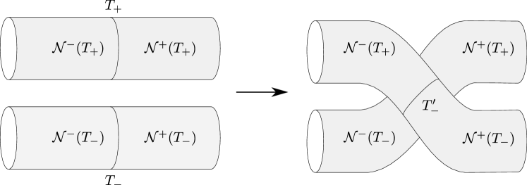
Figure 9. Splicing along tori.

Definition 3.1.

We will say that $(M^{\prime},\xi^{\prime})$ constructed above is the contact manifold obtained from $(M,\xi)$ by splicing along $(T_{+},K_{+})$ and $(T_{-},K_{-})$.

Example 3.2.

Consider the tight contact torus $({\mathbb{T}}^{3},\xi_{n})$ for $n\in{\mathbb{N}}$, where

$$\xi_{n}=\ker\bigl{[}\cos(2\pi n\rho)\,d\vartheta+\sin(2\pi n\rho)\,d\varphi\bigr{]}$$

in coordinates $(\varphi,\vartheta,\rho)\in{\mathbb{T}}^{3}$. Then $T_{0}:=\{\rho=0\}$ is a pre-Lagrangian torus, to which we assign the natural orientation induced by the coordinates $(\varphi,\vartheta)$. If $(M,\xi)$ is another connected contact $3$–manifold with an oriented pre-Lagrangian torus $T\subset M$, then splicing $(M,\xi)\sqcup({\mathbb{T}}^{3},\xi_{n})$ along $T$ and $T_{0}$ produces a new connected contact manifold, namely the one obtained from $(M,\xi)$ by performing $n$ Lutz twists along $T$. If $T\subset M$ is compressible then the resulting contact manifold is overtwisted; by contrast, Lutz twists along incompressible tori can be used to construct tight contact manifolds with arbitrarily large Giroux torsion. Note that in this example the choice of the transverse cycles on $T$ and $T_{0}$ does not influence the resulting manifold.

Remark 3.3.

Note that if $(M,\xi)$ is a contact $3$–manifold with an $\SS^{1}$–action such that the oriented pre-Lagrangian tori $T_{+},T_{-}\subset M$ consist of Legendrian $\SS^{1}$–orbits, then the splicing operation can be assumed compatible with the circle action, in the sense that the manifold $(M^{\prime},\xi^{\prime})$ obtained by splicing is then also an $\SS^{1}$–manifold, with the tori $T_{\pm}^{\prime}$ consisting of Legendrian orbits.

If sections $\sigma_{\pm}$ of the $\SS^{1}$–action are given in a neighborhood of the tori $T_{+},T_{-}$ in $(M,\xi)$, then we can obtain any desired intersection number $e_{+}$ between $\sigma_{-}\cap\mathcal{N}^{-}(T_{-})$ and $\sigma_{+}\cap\mathcal{N}^{+}(T_{+})$ in $T_{+}^{\prime}$ by letting the cycle $K_{-}$ be the intersection $\sigma_{-}\cap T_{-}$, and choosing a cycle $K_{+}$ that has intersection number $e_{+}$ with $\sigma_{+}$. The intersection number $e_{-}$ between $\sigma_{+}\cap\mathcal{N}^{-}(T_{+})$ and $\sigma_{-}\cap\mathcal{N}^{+}(T_{-})$ in $T_{-}^{\prime}$ will always be equal to $-e_{+}$.

Note in particular that we can arrange for the sections $\sigma_{\pm}$ to glue smoothly after splicing by choosing both cycles $K_{\pm}\subset T_{\pm}$ to be the intersections $\sigma_{\pm}\cap T_{\pm}$.

3.2. Attaching handles

Given $\delta>0$, we will use the term toroidal $1$–handle to refer to the smooth manifold with boundary and corners,

$${H}_{\delta}={\mathbb{T}}^{2}\times[-\delta,\delta]\times[-\delta,\delta]\;.$$

Let $(\varphi,\vartheta;r,r^{\prime})$ denote the natural coordinates on ${H}_{\delta}$, and label the smooth pieces of its boundary $\partial{H}_{\delta}=\partial^{N}{H}_{\delta}\cup\partial^{S}{H}_{\delta}\cup\partial^{W}{H}_{\delta}\cup\partial^{E}{H}_{\delta}$ as follows:

$$\partial^{N}{H}_{\delta}=\{r^{\prime}=+\delta\},\qquad\partial^{S}{H}_{\delta}=\{r^{\prime}=-\delta\},\qquad\partial^{W}{H}_{\delta}=\{r=-\delta\},\text{ and }\partial^{E}{H}_{\delta}=\{r=+\delta\}\;.$$

Observe that if we assign the natural boundary orientations to each of these pieces, then the induced coordinates $(\varphi,\vartheta;r)$ are negatively oriented on $\partial^{N}{H}_{\delta}$ but positively oriented on $\partial^{S}{H}_{\delta}$; similarly, the coordinates $(\varphi,\vartheta;r^{\prime})$ are negatively oriented on $\partial^{W}{H}_{\delta}$, and positively oriented on $\partial^{E}{H}_{\delta}$.

Suppose $(M,\xi)$ is a contact manifold, $W=(-\varepsilon,0]\times M$ is a collar neighborhood with $\partial W=M$, and $T_{+},T_{-}\subset M$ are oriented pre-Lagrangian tori with transverse $1$–cycles $K_{\pm}\subset T_{\pm}$ and standard coordinates $(\varphi,\vartheta;r)$ on a pair of disjoint neighborhoods

$${\mathbb{T}}^{2}\times(-\varepsilon,\varepsilon)\cong\mathcal{N}(T_{\pm})\subset M\;.$$

Choosing $\delta$ with $0<\delta<\varepsilon$, we can attach ${H}_{\delta}$ to $W$ along $(T_{+},K_{+})$ and $(T_{-},K_{-})$ via the orientation reversing embeddings

$$\begin{split}\Phi:\,&\partial^{N}{H}_{\delta}\hookrightarrow\mathcal{N}(T_{+}),\,(\varphi,\vartheta;r,\delta)\mapsto(\varphi,\vartheta;r)\\ \Phi:\,&\partial^{S}{H}_{\delta}\hookrightarrow\mathcal{N}(T_{-}),\,(\varphi,\vartheta;r,-\delta)\mapsto(\varphi,\vartheta;-r)\;.\end{split}$$

Then if $W^{\prime}=W\cup_{\Phi}{H}_{\delta}$, after smoothing the corners, the new boundary $M^{\prime}=\partial W^{\prime}$ is diffeomorphic to the manifold obtained from $M$ by splicing along ($T_{+},K_{+})$ and $(T_{-},K_{-})$, where the distinguished tori $T_{\pm}^{\prime}\subset M^{\prime}$ are naturally identified with

$$T_{\pm}^{\prime}={\mathbb{T}}^{2}\times\bigl{\{}(\pm\delta,0)\bigr{\}}\subset\partial^{W}{H}_{\delta}\cup\partial^{E}{H}_{\delta}\subset M^{\prime}\;.$$

The main result of this section is that such an operation can also be defined in the symplectic and contact categories.

Theorem 3.4.

Suppose $(W,\omega)$ is a symplectic manifold with weakly contact boundary $(M,\xi)$, and $T_{+},T_{-}\subset M$ are disjoint, oriented pre-Lagrangian tori with rational linear characteristic foliations and transverse $1$–cycles $K_{\pm}\subset T_{\pm}$, such that $T_{\pm}$ are also symplectic with respect to $\omega$, with

$$\int_{T_{+}}\omega=\int_{T_{-}}\omega>0\;.$$

Then after a symplectic deformation of $\omega$ near $T_{+}\cup T_{-}$, $\omega$ extends to a symplectic form $\omega^{\prime}$ on the manifold

$$W^{\prime}=W\cup{H}_{\delta}$$

obtained by attaching a toroidal $1$–handle ${H}_{\delta}$ to $W$ along $(T_{+},K_{+})$ and $(T_{-},K_{-})$, so that $(W^{\prime},\omega^{\prime})$ then has weakly contact boundary $(M^{\prime},\xi^{\prime})$, where the latter is obtained from $(M,\xi)$ by splicing along $(T_{+},K_{+})$ and $(T_{-},K_{-})$.

As we saw in Example 3.2, Lutz twists along a pre-Lagrangian torus $T\subset(M,\xi)$ can always be realized by splicing $(M,\xi)$ together with a tight contact $3$–torus, and due to the construction of Giroux [Gir94], the latter admits weak fillings for which the pre-Lagrangian tori $\{\rho=\text{const}\}$ are symplectic. Thus whenever $(M,\xi)$ has weak filling $(W,\omega)$ and $T\subset M=\partial W$ is a torus that is both pre-Lagrangian in $(M,\xi)$ and symplectic in $(W,\omega)$, the above theorem can be used to construct weak fillings of every contact manifold obtained by performing finitely many Lutz twists along $T$. We will see however that the setup needed to prove the theorem yields a much more concrete construction of such a filling:

Theorem 3.5.

Suppose $(W,\omega)$ is a symplectic manifold with weakly contact boundary $(M,\xi)$, and $T\subset M$ is a pre-Lagrangian torus which is also symplectic with respect to $\omega$. Then for any $n\in{\mathbb{N}}$, $(W,\omega)$ can be deformed symplectically so that it is also positive on $\xi_{n}$, where the latter is obtained from $\xi$ by performing $n$ Lutz twists along $T$.

To prove both of these results, we begin by constructing a suitable symplectic deformation of a weak filling near any symplectic pre-Lagrangian torus. The local setup is as follows: let

$$M={\mathbb{T}}^{2}\times[-5\varepsilon,5\varepsilon]$$

with coordinates $(\varphi,\vartheta;r)$ and contact structure $\xi=\ker\lambda$, where

$$\lambda=d\vartheta+r\,d\varphi\;.$$

Define also

$$W=(-\varepsilon,0]\times M$$

with coordinates $(t;\varphi,\vartheta;r)$, and identifying $M$ with $\partial W=\{0\}\times M$, assume $\Omega$ is a closed $2$–form on $M$ such that ${\left.{\Omega}\right|_{\xi}}>0$, and

$$\omega=d(t\,\lambda)+\Omega$$

is a symplectic form on $W$. Lemma 2.3 guarantees that $\omega$ can always be put in this form without loss of generality. Moreover, assume $\Omega$ is positive on the torus

$$T:={\mathbb{T}}^{2}\times\{0\}\subset M\;.$$

By shrinking $\varepsilon$ if necessary, we can then assume without loss of generality that $\omega$ is positive on each of the tori $\{t\}\times{\mathbb{T}}^{2}\times\{r\}$ for $t\in(-\varepsilon,0]$ and $r\in[-5\varepsilon,5\varepsilon]$. Define the constant

(3.1) $$A=\int_{T}\omega>0\;.$$

Let us now define a family of $1$–forms on $M$,

$$\lambda_{\sigma}=d\vartheta+g_{\sigma}(r)\,d\varphi$$

for $\sigma\in[0,1]$, where $g_{\sigma}:\,[-5\varepsilon,5\varepsilon]\to{\mathbb{R}}$ is a smooth $1$–parameter family of odd functions such that:

1. $g_{\sigma}(r)=r$, and $g_{\sigma}(0)=0$ for all $\sigma\in[0,1]$ when ${\left\lvert r\right\rvert}\geq 4\varepsilon$,

2. $g_{\sigma}^{\prime}>0$ for all $\sigma\in(0,1]$,

3. $g_{1}(r)=r$ for all $r$,

4. $g_{0}(r)=0$ for all ${\left\lvert r\right\rvert}\leq 3\varepsilon$.

Then $\lambda_{1}=\lambda$, $\lambda_{\sigma}$ is a contact form for all $\sigma\in(0,1]$ and $\lambda_{0}$ defines a confoliation, which is integrable in the region $\bigl{\{}{\left\lvert r\right\rvert}\leq 3\varepsilon\bigr{\}}$. Let $\xi_{\sigma}=\ker\lambda_{\sigma}$. By shrinking $\varepsilon$ again if necessary, we can assume without loss of generality that each $\xi_{\sigma}$ is sufficiently $C^{0}$–close to $\xi$ so that

$${\left.{\Omega}\right|_{\xi_{\sigma}}}>0$$

for all $\sigma\in[0,1]$.

Next, choose a smooth cutoff function

$$\beta:\,[-5\varepsilon,5\varepsilon]\to[0,1]$$

that has support in $[-3\varepsilon,3\varepsilon]$ and is identically $1$ on $[-2\varepsilon,2\varepsilon]$. We use this to define a smooth $2$–parameter family of $1$–forms for $(\sigma,\tau)\in[0,1]\times[0,1]$,

(3.2) $$\lambda_{\sigma}^{\tau}=(1-\tau)\beta(r)\,dr+\bigl{[}1-(1-\tau)\beta(r)\bigr{]}\,\lambda_{\sigma},$$

and distributions $\xi_{\sigma}^{\tau}=\ker\lambda_{\sigma}^{\tau}$. The following lemma implies that $\xi_{\sigma}^{\tau}$ is a contact structure whenever both $\sigma$ and $\tau$ are positive.

Lemma 3.6.

Suppose $f(r)$ and $g(r)$ are any two smooth real valued functions on $[-5\varepsilon,5\varepsilon]$ such that the $1$–form

$$\alpha=f(r)\,d\vartheta+g(r)\,d\varphi$$

on ${\mathbb{T}}^{2}\times[-5\varepsilon,5\varepsilon]$ is contact. Then for any $t\in[0,1)$, the $1$–form

$$\alpha_{t}:=t\beta(r)\,dr+\bigl{[}1-t\beta(r)\bigr{]}\,\alpha$$

is also contact.

Démonstration.

Noting that $dr\wedge d\alpha=0$, we compute

$$\begin{split}\alpha_{t}\wedge d\alpha_{t}&=\bigl{[}t\beta\,dr+(1-t\beta)\,\alpha\bigr{]}\wedge\bigl{[}(1-t\beta)\,d\alpha-t\beta^{\prime}\,dr\wedge\alpha\bigr{]}\\ &=(1-t\beta)^{2}\,\alpha\wedge d\alpha\neq 0\;.\qed\end{split}$$

By Gray’s stability theorem, each of the contact structures $\xi_{\sigma}^{\tau}$ for $\sigma,\tau>0$ are related to $\xi=\xi_{1}^{1}$ by isotopies with support in ${\mathbb{T}}^{2}\times[-4\varepsilon,4\varepsilon]$. Thus after a compactly supported isotopy, we can view $\xi$ as a small perturbation of the confoliation $\bar{\xi}:=\xi_{0}^{0}=\ker\bar{\lambda}$, where we define

$$\bar{\lambda}=\lambda_{0}^{0}=\beta(r)\,dr+\bigl{[}1-\beta(r)\bigr{]}\,\left(d\vartheta+g_{0}(r)\,d\varphi\right)\;.$$

This $1$–form is identical to $\lambda$ in $\bigl{\{}{\left\lvert r\right\rvert}\geq 4\varepsilon\bigr{\}}$, but defines a foliation in $\bigl{\{}{\left\lvert r\right\rvert}\leq 3\varepsilon\bigr{\}}$ and takes the especially simple form

$$\bar{\lambda}=dr\quad\text{in ${\mathbb{T}}^{2}\times[-2\varepsilon,2\varepsilon]$}\;.$$

The main technical ingredient we need is then the following deformation result.

Proposition 3.7.

Given the local model of a symplectic pre-Lagrangian torus $T\subset M=\partial W$ described above, for any sufficiently large constant $C>0$ there exists a symplectic form $\bar{\omega}$ on $W$ with the following properties:

1. $\bar{\omega}=\omega$ outside some compact neighborhood of $T$ in $W$,

2. ${\left.{\bar{\omega}}\right|_{\bar{\xi}}}>0$,

3. $\bar{\omega}=A\,d\varphi\wedge d\vartheta+C\,dt\wedge dr$ on some neighborhood of $T$.

Démonstration.

Note that $\Omega$ restricts on each of the $2$–plane fields $\xi_{\sigma}^{\tau}=\ker\lambda_{\sigma}^{\tau}$ to a positive form. This is clear, because $\lambda_{\sigma}^{\tau}$ as defined in (3.2) is pointwise a convex combination of $dr$ and $\lambda_{\sigma}$, where $\lambda_{\sigma}\wedge\Omega$ and $dr\wedge\Omega$ are both positive, the latter due to the assumption that the tori ${\mathbb{T}}^{2}\times\{r\}$ are all symplectic, the former because $\varepsilon$ was chosen small enough to guarantee that ${\left.{\Omega}\right|_{\xi_{\sigma}}}>0$. We therefore find a smooth homotopy from $\xi$ to $\bar{\xi}$, supported in a neighborhood of $T$, through confoliations on which $\Omega$ is always positive.

Next, let us replace $\Omega$ by a cohomologous closed $2$–form that takes a much simpler form near $T$. Indeed, since $\int_{T}\Omega=A=\int_{T}A\,d\varphi\wedge d\vartheta$ and $T$ generates $H_{2}(M)$, there exists a $1$–form $\eta$ on $M$ such that

$$A\,d\varphi\wedge d\vartheta=\Omega+d\eta\;.$$

Choose a smooth cutoff function $F:[-5\varepsilon,5\varepsilon]\to[0,1]$ that has compact support in $[-2\varepsilon,2\varepsilon]$ and equals $1$ on $[-\varepsilon,\varepsilon]$, and define the closed $2$–form

$$\bar{\Omega}=\Omega+d(F(r)\,\eta)\;,$$

which equals $\Omega$ outside of $\bigl{\{}{\left\lvert r\right\rvert}\leq 2\varepsilon\bigr{\}}$ and $A\,d\varphi\wedge d\vartheta$ in $\bigl{\{}{\left\lvert r\right\rvert}\leq\varepsilon\bigr{\}}$. We claim

$${\left.{\bar{\Omega}}\right|_{\bar{\xi}}}>0\;.$$

Indeed, outside of the region $\bigl{\{}{\left\lvert r\right\rvert}\leq 2\varepsilon\bigr{\}}$ this statement is nothing new, and otherwise $\bar{\lambda}=dr$, so we compute

$$\bar{\lambda}\wedge\bar{\Omega}=dr\wedge\bigl{[}(1-F(r))\,\Omega+AF(r)\,d\varphi\wedge d\vartheta\bigr{]}>0\;.$$

The result now follows by applying Lemmas 2.11 and 2.10, in that order. This deforms $\omega$ near $T$ to a symplectic structure of the form

$$\bar{\omega}=d(\varphi\,\bar{\lambda})+\bar{\Omega}\;,$$

where $\varphi(t;\varphi,\vartheta;r)$ depends only on $t$ near $T$ and satisfies $\partial_{t}\varphi>0$, so plugging in the local formulas $\bar{\lambda}=dr$ and $\bar{\Omega}=A\,d\varphi\wedge d\vartheta$, the above becomes

$$\bar{\omega}=\partial_{t}\varphi\,dt\wedge dr+A\,d\varphi\wedge d\vartheta\;.$$

One can also easily arrange for $\partial_{t}\varphi$ to be constant near $T$ so long as it is sufficiently large, and the result is thus proved. ∎

Proof of Theorem 3.5.

The following argument generalizes the construction of weak fillings on tight $3$–tori described by Giroux [Gir94]. Consider the confoliation $\bar{\xi}$ and deformed symplectic structure $\bar{\omega}$ constructed in Proposition 3.7. Then $\bar{\omega}$ is also positive on any contact structure $\xi^{\prime}$ that is sufficiently $C^{0}$–close to $\bar{\xi}$ as a distribution. It suffices therefore to find, for any $n\in{\mathbb{N}}$, a contact structure $\xi_{n}$ that is $C^{0}$–close to $\bar{\xi}$ and isotopic to the one obtained by performing $n$ Lutz twists on $\xi$ along $T$. This is easy: for $\sigma\in[0,1]$, define a smooth family of confoliation $1$–forms $\alpha_{\sigma}$ which match $\lambda_{\sigma}$ outside the coordinate neighborhood ${\mathbb{T}}^{2}\times[-\varepsilon,\varepsilon]$, and in ${\mathbb{T}}^{2}\times[-\varepsilon,\varepsilon]$ are contact and take the form

$$F_{\sigma}(r)\,d\vartheta+G_{\sigma}(r)\,d\varphi\;,$$

such that the curve $r\mapsto(F_{0}(r),G_{0}(r))\in{\mathbb{R}}^{2}$ winds $n$ times counterclockwise about the origin for $r\in[-\varepsilon,\varepsilon]$. Then $\alpha_{\sigma}$ is contact for every $\sigma\in(0,1]$ and defines a contact structure isotopic to the one we are interested in. It follows now from Lemma 3.6 that for all $\sigma\in(0,1]$ and $\tau\in(0,1]$,

$$\alpha_{\sigma}^{\tau}:=(1-\tau)\beta(r)\,dr+\left[1-(1-\tau)\beta(r)\right]\alpha_{\sigma}$$

is a contact form, but as $\sigma\to 0$ and $\tau\to 0$ it converges to $\bar{\lambda}$. ∎

Proof of Theorem 3.4.

We assume $(W,\omega)$ is a symplectic manifold with weakly contact boundary $(M,\xi)$, and $T_{+},T_{-}\subset M\subset W$ are oriented tori which are pre-Lagrangian in $(M,\xi)$ and symplectic in $(W,\omega)$, such that

$$\int_{T_{-}}\omega=\int_{T_{+}}\omega=A>0\;.$$

Then for a sufficiently large constant $C>0$, we can use Proposition 3.7 to deform $\omega$ near $T_{+}$ and $T_{-}$ to a new symplectic structure $\bar{\omega}$, which takes the form

$$\bar{\omega}=C\,dt\wedge dr+A\,d\varphi\wedge d\vartheta$$

in local coordinates near $T_{+}$ and $T_{-}$, and satisfies ${\left.{\bar{\omega}}\right|_{\bar{\xi}}}>0$. Here $\bar{\xi}$ is a confoliation with the following properties:

• $\bar{\xi}=\xi$ outside a small coordinate neighborhood $N\subset M$ of $T_{+}\cup T_{-}$,

• $\bar{\xi}$ admits a $C^{0}$–small perturbation to a contact structure, which is isotopic to $\xi$ by an isotopy supported in $N$,

• $\bar{\xi}=\ker dr$ on an even smaller coordinate neighborhood of $T_{+}\cup T_{-}$.

Choose $\delta>0$ sufficiently small so that the coordinate neighborhoods ${\mathbb{T}}^{2}\times[-\delta,\delta]$ of $T_{-}$ and $T_{+}$ are contained in the region where $\bar{\xi}=\ker dr$ and $\bar{\omega}=C\,dt\wedge dr+A\,d\varphi\wedge d\vartheta$. Then we define the following smooth model of a toroidal $1$–handle (see Figure 10):

$${H}_{\delta}=\Bigl{\{}(\varphi,\vartheta;r,r^{\prime})\in{\mathbb{T}}^{2}\times[-\delta,\delta]\times[-\delta,\delta]\,\Bigm{|}\ {\left\lvert r\right\rvert}\leq h(r^{\prime})\Bigr{\}}\;,$$

where $h:\,[-\delta,\delta]\to(0,\delta]$ is a continuous, even and convex function that is smooth on $(-\delta,\delta)$ and has its derivative blowing up at $r^{\prime}=\pm\delta$, such that its graph merges smoothly into the lines $r^{\prime}=\pm\delta$. Denote the smooth pieces of $\partial{H}_{\delta}$ by

$$\partial^{N}{H}_{\delta}=\{r^{\prime}=+\delta\},\,\partial^{S}{H}_{\delta}=\{r^{\prime}=-\delta\},\,\partial^{W}{H}_{\delta}=\{r=-h(r^{\prime})\},\,\text{ and }\,\partial^{E}{H}_{\delta}=\{r=+h(r^{\prime})\}\;.$$

This model can be attached smoothly to $W$ as in Figure 10, so that

$$W^{\prime}:=W\cup{H}_{\delta}$$

has smooth boundary $M^{\prime}:=\partial W^{\prime}$. The symplectic structure $\bar{\omega}$ then extends to $W^{\prime}$ by defining

$$\bar{\omega}=C\,dr^{\prime}\wedge dr+A\,d\varphi\wedge d\vartheta$$

on ${H}_{\delta}$, which restricts positively to the smooth confoliation $\bar{\xi}^{\prime}$ on $M^{\prime}$ defined by

$$\bar{\xi}^{\prime}=\begin{cases}\bar{\xi}&\text{ on $M\setminus(\partial^{N}{H}_{\delta}\cup\partial^{S}{H}_{\delta})$,}\\ T({\mathbb{T}}^{2}\times\{*\})&\text{ on $\partial^{W}{H}_{\delta}\cup\partial^{E}{H}_{\delta}$.}\end{cases}$$

The latter admits a $C^{0}$–small perturbation to a contact form which is isotopic to the one obtained by splicing $(M,\xi)$ along $T_{+}$ and $T_{-}$. ∎

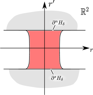
Figure 10. The handle ${H}_{\delta}$ is attached in the ambient space ${\mathbb{T}}^{2}\times{\mathbb{R}}^{2}$ to two model neighborhoods.

3.3. Proof of Theorem 5

Assume $\Sigma=\Sigma_{+}\cup_{\Gamma}\Sigma_{-}$ is a closed oriented surface that is the union of two surfaces with boundary along a multicurve $\Gamma\subset\Sigma$ whose connected components are all nonseparating, and let $\bigl{(}P_{\Sigma,e},\xi_{\Gamma,e}\bigr{)}$ denote the $\SS^{1}$–principal bundle $P_{\Sigma,e}$ over $\Sigma$ with Euler number $e$ together with the $\SS^{1}$–invariant contact structure $\xi_{\Gamma,e}$ that is everywhere transverse to the $\SS^{1}$–fibers with exception of the tori that lie over the multicurve $\Gamma$. Under these assumptions, we will use the handle attaching technique described in §3.2 to construct a weak filling of $\bigl{(}P_{\Sigma,e},\xi_{\Gamma,e}\bigr{)}$. The idea is to obtain $\bigl{(}P_{\Sigma,e},\xi_{\Gamma,e}\bigr{)}$ by a sequence of splicing operations from a simpler disconnected contact manifold for which a (disconnected) strong filling is easy to construct by hand. For this strong filling, the components of $\Gamma$ give rise to pre-Lagrangian tori, and the significance of the nonseparating assumption will be that it allows us to perturb the strong filling to a weak one for which these tori become symplectic, and are thus suitable for handle attaching.

The building blocks are obtained in the following way. Let $S$ be a connected, oriented compact surface with non-empty boundary. The symmetric double of $S$ is the closed surface

$$S^{D}:=S\cup_{\partial S}\overline{S}\;,$$

where $\overline{S}$ is a second copy of $S$ taken with reversed orientation, and the two are glued along their boundaries via the identity map. The multicurve $\Gamma_{S}:=\partial S\subset S^{D}$ determines an $\SS^{1}$–invariant contact manifold $(\SS^{1}\times S^{D},\xi_{\Gamma_{S}})$ in the standard way.

Proposition 3.8.

The contact manifold $(\SS^{1}\times S^{D},\xi_{\Gamma_{S}})$ obtained from a symmetric double has a strong symplectic filling homeomorphic to $[0,1]\times\SS^{1}\times S$.

Démonstration.

Regard $S$ together with a positive volume form $\Omega_{S}$ as a symplectic manifold. Choose a plurisubharmonic Morse function $f:\,S\to[0,C]$ whose critical values all lie in the interval $[0,\varepsilon]$ with $\varepsilon<C$, such that $f^{-1}(C)=\partial S$. Take now the annulus ${\mathbb{R}}\times\SS^{1}$ with symplectic form $dx\wedge d\varphi$, and with plurisubharmonic function $g(x,\varphi)=x^{2}$. The product manifold

$$\bigl{(}({\mathbb{R}}\times\SS^{1})\times S,\Omega+dx\wedge d\varphi\bigr{)}$$

is a symplectic manifold with a plurisubharmonic function given by $F:=f+x^{2}$. The critical values of this function all lie in $[0,\varepsilon]$, so that $N:=F^{-1}(C)$ will be a smooth compact hypersurface. In fact, it is easy to see that $N$ is diffeomorphic to $\SS^{1}\times S^{D}$. The standard circle action on the annulus ${\mathbb{R}}\times\SS^{1}$ splits off naturally, so that $N$ is the product of a circle with a closed surface.

We can explicitly give two embeddings of the $3$–manifold $\SS^{1}\times S$ into $F^{-1}(C)\subset({\mathbb{R}}\times\SS^{1})\times S$ as the graphs of the two maps $\SS^{1}\times S\to({\mathbb{R}}\times\SS^{1})\times S,\,(\varphi,p)\mapsto\bigl{(}\pm\sqrt{C-f(p)},\varphi,p\bigr{)}$ distinguished by the different signs in front of the square root. The boundary of $\SS^{1}\times S$ is mapped by both maps to the set $\{0\}\times\SS^{1}\times\partial S$ so that the two copies are glued along their boundary.

The contact form is defined as $\alpha:=-{\left.{d^{c}F}\right|_{TN}}=-{\left.{dF\circ J}\right|_{TN}}$. It is $\SS^{1}$–invariant (for the standard complex structure on ${\mathbb{R}}\times\SS^{1}$), and the vector $\partial_{\varphi}$ is parallel to $N$, and never lies in the kernel of $\alpha$ with the exception of the points where $d(x^{2})$ vanishes, which happens to be exactly along the boundary of $S$. By [Lut77], this proves that the hypersurface $N$ is contactomorphic to $(\SS^{1}\times S^{D},\xi_{\Gamma_{S}})$. ∎

Now denote by

$$\Sigma_{1},\dotsc,\Sigma_{N}$$

the closures of the connected components of $\Sigma\setminus\Gamma$, whose boundaries $\Gamma_{j}:=\partial\Sigma_{j}$ are all disconnected due to the assumption that components of $\Gamma$ are nonseparating. Then for each $j=1,\dotsc,N$, construct the doubled manifold $\Sigma_{j}^{D}$, and define the disconnected contact manifold

$$(M_{0},\xi_{0})=\bigsqcup_{j=1}^{N}(\SS^{1}\times\Sigma_{j}^{D},\xi_{\Gamma_{j}})\;,$$

which by the proposition above can be strongly filled. Let $(W_{j},\omega_{j})$ denote the resulting strong filling of $\SS^{1}\times\Sigma_{j}^{D}$. For each connected component $\gamma\subset\Gamma_{j}$, which is also a component of $\Gamma$, the torus $\SS^{1}\times\gamma\subset\partial W_{j}$ is a Lagrangian submanifold in $(W_{j},\omega_{j})$.

Lemma 3.9.

There exists a cohomology class $[\beta]\in H^{2}_{\operatorname{dR}}\bigl{(}P_{\Sigma,e}\bigr{)}$ such that $\int_{T}\beta\neq 0$ for every torus $T$ that lies over a connected component $\gamma\subset\Gamma$.

Démonstration.

By Poincaré duality, it suffices to find a homology class $A\in H_{1}\bigl{(}P_{\Sigma,e};{\mathbb{R}}\bigr{)}$ whose intersection number $A\bullet[T_{\gamma}]\in{\mathbb{R}}$ is nonzero for every torus $T_{\gamma}$ lying over a connected component $\gamma\subset\Gamma$. For each component $\gamma\in\Gamma$, pick an oriented loop $C_{\gamma}$ in $P_{\Sigma,e}$ with $[C_{\gamma}]\bullet[T_{\gamma}]=1$; this necessarily exists since $\gamma$ and hence also $T_{\gamma}$ is nonseparating. Then we construct $A$ by the following algorithm: starting with any connected component $\gamma_{1}\subset\Gamma$, let $A_{1}=[C_{\gamma_{1}}]$. Then $A_{1}\bullet[T_{\gamma}]\neq 0$ for some subcollection of the components $\gamma\subset\Gamma$, including $\gamma_{1}$. If there remains a component $\gamma_{2}\subset\Gamma$ such that $A_{1}\bullet[T_{\gamma_{2}}]=0$, then we set

$$A_{2}=A_{1}+d_{2}\,[C_{\gamma_{2}}]\;,$$

where $d_{2}>0$ is chosen sufficiently small so that for every component $\gamma\subset\Gamma$ with $A_{1}\bullet[T_{\gamma}]$ nonzero, $A_{2}\bullet[T_{\gamma}]$ is also nonzero. The result is that $A_{2}\bullet[T_{\gamma}]$ is nonzero for a strictly larger set of components than $A_{1}\bullet[T_{\gamma}]$. Thus after repeating this process finitely many times, we eventually find $A\in H_{1}\bigl{(}P_{\Sigma,e};{\mathbb{R}}\bigr{)}$ with all intersection numbers $A\bullet[T_{\gamma}]$ nonzero. ∎

Using the cohomology class $[\beta]$ given by the lemma, orient every torus $T_{\gamma}\subset P_{\Sigma,e}$ that projects onto a connected component $\gamma\subset\Gamma$ in such a way that $\int_{T_{\gamma}}\beta>0$. We find a closed $2$–form $\sigma$ representing $[\beta]$ that is positive on each of the oriented pre-Lagrangian tori $T_{\gamma}$. Since every component $\Sigma_{j}$ has non-empty boundary, it follows that the restriction ${\left.{P_{\Sigma,e}}\right|_{\Sigma_{j}}}$ is trivial so that we can identify it with

$${\left.{P_{\Sigma,e}}\right|_{\Sigma_{j}}}\cong\SS^{1}\times\Sigma_{j}\;,$$

and we can then pull-back $\sigma$ to each component $\SS^{1}\times\Sigma_{j}$ to obtain a collection of $2$–forms $\sigma_{j}$ on the fillings $W_{j}\cong[0,1]\times\SS^{1}\times\Sigma_{j}$, all of which are positive on the tori $\SS^{1}\times\gamma\subset W_{j}$. The same is then true for the $2$–forms $\omega_{j}+\varepsilon\,\sigma_{j}$, with $\varepsilon>0$ chosen sufficiently small so that

$$(W_{0},\omega_{0}):=\bigsqcup_{j=1}^{N}(W_{j},\omega_{j}+\varepsilon\,\sigma_{j})$$

is a weak filling of $(M_{0},\xi_{0})$.

Observe now that each torus $T_{\gamma}$ for a connected component $\gamma\subset\Gamma$ corresponds to two pre-Lagrangian tori in $(M_{0},\xi_{0})$, which are symplectic in $(W_{0},\omega_{0})$ and have matching integrals of $\omega_{0}$ by construction. This allows us to attach toroidal $1$–handles to $(W_{0},\omega_{0})$ along corresponding pairs of tori via Theorem 3.4, which by Remark 3.3 can be done in a way that is compatible with circle actions. To prescribe the isotopy class of the gluing maps, choose for all except one of the tori $T_{\gamma}\subset M_{0}$ the curves $\{*\}\times\partial\Sigma_{j}$ as the transverse cycle. This way the splicing will glue the sections $\{*\}\times\Sigma_{j}$ together smoothly along each of the pre-Lagrangian tori. If the transverse cycle is also chosen to be of the form $\{*\}\times\partial\Sigma_{j}$ on the last torus, then the section will in fact glue to a global section, and the resulting manifold will be a weak filling of two disjoint copies of the contact manifold $(\SS^{1}\times\Sigma,\xi_{\Gamma})$. If we instead choose a different transverse cycle on the last torus, we obtain a connected symplectic manifold with weak contact boundary consisting of the disjoint union of the circle bundles $\bigl{(}P_{\Sigma,e},\xi_{\Gamma,e}\bigr{)}$ and $\bigl{(}P_{\Sigma,-e},\xi_{\Gamma,-e}\bigr{)}$ with the corresponding contact structures. We claim that the Euler number $e$ is given by the intersection number of the two sections touching the last pre-Lagrangian torus $T_{0}$, which is equal to the intersection number of the chosen transverse cycle with the curve $\{*\}\times\partial\Sigma_{j}$ . The Euler number is obtained by chosing a section over a disk $D$, a section over the complement of this disk, and computing the intersection number of both sections in the torus that lies over the boundary $\partial D$. Our construction yields so far a section of the spliced manifold defined everywhere except at the last pre-Lagrangian torus $T_{0}$. We can push both parts of the section a bit away from $T_{0}$, and connect them with a strip crossing this torus. The new section obtained this way is defined over the whole surface $\Sigma$ with the exception of a disk $D$, and it is easy to see that the intersection number between the section we have just constructed, and a section over $D$ is equal to the intersection number of the two initial sections in the pre-Lagrangian torus $T_{0}$.

Finally, capping the weak contact boundary $\bigl{(}P_{\Sigma,-e},\xi_{\Gamma,-e}\bigr{)}$ using [Eli04, Etn04a], we obtain a weak filling of $\bigl{(}P_{\Sigma,e},\xi_{\Gamma,e}\bigr{)}$, thus the proof of Theorem 5 is complete.