On the role of Allee effect and mass migration in survival and extinction of a species

Abstract

We use interacting particle systems to investigate survival and extinction of a species with colonies located on each site of $\mathbb{Z}^{d}$. In each of the four models studied, an individual in a local population can reproduce, die or migrate to neighboring sites.

We prove that an increase of the death rate when the local population density is small (the Allee effect) may be critical for survival, and that the migration of large flocks of individuals is a possible solution to avoid extinction when the Allee effect is strong. We use attractiveness and comparison with oriented percolation, either to prove the extinction of the species, or to construct nontrivial invariant measures for each model.

T1Supported by Fondation Sciences Mathématiques de Paris. T2Supported by the French Ministry of Education through the Grant ANR BLAN07-218426.

1 Introduction

A metapopulation model refers to many small local populations connected via migrations in a fragmented environment. Each local population evolves without spatial structure; it can increase or decrease, survive, get extinct or migrate from its site in different ways; see cfHanski for more about metapopulations.

The most natural model for the evolution of a single population is the branching process; see cfGaltonWatts : birth and death rates depend on the number of individuals of the population, and the growth rate is density dependent.

If the birth rate is always larger than the death rate, if the population survives, it will increase indefinitely. If the birth rate is smaller than or equal to the death rate, the population will become extinct almost surely cfWilliams . A more interesting situation is given by a birth rate larger than the death rate under a particular population size $N$, and smaller over that. The real environments observation suggests that this process is gradual; that is, the growth rate decreases over a population size as population density increases. In some of our applications we suppose that over a fixed number of individuals $N$ (the capacity of a site), the growth rate is null.

Many biological phenomena may influence the dynamics of a metapopulation.

Migration is one of the most important strategies that a species adopts to improve its probability of survival (see, e.g., cfBrassil , cfHanski , cfalleestephens ) when the population size is large one or more individuals leave the site where they are located to look for new resources in different sites.

Other biological factors may favor the extinction of a species. One of them, the Allee effect, consists of an increase in the death rate when the density of individuals is small. The reason is that at low density many factors (as difficulties in finding mates) cause a decrease of fecundity and an increase of mortality; see cfallee1 , Allee1 , Allee4 , cfalleestephens .

We simplify the real structure, and we treat $4$ metapopulation models from a mathematical point of view: we start from the easier one by adding a new biological phenomenon at each model.

The mathematical models are interacting particle systems on $\Omega=X^{\mathbb{Z}^{d}}$, where $X\subseteq\mathbb{N}$: each particle represents one individual and on each site of $\mathbb{Z}^{d}$ there is a local population with capacity $N$ (possibly $N=\infty$), which evolves in different ways depending on the model. The local populations are connected via migrations of individuals, that is, jumps of particles from a site to another one.

In Section 2 we introduce the particle system, give the main definitions and notation and state the attractiveness results, crucial in the sequel for the existence of critical parameters and nontrivial invariant measures. Theorem 2.1, the main result of a previous paper (cfBorrello , Theorem 2.4, inspired by GobronSaada ), gives necessary and sufficient conditions for attractiveness of a large class of particle systems. This simplifies many proofs, since, in order to derive either, if two processes are stochastically ordered, or if a process is attractive, we do not need to construct an explicit coupling for each model, but we only have to check inequalities involving the transition rates.

In cfschiallee and cfschiaggr , the author considers a metapopulation model to investigate the roles of mass death (i.e., the death of all individuals in a local population) and spatial aggregation in the extinction of a species. In cfschiallee he shows that, in presence of mass death, animals living in large flocks are more susceptible to extinction than animals living in small flocks: for this model, mass death can be an alternative to the Allee effect in raising to the extinction of a species. The new results in cfschiaggr involve the role of spatial aggregation, which may be either bad or good for survival in a model respectively, with or without mass death. For these models the local population Allee effect was not taken into account. The model introduced, called a noncatastrophic times model, is the following: for a fixed $N<\infty$, on each site of $\mathbb{Z}^{d}$ we may have up to $N$ individuals; hence $N$ is the capacity of sites. The transitions of the Markov process $(\eta_{t})_{t\geq 0}$ are

$$\eta_{t}(x) \to \eta_{t}(x)+1\qquad\mbox{at rate }\eta_{t}(x)\varphi+\lambda\sum_{y\sim x}\mathbh{1}_{\{\eta_{t}(y)=N\}}\mbox{ for }0\leq\eta_{t}(x)<N,$$

$$\eta_{t}(x) \to \eta_{t}(x)-1\qquad\mbox{at rate }1\mbox{ for }1\leq\eta_{t}(x)\leq N,$$

where $y\sim x$ are neighbors. In other words, each individual gives birth to another one on the same site with rate $\varphi$ and dies with rate $1$. An individual on site $x$ gives birth to a new individual in a neighboring site with rate $\lambda/N$ only when the population at $x$ has reached the maximal size $N$. There is a critical parameter for the capacity $N$ of sites:

Theorem 1.1 ((cfschiaggr , Theorem 2))

Assume that $d\geq 2$, $\lambda>0$ and $\varphi>0$. There is a critical value $N_{c}(\lambda,\varphi)$ such that if $N>N_{c}(\lambda,\varphi)$, then starting from any finite number of individuals, the population has a strictly positive probability of surviving.

Starting from noncatastrophic times model, we propose $4$ models to improve the understanding of species dynamics. We want to investigate, for the first time in a model with spatial structure, the role of the Allee effect, the role of mass migration and their interactions.

In Section 3 we introduce Model I. This will represent our basic model with neither Allee effect nor mass migration. We begin with a system very similar to Schinazi’s model: since a further step consists in adding migration of many individuals, we consider a migration of one individual to a neighboring site instead of a birth of a new individual. If $N=1$, such a difference does not allow survival for the model with migrations, since no new births are possible, and the process gets extinct for any $\lambda$: this is definitely not the case for the noncatastrophic times model with $N=1$, which is the contact process. If $N$ is large this small difference does not change the behavior of the model.

This is the basic model, and it must be as easy as possible (births and deaths on the same site and migrations from one site to another, all for at most one particle at time). For this reason we do not consider mass death, which is an additional complex factor.

We take the birth rate larger than the death rate, but we fix a capacity $N$ per site. A migration of one individual from a site $x$ toward a nearest neighbor one, is allowed only when the population on $x$ reaches $N$. We prove that in some cases there is almost sure extinction, and in others the species survives with positive probability: the key tool to prove survival is the comparison technique with a supercritical oriented percolation model; see cfdurrettten .

In Section 4 we introduce Model II, that points out the key role of the Allee effect in species dynamics. Schinazi used mass death to prove that it can be considered an alternative to the Alle effect for extinction of a species. Since both the Allee effect and mass death improve the probability of extinction, in order to understand the role of one of them they should be considered separately. Here we want to show that a strong Allee effect (with neither mass death nor mass migration) is a key factor for the extinction.

We add the Allee effect to Model I. Different probabilistic tools have already been used to illustrate the Allee effect, like stochastic differential equations (see Dennis1 ), discrete-time Markov chains (see Allen ) or diffusion processes (see Dennis2 ), but none of these models has a spatial structure.

In Model II each site has a capacity $N$, but the death rate is larger than the birth rate for small densities. Migration works exactly as in Model I. Theorem 4.1 states that for all possible capacities, growth and migration rates, there exists an Allee effect large enough for the species to become extinct. It is proved through comparison with subcritical percolation.

In Model III, introduced in Section 5, we allow a migration of more than one individual at a time from one site to the neighboring one in a species affected by the Allee effect. We prove that mass migration might be the possible strategy of a species to reduce the Allee effect and improve its survival probability.

When a local population size reaches $N$, a migration of a number of individual smaller than a fixed $M$ is possible. In Model II, for an Allee effect large enough, the species gets extinct. In Model III, if $N$ is large enough there exists $M$ such that this is no longer true. A migration of large flocks avoids small densities in a new environment which are bad for survival. Indeed, by comparison arguments with oriented percolation, even if the Allee effect is the strongest one, if the species lives and migrates in flocks large enough, survival is possible (Theorem 5.1).

In Section 6 we generalize the previous models: in Model IV, instead of fixing a capacity $N$, we consider a slightly more realistic model. In all environments there is no maximal size, but a kind of self-mechanism of birth control such that the death rate is larger than the birth rate when there are more than $N$ individuals in a local population. A migration of one or more individuals is allowed from a site with more than $N$ individuals toward a site with few individuals. We prove in Theorem 6.1 that in some cases we can have survival but on each site the population does not explode even if there is no capacity. Namely, on each site the expected value of the number of individuals is finite. In other cases the species becomes extinct.

Note that on each model instead of fixing the death rate equal to 1 and letting the birth rate vary (the most used approach), we consider the reverse but equivalent point of view in order to clarify our proofs, presented in Section 7.

2 Background and tools

The mathematical model is an interacting particle system $(\eta_{t})_{t\geq 0}$ on $\Omega=X^{\mathbb{Z}^{d}}$, where $X=\{0,1,\ldots,N\}\subseteq\mathbb{N}$ and $N$ denotes the common size (capacity) of the local populations, if finite. The value $\eta_{t}(x)$, $x\in\mathbb{Z}^{d}$, is the number of individuals present in site $x$ at time $t\geq 0$. We write $\Omega_{N}$ when we want to stress the dependency on the capacity $N$.

When $X$ is finite, which is the case of Models I, II and III, we refer to the construction in cfLiggett ; when $X$ is infinite, that is, in Model IV, the state space is noncompact, and a different construction is needed. The first examples of interacting particle systems with locally interacting components in noncompact state spaces have been introduced in Spitzer . One approach to construct these kinds of models has been developed in cfLigSpitz , where the construction was detailed for Coupled Random Walks, but with small changes it can be generalized to many other processes. By using similar ideas, in cfChenbook was stated a general existence theorem for reaction-diffusion processes, that we are going to apply in Model IV: in order to assure the existence of the process, some restrictions on the transition rates are required, as explained in Section 6.

The process admits an invariant measure $\mu$ if $P_{\mu}(\eta_{t}\in A)=\mu(A)$ for each $t\geq 0$, $A\subseteq\Omega$, where $P_{\mu}$ is the law of the process with initial distribution $\mu$. An invariant measure is trivial if it is concentrated on an absorbing state, when one exists. The process is ergodic if there is a unique invariant measure to which the process converges starting from each initial distribution (see cfLiggett , Definition 1.9). For any $x,y\in\mathbb{Z}^{d}$, we write $y\sim x$ if $y$ is one of the $2d$ nearest neighbors of site $x$.

We introduce here a common infinitesimal generator $\mathcal{L}$ (we will be more precise on each model): it is given by

$$\qquad\mathcal{L}f(\eta) = \sum_{x\in\mathbb{Z}^{d}}\sum_{k\in X}\biggl{\{}P^{k}_{\eta(x)}\bigl{(}f(S^{k}_{x}\eta)-f(\eta)\bigr{)}+P^{-k}_{\eta(x)}\bigl{(}f(S^{-k}_{x}\eta(x))-f(\eta)\bigr{)}$$

$$\hskip 98.0pt{}+\sum_{y\sim x}\frac{1}{2d}\Gamma^{k}_{\eta(x),\eta(y)}\bigl{(}f(S^{-k,k}_{x,y}\eta)-f(\eta)\bigr{)}\biggr{\}},$$

where $f$ is a local function, $\eta\in\Omega$, $S^{-k,k}_{x,y}$, $S^{k}_{y}$ and $S^{-k}_{y}$, where $k>0$, are local operators performing the transformations whenever possible

$$(S^{-k,k}_{x,y}\eta)(z) = \cases{\eta(x)-k,&\quad$\mbox{if }z=x\mbox{ and }\eta(x)-k\in X,\eta(y)+k\in X,$\vspace*{2pt}\cr\eta(y)+k,&\quad$\mbox{if }z=y\mbox{ and }\eta(x)-k\in X,\eta(y)+k\in X,$\vspace*{2pt}\cr\eta(z),&\quad$\mbox{otherwise},$}$$ (2)

$$(S^{k}_{y}\eta)(z) = \cases{\eta(y)+k,&\quad$\mbox{if }z=y\mbox{ and }\eta(y)+k\in X,$\vspace*{2pt}\cr\eta(z),&\quad$\mbox{otherwise},$}$$ (3)

$$(S^{-k}_{y}\eta)(z) = \cases{\eta(y)-k,&\quad$\mbox{if }z=y\mbox{ and }\eta(y)-k\in X,$\vspace*{2pt}\cr\eta(z),&\quad$\mbox{otherwise},$}$$ (4)

$P^{k}_{\cdot}$, $P^{-k}_{\cdot}$ are positive functions from $X$ to $\mathbb{R}$, and in our four models $k=0,1$ (particles are born and die one at a time).

We assume $P^{1}_{0}=0$, that is, the Dirac measure concentrated on the empty configuration $\delta_{\underline{0}}$ is a trivial invariant measure. The function $\Gamma^{k}_{\eta(x),\eta(y)}$ represents the migration (jump) rate; a jump of more than one particle per time is possible. We call emigration from $x$ a jump that reduces the number of particles on $x$ and immigration a jump that increases it.

There is a natural definition of partial order on the state space,

$$\forall\xi,\eta\in\Omega,\qquad\xi\leq\eta\quad\Leftrightarrow\quad\bigl{(}\forall x\in S,\xi(x)\leq\eta(x)\bigr{)}.$$ (5)

A process $(\eta_{t})_{t\geq 0}$ with generator $\mathcal{L}$ is stochastically larger than a process $(\xi_{t})_{t\geq 0}$ with generator $\widetilde{\mathcal{L}}$ if, given $\xi_{0}\leq\eta_{0}$, there exists an increasing Markovian coupling $(\xi_{t},\eta_{t})_{t\geq 0}$ on state space $\Omega\times\Omega$ such that

$$\mathbb{P}^{(\xi_{0},\eta_{0})}(\xi_{t}\leq\eta_{t})=1,$$

for all $t\geq 0$, where $\mathbb{P}^{(\xi_{0},\eta_{0})}$ denotes the distribution of $(\xi_{t},\eta_{t})_{t\geq 0}$ with initial state $(\xi_{0},\eta_{0})$. In this case the process $(\xi_{t})_{t\geq 0}$ is stochastically smaller than $(\eta_{t})_{t\geq 0}$, and the pair $(\xi_{t},\eta_{t})_{t\geq 0}$ is stochastically ordered; see cfBorrello , Section 2. If $\mathcal{L}=\widetilde{\mathcal{L}}$, and there is stochastic order between two processes with ordered initial configurations, then the process is attractive; see cfLiggett , Definition II.2.2.

Necessary and sufficient conditions for stochastic order and attractiveness in a general class of particle systems including the models defined by generator (2) have been derived by cfBorrello , Theorem 2.4, which generalizes GobronSaada , Theorem 2.21. Since (2) involves neither births nor deaths depending on neighboring sites, this theorem can be restated as follows:

Theorem 2.1 ((cfBorrello , Theorem 2.4))

Given $K\in\mathbb{N}$, $\mathbf{j}:=\{j_{i}\}_{1\leq i\leq K}$, $\mathbf{m}:=\{m_{i}\}_{1\leq i\leq K}$, $\mathbf{h}:=\{h_{i}\}_{1\leq i\leq K}$, three nondecreasing $K$-uples in $\mathbb{N}$, and $\alpha,\beta,\gamma,\delta$ in $X$ such that $\alpha\leq\gamma$, $\beta\leq\delta$, we define

$$I_{a} := I^{K}_{a}(\mathbf{j},\mathbf{m})=\bigcup^{K}_{i=1}\{k\in X\dvtx m_{i}\geq k>\delta-\beta+j_{i}\},$$ (6)

$$I_{b} := I^{K}_{b}(\mathbf{j},\mathbf{m})=\bigcup^{K}_{i=1}\{k\in X\dvtx\gamma-\alpha+m_{i}\geq k>j_{i}\},$$ (7)

$$I_{c} := I^{K}_{c}(\mathbf{h},\mathbf{m})=\bigcup^{K}_{i=1}\{k\in X\dvtx m_{i}\geq k>\gamma-\alpha+h_{i}\},$$ (8)

$$I_{d} := I^{K}_{d}(\mathbf{h},\mathbf{m})=\bigcup^{K}_{i=1}\{k\in X\dvtx\delta-\beta+m_{i}\geq k>h_{i}\}.$$ (9)

A particle system $(\eta_{t})_{t\geq 0}$ with transition rates $\{\Gamma^{k}_{a,b},P^{k}_{b},P^{-k}_{a}\}_{\{a,b,k\in X\}}$ is stochastically larger than a particle system $(\xi_{t})_{t\geq 0}$ with transition rates $\{\widetilde{\Gamma}^{k}_{a,b},\allowbreak\widetilde{P}^{k}_{b},\widetilde{P}^{-k}_{a}\}_{\{a,b,k\in X\}}$ if and only if

$$\sum_{k\in X\dvtx k>\delta-\beta+j_{1}}\widetilde{P}_{\beta}^{k}+\sum_{k\in I_{a}}\widetilde{\Gamma}_{\alpha,\beta}^{k} \leq \sum_{l\in X\dvtx l>j_{1}}P_{\delta}^{l}+\sum_{l\in I_{b}}\Gamma_{\gamma,\delta}^{l},$$ (10)

$$\sum_{k\in X\dvtx k>h_{1}}\widetilde{P}_{\alpha}^{-k}+\sum_{k\in I_{d}}\widetilde{\Gamma}_{\alpha,\beta}^{k} \geq \sum_{l\in X\dvtx l>\gamma-\alpha+h_{1}}P_{\gamma}^{-l}+\sum_{l\in I_{c}}\Gamma_{\gamma,\delta}^{l}$$ (11)

for all choices of $K$, $\mathbf{h}$, $\mathbf{j}$, $\mathbf{m}$, $\alpha\leq\gamma$ and $\beta\leq\delta$.

Remark 2.2.

It is not possible that an infinite value for $K$, $I_{a}$, $I_{b}$, $I_{c}$, $I_{d}$ results in the same rate inequality: therefore one restricts to take $K$ smaller than the maximal change (birth, death or migration) of particles involved in a transition; see cfBorrello , Remark 2.5.

Remark 2.3.

To prove Theorem 2.1, following the approach of GobronSaada , we first show that conditions (10)–(11) are necessary. Then we construct a Markovian coupling which turns out to be increasing under (10)–(11); see cfBorrello , Section 3. Hence if conditions (10)–(11) are not satisfied it is not possible to find a coupling that preserves the order between the two processes.

By taking two processes with the same transition rates, Theorem 2.1 states necessary and sufficient conditions for attractiveness. We use attractiveness of a process to construct a nontrivial invariant measure starting from an initial configuration $\eta_{0}\in\overline{\Omega}_{N}$, where

$$\overline{\Omega}_{N}:=\{\eta\in\Omega\dvtx\eta(x)=N\mbox{ for all }x\in\mathbb{Z}^{d}\}.$$ (12)

Remark 2.4 ((cfBorrello , Proposition 2.7)).

For processes with births, deaths and jumps of at most one particle per site, conditions (10) and (11) reduce to

$$\widetilde{P}_{\beta}^{1}+\widetilde{\Gamma}_{\alpha,\beta}^{1} \leq P_{\delta}^{1}+\Gamma_{\gamma,\delta}^{1}\qquad\mbox{if }\beta=\delta\mbox{ and }\gamma\geq\alpha,$$ (13)

$$\widetilde{P}_{\beta}^{1} \leq P_{\delta}^{1}\qquad\mbox{if }\beta=\delta\mbox{ and }\gamma=\alpha,$$ (14)

$$\widetilde{P}_{\alpha}^{-1}+\widetilde{\Gamma}_{\alpha,\beta}^{1} \geq P_{\gamma}^{-1}+\Gamma_{\gamma,\delta}^{1}\qquad\mbox{if }\gamma=\alpha\mbox{ and }\delta\geq\beta,$$ (15)

$$\widetilde{P}_{\alpha}^{-1} \geq P_{\gamma}^{-1}\qquad\mbox{if }\gamma=\alpha\mbox{ and }\delta=\beta.$$ (16)

Remark 2.5.

By cfBorrello , Corollary 3.28, the sufficient condition still holds if we consider systems with more general transition rates $\Gamma^{k}_{\eta(x),\eta(y)}(x,y)$ and $P^{k}_{\eta(x)}(x)$, not translation invariant. In this case there is stochastic order if conditions (10)–(11) [resp., (13)–(16) if $N=1$] are satisfied for each pair of sites $(x,y)$ and configurations $\eta\leq\xi$ with $\eta(x)=\alpha$, $\eta(y)=\beta$, $\xi(x)=\gamma$, $\xi(y)=\delta$.

Remark 2.5 will be used in some steps of the further proofs (for Theorems 3.2 and 4.1), where in order to make a comparison with oriented percolation, we will introduce systems with different transition rates in different space regions, so that they do not satisfy the hypothesis of Theorem 2.1.

Definition 2.6.

For a process $(\eta_{t})_{t\geq 0}$ there is survival of the species if

$$\mathbb{P}(|\eta_{t}|\geq 1\mbox{ for all }t\geq 0)>0,$$ (17)

where $|\eta_{t}|$ denotes the number of individuals at time $t$, and $|\eta_{0}|$ is finite. Otherwise the species becomes extinct. If the process starts from an infinite $\eta_{0}$ we say that the species becomes extinct if the process converges to $\delta_{\underline{0}}$. The convergence to $\delta_{\underline{0}}$ is intended that for any finite $S\subset\mathbb{Z}^{d}$, the probability that there exists $t_{0}$ such that for all $t>t_{0}$, $\eta_{t}(x)=0$ for all $x\in S$ tends to 1.

3 Model I: The basic model

We introduce Model I. We choose to fix a birth rate equal to $1$ and to associate two parameters to death and migration rates. Given $\phi$ and $\lambda$ positive real numbers, transitions are, for all $x\in S$, $y\in S$, $y\sim x$ [we follow the notation in (2)]

$$\eta_{t}(x) \to \eta_{t}(x)+1\qquad\mbox{at rate }P^{1}_{\eta_{t}(x)}=\eta_{t}(x)\mathbh{1}_{\{\eta_{t}(x)<N\}},$$

$$\eta_{t}(x) \to \eta_{t}(x)-1\qquad\mbox{at rate }P^{-1}_{\eta_{t}(x)}=\phi\eta_{t}(x),$$

$$(\eta_{t}(x),\eta_{t}(y)) \to \bigl{(}\eta_{t}(x)-1,\eta_{t}(y)+1\bigr{)}$$

$$\eqntext{\displaystyle\mbox{at rate }\frac{1}{2d}\Gamma^{1}_{\eta_{t}(x),\eta_{t}(y)}=\frac{\lambda}{2d}\mathbh{1}_{\{\eta_{t}(x)=N,\eta_{t}(y)<N\}}.}$$ (19)

The model has the following monotonicity properties:

Proposition 3.1

Let $(\xi_{t})_{t\geq 0}$, $(\eta_{t})_{t\geq 0}$ be two processes with respective parameters $(\phi_{1},\lambda,N)$ and $(\phi_{2},\lambda,N)$ such that $\phi_{1}\leq\phi_{2}$. Then $(\xi_{t})_{t\geq 0}$ is stochastically larger than $(\eta_{t})_{t\geq 0}$, and $(\eta_{t})_{t\geq 0}$ is an attractive process.

The key for attractiveness, which is a consequence of the stochastic ordering when $\phi_{1}=\phi_{2}$, is that there are births, deaths and migrations of at most one particle per time and the migration rate from $\eta_{t}(x)$ to $\eta_{t}(y)$ is nondecreasing in $\eta_{t}(x)$ and nonincreasing in $\eta_{t}(y)$.

Corollary 3.2

Given $(\eta^{\xi}_{t})_{t\geq 0}$ such that $\eta^{\xi}_{0}=\xi$, then

$$\mathbb{P}(|\eta^{\xi}_{t}|\geq 1\mbox{ for all }t\geq 0)$$

is nonincreasing in $\phi$ for each $\xi\in\Omega$.

Remark 3.3.

There is no stochastic order between systems with different values of $N$ or $\lambda$. Indeed, in these cases, the conditions of Theorem 2.1 are not satisfied.

The first result corresponds to Theorem 1.1 for the noncatastrophic times model, and it is proved in a similar way.

Theorem 3.1

Suppose $d\geq 2$, $\lambda>0$ and $\phi<1$. There exists a critical value $N_{c}(\lambda,\phi)$ such that if $N>N_{c}(\lambda,\phi)$, then starting from $\eta_{0}\in\Omega$ such that $|\eta_{0}|\geq 1$, the process has a positive probability of survival. Moreover if $\eta_{0}\in\overline{\Omega}_{N}$ the process converges to a nontrivial invariant measure with positive probability.

We skip the proof, since the result is a corollary of Theorem 5.1. We can get an easier proof that the process has a positive probability of surviving by slightly modifying cfschiaggr , proof of Theorem 2. The differences are that we consider a migration instead of a birth from $x$ to $y\sim x$, and the migration rate from $x$ to $y$ is nonincreasing in $\eta_{t}(y)$. Such changes are not relevant for the proof.

As we can expect, aggregation is good for Model I, as in noncatastrophic times model.

Remark 3.4.

If $N=1$ the process dies out, since each individual can only migrate or die.

This suggests that an increase of $N$ is good for the survival of the species. However, by Remark 3.3, there is no monotonicity property with respect to $N$.

If we fix the capacity $N$, we prove that there is a phase transition also with respect to the death rate $\phi$.

Theorem 3.2

For all $\lambda>0$, $1<N<\infty$, there exists $\phi_{c}(\lambda,N)<1$ such that, if $\phi<\phi_{c}(\lambda,N)$ the process starting from $\eta_{0}$ with $1\leq|\eta_{0}|<\infty$ has a positive probability of survival and if $\phi>\phi_{c}(\lambda,N)$, the process dies out. Moreover, for $\eta_{0}\in\overline{\Omega}_{N}$ if $\phi<\phi_{c}(\lambda,N)$, the process converges to a nontrivial invariant measure with positive probability.

We prove it in three steps in Section 7.1.2. First [Step (i)] we find $\phi^{1}_{c}(\lambda,N)$ small enough to have survival: by Proposition 3.1 the process survives for each $\phi$ smaller than $\phi^{1}_{c}(\lambda,N)$. Then [Step (ii)] we prove that the process dies out for all $\lambda,N$ by taking $\phi\geq 1$ if it starts from a finite initial configuration and by taking $\phi>1$ if it starts from $\eta_{0}\in\overline{\Omega}_{N}$. Finally in Step (iii) we use Corollary 3.2 to obtain the existence of a critical parameter $\phi_{c}(\lambda,N)$.

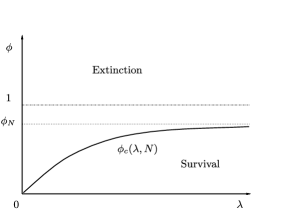
Figure 1: Phase diagram of Model $I$ for a fixed $N>1$ and finite initial configuration: by Theorem 3.2 there exists a critical curve $\phi_{c}(\lambda,N)$ which converges to $0$ as $\lambda$ goes to zero; it is always smaller than $1$. We conjecture that $\phi_{c}(\lambda,N)$ is monotone and as $\lambda$ goes to infinity converges to a value $\phi_{N}$ depending on the capacity $N$ of the model which is strictly smaller than $1$ for each $N<\infty$.

Figure 1 sketches the phase diagram in the $(\lambda,\phi)$ plane. The model admits a phase transition with respect to the death rate $\phi$ for each $N\geq 2$, while the same process without migrations dies out almost surely. The effect of a migration is to move an individual from a site in state $N$, where there is no possibility to give birth, to a site with less than $N$ individuals, where it may reproduce itself. Therefore even if there is no monotonicity with respect to $\lambda$ (cf. Remark 3.3), this suggests that an increase of $\lambda$ is good for survival. Contact interactions and migrations work in a similar way, but small differences are present. From a mathematical point of view an increase of the migration rate does not favor ergodicity.

4 Model II: The Allee effect

We translate the Allee effect into mathematical terms for a metapopulation model. As in Model I, we fix a capacity $N$ for all sites, but we assume the death rate larger than (or equal to) the birth rate when the density is small. Namely, fix a positive integer $N_{A}\leq N$ and positive real numbers $\phi$, $\lambda$ and $\phi_{A}\geq 1$; the transitions are, for all $x\in S$, $y\in S$, $x\sim y$, referring to the notation in (2)

$$\eta_{t}(x) \to \eta_{t}(x)+1\qquad\mbox{at rate }P^{1}_{\eta_{t}(x)}=\eta_{t}(x)\mathbh{1}_{\{\eta_{t}(x)\leq N-1\}},$$

$$\eta_{t}(x) \to \eta_{t}(x)-1$$

$$\eqntext{\displaystyle\mbox{at rate }P^{-1}_{\eta_{t}(x)}=\eta_{t}(x)\bigl{(}\phi_{A}\mathbh{1}_{\{\eta_{t}(x)\leq N_{A}\}}+\phi\mathbh{1}_{\{N_{A}<\eta_{t}(x)\}}\bigr{)},}$$ (21)

$$(\eta_{t}(x),\eta_{t}(y)) \to \bigl{(}\eta_{t}(x)-1,\eta_{t}(y)+1\bigr{)}$$

$$\eqntext{\displaystyle\mbox{at rate }\frac{1}{2d}\Gamma^{1}_{\eta_{t}(x),\eta_{t}(y)}=\frac{\lambda}{2d}\mathbh{1}_{\{\eta_{t}(x)=N,\eta_{t}(y)<N\}}.}$$ (22)

We assume $\phi_{A}\geq 1$ and $\phi_{A}\geq\phi$; in other words if $\eta_{t}(x)\leq N_{A}$, then the death rate $\phi_{A}\eta_{t}(x)$ is larger than (or equal to) the birth rate $\eta_{t}(x)$ because of the Allee effect. If $\eta_{t}(x)>N_{A}$, the most interesting situation is given by a death rate $\phi\eta_{t}(x)$ smaller than or equal to the birth rate $\eta_{t}(x)$, that is, $\phi\leq 1$. If either $\phi\geq 1$ and $\eta_{0}$ is finite or $\phi>1$ and $\eta_{0}\in\overline{\Omega}_{N}$ the species gets extinct as proved in Theorem 3.2. If $N_{A}=0$ (no Allee effect) or $N_{A}=N$ (death rate always larger than birth rate), there is only one death rate, and we are back to Model I.

Since only births, deaths and migrations of at most one particle are allowed, and the migration rate from $\eta_{t}(x)$ to $\eta_{t}(y)$ is nondecreasing in $\eta_{t}(x)$ and nonincreasing in $\eta_{t}(y)$, attractiveness conditions are satisfied. One proves in a similar way that Proposition 3.1 still holds for Model II either with respect to $\phi_{A}$ or $\phi$, namely:

Proposition 4.1

Let $(\xi_{t})_{t\geq 0}$ and $(\eta_{t})_{t\geq 0}$ be two Model II-type processes with respective parameters $(\phi_{1},\phi_{A,1},\lambda,N,N_{A})$ and $(\phi_{2},\phi_{A,2},\lambda,N,N_{A})$ such that $\phi_{1}\leq\phi_{2}$ and $\phi_{A,1}\leq\phi_{A,2}$. Then $(\xi_{t})_{t\geq 0}$ is stochastically larger than $(\eta_{t})_{t\geq 0}$, and $(\eta_{t})_{t\geq 0}$ is attractive.

Corresponding Corollary 3.2 holds in a similar way.

We prove that the Allee effect changes the behavior of the system: for any possible capacity $N$ and migration rates there exists an Allee effect large enough for the species to become extinct.

Theorem 4.1

Assume $\phi_{A}\geq 1$, and let $\phi_{c}(\lambda,N)$ be the critical parameter introduced in Theorem 3.2. Then for all $\lambda>0$, $0<N<\infty$, $0<N_{A}\leq N$: [(ii)]

if $\phi<\phi_{c}(\lambda,N)$, there exists a value $\phi^{A}_{c}(\phi,\lambda,N,N_{A})$ such that if $\phi_{A}>\phi^{A}_{c}(\phi,\lambda,N,N_{A})$, the species becomes extinct for any initial configuration $\eta_{0}\in\Omega_{N}$, and if $\phi_{A}<\phi^{A}_{c}(\phi,\lambda,N,N_{A})$ the species has a positive probability of survival;

if $\phi_{c}(\lambda,N)<\phi$ $(\leq\phi_{A})$, the species becomes extinct for any initial configuration $\eta_{0}\in\Omega_{N}$.

This corresponds to the biological idea that random fluctuations, which are present on each local population, plus the Allee effect doom even a very large population.

The phase diagram of Model II depends on $\phi_{A}$. Proposition 4.1 is not enough to construct a detailed phase diagram, but it gives some information in this direction. Since for any $\phi$ and $\lambda$ there exists $\phi_{A}$ large enough for the species to become extinct, one can choose $\phi_{A}$ large enough to reduce the survival region in the $(\lambda,\phi)$ plane of Figure 1 for such fixed $\phi_{A}$.

In order to model the Allee effect, we require $\phi_{A}\geq 1$ and $\phi\leq 1$. Note that from a biological point of view we just need $\phi_{A}>\phi$, but if either $\phi_{A}>\phi>1$ or $1>\phi_{A}>\phi$, by monotonicity arguments we can work as in Model I.

From a mathematical point of view, it would be interesting to investigate a model where $\phi$ and $\phi_{A}$ play symmetric roles, that is, $\phi_{A}\leq 1$ and $\phi\geq 1$. For fixed $N$, $N_{A}$ and $\lambda$ we prove that there is no $\phi_{A}$ such that there is survival for all $\phi$ and no $\phi$, such that there is extinction for all $\phi_{A}$.

Theorem 4.2

For all $1<N_{A}<N$, $\lambda>0$: [(ii)]

for each $\phi>1$ there exists a value $\phi^{A}_{c}(\lambda,N_{A},N,\phi)$ such that, if $\phi_{A}<\phi^{A}_{c}(\lambda,N_{A},N,\phi)$, the process survives for any initial configuration $\eta_{0}$ such that $|\eta_{0}|\geq 1$ with positive probability;

for each $\phi_{A}<1$ there exists a value $\phi_{c}(\lambda,N_{A},N,\phi_{A})$ such that, if $\phi>\phi_{c}(\lambda,N_{A},N,\phi_{A})$, the process dies out for any initial configuration $\eta_{0}\in\Omega_{N}$.

5 Model III: Mass migration as Allee effect solution

We have already observed in Model I that a migration of a single individual is good in absence of the Allee effect. The model without migrations dies out, but if we add a possible migration of one individual there is a positive probability of survival. In Model II, anyhow, a single individual migration may not be enough: even in the supercritical region of $\phi$ in Model I there exists an Allee effect strong enough for the species to become extinct.

Which strategy may a species adopt to reduce the Allee effect?

We show that, at least in theory, migrations of large flocks of individuals improve the probability of survival for any Allee effect. A migration of many individuals in a new environment improves the probability of a successful colonization avoiding a small density in that new environment which is influenced by the Allee effect.

We introduce positive parameters $\phi_{A}$, $\phi$, $N_{A}$, $N$ such that $0\leq N_{A}\leq N$, $\phi_{A}>1$, $\phi>0$ and we take birth and death transitions as in Model II, but more general migration rates: given $M\in\mathbb{N}$, $0<M\leq N$, $y\sim x$ the transitions are

$$\eta_{t}(x) \to \eta_{t}(x)+1\qquad\mbox{at rate }P^{1}_{\eta_{t}(x)}=\eta_{t}(x)\mathbh{1}_{\{\eta_{t}(x)\leq N-1\}},$$

$$\eta_{t}(x) \to \eta_{t}(x)-1$$

$$\eqntext{\displaystyle\mbox{at rate }P^{-1}_{\eta_{t}(x)}=\eta_{t}(x)\bigl{(}\phi_{A}\mathbh{1}_{\{\eta_{t}(x)\leq N_{A}\}}+\phi\mathbh{1}_{\{N_{A}<\eta_{t}(x)\}}\bigr{)},}$$ (24)

$$(\eta_{t}(x),\eta_{t}(y)) \to \bigl{(}\eta_{t}(x)-k,\eta_{t}(y)+k\bigr{)}$$

$$\eqntext{\displaystyle\mbox{at rate }\frac{1}{2d}\Gamma^{k}_{\eta_{t}(x),\eta_{t}(y)}=\frac{\lambda}{2d}\mathbh{1}_{\{\eta_{t}(x)-k\geq N-M,\eta_{t}(y)+k\leq N\}}}$$ (25)

for $1\leq k\leq M$. In other words if $k\in\{1,2,\ldots,M\}$ individuals try to migrate from $x$ to $y$, but if $\eta_{t}(y)+k>N$, the migration does not happen. Notice that if $\eta_{t}(x)<N-M$ the migration rate is null: individuals try to migrate only when there are more than $N-M$ individuals on a site. From a biological point of view, this means that when there are few individuals, resources are enough for all and there are no reasons to migrate. When $\eta_{t}(x)\geq N-M$ there is a positive probability of migration and the number of individuals that may migrate is increasing with the population size. If $\eta_{t}(x)=N-M+1$ we allow a migration of at most $1$ individual from $x$ to a nearest neighbor site; when $\eta_{t}(x)=N-M+2$ we allow a migration of either $1$ or $2$ individuals with rate $\lambda$ and so on. If $\eta_{t}(x)=N=(N-M)+M$ we allow a migration of $1,2,\ldots$ to the largest flock of $M$ individuals, where each migration occurs with rate $\lambda$.

First of all we notice monotonicity properties.

Proposition 5.1

Let $(\xi_{t})_{t\geq 0}$ and $(\eta_{t})_{t\geq 0}$ be two Model III-type processes with respective parameters $(\phi_{1},\phi_{A,1},\lambda,N,N_{A})$ and $(\phi_{2},\phi_{A,2},\lambda,N,N_{A})$ such that $\phi_{1}\leq\phi_{2}$ and $\phi_{A,1}\leq\phi_{A,2}$. Then $(\xi_{t})_{t\geq 0}$ is stochastically larger than $(\eta_{t})_{t\geq 0}$, and $(\eta_{t})_{t\geq 0}$ is attractive.

Corresponding Corollary 3.2 holds in a similar way.

In Model II we showed that a strong Allee effect dooms even a very large population with a large migration rate. The strategy that the species may adopt to reduce the Allee effect is to increase the number of individuals which migrate: we prove that we can take a population size $N$ and a maximal migration flock size $M$ large enough for the species to survive for any Allee effect.

Theorem 5.1

Let $d\geq 2$. For all $\lambda>0$, $N_{A}\geq 0$: [(ii)]

if $\phi<1$ there exists $N_{c}(\phi,\lambda,N_{A})$ such that for each $N>N_{c}(\phi,\lambda,N_{A})$, there exists $M(N_{A})$ so that the process starting from $\eta_{0}$ with $|\eta_{0}|\geq 1$ has a positive probability of survival for each $\phi_{A}<\infty$. Moreover if $\eta_{0}\in\overline{\Omega}_{N}$ the process converges to a nontrivial invariant measure for each $\phi_{A}<\infty$;

if $\phi\geq 1$, the process becomes extinct for all $N$, $\lambda$, $\phi_{A}>1$, $M$ and for any finite initial configuration. If $\eta_{0}\in\Omega_{N}$ is not finite the process becomes extinct if $\phi>1$.

Remark 5.2.

The proof of (i) (see Section 7) states that in order to have survival we can take $M(N_{A})=N_{A}+1$. If $N_{A}=0$, this gives $M(N_{A})=N_{A}+1=1$; only a migration of one individual is possible and the process reduces to a Model I-type process: therefore Theorem 3.1 is a particular case of Theorem 5.1.

Notice that $N_{c}(\phi,\lambda,N_{A})$ does not depend on $\phi_{A}$. This means that even if the Allee effect is the strongest one, if the species lives and migrates in flocks large enough, survival is possible.

Since there are many parameters the phase diagram is not easy to construct; nevertheless Proposition 5.1 suggests that one can choose $N$ and $M$ large enough to extend the survival region in the $(\lambda,\phi)$-plane for fixed $\phi_{A}$, $N$ and $M$.

6 Model IV: Ecological equilibrium

Real natural environments do not have any a priori bound on the population size, but there is a kind of self-regulating mechanism that does not allow an “explosion” of the number of individuals per site. Ecological equilibrium has been introduced in cfBertacchi for restrained branching random walks (on a connected, nonoriented graph $X$ with bounded geometry) with transition rates

$$\eta(x) \to \eta(x)+1\qquad\mbox{at rate }\sum_{y}\eta(y)p(y,x)c(\eta(x)),$$

$$\eta(x) \to \eta(x)-1\qquad\mbox{at rate }\eta(x),$$

where $c\dvtx\mathbb{N}\to\mathbb{R}^{+}$ is a nonincreasing function and $P=(p(x,y))_{x,y\in X}$ is a stochastic matrix such that $p(x,y)>0$ only if $x\sim y$. The idea is that some restrictions on branching random walks birth rates, given by the nonincreasing function $c(\cdot)$ of the number of individuals, provide survival within nonexploding populations. In particular, one interesting consequence of cfBertacchi , Proposition 1.1, is that one can find a function $c$ such that the process survives but $\limsup_{t\to\infty}\mathbb{E}^{\eta_{0}}(\eta_{t}(x))<\infty$ uniformly for any bounded $\eta_{0}\in\Omega$ and $x\in X$.

We show that a similar mechanism leads to a similar conclusion on different systems. Instead of taking births on neighboring sites as in cfBertacchi , we consider a nonincreasing birth rate in the same local population, but we add migrations when the number of individuals is larger than a fixed value $N$. This means that the restriction on birth rate does not change the migration rate: this is not the case for the restrained branching random walk, where births in a new site (which play the same role as migrations in Model IV) depend on the local population density.

We suppose that in our environment there is no maximal population size as in previous models, and the birth rate is always positive. We also assume that, when the population size is larger than $N$, the death rate increases faster than the birth rate, hence the growth rate is negative.

In order to simplify notation and proofs, we work on a modification of Model I. Namely, given positive real values $\phi$, $\widetilde{\phi}$, we take the following transitions, for each $x\in S$, $y\in S$, $x\sim y$:

$$\eta_{t}(x) \to \eta_{t}(x)+1\qquad\mbox{at rate }P^{1}_{\eta_{t}(x)}=\eta_{t}(x),$$

$$\eta_{t}(x) \to \eta_{t}(x)-1$$

$$\eqntext{\displaystyle\mbox{at rate }P^{-1}_{\eta_{t}(x)}=\eta_{t}(x)\bigl{(}\phi\mathbh{1}_{\{\eta_{t}(x)\leq N\}}+{\widetilde{\phi}}\mathbh{1}_{\{N<\eta_{t}(x)\}}\bigr{)},}$$ (27)

$$(\eta_{t}(x),\eta_{t}(y)) \to \bigl{(}\eta_{t}(x)-1,\eta_{t}(y)+1\bigr{)}$$

$$\eqntext{\displaystyle\mbox{at rate }\frac{1}{2d}\Gamma^{1}_{\eta_{t}(x),\eta_{t}(y)}=\frac{\lambda}{2d}\mathbh{1}_{\{\eta_{t}(x)\geq N,\eta_{t}(y)<N\}}.}$$ (28)

This means that when the population size $\eta_{t}(x)$ is larger than $N$, and the death rate $\widetilde{\phi}\eta_{t}(x)$ is larger than the birth rate $\eta_{t}(x)$. A migration is allowed from a site with more than $N$ individuals to a site with less than $N$ individuals. Since we are working without any a priori bound, we refer to construction techniques in noncompact cases, and we restrict the state space to $\widetilde{\Omega}\subseteq\Omega$ (see cfChenbook , Chapter 13), where

$$\widetilde{\Omega}:=\biggl{\{}\eta\in\Omega\dvtx\sum_{x\in\mathbb{Z}^{d}}\eta(x)\alpha(x)<\infty\biggr{\}},$$

and $(\alpha(x))_{x\in\mathbb{Z}^{d}}$ is a positive sequence such that $\sum_{x\in\mathbb{Z}^{d}}\alpha(x)<\infty$. Sufficient conditions for existence and uniqueness of the process given in cfChenbook , Chapter 13, are satisfied:

Lemma 6.1

There exists a unique Markov process with state space $\widetilde{\Omega}$, generator (2) and rates (6).

Since births, deaths and migrations involve only one particle and the migration rate is nondecreasing in $\eta_{t}(x)$ and nonincreasing in $\eta_{t}(y)$ the process is attractive as in Model I, and a monotonicity property (see Proposition 3.2) holds in $\phi$ and in $\widetilde{\phi}$ for each initial configuration $\eta_{0}\in\widetilde{\Omega}$. We prove that in some cases the process survives but does not explode; that is, it does not die out, and the expected value on each site is finite.

Theorem 6.1

Let $\eta_{0}\in\Omega_{n}$ for some $n\in\mathbb{N}$ (so that $\eta_{0}\in\widetilde{\Omega}$). For all $\lambda>0$, ${\widetilde{\phi}}>1$: [(ii)]

for each $1<N<\infty$ there exists a critical value $\phi_{c}(\lambda,N,{\widetilde{\phi}})>0$ such that if $\phi<\phi_{c}(\lambda,N,{\widetilde{\phi}})$, the process has a positive probability of survival, and if $\phi>\phi_{c}(\lambda,N,{\widetilde{\phi}})$ the process dies out;

for each $\phi<1$ there exists a value $N_{c}(\lambda,\phi,{\widetilde{\phi}})>0$, such that if $N>N_{c}(\lambda,\phi,{\widetilde{\phi}})$, the process has a positive probability of survival.

If the process survives, there exists $C_{n}<\infty$ so that $\lim_{t\to\infty}\mathbb{E}(\eta_{t}(x))\leq C_{n}$ for each $x\in\mathbb{Z}^{d}$.

Note that the constant $C_{n}$ depends on the initial configuration. Since the migration rate does not depend on the local population density, we are not able to find such a constant $C$ independent of the initial configuration, which was the case for the model treated in cfBertacchi .

Remark 6.2.

In a similar way one can consider a Model III-type process without any a priori bound by adding a death rate $\widetilde{\phi}\eta_{t}(x)$ when the number of individuals in a local population is larger than $N$. By comparison arguments, even if a strong Allee effect is present, a mass migration of large flocks of individuals leads to the survival of the species, but the local populations do not explode.

7 Proofs

We first recall a classical result involving random walks on a finite interval. Let $r_{1},r_{2}\in\mathbb{N}$ and $(X_{t})_{t\geq 0}$ be a discrete time random walk on $\{r_{1},r_{1}+1,\ldots,r_{2}=r_{1}+n\}$ such that

$$i \to i+1\mbox{ with probability }p,\qquad i\in\{r_{1},\ldots,r_{2}-1\},$$

$$i \to i-1\mbox{ with probability }q,\qquad i\in\{r_{1}+1,\ldots,r_{2}\}.$$

We interpret this random walk as a game which ends when $X_{t}$ reaches either $r_{1}$ or $r_{2}$, that we call respectively the ruin of the first and the second players.

Lemma 7.1 ((Ruin Problem Formula, bookschinazi , (4.4), Section I.4))

Let $P_{r_{2}}(j)$ [resp., $P_{r_{1}}(j)$] be the probability that the random walk starting at $j\in\{r_{1}+1,\ldots,r_{2}-1\}$ reaches state $r_{2}$ before state $r_{1}$ (resp., state $r_{1}$ before $r_{2}$). Then

$$1-P_{r_{1}}(j)=P_{r_{2}}(j)=\frac{1-(q/p)^{j-r_{1}}}{1-(q/p)^{n}}.$$

7.1 Model I

7.1.1 Proof of Proposition 3.1

We prove that if $\eta_{0}\leq\xi_{0}$, then $\eta_{t}\leq\xi_{t}$ for each $t>0$ a.s. This is an application of Theorem 2.1; since there is a change of at most one particle per time, we check conditions in Remark 2.4. The transition rates are given by (3), with $\phi=\phi_{2}$ for the process $(\eta_{t})_{t\geq 0}$ and $\phi=\phi_{1}$ for $(\xi_{t})_{t\geq 0}$. Conditions (13) and (14) are the following: given $\eta\leq\xi$, if $\eta(y)=\xi(y)$ and $\eta(x)\leq\xi(x)$

$$\eta(y)\mathbh{1}_{\{\eta(y)\leq N-1\}}+\lambda\mathbh{1}_{\{\eta(x)=N,\eta(y)<N\}} \leq \xi(y)\mathbh{1}_{\{\xi(y)\leq N-1\}}+\lambda\mathbh{1}_{\{\xi(x)=N,\xi(y)<N\}},$$

$$\eta(y)\mathbh{1}_{\{\eta(y)\leq N-1\}} \leq \xi(y)\mathbh{1}_{\{\xi(y)\leq N-1\}}.$$

Since $\eta\leq\xi$ and $\eta(x)=N$ imply $\xi(x)=N$, and since $\mathbh{1}_{\{\eta(x)=N,\eta(y)<N\}}\leq\mathbh{1}_{\{\xi(x)=N,\xi(y)<N\}}$ if $\eta(y)=\xi(y)$, the conditions are satisfied.

Conditions (15) and (16) are the following: if $\eta(x)=\xi(x)$ and $\eta(y)\leq\xi(y)$,

$$\phi_{2}\eta(x)\mathbh{1}_{\{\eta(x)\leq N-1\}}+\lambda\mathbh{1}_{\{\eta(x)=N,\eta(y)<N\}}$$

$$\qquad\geq\phi_{1}\xi(x)\mathbh{1}_{\{\xi(x)\leq N-1\}}+\lambda\mathbh{1}_{\{\xi(x)=N,\xi(y)<N\}},$$

$$\phi_{2}\eta(x)\mathbh{1}_{\{\eta(x)\leq N-1\}}\geq\phi_{1}\xi(x)\mathbh{1}_{\{\xi(x)\leq N-1\}},$$

which hold since $\phi_{2}\geq\phi_{1}$ and $\mathbh{1}_{\{\eta(x)=N,\eta(y)<N\}}\geq\mathbh{1}_{\{\xi(x)=N,\xi(y)<N\}}$, because $\eta(x)=\xi(x)$.

7.1.2 Proof of Theorem 3.2

We prove it in three steps. In Step (i) we find $\phi^{1}_{c}(\lambda,N)$ small enough to have survival; in Step (ii) we prove that the process dies out for all $\lambda,N$ by taking $\phi\geq 1$ if it starts from a finite initial configuration and by taking $\phi>1$ it it starts from $\eta_{0}\in\overline{\Omega}_{N}$, and in Step (iii) we get the existence of a critical parameter by monotonicity.

(i) We follow the idea in cfschivirus by using the comparison technique with oriented percolation (introduced in cfBramsonDurrett ) explained in cfdurrettten . Here and in the subsequent proofs we think of the process as being generated by the graphical representation; see cfdurrettten for such a construction. Suppose $d=2$. The proof in higher dimension is similar, but the notation is more complicated. Denote by

$$\qquad\cases{e_{1}=(1,0),&\quad$\mathcal{N}=\{(m,n)\in\mathbb{Z}^{2}\dvtx m+n\mbox{ is even}\},$\vspace*{1pt}\cr B=(-4L,4L)^{2}\times[0,T],&\quad$B_{m,n}=(2mLe_{1},nT)+B,$\vspace*{1pt}\cr I=[-L,L]^{2},&\quad$I_{m}=2mLe_{1}+I,$}$$ (29)

where $L$ and $T$ are integers to be chosen later. In other words $B_{m,n}$ is the cube that we get by applying a translation of $(2mLe_{1},nT)$ to $B$ and $I_{m}$ the square we get by applying a translation of $2mLe_{1}$ to $I$. Roughly speaking, the idea consists of constructing boxes large enough so that with large probability the species survives inside a box, and then to compare this evolution with an oriented percolation model.

Let $(\eta_{t})_{t\geq 0}$ be the process defined by generator (2) with rates (3). We consider a modification $\eta^{m,n}_{t}$ of $\eta_{t}$: the process $(\eta^{m,n}_{t})_{t\geq 0}$ is constructed through the graphical representation of $\eta_{t}$ in $B_{m,n}$, but $\eta_{t}(x)=0$ for all $x\notin B_{m,n}$ and $t\geq 0$. Let $m_{x,y}$ with $y\sim x$ be the Poisson process with rate $\lambda/(2d)$ associated to a migration from $x$ to $y$. A migration from $x$ belongs to the graphical construction in $B_{m,n}$ if $x\in B_{m,n}$: therefore an immigration to $B_{m,n}$ from a site $y\notin B_{m,n}$ cannot happen for $\eta^{m,n}_{t}$, but we still consider the arrows of emigrations from $B_{m,n}$. Their effect is the death of one individual on the boundary of $B_{m,n}$. If $\eta_{0}(x)=\eta_{0}^{m,n}(x)=\mathbh{1}_{\{y\}}(x)$ for some $y\in B_{m,n}$, $\eta_{t}\geq\eta^{m,n}_{t}$ by Remark 2.4 since if $x\notin B_{m,n}$, then $\eta^{m,n}_{t}(x)=0$; otherwise conditions in Remark 2.4 are satisfied for each pair of sites $(x,y)$; see also Remark 2.5.

We say that $(m,n)$ is wet if $\eta^{m,n}_{t}$ starting at time $nT$ with at least one individual in $I_{m}$ is such that there is at least one individual in $I_{m-1}$ and one individual in $I_{m+1}$ at time $(n+1)T$. Otherwise the site is dry. The event $G_{m,n}:=\{(m,n)\mbox{ is wet}\}$ is measurable with respect to the graphical construction in $B_{m,n}$: we prove that we can choose $L$ and $T$ such that the probability of a site $(m,n)$ to be wet can be made arbitrarily close to $1$ if $\phi$ is small enough. By translation invariance it is enough to show it for $(0,0)$. We call $\eta^{0,0}_{t}:=\xi_{t}$, we fix $L>0$ and we prove that for each $\varepsilon>0$ there exists $T$ and $\phi$ such that

$$\mathbb{P}\bigl{(}(0,0)\mbox{ is wet}\bigr{)}\geq 1-\varepsilon,$$ (30)

that is, that if there exists one individual in a site $(i,j)\in I_{0}=:I$, there is at least one individual both in $I_{1}$ and $I_{-1}$ with large probability.

In order to prove it for $\phi$ small enough, we begin by showing that it holds for a process with $\phi=0$ inside $B$: let $\widetilde{\mathbb{P}}(\xi_{t}\in\cdot)$ denote the law of such a process. This means that each individual in box $B$ survives forever.

We choose a preferential path $(i,j),(i+1,j),\ldots,(L,j),(L+1,j)$: we prove that there exists $T$ large enough so that the abscissas of the rightmost and leftmost particles are respectively larger than $L$ and smaller than $-L$ with probability larger than $1-\varepsilon$, since this is one possibility for the site $(0,0)$ to be wet.

A similar idea works for the leftmost particle. We conclude that if $\phi=0$ for all $\varepsilon>0$, $\lambda>0$, $1<N<\infty$ there exists $T=L\overline{T}$ such that

$$\widetilde{\mathbb{P}}\bigl{(}(0,0)\mbox{ is wet}\bigr{)}>1-\varepsilon/2.$$ (31)

Now we prove (30) for $\phi$ small enough. Let $A_{L}=A_{L}(\phi,N)$ be the time of the first death on the finite box $(-4L,4L)^{2}$. If $A_{L}>T:=L\overline{T}$, for each $\varepsilon>0$ we can take $\phi>0$ small enough for

$$\mathbb{P}\bigl{(}(0,0)\mbox{ is wet}\bigr{)} \geq \mathbb{P}\bigl{(}(0,0)\mbox{ is wet}|A_{L}>T\bigr{)}\mathbb{P}(A_{L}>T)$$

$$\geq \widetilde{\mathbb{P}}\bigl{(}(0,0)\mbox{ is wet}\bigr{)}e^{-\phi N(8L)^{2}T}\geq 1-\varepsilon.$$

Hence for all $\varepsilon>0$, $L>0$, $\lambda>0$, $1<N<\infty$ there exists $T$ and $\phi^{1}_{c}(\lambda,N)>0$ such that if $\phi\leq\phi^{1}_{c}(\lambda,N)$, then (30) holds.

By comparing the process with an oriented percolation process, the existence of an infinite path of wet sites corresponds to the existence of individuals at all times, and for $\varepsilon$ small enough percolation occurs; see cfdurrettten . By monotonicity (Proposition 3.1), the process survives for any $\phi\leq\phi^{1}_{c}(\lambda,N)$.

(ii) Let $\xi_{t}$ be a continuous-time Galton–Watson process without spatial structure starting from $|\eta_{0}|\leq\xi_{0}$ individuals. We couple the total number of particles of the two processes. Each individual in both processes breeds at rate $1$ (except for $\eta_{t}$ when the full carrying capacity of the site is reached) and dies at rate $\phi$. Since we are interested in the total number of particles, migrations do not count in this coupling. Therefore $|\eta_{t}|\leq\xi_{t}$ for all $t\geq 0$. If $\xi_{0}$ is finite and $\phi\geq 1$, then the Galton–Watson process becomes extinct; this implies that $\eta_{t}$ dies out for any $\phi\geq 1$.

Assume now that $\eta_{0}\in\overline{\Omega}_{N}$; we prove that the process becomes extinct when $\phi>1$. By translation invariance, for each $t>0$,

$$\frac{d}{dt}\mathbb{E}(\eta_{t}(x)) = \mathbb{E}(\mathcal{L}\eta_{t}(x))$$

$$= \mathbb{E}\biggl{(}\eta_{t}(x)\mathbh{1}_{\{\eta_{t}(x)\leq N-1\}}-\phi\eta_{t}(x)+\sum_{y\sim x}\mathbh{1}_{\{\eta_{t}(y)=N,\eta_{t}(x)<N\}}\lambda/(2d)$$

$$\hskip 113.0pt\qquad{}-\sum_{y\sim x}\mathbh{1}_{\{\eta_{t}(x)=N,\eta_{t}(y)<N\}}\lambda/(2d)\biggr{)}$$

$$= \mathbb{E}\bigl{(}\eta_{t}(x)\mathbh{1}_{\{\eta_{t}(x)\leq N-1\}}-\phi\eta_{t}(x)\bigr{)}\leq(1-\phi)\mathbb{E}(\eta_{t}(x)),$$

and by Gronwall’s lemma the process converges to $0$ uniformly with respect to $x$. By Corollary 3.2 the process dies out for each $\phi>1$.

(iii) The claim follows by Steps (i), (ii) and Corollary 3.2. Starting from $\eta_{0}\in\overline{\Omega}_{N}$, the existence of the upper invariant measure follows from attractiveness, and it is nontrivial by Step (i).

7.2 Model II

7.2.1 Proof of Theorem 4.1

(ii) Since $\phi_{A}\geq\phi$, Model $I$ is stochastically larger than Model $\mathit{II}$. If $\phi>\phi_{c}(\lambda,N)$, both of them die out by Theorem 3.2.

(i) Assume $\phi<\phi_{c}(\lambda,N)$ ($\leq 1$ by Theorem 3.2). We follow the idea in Berg , Theorem 4.4, and we compare the system with a subcritical percolation process. We prove (i) when $d=2$ in order to simplify the notation (the same proof works for all $d\geq 1$). Let $(\eta_{t})_{t\geq 0}$ be a process with generator $(\ref{generator})$, rates $(\ref{rates2})$ and $\eta_{0}\in\overline{\Omega}_{N}$. We define

$$\qquad\cases{\mathcal{A}=[-2L,2L]^{2}\times[0,2T];\qquad\mathcal{B}=[-L,L]^{2}\times[T,2T],\vspace*{2pt}\cr\mathcal{C}_{b}=\{(x,y,t)\in\mathcal{A}\dvtx t=0\},\vspace*{2pt}\cr\mathcal{C}_{s}=\{(x,y,t)\in\mathcal{A}\dvtx|x|=2L\mbox{ or }|y|=2L\},\vspace*{2pt}\cr\mathcal{C}=\mathcal{C}_{b}\cup\mathcal{C}_{s}=\{(x,y,t)\in\mathcal{A}\dvtx|x|=2L\mbox{ or }|y|=2L\mbox{ or }t=0\},}$$ (32)

where $T$ is a time to be fixed later.

In other words $\mathcal{C}$ is part of the boundary of the space–time region $\mathcal{A}$, which contains the smaller region $\mathcal{B}$. We construct a percolation process on $\mathcal{N}=\mathbb{Z}^{2}\times\mathbb{Z}_{+}$ starting from $(\eta_{t})_{t\geq 0}$. We consider for each $(m,n,k)\in\mathcal{N}$ a modification $\eta^{m,n,k}_{t}$ of $\eta_{t}$: the process $(\eta^{m,n,k}_{t})_{t\geq 0}$ is constructed through the graphical representation of $\eta_{t}$ in $\mathcal{A}+(mL,nL,kT)$, but $\eta^{m,n,k}_{t}(x)=N$ for all $x\in(mL,nL)+(-2L,2L)^{2}$, $t\leq kT$ and $x\notin(mL,nL)+(-2L,2L)^{2}$ for all $t\geq 0$. Therefore an emigration from $\mathcal{A}+(mL,nL,kT)$ cannot happen and an immigration from a site $y$ on the boundary of $(mL,nL)+[-2L,2L]^{2}$ after $kT$ is always possible with rate $\lambda$. By Remarks 2.4 and 2.5, $\eta_{t}\leq\eta_{t}^{m,n,k}$ for all $m$, $n$, $k$ and $t\geq 0$, since if $x\notin(mL,nL)+(-2L,2L)^{2}$, then $\eta^{m,n}_{t}(x)=N$, otherwise conditions in Remark 2.4 are satisfied for each pair of sites $(x,y)$.

We say that a site $(m,n,k)\in\mathcal{N}$ is wet if there are no individuals for the process $\eta^{m,n,k}_{t}$ in $\mathcal{B}+(mL,nL,kT)$. A site is dry if it is not wet.

We show, through a series of lemmas, that the probability of a site to be wet is as large as we want by taking $\phi_{A}$ large. By translation invariance we prove it for $(0,0,0)$, and we denote $\eta^{0,0,0}_{t}:=\xi_{t}$. Let $0<\phi_{A}<\infty$. First of all we prove that there exists a time $S$ at which with large probability there is at most $1$ individual per site on $(-2L,2L)^{2}$ (Lemma 7.3). After $S$, there exists a time $T$ such that there are no individuals in $(-2L,2L)^{2}$ with large probability (Lemma 7.4). Therefore with large probability the only possibility of having one individual in $\mathcal{B}$ is that an emigration from the boundary after time $T$ reaches $[-L,L]^{2}$ before $2T$: the last step consists in proving that such an event has small probability.

We first introduce an auxiliary process whose transitions are not translation invariant:

Lemma 7.2

Let $(\overline{\xi}_{t})_{t\geq 0}$ be a process with only birth and death rates: if $x\in(-2L,2L)^{2}$

$$\overline{P}^{1}_{l}(x)=\mathbh{1}_{\{l\leq N-1\}}(l+\lambda);\qquad\overline{P}^{-1}_{l}(x)=l\bigl{(}\phi_{A}\mathbh{1}_{\{l\leq N_{A}\}}+\phi\mathbh{1}_{\{N_{A}<l\}}\bigr{)}$$ (33)

and $\overline{\xi}_{t}(x)=N$ for all $x\notin(-2L,2L)^{2}$, $t\geq 0$. Then $(\overline{\xi}_{t})_{t\geq 0}$ is stochastically larger than $(\xi_{t})_{t\geq 0}$.

Both $\xi_{t}$ and $\overline{\xi}_{t}$ are equal to $N$ for each $t\geq 0$ outside $(-2L,2L)^{2}$. By Remark 2.5, we check the conditions in Remark 2.4 for each pair of sites $(x,y)$ with either $x$ or $y$ in $(-2L,2L)^{2}$. If $x\in(-2L,2L)^{2}$, $(\overline{\xi}_{t}(x))_{t\geq 0}$ is a birth and death process whose birth rate is the original one plus the largest immigration rate on $\xi_{t}(x)$, and whose death rate is the original one plus the smallest emigration rate on $\xi_{t}(x)$, which is null. For each $\eta\in\Omega$,

$$P^{1}_{\eta(y)}+\Gamma^{1}_{\eta(x),\eta(y)} \leq \mathbh{1}_{\{\eta(y)\leq N-1\}}\bigl{(}\eta(y)+\lambda\bigr{)}=\overline{P}^{1}_{\eta(y)},$$

$$P^{-1}_{\eta(x)}+\Gamma^{1}_{\eta(x),\eta(y)} \geq \mathbh{1}_{\{\eta(x)\leq N_{A}\}}\phi_{A}\eta(x)+\mathbh{1}_{\{N_{A}<\eta(x)\}}\phi\eta(x)=\overline{P}^{-1}_{\eta(x)};$$

then all conditions are satisfied.

Lemma 7.3

For all $\varepsilon>0$, $L$ there exists $S>0$ and $\phi_{A}$ such that

$$\mathbb{P}(G_{L}(S))>1-\varepsilon/6,$$ (34)

where $G_{L}(S)=\{\xi_{S}(x)\leq 1\mbox{ for each }x\in(-2L,2L)^{2}\}$.

We prove (34) for $(\overline{\xi}_{t})_{t\geq 0}$ with law $\overline{\mathbb{P}}(\overline{\xi}_{t}\in\cdot)$. By monotonicity (Lemma 7.2) it will be true for $(\xi_{t})_{t\geq 0}$. For all $\varepsilon>0$ and $L$ we take $S$ large enough so that the number of visits $H^{S}_{x}$ to $0$ of $\overline{\xi}_{t}(x)$ before $S$ satisfies

$$\overline{\mathbb{P}}(H^{S}_{x}=0)\leq\frac{\varepsilon}{18(4L)^{2}}.$$ (35)

If there is at least one visit, we consider

$$\sum_{k=1}^{K}\overline{\mathbb{P}}\bigl{(}\overline{\xi}_{S}(x)>1|H^{S}_{x}=k\bigr{)}\overline{\mathbb{P}}(H^{S}_{x}=k)$$

(36)

$$\qquad{}+\sum_{k=K+1}^{\infty}\overline{\mathbb{P}}\bigl{(}\overline{\xi}_{S}(x)>1|H^{S}_{x}=k\bigr{)}\overline{\mathbb{P}}(H^{S}_{x}=k).$$

By taking $K$ large enough the second sum (in which there are more than $K$ hits to $0$) is as small as we want. There are at least two individuals in a site after the $i$th visit to $0$ only if the exponential clock $B_{i}\sim\operatorname{Exp}(1+\lambda)$ [birth rate if $\overline{\xi}_{t}(x)=1$] rings before the one of $D_{i}\sim\operatorname{Exp}(\phi_{A})$ [death rate if $\overline{\xi}_{t}(x)=1$]. Therefore for all $\varepsilon>0$, $L$ and $K$ we can take $\phi_{A}$ large enough for the first sum in (7.2.1) to be smaller than

$$\qquad\sum_{k=1}^{K}\overline{\mathbb{P}}(\exists i\in\{1,2,\ldots,k\}\dvtx B_{i}<D_{i})\leq K^{2}\frac{1+\lambda}{1+\lambda+\phi_{A}}\leq\frac{\varepsilon}{18(4L)^{2}}.$$ (37)

By (35) and (37) for all $\varepsilon>0$, $L$ there exists $S$ and $\phi_{A}$ large enough for

$$\mathbb{P}((G_{L}(S))^{c})\leq(4L)^{2}\sup_{x\in(-2L,2L)^{2}}\overline{\mathbb{P}}\bigl{(}\overline{\xi}_{S}(x)>1\bigr{)}\leq\varepsilon/6,$$ (38)

and the claim follows.

Lemma 7.4

For all $L$, $\varepsilon>0$ there exists $\overline{S}$ and $\phi_{A}$ such that

$$\mathbb{P}\bigl{(}\overline{G}_{L}(S+\overline{S})\bigr{)}\geq 1-\varepsilon/3,$$

where $\overline{G}_{L}(S+\overline{S})=\{\xi_{S+\overline{S}}(x)=0\mbox{ for each }x\in(-2L,2L)^{2}\}$, and $S$ is given by Lemma 7.3.

If $G_{L}(S)$ holds, we take $\overline{S}$ small so that there are neither births nor immigrations from the boundary $\mathcal{C}_{s}$ between $S$ and $\overline{S}$ and $\phi_{A}$ large so that all individuals in $(-2L,2L)^{2}$ die before $\overline{S}$ with large probability. Namely, given $D\sim\operatorname{Exp}(\phi_{A})$ and $B\sim\operatorname{Exp}((1+\lambda)(4L-1)^{2})$, for all $\varepsilon>0$, $L$ there exists $\overline{S}$ small and $\phi_{A}(\overline{S})$ large enough for

$$\mathbb{P}\bigl{(}\overline{G}_{L}(S+\overline{S})|G_{L}(S)\bigr{)} \geq \mathbb{P}(D<\overline{S})^{(4L-1)^{2}}\mathbb{P}(\overline{S}<B)$$

$$\geq \bigl{(}1-\exp(-\phi_{A}\overline{S})\bigr{)}^{(4L-1)^{2}}\exp\bigl{(}-(1+\lambda)(4L-1)^{2}\overline{S}\bigr{)}$$

$$\geq 1-\varepsilon/6.$$

If $T=S+\overline{S}$, given by the two previous lemmas,

$$\mathbb{P}((\overline{G}_{L}(T))^{c})\leq\varepsilon/6+\varepsilon/6=\varepsilon/3,$$ (39)

and the claim follows.

Therefore $\xi_{T}(x)=0$ for each $x\in(-2L,2L)^{2}$ with large probability. Since $P^{1}_{0}=0$, the only way to get an individual in $[-L,L]^{2}$ between times $T=S+\overline{S}$, given by the two previous lemmas, and $2T$ is that a migration from $y\in\mathcal{C}_{T}=\{y=(y_{1},y_{2})\in\mathcal{A}\dvtx|y_{1}|=2L\mbox{ or }|y_{2}|=2L\}$ gives birth to a chain of individuals which reaches $[-L,L]^{2}$ in a time smaller than $T$. Suppose that $\xi_{t}(y)=N$ for all $y\in\mathcal{C}_{T}$ and $t\in[T,2T]$. By monotonicity it will be true for any smaller configuration. We fix $\widetilde{K}$ large so that the number of emigrations $E_{T,\mathcal{C}_{T}}$ from $\mathcal{C}_{T}$ to $(-2L,2L)^{2}$ from time $T$ to $2T$ is larger than $\widetilde{K}$ with probability smaller than $\varepsilon/3$.

After one migration, with probability smaller than $(1+\lambda)/(\phi_{A}+1+\lambda)$ there is a new birth or a new immigration at $x$ before the death of the individual. If the number of such migrations is smaller than $\widetilde{K}$, by taking $\phi_{A}$ large enough

$$\qquad\mathbb{P}\bigl{(}(0,0,0)\mbox{ is dry}\mid\overline{G}_{L}(T),E_{T,\mathcal{C}_{T}}\leq\widetilde{K}\bigr{)}\leq\frac{\widetilde{K}(1+\lambda)}{\phi_{A}+1+\lambda}<\varepsilon/3.$$ (40)

By (39) and (40) we get

$$\mathbb{P}\bigl{(}(0,0,0)\mbox{ is dry}\bigr{)} < \mathbb{P}\bigl{(}(0,0,0)\mbox{ is dry}\mid\overline{G}_{L}(T)\bigr{)}+\varepsilon/3$$

$$= \mathbb{P}\bigl{(}(0,0,0)\mbox{ is dry}\mid\overline{G}_{L}(T),E_{T,\mathcal{C}_{T}}>\widetilde{K}\bigr{)}\mathbb{P}(E_{T,\mathcal{C}_{T}}>\widetilde{K})$$

$${}+\mathbb{P}\bigl{(}(0,0,0)\mbox{ is dry}\mid\overline{G}_{L}(T),E_{T,\mathcal{C}_{T}}\leq\widetilde{K}\bigr{)}\mathbb{P}(E_{T,\mathcal{C}_{T}}\leq\widetilde{K})$$

$${}+\varepsilon/3<\varepsilon/3+\varepsilon/3+\varepsilon/3=\varepsilon.$$

Now we construct a dependent percolation model such that the probability of a site to be wet is as large as we want. For all $(m,n,k)$ and $(x,y,z)$ in $\mathcal{N}$ such that $k\leq z$ and the intersection between $(mL,nL,kT)+\mathcal{A}$ and $(xL,yL,zT)+\mathcal{A}$ is not empty we draw an oriented edge. Notice that the probability of a site $(m,n,k)$ to be wet depends only on the existence of a path of individuals within $(mL,nL,kT)+\mathcal{A}$; since each block intersects only a finite number of other blocks, there exists $K$ such that all sets of sites in $\mathcal{N}$ with distance larger than $K$ are independently wet. Here the distance is the minimal number of edges (without orientation) connecting two sites. Therefore this is a dependent percolation model with finite range of interactions.

By monotonicity, the probability of having an individual in metapopulation model $(\eta_{t})_{t\geq 0}$ in $(mL,nL,kT)+\mathcal{B}$ is smaller than the probability of the existence of a path of dry sites in the percolation model with endpoint $(m,n,k)$ starting from $(y,z,0)$ for some $(y,z)\in\mathbb{Z}^{2}$. By working as in Berg , proof of Theorem $4.4$, for any given site $x\in S$ there exists a random time $T_{x}$ a.s. finite after which there will never be any individual. Let $A$ be a finite subset of $\mathbb{Z}^{d}$ and $T_{A}:=\max\{T_{x},x\in A\}$. By monotonicity, $T_{A}$ may be chosen uniformly in the initial configuration $\eta_{0}$. Given $\eta_{0}\in\overline{\Omega}_{N}$, let $\overline{\nu}$ be the invariant measure $\lim_{t\to\infty}\delta_{\eta_{0}}T(t)$ [where $T(t)$ is the semi-group of the process], which exists by attractiveness. For each finite set $A\subset\mathbb{Z}^{d}$

$$\overline{\nu}\bigl{(}\xi\in\Omega\dvtx\xi(x)>0\mbox{ for some }x\in A\bigr{)}=0.$$

Since $\overline{\nu}$ gives null probability to each set of configurations with at least one individual, it concentrates on the empty configuration; that is, $\overline{\nu}\sim\delta_{\underline{0}}$, and ergodicity follows.

7.2.2 Proof of Theorem 4.2

(i) We work as in proof of Theorem 3.2 with the same notation: we suppose $d=2$, we use (29) in order to make a comparison with an oriented percolation model and we define for each $(m,n)$ a modification $\eta_{t}^{m,n}$ of the process in the same way. A site $(m,n)\in\mathbb{Z}^{2}$ is wet if $\eta^{m,n}_{t}$ starting at time $nT$ with at least one individual in $I_{m}$ is such that there is at least one individual in $I_{m-1}$ and one individual in $I_{m+1}$ at time $(n+1)T$. By translation invariance we work on $\xi_{t}:=\eta^{0,0}_{t}$. We will prove the analog of (30).

We start with one individual at $x=(i,j)\in I$, and we choose a preferential path $(i,j),(i+1,j),\ldots,(L,j),(L+1,j)$: if there exists $T$ such that the abscissas of the rightmost and leftmost particles of $\xi_{t}$ are respectively larger than $L$ and smaller than $-L$ at $T$, then site $(0,0)$ is wet. We begin by working with $\phi_{A}=0$ and call $\widetilde{\mathbb{P}}(\xi_{t}\in\cdot)$ the law of the process in this case.

We fix $L>0$. We wait until in $(i,j)$ we have a stack of $N_{A}$ individuals: since $\widetilde{A}=\{N_{A},N_{A}+1,\ldots,N\}$ is an absorbing set (because $\phi_{A}=0$), after a finite time the local population size reaches $N$ and migrates to $(i+1,j)$. Then we wait for another migration from $(i+1,j)$ to $(i+2,j)$, and so on, so that in a finite time we reach $(L+1,j)$. We work in the same way for the leftmost particle. We conclude that if $\phi_{A}=0$ for all $\varepsilon_{1}>0$, $\lambda>0$, $1<N<\infty$ there exists $T_{\varepsilon_{1}}$ such that $\xi_{T}(x)\geq N_{A}$ for each $x\in[-2L,2L]^{2}$ with probability larger than $1-\varepsilon_{1}$: hence

$$\widetilde{\mathbb{P}}\bigl{(}(0,0)\mbox{ is wet}\bigr{)}\geq 1-\varepsilon_{1}.$$ (42)

Suppose $\phi_{A}>0$. For each $\varepsilon>0$ there exists $\varepsilon_{1}$ and $T_{\varepsilon_{1}}$ large so that (42) holds and $\phi_{A}$ small so that the probability of a death before $T_{\varepsilon_{1}}$ is as small as we want. Therefore

$$\mathbb{P}\bigl{(}(0,0)\mbox{ is wet}\bigr{)}\geq 1-\varepsilon.$$

We conclude that for all $L$, $\varepsilon>0$ and $(m,n)\in\mathcal{N}$ the event $G_{m,n}=\{(m,n)\allowbreak\mbox{ is wet}\}$, which is measurable with respect to the graphical construction in $B_{m,n}$, satisfies $\mathbb{P}(G_{m,n})>1-\varepsilon$ by taking $T$ large and $\phi_{A}$ small. By comparison arguments with oriented percolation we get the result.

(ii) The idea is that even for $\phi_{A}$ small, there exists $\phi$ large so that the probability that the population size reaches $N$ and then one individual migrates is small. One can prove the result by repeating the steps we did to prove Theorem 4.1.

7.3 Model III

7.3.1 Proof of Proposition 5.1

We check the sufficient conditions for stochastic order from Theorem 2.1. We call $\{P^{\cdot}_{\cdot,\cdot},\Gamma^{\cdot}_{\cdot,\cdot}\}$ the rates of $(\xi_{t})_{t\geq 0}$ and $\{\widetilde{P}^{\cdot}_{\cdot,\cdot},\widetilde{\Gamma}^{\cdot}_{\cdot,\cdot}\}$ the ones of $(\eta_{t})_{t\geq 0}$. They are given by

$$P_{\alpha}^{-1} = \cases{\alpha\phi_{A,1},&\quad$\mbox{if }\alpha\leq N_{A},$\vspace*{2pt}\cr\alpha\phi_{1},&\quad$\mbox{if }\alpha>N_{A},$}\qquad\widetilde{P}_{\alpha}^{-1}=\cases{\alpha\phi_{A,2},&\quad$\mbox{if }\alpha\leq N_{A},$\vspace*{2pt}\cr\alpha\phi_{2},&\quad$\mbox{if }\alpha>N_{A},$}$$

$$P_{\beta}^{1} = \widetilde{P}_{\beta}^{1}=\beta\qquad\mbox{ if }\beta<N,$$

$$\Gamma_{\alpha,\beta}^{k} = \widetilde{\Gamma}_{\alpha,\beta}^{k}=\lambda\qquad\mbox{if }\alpha-k\geq N-M\mbox{ and }\beta+k\leq N.$$

Let $\alpha\leq\gamma$, $\beta\leq\delta$. We evaluate the terms in condition (10). The birth rates give

$$\sum_{k\in X\dvtx k>\delta-\beta+j_{1}}\widetilde{P}_{\beta}^{k} = \mathbh{1}_{\{1>\delta-\beta+j_{1}\}}\widetilde{P}_{\beta}^{1}=\beta\mathbh{1}_{\{\beta=\delta<N,j_{1}=0\}},$$

$$\sum_{l\in X\dvtx l>j_{1}}P_{\delta}^{l} = \mathbh{1}_{\{1>j_{1}\}}P_{\delta}^{1}=\delta\mathbh{1}_{\{j_{1}=0,\delta<N\}},$$

thus

$$\sum_{k\in X\dvtx k>\delta-\beta+j_{1}}\widetilde{P}_{\beta}^{k}\leq\sum_{l\in X\dvtx l>j_{1}}P_{\delta}^{l}.$$ (43)

The death rates give

$$\sum_{l\in X\dvtx l>\gamma-\alpha+h_{1}}P_{\gamma}^{-l} = \mathbh{1}_{\{1>\gamma-\alpha+h_{1}\}}P_{\gamma}^{-1}$$

$$= \gamma\mathbh{1}_{\{\gamma=\alpha,h_{1}=0\}}\bigl{(}\phi_{A,1}\mathbh{1}_{\{\gamma\leq N_{A}\}}+\phi_{1}\mathbh{1}_{\{N_{A}<\gamma\}}\bigr{)},$$

$$\sum_{k\in X\dvtx k>h_{1}}\widetilde{P}_{\alpha}^{-k} = \mathbh{1}_{\{1>h_{1}\}}\widetilde{P}_{\alpha}^{-1}=\alpha\mathbh{1}_{\{h_{1}=0\}}\bigl{(}\phi_{A,2}\mathbh{1}_{\{\alpha\leq N_{A}\}}+\phi_{2}\mathbh{1}_{\{N_{A}<\alpha\}}\bigr{)},$$

thus

$$\sum_{k\in X\dvtx k>h_{1}}\widetilde{P}_{\alpha}^{-k}\geq\sum_{l\in X\dvtx l>\gamma-\alpha+h_{1}}P_{\gamma}^{-l}.$$ (44)

Now we consider the migration rates

$$\sum_{k\in I_{a}}\widetilde{\Gamma}_{\alpha,\beta}^{k} = \sum_{k\in I_{a}}\lambda\mathbh{1}_{\{k\leq(\alpha-N+M)\wedge(N-\beta)\}},$$

$$\sum_{l\in I_{b}}\Gamma_{\gamma,\delta}^{l} = \sum_{l\in I_{b}}\lambda\mathbh{1}_{\{l\leq(\gamma-N+M)\wedge(N-\delta)\}}.$$

By (6)–(9), setting $l=k-\delta+\beta$,

$$\sum_{k\in I_{a}}\lambda\mathbh{1}_{\{k\leq(\alpha-N+M)\wedge(N-\beta)\}}$$

$$\qquad=\lambda\Biggl{|}\bigcup_{i=1}^{K}\{m_{i}-\delta+\beta\geq l>j_{i}\}\cap\{0\leq l\leq(\alpha-N+M-\delta+\beta)\wedge(N-\delta)\}\Biggr{|}$$

$$\qquad\leq\lambda\Biggl{|}\bigcup_{i=1}^{K}\{\gamma-\alpha+m_{i}\geq l>j_{i}\}\cap\{0\leq l\leq(\gamma-N+M)\wedge(N-\delta)\}\Biggr{|}$$

$$\qquad=\sum_{l\in I_{b}}\lambda\mathbh{1}_{\{l\leq(\gamma-N+M)\wedge(N-\delta)\}}$$

since $\delta\geq\beta$ and $\gamma\geq\alpha$. Therefore

$$\sum_{k\in I_{a}}\widetilde{\Gamma}_{\alpha,\beta}^{k}\leq\sum_{l\in I_{b}}\Gamma_{\gamma,\delta}^{l}.$$ (45)

In a similar way we note that

$$\sum_{k\in I_{d}}\widetilde{\Gamma}_{\alpha,\beta}^{k} = \sum_{k\in I_{d}}\lambda\mathbh{1}_{\{k\leq(\alpha-N+M)\wedge(N-\beta)\}},$$

$$\sum_{l\in I_{c}}\Gamma_{\gamma,\delta}^{l} = \sum_{l\in I_{c}}\lambda\mathbh{1}_{\{l\leq(\gamma-N+M)\wedge(N-\delta)\}};$$

then, by setting $k=l-\gamma+\alpha$, the sum $\sum_{l\in I_{c}}\lambda\mathbh{1}_{\{l\leq(\gamma-N+M)\wedge(N-\delta)\}}$ is equal to

$$\lambda\Biggl{|}\bigcup_{i=1}^{K}\{m_{i}-\gamma+\alpha\geq k>h_{i}\}\cap\{0\leq k\leq(\alpha-N+M)\wedge(N-\delta-\gamma+\alpha)\}\Biggr{|}$$

$$\qquad\leq\lambda\Biggl{|}\bigcup_{i=1}^{K}\{\delta-\beta+m_{i}\geq k>h_{i}\}\cap\{0\leq k\leq(\alpha-N+M)\wedge(N-\beta)\}\Biggr{|}$$

$$\qquad=\sum_{k\in I_{d}}\lambda\mathbh{1}_{\{k\leq(\alpha-N+M)\wedge(N-\beta)\}}$$

since $N-\delta-\gamma+\alpha\leq N-\beta$. Hence

$$\sum_{k\in I_{d}}\widetilde{\Gamma}_{\alpha,\beta}^{k}\geq\sum_{l\in I_{c}}\Gamma_{\gamma,\delta}^{l}.$$ (46)

We get condition (10) by using (43) and (45) and condition (11) from (44) and (46).

7.3.2 Proof of Theorem 5.1

We follow the idea in cfschiaggr , proof of Theorem 2. We assume $d=2$. If $d\geq 2$ the proof works in a similar way. We take $N$, $M$ such that $N-M>N_{A}$. We fix $x\in\mathbb{Z}^{d}$, and we start from an initial configuration $\eta_{0}(x)=N-M$ and $\eta_{0}(z)=0$ for each $z\neq x$. We prove that starting from $\eta_{0}$, after a finite time there is a migration of the largest flock of $M$ ($N_{A}<M<N-N_{A}$) individuals into a site $y\sim x$ which will give birth to $N-M$ individuals in the new site with large probability.

For each $x\in\mathbb{Z}^{2}$ we consider a modification $(\eta^{x}_{t})_{t\geq 0}$ constructed through the graphical representation in $I_{x}:=[x-1,x+1]^{2}$ such that $\eta_{t}^{x}(z)=0$ for each $z\notin I_{x}$ and $t\geq 0$: we take into account births, deaths and emigrations from $x$, births and deaths on each $y\sim x$, but we replace migrations of $k$ individuals from $y\sim x$ to $x$ by the death of $k$ individuals on $y$. For $y\sim x$, let

$$E_{x,y}:=\{\mbox{There exists }T<\infty\mbox{ such that }\eta^{x}_{T}(y)=N-M|$$

$$\hskip 94.0pt\eta^{x}_{0}(x)=N-M,\eta^{x}_{0}(z)=0,\forall z\sim x\}.$$

Note that $\eta_{t}\geq\eta_{t}^{x}$ [it follows by construction from the graphical representation, since $\eta^{x}$ is built from $\eta$; alternatively one can check conditions (10)–(11) by Remark 2.5]. In particular before $T$ the process $\eta^{x}_{t}(x)$ behaves as $\eta_{t}(x)$ without immigration, and $\eta^{x}_{t}(y)$ behaves as $\eta_{t}(y)$. Therefore if $E_{x,y}$ occurs, $\eta_{T}(y)\geq N-M$.

To make a comparison with an oriented percolation model, we follow cfkuulasmaa : between any two nearest neighbor sites $x$, $y$ in $\mathbb{Z}^{2}$ we draw a directed edge from $x$ to $y$, denoted by $[x,y\rangle$: we say that one edge is open if $E_{x,y}$ happens. This defines a locally dependent random graph since $E_{x,y}$ depends only on the graphical representation in $I_{x}$. The probability of the directed edge $[x,y\rangle$ to be open is the same for all edges $[x,y\rangle$ and $E_{x,y}$ and $E_{z,t}$ are independently open if $x\neq z$.

We prove that for each $\varepsilon>0$ there exists $N$ large enough for $\mathbb{P}(E_{x,y}\mbox{ is}\allowbreak\mbox{open})\geq 1-\varepsilon$.

By translation invariance we suppose $x=0$. We prove that the following events happen with large probability: first of all, starting from $N-M$, the number of visits to $N-M+1$ of $\eta^{0}_{t}(x):=\xi_{t}$ before visiting $N_{A}$ is at least $N^{3}$ (Lemma 7.5); if there are at least $N^{3}$ visits to $N-M+1$, there are at least $N^{2}$ visits to $N$ (Lemma 7.6) before reaching $N_{A}$; if there are at least $N^{2}$ visits to $N$, there are at least $N^{1/2}$ mass migrations of $M>N_{A}$ individuals to a fixed site $y\sim 0$ (Lemma 7.7); finally one of these mass migrations gives birth to $N-M$ individuals on $y$ before reaching $N_{A}$ with large probability.

(I) First of all we prove that the number of visits $R^{\xi}_{N,M}$ to $N-M+1$ before reaching $N_{A}$ of the process $(\xi_{t})_{t\geq 0}$ starting at $N-M$ is large with large probability.

Lemma 7.5

$$\lim_{N\to\infty}\mathbb{P}(R^{\xi}_{N,M}\geq N^{3})=1.$$ (47)

We construct a process $(\zeta_{t})_{t\geq 0}$ with state space $A:=\{N_{A},N_{A}+1,\ldots,N-M+1\}$ by coupling with $\xi_{t}$ in the following way:

• if $N_{A}\leq\xi_{t}\leq N-M+1$, then $\zeta_{t}=\xi_{t}$;

• if $\xi_{t}\geq N-M$, then $\zeta_{t}=N-M+1$;

and $N_{A}$ is an absorbing state for $(\zeta_{t})_{t\geq 0}$. Each time that $\zeta_{t}$ hits $N-M+1$ (an event which can happen only from below, i.e., if $\zeta_{t}$ moves from $N-M$ to $N-M+1$), so does $\xi_{t}$. Therefore we count the number of visits $R^{\zeta}_{N,M}$ to $N-M+1$ of the process $\zeta_{t}$ starting at $N-M+1$. Note that $\xi_{t}$ comes back to state $N-M$ after visiting $N-M+1$ at an a.s. finite time $T_{M}$ which satisfies

$$\mathbb{P}(T_{M}>t)\leq e^{-\lambda t}$$ (48)

for each $N$, since if a mass migration of $\xi_{t}-(N-M)$ particles occurs then $\xi_{t}$ comes back to $N-M$ with rate $\lambda$. The skeleton of the process $(\zeta_{t})_{t\geq 0}$ moves as a discrete time random walk on $A$ which comes back to $N-M$ after visiting $N-M+1$ with probability one, probability of birth $p=1/(1+\phi)$ and probability of death $1-p$. We prove that

$$\lim_{N\to\infty}\mathbb{P}(R^{\zeta}_{N,M}\geq N^{3})=1.$$ (49)

The probability that, starting at $N-M$, $\zeta_{t}$ returns to $N-M+1$ before visiting $N_{A}$ is given by Lemma 7.1 with $r_{1}=N_{A}$, $r_{2}=N-M+1$, $j=N-M$, $q/p=\phi$. Since after visiting $N-M+1$ the walk returns to $N-M$, by the Markov property [$P_{N-M+1}(N-M)$ is the notation in Lemma 7.1],

$$\mathbb{P}(R^{\zeta}_{N,M}\geq N^{3}) = \bigl{(}P_{N-M+1}(N-M)\bigr{)}^{N^{3}}\geq(1-\phi^{N-M-N_{A}})^{N^{3}}$$

$$\geq \exp(-CN^{3}\phi^{N-M-N_{A}})$$

so that (49) [and then (47)] follows since $\phi<1$.

(II) Let $R_{N}^{\xi}$ be the number of visits of $(\xi_{t})_{t\geq 0}$ to $N$ before visiting $N_{A}$ starting at $N-M$.

Lemma 7.6

$$\lim_{N\to\infty}\mathbb{P}(R_{N}^{\xi}\geq N^{2})=1.$$ (50)

By (47)

$$\mathbb{P}(R^{\xi}_{N}<N^{2})=\mathbb{P}(R^{\xi}_{N}<N^{2}|R^{\xi}_{N,M}\geq N^{3})+o(1),$$ (51)

where $\lim_{N\to\infty}o(1)=0$. We define a family of i.i.d. random variables$\{X_{i}\}_{i=1,\ldots,N^{3}}$ such that $X_{i}=1$ if $\xi_{t}$ reaches $N$ before $N-M$ at the $i$th visit to $N-M+1$, $0$ otherwise. One possibility for $X_{i}$ to be one is the birth of $N$ individuals without any death or mass migrations. Such an event has probability larger than

$$p_{N}:=\biggl{(}\frac{1}{1+\phi+\lambda M/N}\biggr{)}^{M}\geq\biggl{(}\frac{1}{1+\phi+\lambda M}\biggr{)}^{M}=:p$$

which does not depend on $N$. Therefore if $\overline{Y}$ is a binomial random variable with parameters $p$ and $N^{3}$, then $\mathbb{P}(\sum^{N^{3}}_{i=1}X_{i}<N^{2})\leq\mathbb{P}(\overline{Y}<N^{2})$, which converges to zero as $N$ goes to infinity by the central limit theorem.

(III) Step (II) states that for each $\varepsilon>0$ we are able to take $N$ large enough so that with probability larger than $1-\varepsilon$ the process $\xi_{t}$ reaches $N$ at least $N^{2}$ times. We prove that in this case, for a fixed $y\sim 0$, with large probability there is a migration $E_{N}=E_{N}(0,y)$ of $M$ individuals from $0$ to $y$ at least $N^{1/2}$ times.

Lemma 7.7

$$\lim_{N\to\infty}\mathbb{P}(E_{N}\geq N^{1/2})=1.$$

Notice that when $\xi_{t}$ visits $N$ there is a migration of $M$ individuals from $0$ onto site $y$ with rate $\lambda/(2d)$: if this is not the case, either a death at $x$ or a different migration (i.e., less than $M$ individuals onto $y$ or a migration onto $z\sim x$, $z\neq y$) occurs with rate smaller than $N\phi+\lambda M(2d-1)/(2d)+(M-1)\lambda/(2d)$. Thus the probability of a migration to $y$ of $M$ particles is larger than $\lambda/(2d(\lambda M+N\phi))$.

The rest of the proof is identical to Step 2 of cfschiaggr , proof of Theorem $2$: the key point is that conditioning on $\{R^{\xi}_{N}\geq N^{2}\}$, $E_{N}$ is larger than a binomial random variable $V_{N}$ with parameters $N^{2}$ and $\lambda/(2d(\lambda M+N\phi))$, such that $(V_{N}-\mathbb{E}(V_{N}))/(N^{1/2+a})$ converges to $0$ in probability for all $a>0$. The claim follows by taking $a\in(0,1/2)$.

(IV) We show that given at least $N^{1/2}$ emigrations from $0$ to $y$ of $M>N_{A}$ particles, at least one of these flocks of individuals generates at least $N-M+1$ individuals on $y$ before reaching size $N_{A}$. Every time there is a migration of $M$ individuals to $y$, since $M=M(N_{A})>N_{A}$, the process $(\eta^{0}_{t}(y))_{t\geq 0}$ is a birth and death chain with transitions

$$\eta^{0}_{t}(y) \to \eta^{0}_{t}(y)+1\qquad\mbox{at rate }\eta^{0}_{t}(y)\mathbh{1}_{\{N_{A}<\eta^{0}_{t}(y)\leq N-M+1\}},$$

$$\eta^{0}_{t}(y) \to \eta^{0}_{t}(y)-1\qquad\mbox{at rate }\eta^{0}_{t}(y)\phi\mathbh{1}_{\{N_{A}<\eta^{0}_{t}(y)\leq N-M+1\}}.$$

Take the same chain on $\{N_{A},\ldots,\infty\}$. Since $\phi<1$, the chain is transient; therefore there is a positive probability $q(\phi)$ that starting at $M>N_{A}$ the chain will go on to infinity. The claim follows as in Step 3 of cfschiaggr , proof of Theorem 2, since $N^{1/2}$ visits are enough for the probability to reach $N-M+1$ at least one time to approach $1$.

We conclude that for each $\varepsilon>0$ there exists $N$ and $T_{x,y}$ large such that $E_{x,y}$ occurs in a finite time $T_{x,y}$ with probability larger than $1-\varepsilon$.

(V) Finally we conclude the comparison with the oriented percolation model on $\mathbb{Z}^{2}$. We say that percolation occurs if there exists an infinite path of directed open edges $\{(x_{0}=0,x_{1})=e_{1},(x_{1},x_{2})=e_{2},\ldots,e_{k},\ldots\}$, that is, such that $E_{x_{i},x_{i+1}}$ occurs for $i=0,1,\ldots.$ Suppose $\eta^{0}_{0}(0)=N-M$. If $e_{1}$ is open, then $\eta^{0}_{t}(0)$ reaches $N$, migrates to $x_{1}$ and gives birth to $N-M$ individuals on $x_{1}$ before dying out. Then also $e_{2}$ is open, therefore starting from $\eta^{x_{1}}_{t}(x_{1})=N-M$, it reaches $N$, migrates to $x_{2}$ and gives birth to $N-M$ individuals on $x_{2}$ before dying out, and so on: this is also true for the process $\eta_{t}\geq\eta^{x}_{t}$ for each $x$; therefore, the existence of an infinite path in the percolation model implies the existence of an infinite path of individuals.

We begin with one individual at $x\in\mathbb{Z}^{d}$. For each $\phi_{A}<\infty$, with positive probability $\eta^{0}_{t}(0)$ reaches $N-M$ before $0$ in a finite time, and we can start our construction.

In order to prove that the existence of an infinite path in percolation model has positive probability if $\mathbb{P}(E_{x,y})$ is large enough, one can follow cfkuulasmaa , Theorem 3.2, and compare the process to a a site percolation model. Here we need $d\geq 2$; otherwise the construction does not work. The idea consists of making a comparison with an oriented site percolation model on the square lattice with both edges from a site open with a given probability $\pi$, which can be taken as large as we want by taking $N$ large. Since for such a model percolation occurs if $\pi$ is large enough, cfkuulasmaa , there is survival with positive probability.

If $\eta_{0}\in\overline{\Omega}_{N}$, then the upper invariant measure $\bar{\nu}$, which exists by attractiveness, is not concentrated on the Dirac measure $\delta_{\underline{0}}$, and the claim follows.

(ii) The proof is similar to that of Theorem 3.2 [Step (ii)], so we skip it.

7.4 Model IV

7.4.1 Proof of Lemma 6.1

The process is a particular case of the reaction-diffusion process introduced in cfChenbook , Section 13.2: by following the same notation, the reaction part of the formal generator (2) is

$$\mathcal{L}_{r}f(\eta)=\sum_{x\in\mathbb{Z}^{d}}\sum_{k\neq 0}q_{x}\bigl{(}\eta(x),\eta(x)+k\bigr{)}[f(S^{k}_{x}\eta)-f(\eta)]$$

with $q_{x}(\eta(x),\eta(x)+k)=\eta(x)\mathbh{1}_{\{k=1\}}+\phi\eta(x)\mathbh{1}_{\{k=-1\}}$. The diffusion part is

$$\mathcal{L}_{d}f(\eta) = \sum_{x\in\mathbb{Z}^{d}}\sum_{y\sim x}\frac{\lambda}{2d}\mathbh{1}_{\{\eta(x)\geq N,\eta(y)<N\}}[f(S^{-1,1}_{x,y}\eta)-f(\eta)]$$

$$\leq \sum_{x\in\mathbb{Z}^{d}}\sum_{y\sim x}\frac{\lambda}{2d}\mathbh{1}_{\{\eta(x)\geq N\}}[f(S^{-1,1}_{x,y}\eta)-f(\eta)]$$

$$=: \sum_{x,y\in\mathbb{Z}^{d}}p(x,y)\lambda c_{x}(\eta(x))[f(S^{-1,1}_{x,y}\eta)-f(\eta)],$$

where $p(x,y)=\mathbh{1}_{\{y\sim x\}}(2d)^{-1}$ and $c_{x}(\eta(x))=\mathbh{1}_{\{\eta(x)\geq N\}}$.

Since the maximal number of particles involved in a transition is finite, and the birth and death rates grow linearly, the hypotheses of cfChenbook , Theorems 13.17 and 13.19, are satisfied; hence existence and uniqueness of this process follow.

7.4.2 Proof of Theorem 6.1

(i) First of all we prove that there is stochastic order between Model $I$ and Model $\mathit{IV}$. We consider the Model $I$ as a process constructed on $\Omega=\mathbb{Z}^{\mathbb{Z}^{d}}$ with birth rates null if the number of particles in a site is larger or equal to $N$.

Lemma 7.8

Let $\xi_{t}=\xi_{t}(\phi^{\prime},\lambda^{\prime})$ be a process defined by (2) with rates given by (3), that is, a Model I-type process. Let $\eta_{t}=\eta_{t}(\phi,\widetilde{\phi},\lambda)$ be a Model IV-type process. If $\phi=\phi^{\prime}$, $\lambda=\lambda^{\prime}$ and $\xi_{0}(x)\leq N$ for each $x\in\mathbb{Z}^{d}$, then $(\eta_{t})_{t\geq 0}$ is stochastically larger than $(\xi_{t})_{t\geq 0}$.

Let $(\widetilde{P}^{\cdot}_{\cdot,\cdot},\widetilde{\Gamma}^{\cdot}_{\cdot,\cdot})$ and $(P^{\cdot}_{\cdot,\cdot},\Gamma^{\cdot}_{\cdot,\cdot})$ be respectively the transition rates of $(\xi_{t})_{t\geq 0}$ and $(\eta_{t})_{t\geq 0}$. Note that an increase of particles in a site $x$ with $\xi_{t}(x)=N$ is not possible; therefore $\xi_{t}(x)\leq N$ for each $x\in\mathbb{Z}^{d}$ and $t\geq 0$.

We check conditions in Remark 2.4. Given $\xi(x)\leq\eta(x)$, $\xi(y)=\eta(y)$,

$$\widetilde{P}^{1}_{\xi(y)}+\widetilde{\Gamma}^{1}_{\xi(x),\xi(y)} = \xi(y)\mathbh{1}_{\{\xi(y)\leq N-1\}}+\lambda\mathbh{1}_{\{\xi(x)=N,\xi(y)<N\}}$$

$$\leq \eta(y)+\lambda\mathbh{1}_{\{\eta(x)\geq N,\eta(y)<N\}}$$

$$= {P}^{1}_{\eta(y)}+\Gamma^{1}_{\eta(x),\eta(y)},$$

$$\widetilde{P}^{1}_{\xi(y)} = \xi(y)\mathbh{1}_{\{\xi(y)\leq N-1\}}\leq\eta(y)={P}^{1}_{\eta(y)},$$

and conditions (13)–(14) are satisfied.

If $\xi(x)=\eta(x)$ [which is possible only if $\eta(x)\leq N$], $\xi(y)\leq\eta(y)$,

$$\widetilde{P}^{-1}_{\xi(x)}+\widetilde{\Gamma}^{1}_{\xi(x),\xi(y)} = \phi\xi(x)+\lambda\mathbh{1}_{\{\xi(x)=N,\xi(y)<N\}}\geq\phi\eta(x)+\lambda\mathbh{1}_{\{\eta(x)\geq N,\eta(y)<N\}}$$

$$= {P}^{-1}_{\eta(x)}+\Gamma^{1}_{\eta(x),\eta(y)},$$

$$\widetilde{P}^{-1}_{\xi(x)} = \phi\xi(x)\geq\phi\eta(x)={P}^{-1}_{\eta(x)},$$

so that conditions (15)–(16) hold.

Therefore by Theorem 3.2 there exists $\phi_{c}(\lambda,N)$ such that if $\phi<\phi_{c}(\lambda,N)$ there is a positive probability of survival for Model I, and hence for Model IV. By taking $\phi>1$ one proves as in Model I [Step (ii) in proof of Theorem 3.2], that the process dies out: the existence of the critical parameter $\phi_{c}$ follows from monotonicity with respect to $\phi$.

(ii) We skip this step, since as in Step (i), stochastic order and Theorem 5.1 induce survival of the process.

We prove that even if the process survives, the expected value on each site is finite. Let $\eta^{N}_{0}(x)\geq N$ for each $x\in\mathbb{Z}^{d}$, and let $(\eta^{N}_{t})_{t\geq 0}$ be a process with $N$ immortal particles per site, that is, with transition rates

$$\eta_{t}^{N}(x) \to \eta_{t}^{N}(x)+1\qquad\mbox{at rate }\eta_{t}^{N}(x),$$

$$\eta_{t}^{N}(x) \to \eta^{N}(x)-1\qquad\mbox{at rate }\widetilde{\phi}\eta_{t}^{N}(x)\mathbh{1}_{\{\eta_{t}^{N}(x)>N\}}.$$

We define $\zeta_{t}(x):=\eta^{N}_{t}(x)-N$ for each $x\in\mathbb{Z}^{d}$, the birth and death process on $\mathbb{N}$ with birth rate $N+\zeta_{t}(x)$ and death rate $\widetilde{\phi}(N+\zeta_{t}(x))\mathbh{1}_{\{\zeta_{t}(x)>0\}}$. Thus

$$\frac{d}{dt}\mathbb{E}(\zeta_{t}(x))=\mathbb{E}\bigl{(}\zeta_{t}(x)+N\bigr{)}-\widetilde{\phi}\mathbb{E}\bigl{(}\zeta_{t}(x)+N\bigr{)}\mathbh{1}_{\{\zeta_{t}(x)>0\}}\leq N-(\widetilde{\phi}-1)\mathbb{E}(\zeta_{t}(x))$$

which implies

$$\mathbb{E}(\zeta_{t}(x))\leq\mathbb{E}(\zeta_{0}(x))+N/(\widetilde{\phi}-1).$$

Therefore if $\zeta_{0}(x)\leq n$, there exists $c=c(n,N,\widetilde{\phi})$ such that $\mathbb{E}(\zeta_{t}(x))\leq c$ for each $t\geq 0$ and $x$. The claim follows by taking $C=c+N$.

References

• (1) {bmisc}[auto:STB—2011-03-03—12:04:44] \bauthor\bsnmAllee, \bfnmW.\binitsW. (\byear1931). \bhowpublishedAnimal Aggregation: A Study in General Sociology. Univ. Chicago Press, Chicago. \endbibitem
• (2) {barticle}[mr] \bauthor\bsnmAllen, \bfnmLinda J. S.\binitsL. J. S., \bauthor\bsnmFagan, \bfnmJesse F.\binitsJ. F., \bauthor\bsnmHögnäs, \bfnmGöran\binitsG. and \bauthor\bsnmFagerholm, \bfnmHenrik\binitsH. (\byear2005). \btitlePopulation extinction in discrete-time stochastic population models with an Allee effect. \bjournalJ. Difference Equ. Appl. \bvolume11 \bpages273–293. \biddoi=10.1080/10236190412331335373, issn=1023-6198, mr=2151674 \endbibitem
• (3) {barticle}[mr] \bauthor\bsnmBertacchi, \bfnmDaniela\binitsD., \bauthor\bsnmPosta, \bfnmGustavo\binitsG. and \bauthor\bsnmZucca, \bfnmFabio\binitsF. (\byear2007). \btitleEcological equilibrium for restrained branching random walks. \bjournalAnn. Appl. Probab. \bvolume17 \bpages1117–1137. \biddoi=10.1214/105051607000000203, issn=1050-5164, mr=2344301 \endbibitem
• (4) {barticle}[mr] \bauthor\bsnmBorrello, \bfnmDavide\binitsD. (\byear2011). \btitleStochastic order and attractiveness for particle systems with multiple births, deaths and jumps. \bjournalElectron. J. Probab. \bvolume16 \bpages106–151. \bidissn=1083-6489, mr=2754800 \endbibitem
• (5) {barticle}[mr] \bauthor\bsnmBramson, \bfnmMaury\binitsM. and \bauthor\bsnmDurrett, \bfnmRick\binitsR. (\byear1988). \btitleA simple proof of the stability criterion of Gray and Griffeath. \bjournalProbab. Theory Related Fields \bvolume80 \bpages293–298. \biddoi=10.1007/BF00356107, issn=0178-8051, mr=0968822 \endbibitem
• (6) {barticle}[auto:STB—2011-03-03—12:04:44] \bauthor\bsnmBrassil, \bfnmC. E.\binitsC. E. (\byear2001). \btitleMean time to extinction of a metapopulation with an Allee effect. \bjournalEcological Modelling \bvolume143 \bpages9–16. \endbibitem
• (7) {bbook}[mr] \bauthor\bsnmChen, \bfnmMu-Fa\binitsM.-F. (\byear2004). \btitleFrom Markov Chains to Non-Equilibrium Particle Systems, \bedition2nd ed. \bpublisherWorld Scientific, \baddressRiver Edge, NJ. \biddoi=10.1142/9789812562456, mr=2091955 \endbibitem
• (8) {barticle}[auto:STB—2011-03-03—12:04:44] \bauthor\bsnmCourchamp, \bfnmF.\binitsF., \bauthor\bsnmClutton Brock, \bfnmT.\binitsT. and \bauthor\bsnmGrenfell, \bfnmB.\binitsB. (\byear1999). \btitleInverse density dependence and the Allee effect. \bjournalTrends in Ecology and Evolution \bvolume14 \bpages405–410. \endbibitem
• (9) {barticle}[mr] \bauthor\bsnmDennis, \bfnmBrian\binitsB. (\byear1989). \btitleAllee effects: Population growth, critical density, and the chance of extinction. \bjournalNat. Resour. Model. \bvolume3 \bpages481–538. \bidissn=0890-8575, mr=1037193 \endbibitem
• (10) {barticle}[auto:STB—2011-03-03—12:04:44] \bauthor\bsnmDennis, \bfnmB.\binitsB. (\byear2002). \btitleAllee effects in stochastic populations. \bjournalOIKOS \bvolume96 \bpages389–401. \endbibitem
• (11) {bincollection}[mr] \bauthor\bsnmDurrett, \bfnmRick\binitsR. (\byear1995). \btitleTen lectures on particle systems. In \bbooktitleLectures on Probability Theory (Saint-Flour, 1993). \bseriesLecture Notes in Math. \bvolume1608 \bpages97–201. \bpublisherSpringer, \baddressBerlin. \biddoi=10.1007/BFb0095747, mr=1383122 \endbibitem
• (12) {barticle}[auto:STB—2011-03-03—12:04:44] \bauthor\bsnmGalton, \bfnmF.\binitsF. and \bauthor\bsnmWatson, \bfnmH. W.\binitsH. W. (\byear1995). \btitleOn the probability of the extinction of families. \bjournalAnthropological Institute of Great Britain and Ireland \bvolume4 \bpages138–144. \endbibitem
• (13) {barticle}[mr] \bauthor\bsnmGobron, \bfnmThierry\binitsT. and \bauthor\bsnmSaada, \bfnmEllen\binitsE. (\byear2010). \btitleCouplings, attractiveness and hydrodynamics for conservative particle systems. \bjournalAnn. Inst. Henri Poincaré Probab. Stat. \bvolume46 \bpages1132–1177. \biddoi=10.1214/09-AIHP347, issn=0246-0203, mr=2744889 \endbibitem
• (14) {bbook}[mr] \bauthor\bsnmHanski, \bfnmI.\binitsI. (\byear1999). \btitleMetapopulation Ecology. \bpublisherOxford Univ. Press, \baddressOxford. \endbibitem
• (15) {barticle}[mr] \bauthor\bsnmKuulasmaa, \bfnmKari\binitsK. (\byear1982). \btitleThe spatial general epidemic and locally dependent random graphs. \bjournalJ. Appl. Probab. \bvolume19 \bpages745–758. \bidissn=0021-9002, mr=0675138 \endbibitem
• (16) {bbook}[mr] \bauthor\bsnmLiggett, \bfnmThomas M.\binitsT. M. (\byear2005). \btitleInteracting Particle Systems. \bpublisherSpringer, \baddressBerlin. \bnoteReprint of the 1985 original. \bidmr=2108619 \endbibitem
• (17) {barticle}[mr] \bauthor\bsnmLiggett, \bfnmThomas M.\binitsT. M. and \bauthor\bsnmSpitzer, \bfnmFrank\binitsF. (\byear1981). \btitleErgodic theorems for coupled random walks and other systems with locally interacting components. \bjournalZ. Wahrsch. Verw. Gebiete \bvolume56 \bpages443–468. \biddoi=10.1007/BF00531427, issn=0044-3719, mr=0621659 \endbibitem
• (18) {bbook}[mr] \bauthor\bsnmSchinazi, \bfnmRinaldo B.\binitsR. B. (\byear1999). \btitleClassical and Spatial Stochastic Processes. \bpublisherBirkhäuser, \baddressBoston, MA. \bidmr=1719718 \endbibitem
• (19) {barticle}[mr] \bauthor\bsnmSchinazi, \bfnmRinaldo B.\binitsR. B. (\byear2005). \btitleMass extinctions: An alternative to the Allee effect. \bjournalAnn. Appl. Probab. \bvolume15 \bpages984–991. \biddoi=10.1214/105051604000000819, issn=1050-5164, mr=2114997 \endbibitem
• (20) {barticle}[mr] \bauthor\bsnmSchinazi, \bfnmRinaldo B.\binitsR. B. (\byear2007). \btitleA spatial stochastic model for virus dynamics. \bjournalJ. Stat. Phys. \bvolume128 \bpages771–779. \biddoi=10.1007/s10955-007-9323-z, issn=0022-4715, mr=2343522 \endbibitem
• (21) {bincollection}[mr] \bauthor\bsnmSchinazi, \bfnmRinaldo B.\binitsR. B. (\byear2008). \btitleOn the role of spatial aggregation in the extinction of a species. In \bbooktitleIn and Out of Equilibrium. 2. \bseriesProgress in Probability \bvolume60 \bpages551–557. \bpublisherBirkhäuser, \baddressBasel. \biddoi=10.1007/978-3-7643-8786-0_26, mr=2477399 \endbibitem
• (22) {barticle}[auto:STB—2011-03-03—12:04:44] \bauthor\bsnmSchreider, \bfnmS. J.\binitsS. J. (\byear2003). \btitleAllee effects, extinctions and chaotic transients in simple population models. \bjournalTheor. Popul. Biology \bvolume64 \bpages201–209. \endbibitem
• (23) {barticle}[mr] \bauthor\bsnmSpitzer, \bfnmFrank\binitsF. (\byear1981). \btitleInfinite systems with locally interacting components. \bjournalAnn. Probab. \bvolume9 \bpages349–364. \bidissn=0091-1798, mr=0614623 \endbibitem
• (24) {barticle}[auto:STB—2011-03-03—12:04:44] \bauthor\bsnmStephens, \bfnmP. A.\binitsP. A. and \bauthor\bsnmSutherland, \bfnmW. J.\binitsW. J. (\byear1999). \btitleConsequences of the Allee effect for behaviour, ecology and conservation. \bjournalTrends in Ecology and Evolution \bvolume14 \bpages401–405. \endbibitem
• (25) {barticle}[mr] \bauthor\bparticlevan den \bsnmBerg, \bfnmJ.\binitsJ., \bauthor\bsnmGrimmett, \bfnmGeoffrey R.\binitsG. R. and \bauthor\bsnmSchinazi, \bfnmRinaldo B.\binitsR. B. (\byear1998). \btitleDependent random graphs and spatial epidemics. \bjournalAnn. Appl. Probab. \bvolume8 \bpages317–336. \biddoi=10.1214/aoap/1028903529, issn=1050-5164, mr=1624925 \endbibitem
• (26) {bbook}[mr] \bauthor\bsnmWilliams, \bfnmDavid\binitsD. (\byear1991). \btitleProbability with Martingales. \bpublisherCambridge Univ. Press, \baddressCambridge. \bidmr=1155402 \endbibitem