On the Peirce’s balancing reasons rule failure
in his “large bag of beans” example

Abstract

Take a large bag of black and white beans, with all possible proportions considered initially equally likely, and imagine to make random extractions with reintroduction. Twenty consecutive observations of black make us highly confident that the next bean will be black too. On the contrary, the observation of 1010 black beans and 990 white ones leads us to judge the two possible outcomes about equally probable. According to C.S. Peirce this reasoning violates what he called “rule of balancing reasons”, because the difference of “arguments” in favor and against the outcome of black is 20 in both cases. Why? (I.e. why does that rule not apply here?)

1 Introduction

Let us take the following example from C.S. Peirce’s The probability of induction[1]:

“Suppose we have a large bag of beans from which one has been secretly taken at random and hidden under a thimble. We are now to form a probable judgement of the color of that bean, by drawing others singly from the bag and looking at them, each one to be thrown back, and the whole well mixed up after each drawing.
…
Suppose that the first bean which we drew from our bag were black. That would constitute and argument, no matter how slender, that the bean under the thimble was also black. If the second bean were also to turn out black, that would be a second independent argument reënforcing the first. If the whole of the first twenty beans drawn should prove black, our confidence that the hidden bean was black would justly attain considerable strength. But suppose the twenty-fits bean were to be white and that we were to go on drawing until we found that we had drawn 1,010 black beans and 990 white ones. We would conclude that our first twenty beans being black was simply an extraordinary accident, and that in fact the proportion of white beans to black was sensible equal, and that it was an even chance that the hidden bean was black. Yet according to the rule of balancing reasons, since all the drawings of black beans are so many independent arguments in favor of the one under the thimble being black, and all the white drawings so many against it, an excess of twenty black beans ought to produce the same degree of belief that the hidden bean was black, whatever the total number drawn.” [1]

The philosopher does not try to resolve the manifest contradiction in the rest of the article and the question is then left to the reader as a kind of paradox of what he calls the “conceptualistic view of probability” (nowadays ‘subjective probability’), although its solution is rather easy: his ‘rule of balancing reasons’ does not apply to the first practical example he provides, because the ‘arguments’ are not independent.

2 Which box? Which color?

Let us think to a slight different problem. We have two boxes, $B_{1}$ and $B_{2}$, containing well known proportions $p_{1}$ and $p_{2}$ of white balls, respectively (the remaining one are black). If we make random extractions ($E_{i}$) with reintroduction, the probability of getting black (B) and white (W) balls are:

$$P(E_{i}=\mbox{W}\,|\,B_{1},I) = p_{1}$$ (1)

$$P(E_{i}=\mbox{B}\,|\,B_{1},I) = 1-p_{1}$$ (2)

$$P(E_{i}=\mbox{W}\,|\,B_{2},I) = p_{2}$$ (3)

$$P(E_{i}=\mbox{B}\,|\,B_{2},I) = 1-p_{2}\,,$$ (4)

where the symbol ‘$|$’ stands for ‘given’, i.e. ’under the condition’, whereas the ubiquitous ‘$I$’ stands for the state of information under which probability values are assessed.

If we take one of the boxes at random (hereafter $B_{?}$) this could be equally likely $B_{1}$ or $B_{2}$ and then the probability of getting black or white will be the averages of the probabilities given the two box compositions. As soon as we start sampling the box content by extractions followed by reintroduction our opinion concerning the box composition is modified by the experimental information, and the probability of occurrence of white in the next extraction is modified too.

2.1 Probability of white/black from a box on unknown composition

In general, if, after $n$ observations, our beliefs in the two kinds of boxes are $P(B_{1}\,|\,{\mbox{\boldmath$E$}},B_{?},I)$ and $P(B_{2}\,|\,{\mbox{\boldmath$E$}},B_{?},I)$, the probability that a next extraction gives white is given by

$$P(\mbox{W}\,|\,{\mbox{\boldmath$E$}},B_{?},I) = P(\mbox{W}\,|\,B_{1},I)\,P(B_{1}\,|\,{\mbox{\boldmath$E$}},B_{?},I)+P(\mbox{W}\,|\,B_{2},I)\,P(B_{2}\,|\,{\mbox{\boldmath$E$}},B_{?},I)$$ (5)

$$= p_{1}\,P(p_{1}\,|\,{\mbox{\boldmath$E$}},B_{?},I)+p_{2}\,P(p_{2}\,|\,{\mbox{\boldmath$E$}},B_{?},I)\,,$$ (6)

where $E$ is the ensemble of all observations, i.e. ${\mbox{\boldmath$E$}}=\{E_{1},E_{2},\ldots,E_{n}\}$. In Eq. (6) $P(B_{i}\,|\,{\mbox{\boldmath$E$}},B_{?},I)$ has been replaced by $P(p_{i}\,|\,{\mbox{\boldmath$E$}},B_{?},I)$ to remark that our belief in a given proportion is equal to the our belief in the corresponding box type. Note that, since $P(p_{1}\,|\,{\mbox{\boldmath$E$}},B_{?},I)+P(p_{2}\,|\,{\mbox{\boldmath$E$}},B_{?},I)=1$, Eq. (6) can be read as weighted average. If, instead of just two possible box compositions, we have many, Eq. (6) becomes

$$P(\mbox{W}\,|\,{\mbox{\boldmath$E$}},B_{?},I) = \sum_{i}p_{i}\,P(p_{i}\,|\,{\mbox{\boldmath$E$}},B_{?},I)\,.$$ (7)

2.2 Probability of the different box composition given the past observations

As far as the updating of probability is concerned, the most convenient way in the case of two hypotheses is to use the update of probability ratios (odds) via the Bayes factor. Since the events black or white are independent given a box compositions and using the notation of Ref. [2] (sections 2.3 and 2.4), we can write

$$O_{1,2}({\mbox{\boldmath$E$}},I) = \tilde{O}_{1,2}({\mbox{\boldmath$E$}},I)\times O_{1,2}(I)\,,$$ (8)

where the priors odds $O_{1,2}(I)$ are unitary in this case (’even’), while the overall Bayes factor is

$$\tilde{O}_{1,2}({\mbox{\boldmath$E$}},I) = \prod_{k=1}^{n}\tilde{O}_{1,2}(E_{k},I)\,,$$ (9)

with

$$O_{1,2}({\mbox{\boldmath$E$}},I) = \frac{P(p_{1}\,|\,{\mbox{\boldmath$E$}},B_{?},I)}{P(p_{2}\,|\,{\mbox{\boldmath$E$}},B_{?},I)}$$ (10)

$$\tilde{O}_{1,2}(E_{k},I) = \frac{P(E_{k}\,|\,p_{1},I)}{P(E_{k}\,|\,p_{2},I)}\,,$$ (11)

where the Bayes factors due to each piece of evidence are written as $\tilde{O}_{1,2}(E_{k},I)$ to remark that they would be the odds only considering the individual piece of evidence $E_{k}$, provided the two hypotheses were otherwise considered equally likely.

2.2.1 Logarithmic update and weight of evidence

The update rule (8) can be turned into an additive rule if, as first (as far as I know) proposed by Peirce in the same paper of the bag of beans example, we take the logarithm of it. Using the notation of Ref. [2], we can rewrite Eq. (8) as

$$\mbox{JL}_{1,2}({\mbox{\boldmath$E$}},I) = \Delta\mbox{JL}_{1,2}({\mbox{\boldmath$E$}},I)+\mbox{JL}_{1,2}(I)\,,$$ (12)

with

$$\Delta\mbox{JL}_{1,2}({\mbox{\boldmath$E$}},I) = \sum_{k=1}^{n}\Delta\mbox{JL}_{1,2}(E_{k},I)\,,$$ (13)

where the JL’s and the $\Delta$JL’s are base 10 logarithms of odds and of Bayes factors, respectively. The JL’s (judgement leaning) correspond to Peirce’s intensities of belief, their variation ($\Delta$JL) being due to the weight of evidence (see Ref. [1] and Appendix E of Ref. [2]).

The contributions $\Delta\mbox{JL}_{1,2}(E_{k},I)$ can be positive or negative, depending if the corresponding Bayes factors are larger or smaller than one, and they are considered by Peirce as arguments in favor or against the hypothesis 1 ($B_{1}$, or $p_{1}$, here):

“The rule of the combination of independent arguments takes a very simple form when expressed in terms of the intensity of belief, measured in the proposed way. It is this: Take the sum of all the feelings of belief which would be produced separately by all the arguments pro, subtract from that the similar sum for arguments con, and the remainder is the feeling of belief which we ought to have on the whole. This is a proceeding which men often resort to, under the name of balancing reasons.” [1]

At this point we only need to write down the weights of evidence due to the observation of the different colors:

$$\Delta\mbox{JL}_{1,2}(E_{k}=\mbox{W},I) = \log_{10}\frac{p_{1}}{p_{2}}$$ (14)

$$\Delta\mbox{JL}_{1,2}(E_{k}=\mbox{B},I) = \log_{10}\frac{1-p_{1}}{1-p_{2}}\,.$$ (15)

As we we see, the absolute weight of ‘arguments’ depends on the values of $p_{1}$ and $p_{2}$. If they are very similar, the indication provided by the experimental information is very week and we need a very large number of observations to discriminate between the two hypotheses (see e.g. Appendix G of Ref. [2]). If, instead, the proportion of one kind of balls is very close to zero or to 1, the indications can be rather strong and just one or a few extractions make us highly confident about the box composition. At the limit, if one of the box only contains white or black balls, a single observation showing the opposite colors is enough to rule out that hypothesis ($|\Delta\mbox{JL}_{1,2}(E_{k},I)|=\infty$).

2.2.2 Combined weight of evidence and final odds after a sequence of extractions

Since the weights of evidence due to independent pieces of evidence sum up, after the observation of $n_{W}$ white and $n_{B}$ black we have

$$\Delta\mbox{JL}_{1,2}(n_{W},n_{B},I) = n_{W}\log_{10}\frac{p_{1}}{p_{2}}+n_{B}\log_{10}\frac{1-p_{1}}{1-p_{2}}\,,$$ (16)

or, since we started from uniform priors,

$$O_{1,2}(n_{W},n_{B},I) = \left(\frac{p_{1}}{p_{2}}\right)^{n_{W}}\,\left(\frac{1-p_{1}}{1-p_{2}}\right)^{n_{B}}$$ (17)

$$= \frac{p_{1}^{n_{W}}\,(1-p_{1})^{n_{B}}}{p_{2}^{n_{W}}\,(1-p_{2})^{n_{B}}}\,.$$ (18)

The probabilities of the two box compositions are then

$$P(p_{i}\,|\,n_{W},n_{B},I) = \frac{p_{i}^{n_{W}}\,(1-p_{i})^{n_{B}}}{p_{1}^{n_{W}}\,(1-p_{1})^{n_{B}}+p_{2}^{n_{W}}\,(1-p_{2})^{n_{B}}}\,.$$ (19)

This formula can easily extended to the case of many box composition:

$$P(p_{i}\,|\,n_{W},n_{B},I) = \frac{p_{i}^{n_{W}}\,(1-p_{i})^{n_{B}}}{\sum_{j}p_{j}^{n_{W}}\,(1-p_{j})^{n_{B}}}\,.$$ (20)

2.3 Case with two symmetric bag compositions

A particular case, that can be useful to clarify the difference with respect to the different problem discussed in the following section, is when $p_{2}=1-p_{1}$, for example $p_{1}=1/4$ and $p_{2}=3/4$. In this case we have

$$\Delta\mbox{JL}_{1,2}(E_{k}=\mbox{W},I) = \log_{10}\frac{p_{1}}{1-p_{1}}$$ (21)

$$\Delta\mbox{JL}_{1,2}(E_{k}=\mbox{B},I) = \log_{10}\frac{1-p_{1}}{p_{1}}$$ (22)

i.e.

$$\Delta\mbox{JL}_{1,2}(E_{k}=\mbox{B},I) = -\Delta\mbox{JL}_{1,2}(E_{k}=\mbox{W},I)$$ (23)

the weights of evidence provided by black and white have opposite sign but are equally in module. It follows that our judgement in favor of the two boxes depends only on the difference of black and white balls observed, but not on the number of extractions. Here then the rule of balancing reasons applies.

3 From many to (virtually) infinite box compositions

In the limit that the number of possible compositions is virtually infinite, the parameter $p$ that gives the white ball proportion becomes continuous and the problem is solved in terms of probability density function $f(p\,|\,{\mbox{\boldmath$E$}},I)$. Essentially Eq. (20) becomes

$$f(p\,|\,n_{W},n_{B},I) = \frac{p^{n_{W}}\,(1-p)^{n_{B}}}{\int_{0}^{1}p^{n_{W}}\,(1-p)^{n_{B}}\,dp}\,,$$ (24)

that gives

$$f(p\,|\,n_{W},n_{B},I) = \frac{(n+1)!}{n_{W}!\,n_{B}!}\,\,p^{n_{W}}(1-p)^{n_{B}}\,.$$ (25)

Some examples of $f(p\,|\,n_{W},n_{B},I)$ are given in figure 1 with for several numbers of extractions, assuming that in all cases the fraction of white balls has been 50%.

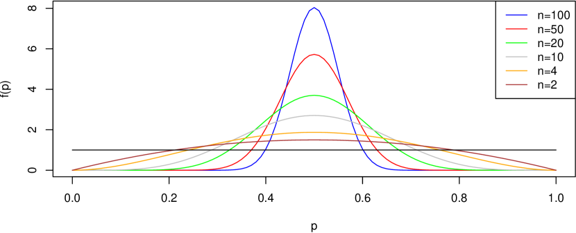
Figure 1: Probability density function of the white ball proportion $p$, having observed exactly 50% white balls in 2, 4, 10, 20, 50 and 100 extractions (the curves become in order narrower). The horizontal line represents the uniform prior.

We see that with the increasing number of extractions we get more and more confident that $p$ is around 0.5.

The most probable values of $p$ are those around $n_{W}/(n_{W}+n_{B})$, although the probability to have a white ball in a future observation has to take into account all possible compositions in a manner similar to that seen in Eq. (7), i.e.

$$P(\mbox{W}\,|\,{\mbox{\boldmath$E$}},B_{?},I) = \int_{0}^{1}\!p\,f(p\,|\,{\mbox{\boldmath$E$}},B_{?},I)\,dp\,.$$ (26)

In the r.h.s. of (26) we recognize the expected value of $p$, ‘barycenter’ of the probability density function. Therefore it follows that

$$P(\mbox{W}\,|\,{\mbox{\boldmath$E$}},B_{?},I) = \mbox{E}[p\,|\,{\mbox{\boldmath$E$}},B_{?},I]=\int_{0}^{1}\!p\,f(p\,|\,{\mbox{\boldmath$E$}},B_{?},I)\,dp\,.$$ (27)

The result of the integral (26) is

$$\int_{0}^{1}\!p\,f(p\,|\,{\mbox{\boldmath$E$}},B_{?},I)\,dp = \frac{n_{W}+1}{n_{W}+n_{B}+2}\,,$$ (28)

thus leading to the famous (although often misused!) Laplace rule of successions

$$P(\mbox{W}\,|\,{\mbox{\boldmath$E$}},B_{?},I)=\frac{n_{W}+1}{n_{W}+n_{B}+2}$$ (29)

and, by symmetry,

$$P(\mbox{B}\,|\,{\mbox{\boldmath$E$}},B_{?},I)=\frac{n_{B}+1}{n_{W}+n_{B}+2}\,.$$ (30)

Using Peirce numbers, we get

$$P(\mbox{B}\,|\,20\mbox{B},B_{?},I) = \frac{21}{22}=95.5\%$$ (31)

$$P(\mbox{B}\,|\,1010\mbox{B}\!+\!990\mbox{W},B_{?},I) = \frac{991}{2002}=50.4\%\,,$$ (32)

providing quite different degrees of belief, as it is intuitive and as it was clear to Peirce, who, by the way, uses Laplace rule of successions several times in Ref. [1].

4 Weights of evidence in favor of a black or white bean under the thimble

We have now all the tools to analyze Peirce’s bag of bean example, in which the ‘arguments’ did not regard the box composition, but the occurrence of a white or black bean in a future extraction (the fact that the bean was extracted at the beginning is irrelevant, as it has already been observed).

Since the bag is ‘large’ the proportion of white beans can be considered as a real number $p$ ranging between 0 and 1. Moreover, as implicitly assumed by Peirce (but this specific assumption is not strictly needed for the main conclusions of the paper), we judge that the value of $p$ could lie with equal probability in any small interval in the range between 0 and 1 (‘uniform prior’). Therefore we can use the results obtained in the previous section.

Let us now calculate the weight of evidence provided by the observation of black or white in favor of the occurrence of black or white. We need to calculate the Bayes factor that changes the odd ratio $P(\mbox{W}\,|\,{\mbox{\boldmath$E$}},B_{?},I)/P(\mbox{B}\,|\,{\mbox{\boldmath$E$}},B_{?},I)$ if we add a further observation $E_{n+1}$, schematically

$$\frac{P(\mbox{W}\,|\,{\mbox{\boldmath$E$}},B_{?},I)}{P(\mbox{B}\,|\,{\mbox{\boldmath$E$}},B_{?},I)} \rightarrow \frac{P(\mbox{W}\,|\,{\mbox{\boldmath$E$}},E_{n+1},B_{?},I)}{P(\mbox{B}\,|\,{\mbox{\boldmath$E$}},E_{n+1},B_{?},I)}\,.$$ (33)

This updating factor cannot be calculated directly in an easy way, but it can be nevertheless valuated indirectly by its definition (’final odds divided initial odds’). In fact, the evaluation of initial and final odds is very simple, just applying Laplace’s rule. For the former we have

$$O_{W,B}(n_{W},n_{B},I) = \frac{P(\mbox{W}\,|\,{\mbox{\boldmath$E$}},B_{?},I)}{P(\mbox{B}\,|\,{\mbox{\boldmath$E$}},B_{?},I)}=\frac{n_{W}+1}{n_{B}+1}\,.$$ (34)

The observation of a new white or of a new black changes this ratio in

$$O_{W,B}(n_{W}+1,n_{B},I) = \frac{(n_{W}+1)+1}{n_{B}+1}$$ (35)

$$O_{W,B}(n_{W},n_{B}+1,I) = \frac{n_{W}+1}{(n_{B}+1)+1}\,,$$ (36)

respectively. Dividing Eqs. (35) and (36) by (34) we get the updating factors of interest:

$$\tilde{O}_{W,B}(\mbox{W},n_{W},n_{B},I) = \frac{n_{W}+2}{n_{W}+1}$$ (37)

$$\tilde{O}_{W,B}(\mbox{B},n_{W},n_{B},I) = \frac{n_{B}+1}{n_{B}+2}\,.$$ (38)

Contrary to other usual Bayes factors, they depend on the previous amount of like-color balls already observed. [We can easily understand that they also depend on the priors on the box composition, and therefore Eqs. (37)-(38) are only valid for a uniform prior.]

Let us apply these formulae to Peirce’s example. The first observation of black yields an updating factor of $1/2$, or $\Delta$JL of $-0.30$; the second $2/3$, or $\Delta\mbox{JL}=-0.18$; the third $3/4$, or $\Delta\mbox{JL}=-0.12$; and so on. The updating factor produced by the 20th observation is only 20/21=0.952, which corresponds to the little weight of evidence $\Delta\mbox{JL}=-0.02$. The overall factor is 1/21=0.048 ($\Delta\mbox{JL}=-1.32$), which is also equal to the final odds (the two hypotheses were considered initially equally likely), from which a probability of 4.5% for white and 95.5% for black can be calculated.

If the 21-st extraction results, instead, in white, the new updating factor is 2 ($\Delta\mbox{JL}=0.30$), changing sizeable the overall updating factor, that becomes then $2/21$, or $\Delta\mbox{JL}=-1.02$, thus almost doubling the probability of white, that becomes then $8.7\%$. This is very interesting: the first time either color occurs it changes the odds by a factor of two in favor of that color ($|\Delta\mbox{JL}=0.30|$). A second observation of white gives an updating factor of $4/3$ ($\Delta\mbox{JL}=0.12$) and so on.

If we observe 1010 black and 990 white balls, the updating factor can be divided into the product of a factor given to white beans and a factor given to black ones, i.e. $\tilde{O}_{1,2}(990n_{W},1010n_{B},I)=\tilde{O}_{1,2}(990n_{W},I)\times\tilde{O}_{1,2}(1010n_{B},I)$, with

$$\tilde{O}_{1,2}(1010n_{B},I) = \frac{1}{2}\times\frac{2}{3}\times\frac{3}{4}\times\cdots\times\frac{1010}{1011}$$ (39)

$$\tilde{O}_{1,2}(990n_{W},I) = 2\times\frac{3}{2}\times\frac{4}{3}\times\cdots\times\frac{991}{990}\,.$$ (40)

In the product the first 990 factors of $\tilde{O}_{1,2}(1010n_{B},I)$ are simplified by $\tilde{O}_{1,2}(990n_{W},I)$ and the final result is

$$\tilde{O}_{1,2}(990n_{W},1010n_{B},I) = \frac{991}{992}\times\frac{992}{993}\times\cdots\times\frac{1010}{1011}=\frac{991}{1011}\,:$$ (41)

the 20 residual ‘arguments’ in favor of black are not the early ones (in which case the result would be equal to the observation of twenty black in a row) but the late ones, individually very small ($\Delta$JL about $-0.0004$ each). All together they provide a negligible weight of evidence in favor of black, with a combined $\Delta$JL of $-0.0087$, and the result of Eq. (32) is reobtained.

5 Conclusions

This example shows the danger of drawing quantitative conclusions from qualitative, intuitive considerations (an issue extensively discussed in Ref. [2]). Yes, each observation of black is ‘an argument’ in favor of the opinion that the bean ‘under the thimble’ is black. But the arguments do have the same strength and then the final ‘intensity of belief’ (to use a very interesting expression by Peirce) does not depend simply on the difference of their numbers in favor of either color.

References

-
[1]
C.S. Peirce, The Probability of Induction,
in Popular Science Monthly, Vol. 12, p. 705, 1878.
http://www.archive.org/stream/popscimonthly12yoummiss#page/715. -
[2]
G. D’Agostini, A defense of Columbo
(and of the use of Bayesian inference in forensics):
A multilevel introduction to probabilistic reasoning,
http://arxiv.org/abs/1003.2086. - [3] G. D’Agostini, Bayesian reasoning in data analysis – a critical introduction, World Scientific 2003.