The population of variable stars in M54 (NGC6715)

Abstract

We present new B, V and I CCD time-series photometry for 177 variable stars in a $13\arcmin\times 13\arcmin$ field centered on the globular cluster M54 (lying at the center of the Sagittarius dwarf spheroidal galaxy), 94 of which are newly identified variables. The total sample is composed of 2 anomalous Cepheids, 144 RR Lyrae stars (108 RR0 and 36 RR1), 3 SX Phoenicis, 7 eclipsing binaries (5 W UMA and 2 Algol binaries), 3 variables of uncertain classification and 18 long-period variables. The large majority of the RR Lyrae variables likely belong to M54. Ephemerides are provided for all the observed short-period variables. The pulsational properties of the M54 RR Lyrae variables are close to those of Oosterhoff I clusters, but a significant number of long-period ab type RR Lyrae are present. We use the observed properties of the RR Lyrae to estimate the reddening and the distance modulus of M54, E(B-V)=0.16 $\pm$ 0.02 and (m-M)₀=17.13 $\pm$ 0.11, respectively, in excellent agreement with the most recent estimates. The metallicity has been estimated for a subset of 47 RR Lyrae stars, with especially good quality light curves, from the Fourier parameters of the V light curve. The derived metallicity distribution has a symmetric bell shape, with a mean of $\langle[Fe/H]\rangle=-1.65$ and a standard deviation $\sigma=0.16$ dex. Seven stars have been identified as likely belonging to the Sagittarius galaxy, based on their too high or too low metallicity. This evidence, if confirmed, might suggest that old stars in this galaxy span a wide range of metallicities.

1 Introduction

The globular cluster M54 (NGC6715) is a special object under several aspects. In fact, it is quite massive ($\sim 2\times 10^{6}~{}M_{\sun}$, Pryor & Meylan 1993), it displays a complex Horizontal Branch (HB) morphology (extending up to the highest temperatures achievable by these stars; Rosenberg et al. 2004) and its stars present an intrinsic spread in Iron abundances (Carretta et al. 2010, C10 hereafter; see Bellazzini et al. 2008, hereafter B08, for previous studies and references). Moreover, it resides at the center of the Sagittarius dwarf spheroidal galaxy (Sgr dSph; Ibata, Gilmore & Irwin 1994), a satellite of the Milky Way that is currently disrupting under the tidal strain of the Galaxy (see, for example, Majewski et al. 2003). Several authors suggested the possibility that M54 could be the nucleus of Sgr (Bassino & Muzzio 1995; Sarajedini & Layden 1995). Later studies (Layden & Sarajedini 2000; Majewski et al. 2003; Monaco et al. 2005a), however, demonstrated that the metal-poor cluster ([Fe/H]$\simeq-1.55$; Brown, Wallerstein & Gonzalez 1999, C10) co-exists with a stellar nucleus made of metal rich stars of the Sgr galaxy ($\langle[Fe/H]\rangle\simeq-0.45$; B08 and references therein). A recent study based on accurate velocity and metallicity data (B08) strongly supports the idea that M54 formed independently, and plunged into the Sgr nucleus as a result of significant decay of its original orbit due to dynamical friction (Monaco et al. 2005b; see also C10 for independent support to this hypothesis).

In this context, RR Lyrae (RRL) variables can provide further insight into the nature of this stellar system, in addition to reliable estimates of the distance and foreground extinction. The first (photographic) survey for variable stars in M54 was performed by Rosino & Nobili (1959) who identified 82 variables. Their pioneering analysis was followed up and expanded by Layden & Sarajedini (2000; LS2000 hereafter), who considered the variables as part of their V,I CCD photometric study aimed at obtaining the colour-magnitude diagram (CMD) of M54 + Sgr field to derive the star formation history of the Sgr dSph galaxy. In that work LS2000 found 117 variable stars, 93 of which are candidate RRL stars. They analysed the best observed subset of RRL (67 stars) to obtain a distance modulus of $(m-M)_{0}=17.19\pm 0.12$ and E(V-I)=$0.18\pm 0.02$. On the basis of the pulsational properties of their sample of RRL, these authors classified M54 as an Oosterhoff type I cluster (Oosterhoff 1939; see Catelan 2009 for a recent review).

In this paper we present new BVI photometric data and discuss in detail the characteristics of the RRL stars of M54, that were presented in preliminary form by Cacciari, Bellazzini & Colucci (2002). In Sect. 2 we describe our data, the observations, the data reduction, the calibration procedure and the period search procedure. In Sect. 3 we present and briefly discuss the characteristics of the CMD resulting from our photometric data and present our sample of detected variables. In Sect. 4 we analyze the RRL pulsational properties and use them to estimate their membership to the M54 or Sgr stellar population. Sect. 5 presents the results of the Fourier analysis of the RRL light curves and metallicity estimates. The reddening and distance are derived in Sect. 6, and the properties of the other variables of our sample are briefly presented and discussed in Sect. 7. We summarize and discuss our results in Sect. 8. In Appendix A we comment on individual variables.

2 The data

2.1 Observations

The BVI photometric data presented in this paper were obtained on 13, 14 and 19 July 1999 at the ESO-Danish 1.54-m telescope in La Silla (Chile) using the 2k$\times$2k CCD of the Danish Faint Object Spectrograph and Camera (DFOSC). The images cover a $\simeq 13\arcmin\times 13\arcmin$ field of view roughly centered on M54, with a scale of 0.39 $\arcsec$/pixel. The BVI images were taken sequentially with exposure times of 360-900 sec in B, 150-600 sec in V, and 150-450 sec in I, depending on the atmospheric conditions. The average seeing during the three nights ranged between $1.9\arcsec$ and $2.5\arcsec$ (FWHM). In total, it was possible to obtain 54 B, 57 V and 52 I images.

2.2 Data reduction

The frames were overscan corrected, bias subtracted and flat fielded (using twilight sky flats) by means of the standard IRAF tasks.

The data reduction was performed using the ISIS package (Alard 2000), which is based on the method of image subtraction. ISIS is able to transform a series of images of the same field to (a) the same astrometric system, (b) the same flux scale, and (c) the same Point Spread Function (PSF), without flux losses. Once all the above transformations have been performed, the data reduction proceeds as follows:

1. A high signal-to-noise reference frame (per filter) is constructed, by stacking a suitable number of images; in the present case the reference frames were built by stacking 14 B, 15 V and 14 I frames.

2. Each individual image is subtracted from the reference frame; the squares of the images of the residuals are co-added into a single image where there are only the variable sources.

3. Variable stars are identified on the stacked images of the residuals and their positions are recorded.

4. The residual flux is measured on each single subtracted image at the position of the detected variables, using a PSF fitting routine. A light curve in units of flux difference is obtained for each variable.

5. Photometry of the reference frames is obtained independently (in our case using DoPHOT; Schechter, Mateo & Saha 1993) to provide the flux zero point to the light curves (and convert into a scale of magnitudes). In our case we transformed the instrumental magnitudes obtained with DoPHOT into absolute Johnson-Cousins magnitudes using several hundreds of stars in common with the photometry by LS2000 (for V and I) and by Rosenberg, Recio-Blanco & Garcia-Marin (2004) for B magnitudes.

The image-subtraction technique has proven very powerful in detecting even low amplitude variables in crowded fields, ensuring a higher accuracy in relative photometry with respect to traditional techniques (see e.g. Olech et al. 1999; Mochejska et al. 2004; Corwin et al. 2006; Greco et al. 2009; we refer to these papers also for further details on the technique). As an example, in Fig. 1 we show for comparison the V light curves of 3 RRL variables in M54 that were measured by LS2000 with traditional techniques (DoPHOT) and by us with ISIS: the higher quality of the new light curves is readily evident.

There are two additional features of the specific application of the method performed in the present case that deserve to be described:

• The images of a few bright foreground stars were saturated in our frames. In the process of image subtraction these sources left spurious residuals due to different degree of saturation in the different frames, blooming etc. This in turn led to the identification of large numbers of spurious variable sources in the surroundings of these saturated stars. To remove contaminants from the list of variables before obtaining their light curves, we masked the surroundings of heavily saturated stars. The dimension of the masked areas was decided case by case, by inspecting the stacked image of the residuals.

• DoPHOT automatically masks the regions surrounding (even moderately) saturated stars and/or sources for which the PSF fit does not reach convergency. For this reason there are variable stars for which we obtain a good differential flux light curve from ISIS but are not measured by DoPHOT on the reference image. Hence they lack a zero-point and their light curves cannot be transformed into a magnitude scale. For these stars we cannot measure an absolute amplitude, but we can obtain reliable periods and classify them on the basis of their periods, the shape of the light curve and the similarity of the differential flux amplitudes with calibrated variables.

Figure 1: Comparison between the light curves obtained in this wprk (ISIS reduction package) and by LS2000 (DoPHOT) for three common stars of M54.

2.3 Light curve analysis

For the period search, we used the Graphical Analyzer of Time Series (GrATiS) program (see Clementini et al. 2000 for details), which was run on the ISIS differential flux data. This code (developed by P. Montegriffo at the Osservatorio Astronomico di Bologna) employes two different algorithms: (1) a Lomb periodogram (Lomb 1976) and (2) a best fit of the data with a truncated Fourier series (Barning 1963). The adopted period search procedure performs the Lomb analysis on a wide period interval. The Fourier algorithm refines the period definition and find the best-fitting model. The r.m.s. of the observed points about the best fit model is taken as the error associated to the mean magnitudes. This value is reported along with the photometric data for each variable in Table 1.

2.4 Astrometry

The x,y coordinates in pixels have been transformed into J2000 Equatorial coordinates with a second order polynomial fitted to $\sim 2000$ stars in common with 2MASS (Skrutskie et al 2006), that were used as astrometric standards. The residuals of the adopted astrometric solution were $\la 0.14\arcsec$ r.m.s. in both RA and Dec.

3 Photometric results

3.1 Colour Magnitude Diagram

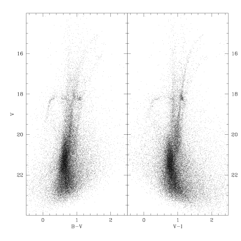
Figure 2: V-(B-V) (left panel) and V-(V-I) (right panel) CMDs of M54 and Sgr, based on the present data.

In Fig. 2 the V-(B-V) and V-(V-I) CMDs obtained with DoPHOT from the reference BVI images are shown. The CMD reaches a limiting magnitude of $V\sim 23$ sampling the population of M54 and Sgr down to $\sim$ 2 magnitudes below the cluster main sequence turn-off. The vertical plume of stars at $B-V(V-I)\ga 0.6(0.8)$ is composed by foreground/background Galactic main sequence stars at various distances along the line of sight. The steep and narrow Red Giant Branch (RGB) of M54 is clearly visible, bending from $B-V(V-I)\simeq 0.8(1.0)$ at $V\simeq 20$ to $B-V(V-I)\simeq 1.6(1.8)$ at $V\simeq 15$. The wider (and sparser) RGB of Sgr runs nearly parallel to the red of the M54 one. A well-defined blue HB (mostly associated to M54; see Monaco et al. 2004) and a well populated Red Clump (associated to Sgr) are also visible at V$\sim$18.2. A detailed discussion of the CMD is out of the scope of the present paper; we address the interested reader to papers more focused on the interpretation of the CMD (Sarajedini & Layden 1995; Monaco et al., 2003, 2004, and references therein). For a detailed analysis of the stellar content in the innermost region of the cluster, see the exquisite CMD obtained by Siegel et al. (2007) from Hubble Space Telescope data. For the purposes of the present analysis, it is important to recall that within the limiting radius of M54 ($r_{t}=6.3\arcmin$; see Ibata et al. 2009), the surface density of the cluster is nearly everywhere a factor of 7-8 larger than the Sgr metal-rich nucleus (B08). Moreover, the population of the Sgr nucleus is dominated by intermediate-age stars that are unlikely to evolve into RRL (Siegel et al. 2007 and references therein) producing a fraction of RRL which should be much lower than in M54 (Monaco et al. 2004). This is in agreement with Cseresnjes (2001), who estimated a density of 139 RR0 per square degree in the central region of Sgr, leading to about 6.5 RR0 in our 13 arcmin square field of view. Therefore, we conclude that the sample of RR Lyrae assembled in the present study must be dominated by members of M54.

3.2 The Variables

Our photometric search allowed us to identify 177 variable stars (94 new discoveries), significantly increasing the number (117) of variables identified by the previous studies of Rosino & Nobili (1959) and LS2000. The identification and photometric information are given in Table 1. In Fig. 3 the variables detected in this study are identified in the V-(B-V) CMD.

Among the 89 stars studied by LS2000: 2 (V23 and V91) were not identified in the present study because they lie out of our FoV; 4 (V25, V108, V111 and V112) were not identified because they were masked out during the variable detection phase (see Sect. 2.2); 4 (V86, V89, V90 and V95) were identified as variables but no light curve could be derived and one (V100) was found to be non variable. Of the variables reported in the former study of Rosino & Nobili (1959) 5 of them (V21, V26, V73, V79 and V81) were not identified, neither by us nor by LS2000, because no stars were detected at the locations indicated by Rosino & Nobili (1959) and 5 (V20, V22, V27, V53 and V72) were found to be non variable (as also found by LS2000). These stars are not listed in Table 1. Finally, 18 stars were identified and analysed using only internally calibrated photometry; they do appear in Table 1 but no photometric information is provided. The agreement between the light curves and the estimated periods between us and LS2000 is very good, in general. A few discordant cases are discussed in Appendix A.

For the 61 variable stars of the LS2000 sample for which we have calibrated photometry, we obtained light curves and derived the ephemerides using LS2000 photometric data in combination with ours to obtain a longer time baseline and more accurate results.

For the 94 newly identified variables (V118-V211) we derived the classification and the periods. We found: 51 RR0, 29 RR1, 3 SX Phoenicis, 3 W Uma (EW), one Algol binary (EA), 4 long period (LP) candidates (with no period determination) and 3 with uncertain classification (V145, V147 and V211) of which two (V147 and V211) might be eclipsing binaries (EB). From the present calibrated data we find no evidence of double-mode pulsation in any of the studied stars. For 58 of these stars, mostly located in the central region of M54, the photometry could not be externally calibrated for the reasons described in Sect. 2.2.

The light curves of a sample of newly discovered RRL and other variables are shown in Fig.s 4 and 5. The epoch photometry for all the variables with calibrated photometry is available in its entirety at the CDS.

In the following we will focus the analysis only on RR Lyrae stars; variables of other types will be briefly discussed in Sect. 7.

Figure 3: Expanded V-(B-V) CMD of M54. The detected variables are shown as: open circles (RR Lyrae stars), filled squares (Cepheids), asterisks (eclipsing binaries), filled triangles (SX Phoenicis) and open stars (uncertain classification).

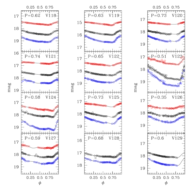
Figure 4: Light curves of a sample of newly discovered RR Lyrae variables of M54. Blue (lower), black (middle) and red (upper) data points indicate B,V and I magnitudes, respectively. The best fit models obtained with GrATIS are overplotted.

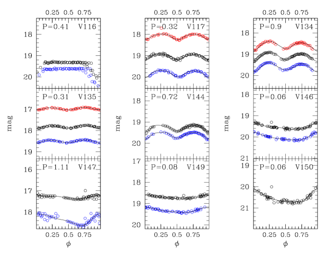
Figure 5: Same as Fig. 4 for other types of variables of M54.

Table 1: The RR Lyrae variable stars in the M54 field of view: a sample of the online catalog (the full catalog is available in the electronic version). Columns are: (1) Identification (ID) from Clement et al. (2001) and LS2000 up to V117, and from this paper for V118 to V221; (2) variable types: 0=Cepheid; 1=RR0; 2=RR1; 3=SX Phe; 4=LP; 5=EW; 6=EA; 7=Uncertain (3-4) RA and Dec coordinates. The epoch of the astrometric reference is J2000; (5) Pulsation period (6) Epoch of maximum light; (7-9) mean BVI magnitudes calculated as intensity averages over the pulsation cycle converted back to magnitudes; (10) r.m.s. of the observed V light curve points about the best fit model; (11-13) BVI amplitudes; (14-15) B-V and V-I colors at minimum light (phase interval 0.5-0.8); (16-17) mean $<B-V>$ and $<V-I>$ colors calculated as averages over one pulsation cycle of the best fit models; (18) Notes: Bl = possible Blazhko variability; b = possible blend; Cal = calibration problem; F = possible Galactic field member; Sgr = possible Sgr member; Ev = possible evolved.

ID	Ty	RA (J2000)	Dec (J2000)	Period	Epoch	$B$	$V$	$I$	rmsV	$A_{B}$	$A_{V}$	$A_{I}$	(B-V$)_{min}$	(V-I$)_{min}$	$<$B-V$>$	$<$V-I$>$	Note
n.		deg	deg	d	HJD
					2451370+
01	0	283.7906329	-30.4768056	1.3476492	2.11223	17.73	17.24	16.60	0.01	1.26	0.94	0.56	0.675	0.790	0.532	0.662
02	0	283.7621242	-30.4543426	1.0945410	2.65622	17.73	17.34	16.72	0.02	1.04	0.89	0.57	0.424	0.759	0.411	0.635
03	1	283.7591376	-30.4295744	0.5726301	9.60328	18.70	18.19	17.52	0.03	1.09	0.76	0.55	0.610	0.745	0.536	0.687
04	1	283.7454891	-30.3931179	0.4832307	9.75278	18.57	18.32	17.64	0.03	1.41	0.77	0.60	0.590	0.717	0.338	0.693	Bl
05	1	283.7218320	-30.4670001	0.5790976	9.70703	18.66	18.11	17.47	0.02	1.23	0.95	0.66	0.583	0.754	0.562	0.664
06	1	283.8307177	-30.5287519	0.5384199	3.51936	18.41	18.03	17.43	0.04	1.17	0.71	0.68	0.596	0.583	0.420	0.610	Bl
07	1	283.7810458	-30.5232817	0.5944093	4.57644	18.73	18.21	17.54	0.01	0.86	0.74	0.47	0.574	0.762	0.537	0.681
12	2	283.6919599	-30.5478954	0.3226390	9.30830	17.14	16.71	16.15	0.03	0.48	0.34	0.22	—–	—–	0.435	0.569	F
14	1	283.8410760	-30.4206737	0.4807214	3.04538	—–	—–	—–	—-	—-	—-	—-	—–	—–	—–	—–
15	1	283.8053859	-30.4962929	0.5868540	3.54588	18.69	18.21	17.53	0.02	0.95	0.93	0.61	0.493	0.800	0.481	0.704
28	1	283.7859926	-30.4341522	0.5088183	3.83630	18.48	18.08	17.51	0.05	1.40	1.18	0.78	0.518	0.734	0.432	0.614	Bl,Sgr
29	1	283.7226484	-30.4924474	0.5897109	2.90001	18.77	18.25	17.52	0.02	0.92	0.72	0.41	0.575	0.801	0.532	0.742
30	1	283.7645154	-30.4570863	0.5738690	9.65573	18.74	18.24	17.55	0.02	1.10	0.87	0.56	0.588	0.777	0.524	0.701
31	1	283.7323449	-30.4985297	0.6466228	3.56726	—–	18.18	17.43	0.02	—-	0.40	0.23	—–	0.802	—–	0.746
32	1	283.7063948	-30.4623137	0.5191334	3.85942	18.49	18.08	17.46	0.07	1.27	0.90	0.72	0.517	0.772	0.443	0.644	Bl
33	1	283.7890960	-30.5073081	0.4930339	3.51936	18.75	18.13	17.59	0.06	1.12	0.77	0.74	0.647	0.604	0.633	0.560	Bl
34	1	283.7473555	-30.5219780	0.5034071	3.83630	18.68	18.16	17.61	0.03	1.38	1.14	0.70	0.527	0.767	0.524	0.604
35	1	283.7377861	-30.4650676	0.5267239	9.78589	18.66	18.20	17.59	0.03	1.41	1.09	0.74	0.587	0.734	0.500	0.639
36	1	283.8053328	-30.4637899	0.5990345	9.66790	18.70	18.16	17.47	0.02	0.80	0.60	0.41	0.619	0.757	0.551	0.701
37	1	283.7784287	-30.4907654	0.6274528	3.77083	18.74	18.21	17.49	0.01	0.62	0.48	0.23	0.566	0.794	0.529	0.727
38	1	283.7424905	-30.4697269	0.6111295	9.64313	18.58	18.04	17.30	0.02	0.60	0.43	0.28	0.565	0.788	0.542	0.743
39	1	283.7323257	-30.4975579	0.5995711	3.77083	—–	18.19	17.53	0.02	—-	0.76	0.48	—–	0.755	—–	0.680
40	1	283.7483469	-30.5102175	0.5863672	2.66921	18.74	—–	17.51	—-	0.90	—-	0.50	—–	—–	—–	—–
41	1	283.8052158	-30.4654648	0.6176814	3.68530	18.77	18.15	17.43	0.05	0.97	1.04	0.61	0.594	0.870	0.613	0.752	Ev
42	2	283.7866761	-30.4629200	0.3264348	9.07901	—–	18.19	17.65	0.02	—-	0.49	0.31	—–	—–	—–	0.553
43	1	283.7150492	-30.4659484	0.5928533	4.64542	18.73	18.20	17.46	0.02	0.87	0.80	0.57	0.587	0.830	0.542	0.757	Bl
44	1	283.7688542	-30.5014846	0.6207049	9.49051	18.77	18.25	17.52	0.02	0.61	0.39	0.27	0.590	0.770	0.538	0.732
45	1	283.8036281	-30.5080007	0.4888223	3.47103	18.62	18.24	17.63	0.03	1.32	1.02	0.62	0.530	0.752	0.427	0.640
46	1	283.7530186	-30.4903405	0.6047506	4.52668	18.65	18.08	—–	0.02	0.64	0.56	—-	0.603	—–	0.581	—–	Sgr
47	1	283.7542761	-30.4532285	0.5069847	2.88684	18.62	18.22	17.61	0.02	0.44	0.70	0.41	0.332	0.670	0.397	0.618	Bl

4 Properties of the RR Lyrae stars

The sample of variables detected in our survey is mainly constituted by RRL stars, as expected from an old metal-poor globular cluster (GC). In this section we discuss the mebership of the various RRL, attempting to define a sample of M54 RRL as clean as possible from interlopers and/or stars with uncertain or possibly problematic data. Then, we will use the cleaned sample to analyze the pulsational properties of the cluster RRL.

4.1 The distribution in colour and magnitude

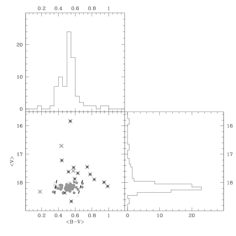
Figure 6: Colour-magnitude distribution of RR Lyrae stars in the V-(B-V) plane (bottom-left panel). RR0 and RR1 variables are marked with filled and open grey circles, respectively. Stars rejected from the M54 sample (see Sect. 4.1) are marked with black crosses. The two dashed lines indicate the edges of the instability strip (from Bono et al. 1995). The $<B-V>$ colour and $<V>$ magnitude distributions are shown in the upper-left and bottom-right panels, respectively.

Figure 7: The cumulative radial distribution of the RRL of M54 (solid line) compared with those of the BHB (dotted line) and red clump (dashed line) stars. The BHB and red clump stars are highlighted in the CMD (upper panel), for convenience.

We show in Fig. 6 the distribution in magnitude and colour of the RRL stars for which we obtained calibrated photometry. The magnitude histogram in the lower-right panel shows that the distribution is dominated by a strong and relatively narrow peak around $V\simeq 18.2$, clearly associated to the cluster population. The bulk of this population is well bracketed between the edges of the instability strip predicted by theoretical models (Bono, Caputo & Marconi 1995) for a 0.65 $M_{\odot}$ RRL star with Z=0.0004, overplotted to the CMD of Fig. 6. Here we assume $(m-M)_{0}=17.13$ and $E(B-V)=0.16$, according to the results of Sect. 6.1, below.

There are several stars that lie outside the M54 peak, both in magnitude and colour. There are 11 variables (9 RR0 and 2 RR1) having $\langle V\rangle<17.9$, clearly brighter than the bulk of the RRL population, i.e., in order of increasing magnitude, V119, V12, V128, V132, V93, V142, V65, V121, V75, V92, and V69. Assuming $M_{V}(RR)=0.6$ and $E(B-V)=0.16$ we can obtain rough estimates of the distances of these stars. V119 has $D\sim 9$ kpc, thus may be possibly located in the Galactic Bulge. The others range between $D\sim 13$ kpc and $D\sim 23$ kpc; while some of these are likely interlopers from the Galactic thick disc and/or halo, the faintest ones are more likely members of M54 (or Sgr dSph) that appear over-luminous because of blending with other sources and/or some unidentified problem in the photometry; in fact four of them (V92, V128, V132 and V142) lie in the most crowded region of our images, within $1\arcmin$ from the cluster center.

V55 (the faintest of the outliers, $D\sim 33$ kpc) is likely a genuine Galactic star in the background. Finally there are five stars that have at least one colour clearly outside the RRL window (V75, V123, V124, V133, V143; only V75 appears anomalous in both colours): this is likely due to a problem in the DoPHOT photometry of the reference frame in one of the three bands. V123, that appears rather normal from Fig. 6 has a very red V-I.

To keep our final sample of M54 RRL as clean and safe as possible, all the stars discussed above have been excluded from the analysis of the pulsational properties, in the following. The RRL of this clean sample (55 RR0 and 9 RR1) have $17.9<V<18.4$ mag and $0.3<B-V<0.7$. In Fig. 7 the cumulative radial distribution of the RRL in the clean sample is compared with those of the Blue HB stars (BHB; expected to be dominated by M54 population) and red clump stars. As expected, both the RRL and the BHB stars are significantly more concentrated than the red-clump stars. This indicates that the contamination by Galactic and/or Sgr variables should be minimal (see also Monaco et al. 2003).

In Fig. 8 the Zero Age Horizontal Branch (ZAHB) model (from Cariulo, Degl’Innocenti & Castellani 2004) for a population with metallicity $Z=0.0006$ and helium abundance $Y=0.23$ is overplotted to the $V-(B-V)$ CMD of M54. Two evolutionary tracks corresponding to mass values of $M=0.65~{}M_{\odot}$ and $M=0.70~{}M_{\odot}$ are overplotted. Absolute magnitudes have been converted to apparent ones adopting the reddening and distance modulus derived in Sect. 6 and 6.1. The ZAHB model fits quite well the lower envelope of the RRL distribution. Three stars are about 0.2 mag fainter than the average, namely V4, V118 and V130. The variable V4 is affected by the Blazhko effect and we have likely missed the maximum, as suggested by the unusually low V amplitude (0.71 mag) for its period (0.48 d). The other two stars have normal well defined light curves, and no metallicity estimates are available to check the origin of their unusual magnitude.

Figure 8: Colour-magnitude distribution of the HB area in the V-(B-V) plane. RR Lyrae stars are shown as open circles. The ZAHB model (solid line) for metallicity $Z=0.0006$ and helium abundance $Y=0.23$, and the evolutionary tracks (dashed lines) for the two stellar masses M=0.65 and 0.70 $M_{\odot}$ (from Cariulo et al. 2004) are overplotted.

4.2 Pulsational properties

If we consider the entire sample of RRL, including also those for which only internal calibrated photometry could be obtained (but excluding those flagged as non-member or problematic in the previous section), then we have 95 RR0 stars with $<P_{ab}>$ = 0.584d and 33 RR1 stars with $<P_{c}>$ = 0.351d. For comparison, the average values for Oosterhoff I type clusters are $<P_{ab}>$ = 0.559d and $<P_{c}>$ = 0.326d, while for Oosterhoff II type clusters they are $<P_{ab}>$ = 0.659d and $<P_{c}>$ = 0.368d (Smith 1995). The fraction of RR1 over the entire sample of RRL is 0.26, which is slightly higher than the typical fraction detected in Oosterhoff I clusters (0.22) and significantly smaller than the typical value (0.48) in Oosterhoff II clusters (Clement et al. 2001). This indicates that the entire sample of RRL stars detected in the M54 region has intermediate characteristics between the classical Oosterhoff types I and II, being much closer to Oosterhoff I. If we consider only the subset of stars that are most likely M54 members according to luminosity and metallicity criteria, as we discuss in Sect. 5, we find $<P_{ab}>$ = 0.600 d from 49 RR0 stars and $<P_{c}>$ = 0.347 d from 7 RR1 stars

In the middle panel of Fig. 9 the period-V amplitude diagram for the sample of RRL is shown. The mean loci of the unevolved RR0 and RR1 variables in the GGCs M3 (Oosterhoff I) and M92 (Oosterhoff II) are overplotted (from Cacciari, Corwin & Carney 2005). Taken at face value, the majority of the RR0 fall around the ridge line of M3 slightly on the side of smaller amplitudes or shorter periods. Some of these stars could well be unrecognised Blazhko variables observed during the low amplitude phase of the Blazhko modulation. Indeed, Blazhko effect has been clearly detected for 9 RRLs of our sample. According to previous studies (Smith 1995; Corwin & Carney 2001; Cacciari et al. 2005) as much as 30% of the total RRL population in several clusters is affected by Blazhko modulation. If the M54 population shares the same behaviour, then at least twice as many Blazhko RRL variables, whose anomaly could not be detected because of the short time coverage of our observations, are expected to exist in the studied sample . Within these uncertainties, the M54 data appear to be in good agreement with the mean relations derived for M3, albeit with a somewhat larger scatter (that may be due to the intrinsic metallicity spread of the cluster, see C10). In the bottom panel of Fig. 9 the period distribution of the RRL of M54 is compared with that of M3.

The apparent contadiction between the location in the P-Av diagram (slightly on the side of shorter periods) and the (longer) mean period of the M54 RRab stars with respect to M3 is an optical effect of the different amplitude distributions: while 44% of M3 RRab have amplitudes $A_{V}>1~{}mag$, this fraction is only 11% in M54. At least part of this difference might be due to the presence of a significant fraction of unrecognised Blazhko variables. As for the period distributions, which are not affected by the Blazhko stars, it is evident that the M54 and M3 RRL period distributions are different: the M3 distribution is skewed towards the short period end whereas in M54 it is wider and more symmetrical (bottom panel of Fig.9). This accounts for a longer mean RRab period in M54 ($\sim$0.60d) than in M3 ($\sim$0.56d).

One can also note a group of 8 stars with longer periods that seem to stand out from the main distribution . These stars are V41, V48, V76, V83, V120, V125, V137 and V140. This location in the period-amplitude diagram can be due to evolution off the ZAHB or to lower metallicity. In both cases the star is expected to be somewhat overluminous. Two of them (V125 and V137) are indeed brighter than the average by more than 0.1 mag and might be evolved, for the other 6 stars the luminosity is quite normal. The metallicity was estimated for 4 of these stars (V41, V48, V76 and V83) and falls within about 0.2 dex of the mean value except for V83 that is very metal-poor (see Sect. 5).

In conclusion M54 RRL show Oosterhoff I characteristics as far as the population ratio of fundamental/first overtone pulsators is concerned, while display average periods quite intermediate between the two types, mainly due to the presence of a significant number of long period RRL.

Figure 9: Upper panel: Period - $<V>$ distribution, cleaned of field contaminants, possible blends and photometric errors. Fundamental (RR0) and first overtone (RR1) pulsators are marked with filled and open circles, respectively. Blazhko stars are indicated as asterisks. The limiting magnitude of our selection criterion are marked with dashed lines. Middle panel: Period - V amplitude diagram for the RRL of M54. The symbols are the same as the upper panel. The mean loci of the unevolved RRL in M3 (solid line) and M92 (dashed line) are overplotted (from Cacciari et al. 2005). Lower panel: Period distributions for the RRL of M54 (grey histogram) and M3 (open histogram).

5 Metallicity estimates from Fourier analysis

It was shown that appropriate combinations of terms of a Fourier representation of RRL light curves, along with the periods, correlate with intrinsic parameters of the stars, such as metallicity, mass, luminosity and colours (Simon 1988; Clement, Jankulak & Simon 1992; Jurcsik & Kovacs 1996; Kovacs & Walker 2001; Morgan, Wahl & Wieckhorst 2007). Sandage (2004) interpreted the metallicity dependence of the Fourier components of RRL light curves as equivalent to the Oosterhoff-Arp-Preston period-metallicity effect. This can be found in both fundamental and first overtone pulsators, that we consider here separately.

However, in several cases (Jurcsik & Kovacs 1996; Pritzl et al. 2001; Nemec 2004; Cacciari et al 2005; Stetson, Catelan & Smith 2005) the coefficients as well as the range of validity of such relations have been discussed, often leading to different and conflicting results. Therefore, [Fe/H] estimates derived from the Fourier parameter $\phi_{31}$ should be used with caution, especially in the high metallicity regime. In the following we use these metallicites mainly to clean the sample of M54 RRL stars from possible members of Sgr, that would lie at the same distance but may stand out as significant outliers in the metallicity distribution.

To this purpose, we have decomposed the V light curves of all RRL variables of our sample in Fourier series of cosines.

5.1 RR1

Table 2: Fourier parameter $\phi_{31}$ (cosine series) and [Fe/H] for the RR1 variable stars. In column 5 the Notes indicate: * = excluded for its high/low magnitude (see Sect.4.1); ** = excluded from the analysis for its high/low metallicity (see Sect. 5.2).

ID	Period	$\phi_{31}$	$[Fe/H]_{ZW}$	Note
	(d)
V12	0.3226390	4.277	-1.01	*
V42	0.3264349	3.140	-1.73
V49	0.3312773	3.867	-1.40
V56	0.3676695	3.741	-1.81
V74	0.2889211	4.267	-0.49	**
V78	0.4019678	4.473	-1.72
V97	0.3367274	3.653	-1.58
V126	0.3516532	3.810	-1.65
V133	0.3648148	3.782	-1.77
V138	0.3116047	3.059	-1.62
V141	0.3339446	4.327	-1.13	**
V142	0.2978301	2.333	-1.79	*
V148	0.2670186	4.149	-0.19	**

The use of Fourier coefficients to characterise RR1 variables has been less extensive than that of the RR0 stars. The most recent critical analysis of this method has been presented by Morgan et al. (2007). We refer to this work for an extended discussion and references. According to these authors the metallicity of the RR1 stars can be estimated using the following relation:

$$[Fe/H]_{ZW}=52.466P^{2}-30.075P+0.131\phi_{31}^{2}+0.982\phi_{31}$$

$$-4.198P\phi_{31}+2.424~{}~{}~{}~{}~{}~{}~{}~{}~{}~{}~{}~{}~{}~{}~{}$$

where [Fe/H]_ZW is expressed in the Zinn & West (1984) metallicity scale, and the coefficient $\phi_{31}$ comes from Fourier light curve decomposition in series of cosines. The standard deviation of this relation, obtained from 106 stars, is 0.145 dex. The standard deviation of this relation, obtained from 106 RRc stars in 12 globular clusters, is 0.145 dex. The [Fe/H] values of the calibrating clusters are between approximately -1 and -2, so this relation likely gives poorer results at very high or very low metallicities.

Our sample contains 13 RR1 stars for which we have estimated the Fourier parameter $\phi_{31}$ and hence the metallicity with the above relation. The results are listed in Table 2. Two stars (V12 and V142) have been assigned to the Galactic field population based on their unusually bright V magnitude ($V<17.9$). Three more stars (V74, V141 and V148) have rather high metallicities suggesting that they may belong to the Sgr dSph population. The average metallicity of the 8 stars that are most likely M54 members is [Fe/H]= -1.66, with a standard deviation of 0.13 dex.

5.2 RR0

Figure 10: Metallicity distribution of the 30 RR0 variables with $D_{m}\leq 5$ and $17.9<V<18.4$. The range of the adopted selection for the bona fide sample of M54 are marked with dashed lines.

From the analysis of V light curves of 272 RR0 stars, Jurcsik & Kovacs (1996) and Jurcsik (1998) found a tight correlation (r.m.s. error of the fit 0.14 dex) between the metallicity of the variables and their $\phi_{31}$ (sine series) Fourier coefficents: $[Fe/H]=-5.038-5.394~{}P+1.345~{}\phi_{31}$. Based on the Layden (1994) [Fe/H] values of a large number of field RRab stars, Sandage (2004) recalibrated the above relation and obtained a lower zero-point by about -0.25 dex that is consistent with the Layden metallicity scale. This relation, that we use in the present analysis, is:

$$[Fe/H]_{L}=-5.492-5.666~{}P+1.413~{}\phi_{31}$$

where the r.m.s. error of the fit remains $\sim$ 0.14 dex. This new formulation gives values of metallicity that are in good agreement with those obtained from spectroscopy or other methods, as we comment later. Since we are also interested in differential estimates, to separate the M54 from the (Milky Way and Sgr) field populations, this method appears sufficiently adequate to identify at least the most obvious outliers. We corrected the values of our cosine series $\phi_{31}$ by +$\pi$ to report them to sine series decomposition, and applied the above relation to calculate the metallicity. The $D_{m}$ parameter (defined by Jurcsik & Kovacs 1996) represents a quality test on the regularity of the shape of the light curves, and hence on the reliability of the derived physical parameters. We considered as sufficiently reliable only stars with $D_{m}\leq 5$. The values of $\phi_{31}$ and [Fe/H]_L for these 38 RR0 stars are listed in Table 3. Blazhko stars should be excluded, unless observed at or near maximum Blazhko modulation amplitude with a good degree of confidence. In fact, at small-amplitude Blazhko phase the light curves are more likely distorted (even if Dm $\leq$5) and tend to overestimate the metallicity, whereas at large-amplitude Blazhko phase they are quite similar to regular pulsators (see Cacciari et al. 2005). Following these considerations, only V33 has been excluded from the sample. On the other hand, photometric blends or stars affected by calibration errors can still produce good metallicity estimates, as only the zeropoint of the photometric scale is incorrect. Seven variables with a reliable metallicity estimate have been associated to the foreground Galactic population because of their bright magnitudes.

The distribution of the remaining 30 RR0 variables with reliable metallicity estimates is shown in Fig. 10. As can be noted, the distribution has a prominent peak at $[Fe/H]\sim-1.6$ and the majority of RR0 variables have metallicities that range between $-2.2<[Fe/H]<-1.2$. A group of four variables (V28, V46, V63 and V123) form a secondary peak at $[Fe/H]\simeq-1.0$. One variable (V139) has a solar-like metallicity. Finally, two variables (V50 and V83) present a very low metallicity ($[Fe/H]<-2.2$). The membership of these 7 stars with metallicities outside the range $-2.2<[Fe/H]<-1.2$ is not clear cut. The extreme metallicity of V139, V50 and V83 strongly suggests a membership to Sgr dSph, whose metallicity distribution tails clearly reach values from $[Fe/H]\sim-2$ up to nearly solar (B08; Monaco et al 2005b; Bonifacio et al. 2006). In particular Cseresnjes (2001) found a very wide metallicity distribution also for the RRL of Sgr, with a mean of [Fe/H]=-1.6, a dispersion of $\sim 0.5$ dex, and a minor but significant population at $[Fe/H]\la$-2.0 dex. The membership of the four stars at $[Fe/H]\simeq-1.0$ is harder to establish, especially considering that M54 itself has been found (from spectroscopic analyses) to display a spread of $\sim 0.19$ dex (Da Costa & Armandroff 1995; B08; C10). To be conservative we decided to exclude also these four stars from our final sample.

The remaining 23 RR0 variables that are likely members of M54 have a mean metallicity [Fe/H]= -1.65 $\pm$ 0.18 dex. The mean metallicity of the M54 RR0 stars is in excellent agreement with the mean value found for the RR1 in Sect. 5.1. So we can assume that the RR1 and RR0 metallicity estimates can be dealt with jointly, and the mean value of the combined sample is [Fe/H]= -1.65, with a standard deviation of 0.16 dex, in good agreement with the spectroscopic estimates by Da Costa & Armandroff (1995), Brown et al. (1999), B08 and C10. The uncertainties on individual measures, on the reliability of the $\phi_{31}-[Fe/H]$ relations and the conservative selection described above prevent any conclusion about the intrinsic metallicity spread.

By rejecting those RRL with measured metallicities outside the range $-2.2<[Fe/H]<-1.2$ , in addition to the luminosity criteria described in Sect. 4.1, we end up with a sample of 49 RR0 and 7 RR1 variables, that will be used in the following sections to estimate the distance modulus and the reddening of M54.

In the following, we will refer to these stars as the bona-fide M54 sample.

Table 3: Fourier parameter $\phi_{31}$ (cosine series) and [Fe/H] values for the RR0 variable stars with Dm $<$5 in the M54 field of view. In column 5 the Notes indicate: * = excluded for its high/low magnitude (see Sect.4.1); ** = excluded from the analysis for its high/low metallicity (see Sect. 5.2).

ID	Period	$\phi_{31}$	[Fe/H]	Note
	(d)		L84
V3	0.5726301	1.880	-1.64
V5	0.5790976	1.702	-1.93
V7	0.5944093	1.956	-1.65
V15	0.5868540	1.906	-1.69
V28	0.5088183	2.030	-1.07	Blazhko, **
V29	0.5897109	2.115	-1.41
V30	0.5738690	1.994	-1.49
V32	0.5191334	1.521	-1.85	Blazhko
V33	0.4930339	1.894	-0.66:	Blazhko, low-ampl.
V34	0.5034071	1.786	-1.38
V35	0.5267239	1.573	-1.81
V41	0.6176814	2.202	-1.44
V43	0.5928533	2.020	-1.56	Blazhko
V45	0.4888223	1.404	-1.84
V46	0.6047506	2.629	-0.76	**
V48	0.6870139	2.262	-1.75
V50	0.5636133	1.258	-2.47	**
V55	0.4260544	2.154	-0.42	*
V58	0.5486673	1.797	-1.62
V61	0.6039009	2.165	-1.42
V63	0.5901396	2.361	-1.06	**
V65	0.5748202	2.045	-1.42	*
V67	0.5900106	1.896	-1.72
V69	0.6797878	2.006	-2.07	*
V75	0.5846341	1.907	-1.67	*
V76	0.7064914	2.378	-1.70
V77	0.5769039	1.867	-1.68
V82	0.5878700	2.020	-1.53
V83	0.5783485	1.398	-2.35	**
V85	0.5213111	1.381	-2.06
V92	0.4840892	1.557	-1.60	*
V93	0.5585378	1.780	-1.70	*
V96	0.5585253	1.883	-1.56
V119	0.6366165	2.356	-1.33	*
V123	0.5141767	2.112	-0.98	**
V124	0.5822650	1.812	-1.79
V129	0.6027318	2.060	-1.56
V139	0.4039767	2.337	-0.04	**

6 Reddening and Distance

Our large sample of RRL allows us to determine the reddening to M54 with good accuracy. We consider two approaches to estimate the reddening, using the colours of the RR0 variables at minimum light (i.e. averaged over the phase interval 0.5-0.8):

• Based on a recalibration of the original relation by Sturch (1966), Walker (1998) proposed a relation linking $(B-V)_{min}$ and reddening $E(B-V)$:

  $$E(B-V)=(B-V)_{min}-0.24~{}P-0.056~{}[Fe/H]-0.356$$

  Applying this relation to the sample of bona-fide RR0 variables of M54 we find $E(B-V)=0.17\pm 0.02$ if we adopt an average metallicity $[Fe/H]=-1.65$ (see Sect. 5) and $E(B-V)=0.16\pm 0.06$ if we adopt for each star the metallicity estimated through the $\phi_{31}-[Fe/H]$ relation defined in Sect. 5.2

• From the analysis of a sample of field RR0 stars Mateo et al. (1995) proposed a constant value of $(V-I)_{0,min}=0.58$ for RR0 stars, independent on metallicity and period. By using our sample of bona-fide M54 RR0 stars we find $<(V-I)_{min}>=0.78\pm 0.03$ which translates into $E(V-I)=0.20\pm 0.03$, and hence $E(B-V)=0.16\pm 0.03$ using the relation E(B-V)=0.8 E(V-I)(Dean, Warren & Cousin 1978).

Summarizing the above results, we estimate an average value of $E(B-V)=0.16\pm 0.02$. This estimate is in very good agreement with that provided by the extinction map by Schlegel, Finkbeiner & Davis (1998, $E(B-V)=0.15\pm 0.02$), and with the results by LS2000 from a similar analysis of RRL stars ($E(V-I)=0.18\pm 0.02$).

6.1 Distance determination

The distance to M54 has been estimated from the mean characteristics of the bona fide sample using the absolute visual magnitude M_V that can be derived from the luminosity-metallicity relation

$$M_{V}=0.214~{}[Fe/H]+0.885$$

(Clementini et al. 2003) where the adopted slope 0.214 appears to be supported by the most accurate studies of field RRL stars in the Milky Way (Fernley et al. 1998; Chaboyer 1999), in the Large Magellanic Cloud (LMC; Gratton et al. 2004) and GCs in M31 (Rich et al. 2005). The zero-point of such a relation has been set to be consistent with the mean dereddened V magnitude of the RR0 variables observed in the LMC by Clementini et al. (2003) ($<V_{0}>=19.064$) assuming a distance modulus of $(m-M)_{0}=18.50$ (Freedman et al. 2001).

We use the mean metallicity $[Fe/H]=-1.65\pm 0.16$ dex (derived from the subset described in Sect. 5) to estimate $<M_{V}>=0.53\pm 0.05$ mag from the above equation, and the mean V magnitude $<V>=18.16\pm 0.07$ mag (derived from the stars that have been included in the bona fide sample). Therefore, assuming $A_{V}/E(B-V)=3.1$ (Savage & Mathis 1979) and E(B-V)=0.16 $\pm$ 0.02 (see Sect. 6) we estimate a distance modulus to M54 $(m-M)_{0}=17.13\pm 0.11$, which translates into a distance to M54 of $d=26.7\pm 1.1$ kpc. As a sanity check, we estimate the distance modulus also adopting the individual Fourier metallicities listed in Tables 2 and 3 for the smaller sample of 30+7 RR0+RR1 variables, and we obtain $(m-M)_{0}=17.11\pm 0.13$.

The above estimates are in excellent agreement with those derived by Monaco et al. (2004; $(m-M)_{0}=17.10\pm 0.15$), and by LS2000, once their estimate is corrected using the most recent metallicity estimates ($(m-M)_{0}=17.13\pm 0.09$; see Monaco et al. 2004). A significantly smaller distance ($(m-M)_{0}=16.97\pm 0.07$) has been derived by Kunder & Chaboyer (2009) on the basis of the analysis of differential distance modulus of a sample of Sgr RRL with respect to a sample of RRL belonging to the Galactic bulge. These authors adopt a different luminosity-metallicity relation (from Bono, Caputo & Di Criscienzo 2007), and their sample is affected by larger amount of extinction (E(B-V)=0.36), lying in fields at lower Galactic latitude, from $4\deg$ to $10\deg$ apart from M54. Moreover, the derived distance clearly depends on the assumed distance to the Galactic Bulge. Finally, a lower distance in that wing of the Sgr dSph may be a real effect of the three dimesional orientation of the galaxy major axis. All these factors can contribute to account for the difference between their distance estimate and our results (as well as those by LS2000 and Monaco et al. 2004; see the latter paper for a detailed discussion and references on previous distance estimates).

7 Other variables

Figure 11: V-(V-I) CMD of M54 and Sgr. The locations of the 18 candidates LPV are marked with open circles.

Apart from the RRL, a number of other variables have been found in the present survey.

Variables V1 and V2 are Cepheids already discovered by Rosino & Nobili (1959) and classified by LS2000 as a population II and an anomalous cepheid, respectively. Their magnitudes are consistent with those predicted by the period-luminosity relation of Nemec, Nemec & Lutz (1994) and are located at 3.2 and 3.5 arcmin from the cluster center, respectively. On the basis of these considerations they should be likely members of M54 (or Sgr dSph).

Among eclipsing binaries, stars V116 and V195 are Algol binaries (EA), whereas V147 and V211 are suspected EB types. Five variables (namely V99, V117, V134, V135, and V144) are probably W UMa (EW). By applying the period-colour-V luminosity relations by Rucinski (2000) we estimated the distance moduli of these stars. Among these 5 stars, only V134 and V144 have distance moduli $17.3<(m-M)_{0}<17.5$ which are compatible with that of M54 estimated in Sect. 6.1, being probable cluster members.

We found 3 SX Phoenicis variables (V146, V149 and V150) with periods in the range $0.06~{}d<P<0.08~{}d$. Adopting the period-luminosity relation by Poretti et al. (2008) we estimated the distances for these stars. V146 and V149 are significantly less distant than M54 ($\Delta~{}(m-M)_{0}\sim 0.6-1.0$ mag) and are likely foreground Galactic variables. The distance modulus of V150 is compatible (within 0.3 mag) with that of M54 and could be a cluster or Sgr member.

Finally, we identified 18 candidate long-period variables (LPV). Four of them (V153, V154, V155 and V156) are new discoveries. They are located in the CMD close to the tip of the RGB at colours $(V-I)>1.4$ (see Fig. 11). Most of them are located far from the RGB ridge line of M54, on the expected locus of late M giants of Sgr, being likely associated to Sgr.

Of course, the short time coverage of our observations does not allow us to establish their pulsation periods and their average magnitudes and colours are uncertain.

8 Discussion and Conclusions

We presented a survey of variable stars in a 13 arcmin square field of view centred on the GC M54 using deep multi-epoch observations collected with the ESO-Danish 1.54m telescope. From this analysis we detected 177 variables, 94 of them never observed before. We provide the ephemerides for the entire sample of variables (except for 18 long-period candidates), and the epoch-photometry and light curves for the large subset of variables with calibrated photometry.

The period-amplitude diagram of the RRL of M54 and the relative fraction of RR1 variables indicate that this cluster shares some of the properties of Oosterhoff I clusters (as already found by LS2000), but contains a larger number of long-period variables. The average period of its RR0 and RR1 stars are indeed slightly larger than typical Oosterhoff I cluster values, even if significantly smaller than Oosterhoff II.

Accurate estimates of the cluster reddening ($E(B-V)=0.16\pm 0.02$) and distance modulus ($(m-M)_{0}=17.13\pm 0.11$) were also derived, in excellent agreement with previous estimates in literature.

The metallicity distribution of the RRL, derived through the Fourier parameter $\phi_{31}$, shows a clear peak at the metallicity of M54 ($[Fe/H]\sim-1.65\pm 0.16$ dex) and a few stars with a significantly different metallicity (outside the range $-2.2<[Fe/H]<-1.2$), likely associated with the population of the Sgr dSph. The presence of a extended blue HB (reaching the instability strip) associated with the Sgr galaxy has been already discovered by Monaco et al. (2003). We note that the presence of RRL stars as metal-rich as $[Fe/H]\ga-0.8$ (see also Cseresjnes 2001), if confirmed, would indicate that Sgr was able to reach such relatively high metallicity at a very early epoch ($\ga 10$ Gyr ago). Unfortunately, the small number of stars belonging to this group and the large uncertainties in the metallicities do not allow a firm conclusion on this issue until spectroscopic confirmation is obtained.

Appendix A Comments on individual variables

• V4: V magnitude $\sim$ 0.2 mag fainter than the bulk M54 RRL population. Affected by the Blazhko effect, the maximum has likely been missed, as suggested by the unusually low V amplitude (0.71 mag) for its period (0.48 d).

• V12: we have derived a more accurate period (P=0.322639), which fits both our data and LS2000 data, whereas LS2000 estimate (P=0.31985) produces out-of-phase curves. The star is bright and its Fourier metallicity is [Fe/H]=-1.01, this suggests that it may belong to the Galactic field population.

• V14: classified as RR0 with P=0.70489 by LS2000, this star shows a good light curve (internal photometry only) with P=0.4807214 in clear disagreement also with Rosino & Nobili (1959) determination.

• V28: Metal-rich ([Fe/H]=-1.07). Normal V magnitude and position in the Av-logP diagram. Possible Sgr member.

• V41: Slightly shifted in the Av-logP plane towards long periods. Normal magnitude. Fourier metallicity [Fe/H]= -1.44.

• V46: Metal-rich ([Fe/H]=-0.76). Normal V magnitude and position in the Av-logP diagram. Possible Sgr member.

• V48: Shifted in the Av-logP plane towards long periods. Normal magnitude. Fourier metallicity [Fe/H]= -1.75. Possibly belonging to Sgr.

• V50: Metal-poor ([Fe/H]=-2.47). Normal V magnitude and position in the Av-logP diagram. Possible Sgr member.

• V55: faint magnitude, likely background Galactic field star. This is confirmed by its location in the P-Av diagram, much to the short-period side of the main distribution for the M54 stars, also supported by the metallicity obtained from the Fourier parameters ([Fe/H]=-0.43).

• V63: Metal-rich ([Fe/H]=-1.06). Normal V magnitude and position in the Av-logP diagram. Possible Sgr member.

• V65: bright. Fourier metallicity [Fe/H]= -1.42 . Normal position in the Av-logP diagram, likely field star.

• V69: bright. Fourier metallicity [Fe/H]= -2.07 . Shifted toward long periods in the Av-logP diagram, field star or evolved.

• V74: Metal-rich ([Fe/H]=-0.49). Normal V magnitude and position in the Av-logP diagram. Possible evolved or Sgr member.

• V75: unusually red colours (B-V = 0.78; V-I = 0.45). Slightly brighter than average. Fourier metallicity [Fe/H]=-1.67 dex. Normal position in the Av-logP diagram. Photometric calibration error (See Sect. 4.1).

• V76: Shifted in the Av-logP plane towards long periods. Normal magnitude. Fourier metallicity [Fe/H]= -1.70. Possibly belonging to Sgr.

• V83: Metal-poor ([Fe/H]=-2.35). Normal V magnitude. Slightly shifted in the Av-logP plane towards long periods. Possible Sgr member.

• V92: slightly brighter than average and redder than expected from its period. Fourier metallicity [Fe/H]=-1.60 dex. Located within central 1 arcmin, possibly a blend.

• V93: bright. Fourier metallicity [Fe/H]=-1.71 dex. Likely field star.

• V118: V magnitude $\sim$ 0.2 mag fainter than the bulk M54 RRL population. Normal location in the Av-logP plane.

• V119: very bright. Fourier metallicity [Fe/H]=-1.33 dex. Foreground star (Galactic population).

• V120: Shifted in the Av-logP plane towards long periods. Normal magnitude. Possibly belonging to Sgr.

• V121: bright. Likely field star.

• V123: unusually red V-I colour (V-I = 1.00) in spite of normal B-V (B-V=0.47). Fourier metallicity [Fe/H]=-0.98. Photometric calibration error (See Sect. 4.1).

• V124: unusually red B-V colour (B-V = 0.94) in spite of normal V-I (V-I=0.50). Fourier metallicity [Fe/H]=-1.79. Photometric calibration error (See Sect. 4.1).

• V125: Shifted in the Av-logP plane towards long periods. V magnitude $\sim$ 0.1 brighter than the bulk M54 RRL population. Probably evolved variable.

• V128: bright. Normal location in the Av-logP plane. Located within the central 1 arcmin, possibly a blend with a field “blue plume” star.

• V130: V magnitude $\sim$ 0.2 mag fainter than the bulk M54 RRL population. Normal location in the Av-logP plane.

• V132 bright, and redder than the assumed red edge of the instability strip. Normal location in the Av-logP plane. Located within the central 1 arcmin, possibly a blend with a “red clump” star.

• V133: unusually blue B-V colour (B-V = 0.18). Photometric calibration error (See Sect. 4.1).

• V137: Shifted in the Av-logP plane towards long periods. V magnitude $\sim$ 0.1 brighter than the bulk M54 RRL population. Probably evolved variable.

• V139: the period-amplitude values locate the star among the RR1 variables, however the light curve shows the typical shape of a fundamental pulsator. The metallicity obtained from the Fourier parameters is [Fe/H]=-0.04. Therefore this star likely belongs to the metal-rich ($\sim$ solar metallicity) tail of the Sgr field stellar population.

• V140: Shifted in the Av-logP plane towards long periods. Normal magnitude. Possibly belonging to Sgr.

• V141: Metal-rich ([Fe/H]=-1.13). Normal V magnitude and position in the Av-logP diagram. Possible Sgr member.

• V142: bright. Located within central 1 arcmin, possibly a blend.

• V143: unusually red colour (B-V = 0.99). Photometric calibration error (See Sect. 4.1).

• V145: the classification of this star is highly uncertain. The data from the first two night would be compatible with a RR1, those from the third night are not. The period and the complete light curve may suggest a classification as a RS CVn variable, with a possible alternative period of 1.053375 days. Its position in the CMD (straight on the cluster HB) may indicate a similarity with the case of the superposition of two RRL discussed by Corwin & Carney (1998).

• V147: period and the B light curve are quite typical of RR0 stars, with an amplitude of $\simeq 0.6$ mag. The V light curve does not seem compatible with this interpretation, probably due to an error in the photometric zero point (from DoPHOT photometry of the V reference frame). For this reason we flag this variable as uncertain.

• V211: uncertain classification.

References

- Alard (2000) Alard C., 2000, A&AS, 144, 363
- Barning (1963) Barning F. J. M., 1963, BAN, 17, 22
- Bassino & Muzzio (1995) Bassino L.P., Muzzio J.C., 1995, The Observatory, 115, 256
- Bellazzini et al. (2008) Bellazzini M., Ibata R.A., Chapman S.C., et al. 2008, AJ, 136, 1147 (B08)
- Bonifacio et al. (2006) Bonifacio P., Zaggia S., Sbordone L., et al. 2006, in Chemical Abundances and Mixing in stars in the Milky Way and its Satellites, ed. S. Randich & L. Pasquini, Berlin:Springer, p. 232
- Bono et al. (2007) Bono G., Caputo F., Di Criscienzo M., 2007, A&A, 476, 779
- Bono et al. (1995) Bono G., Caputo F., Marconi M., 1995, AJ, 110, 2365
- Brown et al. (1999) Brown J. A., Wallerstein G., Gonzalez G., 1999, AJ, 118, 1245
- Cacciari et al. (2002) Cacciari C., Bellazzini M., Colucci S., 2002, Extragalactic Star Clusters, 207, 168
- Cacciari et al. (2005) Cacciari C., Corwin T. M., Carney B. W., 2005, AJ, 129, 267
- Cariulo et al. (2004) Cariulo P., Degl’Innocenti S., Castellani V., 2004, A&A, 421, 1121
- Carretta et al. (2010) Carretta E., Bragaglia A., Gratton R., et al., 2010, ApJ, in press (ArXiv:1002.1963; C10)
- Catelan (2009) Catelan, M. 2009, Ap&SS, 320, 261
- Chaboyer (1999) Chaboyer B., 1999, Post-Hipparcos cosmic candles, 237, 111
- Clement et al. (1992) Clement C. M., Jankulak M., Simon N. R., 1992, ApJ, 395, 192
- Clement et al. (2001) Clement C. M., Muzzin A., Dufton Q., et al., 2001, AJ, 122, 2587
- Clementini et al. (2000) Clementini G., Di Tomaso S., Di Fabrizio L., et al., 2000, AJ, 120, 2054
- Clementini et al. (2003) Clementini G., Gratton R., Bragaglia A., Carretta E., Di Fabrizio L., Maio M., 2003, AJ, 125, 1309
- Corwin & Carney (1998) Corwin T. M., Carney B. W., 1998, Information Bulletin on Variable Stars, 4547, 1
- Corwin & Carney (2001) Corwin T. M., Carney B. W. 2001, AJ, 122, 3183
- Corwin et al. (2006) Corwin, T.M., et al., 2006, AJ, 132, 1014
- Cseresnjes (2001) Cseresnjes P., 2001, A&A, 375, 909
- Da Costa & Armandroff (1995) Da Costa G. S., Armandroff T. E., 1995, AJ, 109, 2533
- Dean et al. (1978) Dean J. F., Warren P. R., Cousins A. W. J., 1978, MNRAS, 183, 569
- Fernley et al. (1998) Fernley J., Skillen I., Carney B. W., Cacciari C., Janes K., 1998, MNRAS, 293, L61
- Freedman et al. (2001) Freedman W. L., Madore B. F., Gibson B. K., et al., 2001, ApJ, 553, 47
- Gratton et al. (2004) Gratton R. G., Bragaglia A., Clementini G., Carretta E., Di Fabrizio L., Maio M., Taribello E., 2004, A&A, 421, 937
- Greco et al. (2009) Greco C., Clementni G, Catelan M., et al., 2009, ApJ, 701, 1323
- Ibata et al. (1994) Ibata R. A., Gilmore G., Irwin M. J., 1994, Nature, 370, 194
- Ibata et al. (2009) Ibata R., Bellazzini M., Chapman S. C., et al., 2009, ApJ, 699, L169
- Jurcsik (1998) Jurcsik J., 1998, A&A, 333, 571
- Jurcsik & Kovacs (1996) Jurcsik J., Kovacs G., 1996, A&A, 312, 111
- Kovács & Walker (2001) Kovács G., Walker A. R., 2001, A&A, 374, 264
- Kunder & Chaboyer (2009) Kunder A., Chaboyer B., 2009, AJ, 137, 4478
- Layden (1994) Layden A. C., 1994, AJ, 108, 1016
- Layden & sarajedini (2000) Layden A.C., Sarajedini A. 2000, AJ, 119, 1760 (LS2000)
- Lomb (1976) Lomb N. R., 1976, Ap&SS, 39, 447
- Majewski et al. (1993) Majewski S.R., Skruskie M.F., Weinberg A.D., Ostheimer J.C., 2003, ApJ, 599, 1082
- Mateo et al. (1995) Mateo M., Kubiak M., Szymanski M., Kaluzny J., Krzeminski W., Udalski A., 1995, AJ, 110, 1141
- Mochejska et al. (2004) Mochejska, B.J., 2004, AJ, 128, 312
- Monaco et al. (2003) Monaco L., Bellazzini M., Ferraro F. R., Pancino E., 2003, ApJ, 597, L25
- Monaco et al. (2004) Monaco L., Bellazzini M., Ferraro F. R., Pancino E., 2004, MNRAS, 353, 874
- Monaco et al. (2005a) Monaco L., Bellazzini M., Ferraro F.R, Pancino E., 2005a, MNRAS, 356, 1396
- Monaco et al. (2005b) Monaco, L., Bellazzini M., Bonifacio P., et al., 2005b, A&A, 441, 141
- Morgan, Wahl & Wieckhorst (2007) Morgan S.M., Wahl J.N., Wieckhorst R.M., 2007, MNRAS, 374, 1421
- Nemec (2004) Nemec J. M., 2004, AJ, 127, 2185
- Nemec et al. (1994) Nemec J. M., Nemec A. F. L., Lutz T. E., 1994, AJ, 108, 222
- Olech et al. (1999) Olech A., Woźniak P. R., Alard C., Kaluzny J., Thompson I. B., 1999, MNRAS, 310, 759
- Oosterhoff (1939) Oosterhoff P.Th., 1939, Observatory, 62, 104
- Poretti et al. (2008) Poretti E., Clementini G., Held E. V., et al., 2008, ApJ, 685, 947
- Pritzl et al. (2001) Pritzl B. J., Smith H. A., Catelan M., Sweigart A. V., 2001, AJ, 122, 2600
- Pryor & Meylan (1993) Pryor, C. & Meylan, G. 1993, in Structure and Dynamics of Globular Clusters, ASP Conf. Ser. 50, ed. S. Djorgovsky & G. Meylan (San Francisco, CA: ASP), 357
- Rich et al. (2005) Rich R. M., Corsi C. E., Cacciari C., Federici L., Fusi Pecci F., Djorgovski S. G., Freedman W. L., 2005, AJ, 129, 2670
- Rosenberg et al. (2004) Rosenberg A., Recio-Blanco A., García-Marín M., 2004, ApJ, 603, 135
- Rosino & Nobili (1959) Rosino L., Nobili F., 1959, Asiago Contrib., 97, 1
- Rucinski (2000) Rucinski S. M., 2000, AJ, 120, 319
- Sandage (2004) Sandage A., 2004, AJ, 128, 858
- Sarajedini & Layden (1995) Sarajedini A., Layden A.C., 1995, AJ, 109, 1086
- Savage & Mathis (1979) Savage B. D., Mathis J. S., 1979, ARA&A, 17, 73
- Schechter et al. (1993) Schechter P., Mateo M., Saha A. 1993, PASP, 105, 1342
- Schlegel et al. (1998) Schlegel D. J., Finkbeiner D. P., Davis M., 1998, ApJ, 500, 525
- Siegel et al. (2007) Siegel M.H., Dotter A., Majewski S.R., et al 2007, ApJ, 667, L57
- Simon (1988) Simon N. R., 1988, ApJ, 328, 747
- Skrutskie et al. (2006) Skrutskie M.F., Cutri R. M., Stiening R., et al., 2006, AJ, 131, 1163
- Smith (1995) Smith H. A., 1995, in ”RR Lyrae”, Cambridge Astrophysics Series, Cambridge, New York, Cambridge University Press
- Stetson et al. (2005) Stetson P. B., Catelan M., Smith H. A., 2005, PASP, 117, 1325
- Sturch (1966) Sturch C., 1966, ApJ, 143, 774
- Walker (1998) Walker A. R., 1998, AJ, 116, 220
- Zinn & West (1984) Zinn R., West M. J., 1984, ApJS, 55, 45