Scaling limits of Markov branching trees with applications to Galton–Watson and random unordered trees

Abstract

We consider a family of random trees satisfying a Markov branching property. Roughly, this property says that the subtrees above some given height are independent with a law that depends only on their total size, the latter being either the number of leaves or vertices. Such families are parameterized by sequences of distributions on partitions of the integers that determine how the size of a tree is distributed in its different subtrees. Under some natural assumption on these distributions, stipulating that “macroscopic” splitting events are rare, we show that Markov branching trees admit the so-called self-similar fragmentation trees as scaling limits in the Gromov–Hausdorff–Prokhorov topology.

The main application of these results is that the scaling limit of random uniform unordered trees is the Brownian continuum random tree. This extends a result by Marckert–Miermont and fully proves a conjecture by Aldous. We also recover, and occasionally extend, results on scaling limits of consistent Markov branching models and known convergence results of Galton–Watson trees toward the Brownian and stable continuum random trees.

T1Supported in part by ANR-08-BLAN-0190 and ANR-08-BLAN-0220-01.

and

1 Introduction and main results

The goal of this paper is to discuss the scaling limits of a model of random trees satisfying a simple Markovian branching property that was considered in different forms in Devroye , Aldous96 , BrDeMcLdlS , HMPW06 . Markov branching trees are natural models of random trees defined in terms of discrete fragmentation processes. The laws of these trees are indexed by an integer $n$ giving the “size” of the tree, which leads us to consider two distinct (but related) models, in which the sizes are, respectively, the number of leaves and the number of vertices. We first provide a slightly informal description of our results.

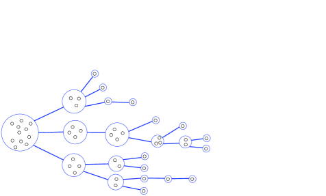
Figure 1: A sample tree $T_{11}$. The first splitting arises with probability $q_{11}(4,4,3)$.

Let $q=(q_{n},n\geq 1)$ be a family of probability distributions, respectively, on the set $\mathcal{P}_{n}$ of partitions of the integer $n$, that is, of nonincreasing integer sequences with sum $n$. We assume that $q_{n}$ does not assign mass $1$ to the trivial partition $(n)$

$$q_{n}((n))<1\qquad\mbox{for every }n\geq 1.$$

In order that this makes sense for $n=1$, we add an extra “empty partition” $\varnothing$ to $\mathcal{P}_{1}$.

One constructs a random rooted tree with $n$ leaves according to the following procedure. Start from a collection of $n$ indistinguishable balls, and with probability $q_{n}(\lambda_{1},\ldots,\lambda_{p})$, split the collection into $p$ sub-collections with $\lambda_{1},\ldots,\lambda_{p}$ balls. Note that there is a chance $q_{n}((n))<1$ that the collection remains unchanged during this step of the procedure. Then, re-iterate the splitting operation independently for each sub-collection using this time the probability distributions $q_{\lambda_{1}},\ldots,q_{\lambda_{p}}$. If a sub-collection consists of a single ball, it can remain single with probability $q_{1}((1))$ or get wiped out with probability $q_{1}(\varnothing)$. We continue the procedure until all the balls are wiped out. There is a natural genealogy associated with this process, which is a tree with $n$ leaves consisting in the $n$ isolated balls just before they are wiped out, and rooted at the initial collection of $n$ balls. See Figure 1 for an illustration. We let $\mathsf{P}^{q}_{n}$ be the law of this tree.

This construction can be seen as the most general form of splitting trees of Broutin et al. BrDeMcLdlS , and was referred to as trees having the so-called Markov branching property in HMPW06 . There is also a variant of this procedure that constructs a random tree with $n$ vertices rather than $n$ leaves. This one does not need the hypothesis $q_{n}((n))<1$ for $n\geq 1$, and in fact we only assume $q_{1}((1))=1$ for consistency of the description to follow. Informally, starting from a collection of $n$ balls, we first remove a ball, split the $n-1$ remaining balls in sub-collections with $\lambda_{1},\ldots,\lambda_{p}$ balls with probability $q_{n-1}((\lambda_{1},\ldots,\lambda_{p}))$, and iterate independently on sub-collections until no ball remains. We let $\mathsf{Q}^{q}_{n}$ be the law of the random tree associated to this procedure.

While most papers so far have been focusing on families of trees having more structure, such as a consistency property when $n$ varies Aldous96 , HMPW06 , Devroye (with the notable exception of Broutin et al. BrDeMcLdlS ), the main goal of the present work is to study the geometry of trees with laws $\mathsf{P}^{q}_{n}$ or $\mathsf{Q}^{q}_{n}$ as $n\to\infty$ in a very general situation. The main assumption that we make is that, as $n\to\infty$,

• “macroscopic” splitting events of the form $n\to(ns_{1},ns_{2},\ldots)\in\mathcal{P}_{n}$ for a nonincreasing sequence $\mathbf{s}=(s_{1},s_{2},\ldots)$ with sum $1$ and such that $s_{1}<1-\varepsilon$, for some $\varepsilon\in(0,1)$, are rare events, occurring with probability of order $n^{-\gamma}\nu_{\varepsilon}(\mathrm{d}\mathbf{s})$ for some $\gamma>0$, for some finite “intensity” measure $\nu_{\varepsilon}$.

Note that the measures $\nu_{\varepsilon}$ should satisfy a consistency property as $\varepsilon$ varies, and as $\varepsilon$ goes to $0$, $\nu_{\varepsilon}$ should increase to a possibly infinite measure $\nu$ on the set of nonincreasing sequences with sum $1$. This means that splitting events that only remove tiny parts from a large collection of balls are allowed to remain more frequent than the order $n^{-\gamma}$. Under this assumption, formalized in hypothesis (H) below, we show in Theorem 5 that a tree $T_{n}$ with law $\mathsf{P}^{q}_{n}$, considered as a metric space by viewing its edges as being real segments of lengths of order $n^{-\gamma}$, converges in distribution toward a limiting structure $\mathcal{T}_{\gamma,\nu}$, the so-called self-similar fragmentation tree of HM04 ,

$$\frac{1}{n^{\gamma}}T_{n}\longrightarrow\mathcal{T}_{\gamma,\nu}.$$

When $\gamma\in(0,1)$, a similar result (Theorem 6) holds when $T_{n}$ has distribution $\mathsf{Q}^{q}_{n}$.

The limiting tree $\mathcal{T}_{\gamma,\nu}$ can be seen as the genealogical tree of a continuous model for mass splitting, in some sense analogous to the Markov branching property described above. The above convergence holds in distribution in a space of measured metric spaces, endowed with the so-called Gromov–Hausdorff–Prokhorov topology. This result contrasts with the situation of BrDeMcLdlS , where it is assumed that macroscopic splitting events occur at every step of the construction. In that case, the height of $T_{n}$ is of order $\log n$, and no interesting scaling limit exists for the tree. A key step in our study will be to use the results from HaMi09 , where scaling limits of nonincreasing Markov chains were considered: such Markov chains are indeed obtained by considering the successive sizes of collections containing a particular marked ball when going up in the tree $T_{n}$.

This general statement allows us to recover, and sometimes improve, many results of HMPW06 , HPW , PiWi08 , CFW dealing specifically with Markov branching trees. It also applies to models of random trees that are not a priori directly connected to our study. In particular, we recover the results of Aldous AldousCRTIII and Duquesne duq02 showing that the so-called Brownian and stable trees AldousCRTI , LeGallLeJan , dlg02 , dlg05 are universal limits for conditioned Galton–Watson trees.

More notably, our results entail that uniform unordered trees with $n$ vertices, in which each vertex has at most $m\in[2,\infty]$ children, admit the Brownian continuum random tree as a scaling limit. This was conjectured by Aldous AldousCRTII and proved in MaMi09 in the particular case $m=2$ of a binary branching, using completely different methods from the present paper. The difficulty of handling such families of random trees comes from the fact that they have no “nice” probabilistic representations, using, for instance, branching processes or growth models. As a matter of fact, uniform random unordered trees do not even have the Markov branching property, but it turns out to be “almost” the case, in a sense that will be explained below.

The rest of this section is devoted to a detailed formalization of our results.

Index of notation

Throughout the paper, we use the notation

$$\mathbb{N}=\{1,2,3,\ldots\},\qquad\mathbb{Z}_{+}=\{0\}\cup\mathbb{N},\qquad[n]=\{1,2,\ldots,n\},\qquad n\in\mathbb{N}.$$

The random variables appearing in this paper are either canonical or defined on some probability space $(\Omega,\mathcal{F},\mathbb{P})$.

$\mathbbl{t}$	plane tree, page 1.1
$\mathsf{t}$	unordered tree, page 1.1
$\mathsf{T}_{n}$	set of trees with $n$ vertices, page 1.1
$\mathsf{T}^{\partial}_{n}$	set of trees with $n$ leaves, page 1.1
$p(\lambda)$	number of parts of a partition $\lambda$, page 1.2
$\mathcal{P}_{n}$	set of partitions of $n$, page 1.2
$m_{j}(\lambda)$	multiplicity of parts of $\lambda$ equal to $j$, page 1.2
$\mathsf{P}^{q}_{n}$	distributions of Markov branching trees indexed by leaves, page 1
$\mathsf{Q}^{q}_{n}$	distributions of Markov branching trees indexed by vertices, page 1.2.2
$T_{n}$	tree with distribution $\mathsf{P}^{q}_{n}$ or $\mathsf{Q}^{q}_{n}$, page 1
$d_{\mathrm{GH}}$	pointed Gromov–Hausdorff distance, page 1.3
$d_{\mathrm{GHP}}$	pointed Gromov–Hausdorff–Prokhorov distance, page 1.3
$\mathscr{T}$	set of isometry classes of compact rooted $\mathbb{R}$-trees, page 1.3.2

$\mathscr{T}_{\mathrm{w}}$	set of isometry classes of compact rooted measured $\mathbb{R}$-trees, page 1.3.2
$\mathcal{S}^{\downarrow}$	set of partitions of a unit mass, page 1.4
$\mathcal{T}_{\gamma,\nu}$	$(\gamma,\nu)$-fragmentation tree, page 4
$\mathsf{T}^{(m)}$	set of trees with $n$ vertices and at most $m$ children per vertex, page 2.2
$\mathcal{P}_{B}$	set of partitions of $B\subseteq\mathbb{N}$, page 3.1.1
$\mathcal{P}$	set of partitions with variable size, page 3.1.3
$\theta$	tree with edge-lengths, page 3.2.1
$\bolds{\Theta}$	set of trees with edge-lengths, page 3.2.1
$\mathcal{T}(\theta)$	$\mathbb{R}$-tree associated to $\theta$, page 3.2.1
$\mathcal{T}(\mathsf{t})$	$\mathbb{R}$-tree associated to a tree $\mathsf{t}$ with edge-lengths 1, page 3.2.1
$D^{\pi}_{B}$	death time of the block $B$ in the process $\pi$, page 3.2.2
$\theta(\pi(\cdot),B)$	tree with edge-lengths associated with a partition-valued process, page 3.2.2
$p_{B}(\pi)$	exchangeable distribution on partitions of $B$ associated with $q_{n}$, page 23

1.1 Discrete trees

We briefly introduce some formalism for trees. Set $\mathbb{N}^{0}=\{\varnothing\}$, and let

$$\mathcal{U}=\bigcup_{n\geq 0}\mathbb{N}^{n}.$$

For $u=(u_{1},\ldots,u_{n})\in\mathcal{U}$, we denote by $|u|=n$ the length of $u$, also called the height of $u$. If $u=(u_{1},\ldots,u_{n})$ with $n\geq 1$, we let $\mathrm{pr}(u)=(u_{1},\ldots,u_{n-1})$, and for $i\geq 1$, we let $ui=(u_{1},\ldots,u_{n},i)$. More generally, for $u=(u_{1},\ldots,u_{n})$ and $v=(v_{1},\ldots,v_{m})$ in $\mathcal{U}$, we let $uv=(u_{1},\ldots,u_{n},v_{1},\ldots,v_{m})$ be their concatenation. For $A\subset\mathcal{U}$ and $u\in\mathcal{U}$, we let $uA=\{uv\dvtx v\in A\}$, and simply let $iA=(i)A$ for $i\in\mathbb{N}$. We say that $u$ is a prefix of $v$ if $v\in u\mathcal{U}$, and write $u\preceq v$, defining a partial order on $\mathcal{U}$.

A plane tree is a nonempty, finite subset $\mathbbl{t}\subset\mathcal{U}$ (whose elements are called vertices), such that:

• if $u\in\mathbbl{t}$ with $|u|\geq 1$, then $\mathrm{pr}(u)\in\mathbbl{t}$;

• if $u\in\mathbbl{t}$, then there exists a number $c_{u}(\mathbbl{t})\in\mathbb{Z}_{+}$ (the number of children of $u$) such that $ui\in\mathbbl{t}$ if and only if $1\leq i\leq c_{u}(\mathbbl{t})$.

Let $\partial\mathbbl{t}=\{u\in\mathbbl{t}\dvtx c_{u}(\mathbbl{t})=0\}$ be the set of leaves of $\mathbbl{t}$. If $\mathbbl{t}^{(1)},\ldots,\mathbbl{t}^{(k)}$ are plane trees, we can define a new plane tree by

$$\bigl{\langle}\mathbbl{t}^{(1)},\ldots,\mathbbl{t}^{(k)}\bigr{\rangle}=\{\varnothing\}\cup\bigcup_{i=1}^{k}i\mathbbl{t}^{(i)}.$$

A plane tree has a natural graphical representation, in which every $u\in\mathbbl{t}$ is a vertex, joined to its $c_{u}(\mathbbl{t})$ children by as many edges. But $\mathbbl{t}$ carries more information than the graph, as it has a natural order structure. In this work, we will not be interested in this order, and we present one way to get rid of this unwanted structure. Let $\mathbbl{t}$ be a plane tree, and $\bolds{\sigma}=(\sigma_{u},u\in\mathbbl{t})$ be a sequence of permutations, respectively, $\sigma_{u}\in\mathfrak{S}_{c_{u}(\mathbbl{t})}$. For $u=(u_{1},\ldots,u_{n})\in\mathbbl{t}$, let

$$\bolds{\sigma}(u)=\bigl{(}\sigma_{\varnothing}(u_{1}),\sigma_{(u_{1})}(u_{2}),\sigma_{(u_{1},u_{2})}(u_{3}),\ldots,\sigma_{(u_{1},\ldots,u_{n-1})}(u_{n})\bigr{)}$$

and $\bolds{\sigma}(\varnothing)=\varnothing$. Then the set $\bolds{\sigma}(\mathbbl{t})=\{\bolds{\sigma}(u)\dvtx u\in\mathbbl{t}\}$ is a plane tree, obtained intuitively by shuffling the set of children of $u$ in $\mathbbl{t}$ according to the permutation $\sigma_{u}$. We say that $\mathbbl{t},\mathbbl{t}^{\prime}$ are equivalent if there exists some $\bolds{\sigma}$ such that $\bolds{\sigma}(\mathbbl{t})=\mathbbl{t}^{\prime}$. Equivalence classes of plane trees will be called (rooted) unordered trees, or simply trees as opposed to plane trees, and denoted by lowercase letter $\mathsf{t}$’s. They are sometimes called (rooted) Pólya trees in the literature drmota09 .

Given a tree $\mathsf{t}$, we will freely adapt some notation from plane trees when dealing with quantities that do not depend on particular plane representatives. For instance, $\#\mathsf{t},\#\partial\mathsf{t}$ will denote the number of vertices and leaves of $\mathsf{t}$, while $\varnothing,c_{\varnothing}(\mathsf{t})$ will denote the root of $\mathsf{t}$ and its degree.

We let $\mathsf{T}$ be the set of trees, and for $n\geq 1$,

$$\mathsf{T}^{\partial}_{n}=\{\mathsf{t}\in\mathsf{T}\dvtx\#\partial\mathsf{t}=n\},\qquad\mathsf{T}_{n}=\{\mathsf{t}\in\mathsf{T}\dvtx\#\mathsf{t}=n\}$$

be the set of trees with $n$ leaves, respectively, $n$ vertices. The class of $\{\varnothing\}$ is the vertex tree $\bullet\in\mathsf{T}_{1}=\mathsf{T}^{\partial}_{1}$.

Heuristically, the information carried in a tree is its graph structure, with a distinguished “root” vertex corresponding to $\varnothing$, and considered up to root-preserving graph isomorphisms—it is not embedded in any space, and its vertices are unlabeled.

It is a simple exercise to see that if $\mathsf{t}^{(i)},1\leq i\leq k$, are trees, and $\mathbbl{t}^{(i)}$ is a choice of a plane representative of $\mathsf{t}^{(i)}$ for each $i$, then the class of $\langle\mathbbl{t}^{(i)},1\leq i\leq k\rangle$ does not depend on the particular choice for $\mathbbl{t}^{(i)}$. We denote this common class by $\langle\mathsf{t}^{(i)},1\leq i\leq k\rangle$. Note that $j(\mathsf{t}):=\langle\mathsf{t}\rangle$ can be seen as the tree $\mathsf{t}$ whose root has been attached to a new root by an edge, and similarly $j^{l}(\mathsf{t})$, for $l\geq 0$, is the tree $\mathsf{t}$ whose root has been attached to a new root by a string of $l$ edges. For instance, $j^{l}(\bullet)$ is the line-tree consisting of a string with length $l$, rooted at one of its ends. Finally, for trees $\mathsf{t}^{(1)},\ldots,\mathsf{t}^{(k)}$ and $l\geq 1$ we let

$$\bigl{\langle}\mathsf{t}^{(1)},\ldots,\mathsf{t}^{(k)}\bigr{\rangle}_{l}=j^{l}\bigl{(}\bigl{\langle}\mathsf{t}^{(1)},\ldots,\mathsf{t}^{(k)}\bigr{\rangle}\bigr{)},$$

so $j^{l}(\bullet)=\langle\bullet\rangle_{l}$ with this notation.

1.2 Markov branching trees

A partition of an integer $n\geq 1$ is a sequence of integers $\lambda=(\lambda_{1},\ldots,\lambda_{p})$ with $\lambda_{1}\geq\cdots\geq\lambda_{p}\geq 1$ and $\lambda_{1}+\cdots+\lambda_{p}=n$. The number $p=p(\lambda)$ is called the number of parts of the partition $\lambda$, and the partition is called nontrivial if $p(\lambda)\geq 2$. We let $\mathcal{P}_{n}$ be the set of partitions of the integer $n$. We also add an extra element $\varnothing$ to $\mathcal{P}_{1}$, so that $\mathcal{P}_{1}=\{(1),\varnothing\}$.

If $(c_{1},c_{2},\ldots)$ is a finite or infinite sequence of nonnegative integers with finite sum and $j\geq 1$, we define

$$m_{j}(c_{1},c_{2},\ldots)=\#\{i\dvtx c_{i}=j\},$$

the multiplicity of terms of $c_{1},c_{2},\ldots$ that are equal to $j$. In particular, if $\lambda\in\mathcal{P}_{n}$, $m_{j}(\lambda)$ is the multiplicity of parts of $\lambda$ equal to $j$.

By convention, it is sometimes convenient to set $\lambda_{i}=0$ for $i>p(\lambda)$, and to identify the sequence $\lambda$ with the infinite sequence $(\lambda_{i},i\geq 1)$. Such identifications will be implicit when needed.

1.2.1 Markov branching trees with a prescribed number of leaves

In this paragraph, the size of a tree $\mathsf{t}\in\mathsf{T}$ is going to be the number $\#\partial\mathsf{t}$ of its leaves.

Let $q=(q_{n},n\geq 1)$ be a sequence of probability distributions, respectively, on $\mathcal{P}_{n}$,

$$q_{n}=\bigl{(}q_{n}(\lambda),\lambda\in\mathcal{P}_{n}\bigr{)},\qquad\sum_{\lambda\in\mathcal{P}_{n}}q_{n}(\lambda)=1,$$

such that

$$q_{n}((n))<1,\qquad n\geq 1.$$ (1)

Consider a family of probability distributions $\mathsf{P}^{q}_{n},n\geq 1$, on $\mathsf{T}^{\partial}_{n}$, respectively, such that: [(1)]

$\mathsf{P}^{q}_{1}$ is the law of the line-tree $\langle\bullet\rangle_{G}$, where $G$ has a geometric distribution given by

$$\mathbb{P}(G=k)=q_{1}(\varnothing)\bigl{(}1-q_{1}(\varnothing)\bigr{)}^{k},\qquad k\geq 0;$$

for $n\geq 2$, $\mathsf{P}^{q}_{n}$ is the law of

$$\bigl{\langle}T^{(i)},1\leq i\leq p(\Lambda)\bigr{\rangle},$$

where $\Lambda$ has distribution $q_{n}$, and conditionally on the latter, the trees $T^{(i)},1\leq i\leq p(\Lambda)$, are independent with distributions $\mathsf{P}^{q}_{\Lambda_{i}}$, respectively. Alternatively, for $n\geq 2$, $\mathsf{P}^{q}_{n}$ is the law of $\langle T^{(i)},1\leq i\leq p(\Lambda)\rangle_{G}$ where $G$ is independent of $\Lambda$ and geometric with

$$\mathbb{P}(G=k)=\bigl{(}1-q_{n}((n))\bigr{)}q_{n}((n))^{k},\qquad k\geq 0,$$

and conditionally on $\Lambda$, which has law $q_{n}(\cdot|\mathcal{P}_{n}\setminus\{(n)\})$, the trees $T^{(1)},\ldots,\break T^{(p(\Lambda))}$ are independent with distributions $\mathsf{P}_{\Lambda_{i}}$, respectively. A simple induction argument shows that there exists a unique family $\mathsf{P}^{q}_{n},n\geq 1$, satisfying properties 1 and 2 above.

A family of random trees $T_{n},n\geq 1$, with respective distributions $\mathsf{P}^{q}_{n},n\geq 1$, is called a Markov branching family. The law of the tree $T_{n}$ introduced in the beginning of the Introduction to describe the genealogy of splitting collections of $n$ balls is $\mathsf{P}^{q}_{n}$.

1.2.2 Markov branching trees with a prescribed number of vertices

We now consider the following variant of the above construction, in which the size of a tree $\mathsf{t}$ is the number of its vertices. For every $n\geq 1$, let again $q_{n}$ be a probability distribution on $\mathcal{P}_{n}$. We do not assume (1), rather, we make the sole assumption that $q_{1}((1))=1$. For every $n\geq 1$, we construct inductively a family of random trees $T_{n}$, respectively, in the set $\mathsf{T}_{n}$ of trees with $n$ vertices, by assuming that for $\lambda=(\lambda_{1},\ldots,\lambda_{p})\in\mathcal{P}_{n-1}$, with probability $q_{n-1}(\lambda)$, the $n-1$ vertices distinct from the root vertex are dispatched in $p$ subtrees with $\lambda_{1}\geq\cdots\geq\lambda_{p}$ vertices, and that, given these sizes, the $p$ subtrees are independent with same distribution as $T_{\lambda_{1}},\ldots,T_{\lambda_{p}}$, respectively.

Formally: [(1)]

let $\mathsf{Q}^{q}_{1}$ be the law of $\bullet$;

for $n\geq 1$, let $\mathsf{Q}^{q}_{n+1}$ be the law of

$$\bigl{\langle}T^{(i)},1\leq i\leq p(\Lambda)\bigr{\rangle},$$

where $\Lambda$ has distribution $q_{n}$, and conditionally on the latter, the trees $T^{(i)},1\leq i\leq p(\Lambda)$, are independent with distributions $\mathsf{Q}^{q}_{\Lambda_{i}}$, respectively. By induction, these two properties determine the laws $\mathsf{Q}_{n}^{q},n\geq 1$, uniquely.

The construction is very similar to the previous one, and can in fact be seen as a special case, after a simple transformation on the tree; see Section 4.5 below.

1.3 Topologies on metric spaces

The main goal of the present work is to study scaling limits of trees with distributions $\mathsf{P}^{q}_{n},\mathsf{Q}^{q}_{n}$, as $n$ becomes large. For this purpose, we need to consider a topological “space of trees” in which such limits can be taken, and define the limiting objects.

A rooted metric space is a triple $(X,d,\rho)$, where $(X,d)$ is a metric space and $\rho\in X$ is a distinguished point, called the root. We say that two rooted spaces $(X,\rho,d),(X^{\prime},\rho^{\prime},d^{\prime})$ are isometry-equivalent if there exists a bijective isometry from $X$ onto $X$ that sends $\rho$ to $\rho^{\prime}$.

A measured, rooted metric space is a 4-tuple $(X,d,\rho,\mu)$, where $(X,d,\rho)$ is a rooted metric space and $\mu$ is a Borel probability measure on $X$. Two measured, rooted spaces $(X,d,\rho,\mu)$ and $(X,d^{\prime},\rho^{\prime},\mu^{\prime})$ are isometry-equivalent if there exists a root-preserving, bijective isometry $\phi$ from $(X,d,\rho)$ to $(X,d^{\prime},\rho^{\prime})$ such that the push-forward of $\mu$ by $\phi$ is $\mu^{\prime}$. In the sequel we will almost always identify two isometry-equivalent (rooted, measured) spaces, and will often use the shorthand notation $X$ for the isometry class of a rooted space or a measured, rooted space, in a way that should be clear from the context. Also, if $X$ is such a space and $a>0$, then we denote by $aX$ the space in which the distance function is multiplied by $a$.

We denote by $\mathscr{M}$ the set of equivalence classes of compact rooted spaces, and by $\mathscr{M}_{\mathrm{w}}$ the set of equivalence classes of compact measured rooted spaces.

It is well known (this is an easy extension of the results of EPW ) that $\mathscr{M}$ is a Polish space when endowed with the so-called rooted Gromov–Hausdorff distance $d_{\mathrm{GH}}$, where by definition the distance $d_{\mathrm{GH}}((X,d,\rho),(X^{\prime},d^{\prime},\rho^{\prime}))$ is equal to the infimum of the quantities

$$\operatorname{dist}(\phi(\rho),\phi^{\prime}(\rho^{\prime}))\vee\operatorname{dist}_{\mathrm{H}}(\phi(X),\phi^{\prime}(X^{\prime})),$$

where $\phi,\phi^{\prime}$ are isometries from $X,X^{\prime}$ into a common metric space $(M,\operatorname{dist})$, and where $\operatorname{dist}_{\mathrm{H}}$ is the Hausdorff distance between compact subsets of $(M,\operatorname{dist})$. It is elementary that this distance does not depend on particular choices in the equivalence classes of $(X,d,\rho)$ and $(X^{\prime},d^{\prime},\rho^{\prime})$. We endow $\mathscr{M}$ with the associated Borel $\sigma$-algebra. Of course, $d_{\mathrm{GH}}$ satisfies a homogeneity property, $d_{\mathrm{GH}}(aX,aX^{\prime})=ad_{\mathrm{GH}}(X,X^{\prime})$ for $a>0$.

We also need to define a distance on $\mathscr{M}_{\mathrm{w}}$, that is in some sense compatible with the Gromov–Hausdorff distance. Several complete distances can be constructed, and we use a variation of the Gromov–Hausdorff–Prokhorov distance used in miermont09 . The induced topology is the same as that introduced earlier in EW . The reader should bear in mind that the topology used in the present paper involves a little extension of the two previous references, since we are interested in rooted spaces. We let $d_{\mathrm{GHP}}((X,d,\rho,\mu),(X^{\prime},d^{\prime},\rho^{\prime},\mu^{\prime}))$ be the infimum of the quantities

$$\operatorname{dist}(\phi(\rho),\phi^{\prime}(\rho^{\prime}))\vee\operatorname{dist}_{\mathrm{H}}(\phi(X),\phi^{\prime}(X^{\prime}))\vee\operatorname{dist}_{\mathrm{P}}(\phi_{*}\mu,\phi^{\prime}_{*}\mu^{\prime}),$$

where again $\phi,\phi^{\prime}$ are isometries from $X,X^{\prime}$ into a common space $(M,\operatorname{dist})$, $\phi_{*}\mu,\phi^{\prime}_{*}\mu^{\prime}$ are the push-forward of $\mu,\mu^{\prime}$ by $\phi,\phi^{\prime}$ and $\operatorname{dist}_{\mathrm{P}}$ is the Prokhorov distance between Borel probability measures on $M$ (EK , Chapter 3),

$$\operatorname{dist}_{\mathrm{P}}(m,m^{\prime})=\inf\{\varepsilon>0\dvtx m(C)\leq m^{\prime}(C^{\varepsilon})+\varepsilon\mbox{ for every }C\subset M\mbox{ closed}\},$$

where $C^{\varepsilon}=\{x\in M\dvtx\inf_{y\in C}\operatorname{dist}(x,y)<\varepsilon\}$ is the $\varepsilon$-thickening of $C$. A simple adaptation of the results of EW and Section 6 in miermont09 (in order to take into account the particular role of the distinguished point $\rho$) shows the following:

Proposition 1.

The function $d_{\mathrm{GHP}}$ is a distance on $\mathscr{M}_{\mathrm{w}}$ that makes it complete and separable.

This distance is called the rooted Gromov–Hausdorff–Prokhorov distance. One must be careful that contrary to $d_{\mathrm{GH}}$, this distance is not homogeneous: $d_{\mathrm{GHP}}(aX,aX^{\prime})$ is in general different from $ad_{\mathrm{GHP}}(X,X^{\prime})$, because only the distances, not the measures, are multiplied in $aX,aX^{\prime}$.

1.3.1 Trees viewed as metric spaces

A plane tree $\mathbbl{t}$ can be naturally seen as a metric space by endowing $\mathbbl{t}$ with the graph distance between vertices. Namely,

$$d_{\mathrm{gr}}(u,v)=|u|+|v|-2|u\wedge v|,\qquad u,v\in\mathbbl{t},$$

where $u\wedge v$ is the longest prefix common to $u,v$. This coincides with the number of edges on the only simple path going from $u$ to $v$. The space $(\mathbbl{t},d_{\mathrm{gr}})$ is naturally rooted at $\varnothing$. We can put two natural probability measures on $\mathbbl{t}$, the uniform measures on the leaves or on the vertices

$$\mu_{\partial\mathbbl{t}}=\frac{1}{\#\partial\mathbbl{t}}\sum_{u\in\partial\mathbbl{t}}\delta_{\{u\}},\qquad\mu{t}=\frac{1}{\#\mathbbl{t}}\sum_{u\in\mathbbl{t}}\delta_{\{u\}}.$$

If $\mathsf{t}\in\mathsf{T}$ is a tree, and $\mathbbl{t},\mathbbl{t}^{\prime}$ are two plane representatives of $\mathsf{t}$, then it is elementary that the spaces $(\mathbbl{t},d_{\mathrm{gr}},\varnothing,\mu_{\partial\mathbbl{t}})$ and $(\mathbbl{t}^{\prime},d_{\mathrm{gr}},\varnothing,\mu_{\partial\mathbbl{t}^{\prime}})$ are isometry-equivalent rooted measured metric spaces. The same holds with $\mu_{\mathbbl{t}},\mu_{\mathbbl{t}^{\prime}}$ instead of $\mu_{\partial\mathbbl{t}},\mu_{\partial\mathbbl{t}^{\prime}}$. We denote by $(\mathsf{t},d_{\mathrm{gr}},\rho,\mu_{\partial\mathsf{t}})$ and $(\mathsf{t},d_{\mathrm{gr}},\rho,\mu_{\mathsf{t}})$ the corresponding elements of $\mathscr{M}_{\mathrm{w}}$. Conversely, it is possible to recover uniquely the discrete tree (not a plane tree!) from the element of $\mathscr{M}_{\mathrm{w}}$ thus defined.

1.3.2 $\mathbb{R}$-trees

An $\mathbb{R}$-tree is a metric space $(X,d)$ such that for every $x$, $y\in X$: [(1)]

there is an isometry $\varphi_{x,y}\dvtx[0,d(x,y)]\to X$ such that $\varphi_{x,y}(0)=x$ and $\varphi_{x,y}(d(x,y))=y$;

for every continuous, injective function $c\dvtx[0,1]\to X$ with $c(0)=x$, $c(1)=y$, one has $c([0,1])=\varphi_{x,y}([0,d(x,y)])$. In other words, any two points in $X$ are linked by a geodesic path, which is the only simple path linking these points, up to reparameterisation. This is a continuous analog of the graph-theoretic definition of a tree as a connected graph with no cycle. We denote by $[[x,y]]$ the range of $\varphi_{x,y}$.

We let $\mathscr{T}$ (resp., $\mathscr{T}_{\mathrm{w}}$) be the set of isometry classes of compact rooted $\mathbb{R}$-trees (resp., compact, rooted measured $\mathbb{R}$-trees). An important property is the following (these are easy variations on results by EPW , EW ):

Proposition 2.

The spaces $\mathscr{T}$ and $\mathscr{T}_{\mathrm{w}}$ are closed subspaces of $(\mathscr{M},d_{\mathrm{GH}})$ and $(\mathscr{M}_{\mathrm{w}},d_{\mathrm{GHP}})$.

If $\mathcal{T}\in\mathscr{T}$ and for $x\in\mathcal{T}$, we call $d(\rho,x)$ the height of $x$. If $x,y\in\mathcal{T}$, we say that $x$ is an ancestor of $y$ whenever $x\in[[\rho,y]]$. We let $x\wedge y\in\mathcal{T}$ be the unique element of $\mathcal{T}$ such that $[[\rho,x]]\cap[[\rho,y]]=[[\rho,x\wedge y]]$, and call it the highest common ancestor of $x$ and $y$ in $\mathcal{T}$. For $x\in\mathcal{T}$, we denote by $\mathcal{T}_{x}$ the set of $y\in\mathcal{T}$ such that $x$ is an ancestor of $y$. The set $\mathcal{T}_{x}$, endowed with the restriction of the distance $d$, and rooted at $x$, is in turn a rooted $\mathbb{R}$-tree, called the subtree of $\mathcal{T}$ rooted at $x$. If $(\mathcal{T},d,\rho,\mu)$ is an element of $\mathscr{T}_{\mathrm{w}}$ and $\mu(\mathcal{T}_{x})>0$, then $\mathcal{T}_{x}$ can be seen as an element of $\mathscr{T}_{\mathrm{w}}$ by endowing it with the measure $\mu(\cdot|\mathcal{T}_{x})=\mu(\cdot\cap\mathcal{T}_{x})/\mu(\mathcal{T}_{x})$.

We say that $x\in\mathcal{T}$, $x\neq\rho$, in a rooted $\mathbb{R}$-tree is a leaf if its removal does not disconnect $\mathcal{T}$. Note that this always excludes the root from the set of leaves, which we denote by $\mathcal{L}(\mathcal{T})$. A branch point is an element of $\mathcal{T}$ of the form $x\wedge y$ where $x$ is not an ancestor of $y$ nor vice-versa. It is also characterized by the fact that the removal of a branch point disconnects the $\mathbb{R}$-tree into three or more components (two or more for the root, if it is a branch point). We let $\mathcal{B}(\mathcal{T})$ be the set of branch points of $\mathcal{T}$.

1.4 Self-similar fragmentations and associated $\mathbb{R}$-trees

Self-similar fragmentation processes are continuous-time processes that describe the dislocation of a massive object as time passes. Introduce the set of partitions of a unit mass

$${\mathcal{S}^{\downarrow}}:=\biggl{\{}\mathbf{s}=(s_{1},s_{2},\ldots)\dvtx s_{1}\geq s_{2}\geq\cdots\geq 0,\sum_{i\geq 1}s_{i}\leq 1\biggr{\}}.$$

This space is endowed with the metric $d(\mathbf{s},\mathbf{s}^{\prime})={\sup_{i\geq 1}}|s_{i}-s^{\prime}_{i}|$, which makes it a compact space.

Definition 3.

A self-similar fragmentation is a ${\mathcal{S}^{\downarrow}}$-valued Markov process $(\mathbf{X}(t),t\geq 0)$ which is continuous in probability and satisfies the following fragmentation property. For some $a\in\mathbb{R}$, called the self-similarity index, it holds that conditionally given $\mathbf{X}(t)=(s_{1},s_{2},\ldots)$, the process $(\mathbf{X}(t+t^{\prime}),t^{\prime}\geq 0)$ has same distribution as the process whose value at time $t^{\prime}$ is the decreasing rearrangement of the sequences $s_{i}\mathbf{X}^{(i)}(s_{i}^{a}t^{\prime}),i\geq 1$, where $(\mathbf{X}^{(i)},i\geq 1)$ are i.i.d. copies of $\mathbf{X}$.

Bertoin BertoinSSF and Berestycki berest02 have shown that the laws of self-similar fragmentation processes are characterized by three parameters: the index $a$, a nonnegative erosion coefficient and a dislocation measure $\nu$ on ${\mathcal{S}^{\downarrow}}$. The idea is that every sub-object of the initial object, with mass $x$ say, will suddenly split into sub-sub-objects of masses $xs_{1},xs_{2},\ldots$ at rate $x^{a}\nu(\mathrm{d}\mathbf{s})$, independently of the other sub-objects. Erosion accounts for the formation of zero-mass particles that are continuously ripped off the fragments.

For our concerns, we will consider only the special case where the erosion phenomenon has no role and the dislocation measure does not charge the set $\{\mathbf{s}\in{\mathcal{S}^{\downarrow}}\dvtx\sum_{i}s_{i}<1\}$. One says that $\nu$ is conservative. This motivates the following definition.

Definition 4.

A dislocation measure is a $\sigma$-finite measure $\nu$ on ${\mathcal{S}^{\downarrow}}$ such that $\nu(\{(1,0,0,\ldots)\})=0$ and

$$\nu\biggl{(}\biggl{\{}\sum_{i\geq 1}s_{i}<1\biggr{\}}\biggr{)}=0,\qquad\int_{\mathcal{S}^{\downarrow}}(1-s_{1})\nu(\mathrm{d}\mathbf{s})<\infty.$$ (2)

We say that the measure is binary when $\nu(\{s_{1}+s_{2}<1\})=0$. A binary measure is characterized by its image $\nu(s_{1}\in\mathrm{d}x)$ through the mapping $\mathbf{s}\mapsto s_{1}$.

A fragmentation pair is a pair $(a,\nu)$ where $a\in\mathbb{R}$ is called the self-similarity index, and $\nu$ is a dislocation measure.

Fragmentation pairs $(a,\nu)$ therefore characterize the distributions of the self-similar fragmentations we are focusing on. When $a=-\gamma<0$, small fragments tend to split faster, and it turns out that they all disappear in finite time, a property known as formation of dust. Using this property, it is shown in HM04 how to construct a fragmentation continuum random tree encoding the genealogy of the fragmentation processes. More precisely, a fragmentation tree is a random element $(\mathcal{T},d,\rho,\mu)$ of $\mathscr{T}_{\mathrm{w}}$ (often denoted $\mathcal{T}$ for simplicity), such that almost surely: [(1)]

the measure $\mu$ is supported on the set $\mathcal{L}(\mathcal{T})$ of leaves of $\mathcal{T}$;

$\mu$ has no atom;

for every $x\in\mathcal{T}\setminus\mathcal{L}(\mathcal{T})$, it holds that $\mu(\mathcal{T}_{x})>0$. Moreover, $\mathcal{T}$ satisfies the following self-similarity property with index $-\gamma$. For every $t\geq 0$, let $\mathcal{T}^{\circ}_{i}(t),i\geq 1$, be the connected components of the open set $\{x\in\mathcal{T}\dvtx d(\rho,x)>t\}$, and let $\mathcal{T}_{i}(t)$ be the closure of $\mathcal{T}^{\circ}_{i}(t)$ in $\mathcal{T}$. It is plain that $\mathcal{T}_{i}(t)\setminus\mathcal{T}^{\circ}_{i}(t)=\{\rho_{i,t}\}$ for some $\rho_{i,t}\in\mathcal{T}$, with $d(\rho_{i,t},\rho)=t$. The space $(\mathcal{T}_{i}(t),d,\rho_{i,t},\mu(\cdot|\mathcal{T}_{i}(t)))$ is then a random element in $\mathscr{M}_{\mathrm{w}}$. The self-similarity property then states that for every $t\geq 0$, conditionally given $(\mu(\mathcal{T}_{i}(s)),i\geq 1)$, $s\leq t$, the family $\{\mathcal{T}_{i}(t),i\geq 1\}$ has same distribution as $\{\mu(\mathcal{T}_{i}(t))^{\gamma}\mathcal{T}^{(i)},i\geq 1\}$, where $(\mathcal{T}^{(i)},i\geq 1)$ are i.i.d. copies of $\mathcal{T}$.

If $\mathcal{T}$ is a self-similar fragmentation tree with self-similarity index $-\gamma$, then by HM04 , Proposition 1, the process $((\mu(\mathcal{T}_{i}(t)),i\geq 1)^{\downarrow},t\geq 0)$ of the nonincreasing rearrangement of the $\mu$-masses of the trees $\mathcal{T}_{i}(t)$, is an ${\mathcal{S}^{\downarrow}}$-valued self-similar fragmentation process with index $-\gamma$. The law of this process is thus characterized by a unique fragmentation pair $(-\gamma,\nu)$. By HM04 , Proposition 1, the law of $\mathcal{T}$ is entirely characterized by $(-\gamma,\nu)$. In the sequel, we will let $\mathcal{T}_{\gamma,\nu}$ be a random variable with this law. We postpone a more constructive description of this tree to Section 3.2.

It was shown in HM04 that one can recover the celebrated Brownian and stable continuum random trees AldousCRTI , LeGallLeJan , dlg02 as special instances of fragmentation trees. The parameters $\gamma$ and $\nu$ corresponding to these trees will be recalled when we discuss applications in Sections 2.1 and 2.2.

1.5 Main results

Let $(q_{n}(\lambda),\lambda\in\mathcal{P}_{n}),n\geq 1$, satisfy (1). With it, we associate a finite nonnegative measure $\overline{q}_{n}$ on ${\mathcal{S}^{\downarrow}}$, defined by its integral against measurable functions $f\dvtx{\mathcal{S}^{\downarrow}}\to\mathbb{R}_{+}$ as

$$\overline{q}_{n}(f)=\sum_{\lambda\in\mathcal{P}_{n}}q_{n}(\lambda)f\biggl{(}\frac{\lambda}{n}\biggr{)}.$$

Note that in the left-hand side, we have identified $\lambda/n$ with an element of ${\mathcal{S}^{\downarrow}}$, in accordance with our convention that $\lambda$ is identified with the infinite sequence $(\lambda_{i},i\geq 1)$. We make the following basic assumption:

[(H)]

There exists a fragmentation pair $(-\gamma,\nu)$, with $\gamma>0$, and a function $\ell\dvtx(0,\infty)\to(0,\infty)$ slowly varying at $\infty$, such that we have the weak convergence of finite nonnegative measures on ${\mathcal{S}^{\downarrow}}$,

$$n^{\gamma}\ell(n)(1-s_{1})\overline{q}_{n}(\mathrm{d}\mathbf{s})\mathop{\longrightarrow}^{(\mathrm{w})}_{n\to\infty}(1-s_{1})\nu(\mathrm{d}\mathbf{s}).$$ (3)

Theorem 5

Assume $q=(q_{n}(\lambda),\lambda\in\mathcal{P}_{n}),n\geq 1$, satisfies assumption (H). Let $T_{n}$ have distribution $\mathsf{P}^{q}_{n}$, and view $T_{n}$ as a random element of $\mathscr{M}_{\mathrm{w}}$ by endowing it with the graph distance and the uniform probability measure $\mu_{\partial T_{n}}$ on $\partial T_{n}$. Then we have the convergence in distribution

$$\frac{1}{n^{\gamma}\ell(n)}T_{n}\mathop{\longrightarrow}^{(d)}_{n\to\infty}\mathcal{T}_{\gamma,\nu}$$

for the rooted Gromov–Hausdorff–Prokhorov topology.

There is a similar statement for the trees with laws $\mathsf{Q}^{q}_{n}$. Consider a family $(q_{n}(\lambda),\lambda\in\mathcal{P}_{n}),n\geq 1$, with $q_{1}((1))=1$.

Theorem 6

Assume $q=(q_{n}(\lambda),\lambda\in\mathcal{P}_{n}),n\geq 1$, satisfies assumption (H), with:

• either $\gamma\in(0,1)$, or

• $\gamma=1$ and $\ell(n)\to 0$ as $n\to\infty$.

Let $T_{n}$ have distribution $\mathsf{Q}^{q}_{n}$. We view $T_{n}$ as a random element of $\mathscr{M}_{\mathrm{w}}$ by endowing it with the graph distance and the uniform probability measure $\mu_{T_{n}}$ on $T_{n}$. Then we have the convergence in distribution

$$\frac{1}{n^{\gamma}\ell(n)}T_{n}\mathop{\longrightarrow}^{(d)}_{n\to\infty}\mathcal{T}_{\gamma,\nu}$$

for the rooted Gromov–Hausdorff–Prokhorov topology.

Theorem 6 deals with a more restricted set of values of values of $\gamma$ than Theorem 5. This comes from the fact that, contrary to the set $\mathsf{T}^{\partial}_{n}$ which contains trees with arbitrary height, the set $\mathsf{T}_{n}$ of trees with $n$ vertices has elements with height at most $n-1$. Therefore, we cannot hope to find nontrivial limits in Theorem 6 when $\gamma>1$, or when $\gamma=1$ and $\ell(n)$ has limit $+\infty$ as $n\to\infty$. The intermediate case where $\ell(n)$ admits finite nonzero limiting points cannot give such a convergence with a continuum fragmentation tree in the limit either. Indeed, the support of the height of a continuum fragmentation tree is unbounded, whereas the heights of $T_{n}/n\ell(n)$ are all bounded from above by $1/\inf_{n}(\ell(n))$, which is finite under our assumption.

Note that Theorem 5 (resp., Theorem 6) implies that any fragmentation tree $\mathcal{T}_{\gamma,\nu}$ is the continuous limit of a rescaled family of discrete Markov branching trees with a prescribed number of leaves (resp., with a prescribed number of vertices, provided $\gamma<1$), since we have the following approximation result:

Proposition 7.

For every fragmentation pair $(-\gamma,\nu)$ with $\gamma>0$, there exists a family of distributions $(q_{n},n\geq 1)$ satisfying (1) and such that (3) holds, with $\ell(x)=1$ for every $x>0$.

After some preliminaries gathered in Section 3, we prove Theorems 5 and 6 and Proposition 7 in Section 4. Before embarking in the proofs, we present in Section 2 some important applications of these theorems to Galton–Watson trees, unordered random trees and particular families of Markov branching trees studied in earlier works. Of these applications, the first two actually involve a substantial amount of work, so that the details are postponed to Section 5 and 6.

2 Applications

2.1 Galton–Watson trees

A natural application is the study of Galton–Watson trees conditioned on their total number of vertices. Let $\xi$ be a probability measure on $\mathbb{Z}_{+}$ such that $\xi(0)>0$ and

$$\sum_{k\geq 0}k\xi(k)=1.$$ (4)

The law of the Galton–Watson tree with offspring distribution $\xi$ is the probability measure on the set of plane trees defined by

$$\mathrm{GW}_{\xi}(\{\mathbbl{t}\})=\prod_{u\in\mathbbl{t}}\xi(c_{u}(\mathbbl{t})),$$

for $\mathbbl{t}$ a plane tree. That this does define a probability distribution on the set of plane trees comes from the fact that a Galton–Watson process with offspring distribution $\xi$ becomes a.s. extinct in finite time, due to the criticality condition (4). In order to fit in the framework of this paper, we view $\mathrm{GW}_{\xi}$ as a distribution on the set of discrete, rooted trees, by taking its push-forward under the natural projection from plane trees to trees.

In order to avoid technicalities, we also assume that the support of $\xi$ generates the additive group $\mathbb{Z}$. This implies that $\mathrm{GW}_{\xi}(\{\#\mathbbl{t}=n\})>0$ for every $n$ large enough. For such $n$, we let $\mathrm{GW}_{\xi}^{(n)}=\mathrm{GW}_{\xi}(\cdot|\{\#\mathbbl{t}=n\})$, and view it as a law on $\mathsf{T}_{n}$.

We distinguish two different regimes.

Case 1. The offspring distribution has finite variance

$$\sigma^{2}=\sum_{k\geq 0}k(k-1)\xi(k)<\infty.$$

Case 2. For some $\alpha\in(1,2)$ and $c\in(0,\infty)$, it holds that $\xi(k)\sim ck^{-\alpha-1}$ as $k\to\infty$. In particular, $\xi$ is in the domain of attraction of a stable law of index $\alpha$.

The Brownian dislocation measure is the unique binary dislocation measure such that

$$\nu_{2}(s_{1}\in\mathrm{d}x)=\sqrt{\frac{2}{\pi x^{3}(1-x)^{3}}}\,\mathrm{d}x\mathbf{1}_{\{1/2\leq x<1\}}.$$

Otherwise said, for every measurable $f\dvtx{\mathcal{S}^{\downarrow}}\to\mathbb{R}_{+}$,

$$\int_{\mathcal{S}^{\downarrow}}\nu_{2}(\mathrm{d}\mathbf{s})f(\mathbf{s})=\int_{1/2}^{1}\sqrt{\frac{2}{\pi x^{3}(1-x)^{3}}}\,\mathrm{d}xf(x,1-x,0,0,\ldots).$$

We also define a one-parameter family of measures in the following way. For $\alpha\in(1,2)$, let $\sum_{i\geq 1}\delta_{\Delta_{i}}$ be a Poisson random measure on $(0,\infty)$ with intensity measure

$$\frac{1}{\alpha\Gamma(1-{1/\alpha})}\,\frac{\mathrm{d}x}{x^{1+1/\alpha}}\mathbf{1}_{\{x>0\}}$$

with the atoms $\Delta_{i},i\geq 1$, labeled in such a way that $\Delta_{1}\geq\Delta_{2}\geq\cdots.$ Let $T=\sum_{i\geq 1}\Delta_{i}$, which is finite a.s. by standard properties of Poisson measures. In fact, $T$ follows a stable distribution with index $1/\alpha$, with Laplace transform

$$\mathbb{E}[\exp(-\lambda T)]=\exp(-\lambda^{1/\alpha}),\qquad\lambda\geq 0.$$

This can be seen as a stable subordinator evaluated at time $1$, its jumps up to this time being the atoms $\Delta_{i},i\geq 1$. The measure $\nu_{\alpha}$ is defined by its action against a measurable function $f\dvtx{\mathcal{S}^{\downarrow}}\to\mathbb{R}_{+}$

$$\int_{\mathcal{S}^{\downarrow}}\nu_{\alpha}(\mathrm{d}\mathbf{s})f(\mathbf{s})=\frac{\alpha^{2}\Gamma(2-1/\alpha)}{\Gamma(2-\alpha)}\mathbb{E}\biggl{[}Tf\biggl{(}\frac{\Delta_{i}}{T},i\geq 1\biggr{)}\biggr{]}.$$

Because $\mathbb{E}[T]=\infty$, this formula defines an infinite $\sigma$-finite measure on ${\mathcal{S}^{\downarrow}}$, which turns out to satisfy (2).

Theorem 8

Let $\xi$ satisfy (4), with support that generates the additive group $\mathbb{Z}$. Let $T_{n}$ be a random element of $\mathsf{T}_{n}$ with distribution $\mathrm{GW}_{\xi}^{(n)}$. Consider $T_{n}$ as an element of $\mathscr{M}_{\mathrm{w}}$ by endowing it with the graph distance and the uniform probability measure $\mu_{T_{n}}$ on $T_{n}$. Then we have, in distribution for the Gromov–Hausdorff–Prokhorov topology:

$$\mbox{Case 1:\quad}\hskip 15.0pt\frac{1}{\sqrt{n}}T_{n}\mathop{\longrightarrow}^{(d)}_{n\to\infty}\frac{2}{\sigma}\mathcal{T}_{1/2,\nu_{2}};$$

$$\mbox{Case 2:\quad}\frac{1}{n^{1-1/\alpha}}T_{n}\mathop{\longrightarrow}^{(d)}_{n\to\infty}\biggl{(}\frac{\alpha(\alpha-1)}{c\Gamma(2-\alpha)}\biggr{)}^{1/\alpha}\mathcal{T}_{1-1/\alpha,\nu_{\alpha}}.$$

This result will be proved in Section 5 below, by first showing that $\mathrm{GW}_{\xi}^{(n)}$ is of the form $\mathsf{Q}^{q}_{n}$ for some appropriate choice of $q$.

The trees $\mathcal{T}_{1/2,\nu_{2}}$ and $\mathcal{T}_{1-1/\alpha,\nu_{\alpha}}$ appearing in the limit are important models of continuum random trees, called, respectively, the Brownian Continuum Random Tree and the stable tree with index $\alpha$. The Brownian tree is somehow the archetype in the theory of scaling limits of trees. The above theorem is very similar to a result due to Duquesne duq02 , but our method of proof is totally different. While duq02 relies on quite refined aspects of Galton–Watson trees and their encodings by stochastic processes, our approach requires only to have some kind of global structure, namely the Markov branching property, and to know how mass is distributed in one generation. We do not claim that our method is more powerful than the one used in duq02 (as a matter of fact, the limit theorem of duq02 holds in the more general case where $\mu$ is in the domain of attraction of a totally asymmetric stable law with index $\alpha\in(1,2]$). However, our method has some robustness, allowing us to shift from Galton–Watson trees to other models of trees. Our next example will try to illustrate this.

2.2 Uniform unordered trees

Our next application is on a different model of random trees, which is by nature not a model of plane or labeled trees, contrary to the previous examples. It is actually not either a Markov branching model, but is very close from being one, as we will see.

For $2\leq m\leq\infty$, we consider the set $\mathsf{T}^{(m)}_{n}\subset\mathsf{T}_{n}$ of trees with $n$ vertices, in which every vertex has at most $m$ children. In particular, we have $\mathsf{T}^{(\infty)}_{n}=\mathsf{T}_{n}$. The sets $\mathsf{T}_{n}^{(m)}$ are harder to enumerate than sets of ordered or labeled trees, like plane trees or Cayley trees, and there is no closed expression for the numbers $\#\mathsf{T}^{(m)}_{n}$. However, Otter otter48 (see also FlSe09 , Section VII.5) derived the asymptotic enumeration result

$$\#\mathsf{T}^{(m)}_{n}\mathop{\sim}_{n\to\infty}\kappa_{m}\frac{(\rho_{m})^{n}}{n^{3/2}}$$ (5)

for some $m$-dependent constants $\kappa_{m}>0,\rho_{m}>1$. This can be achieved by studying the generating function

$$\psi^{(m)}(x)=\sum_{n\geq 1}\#\mathsf{T}^{(m)}_{n}x^{n},$$

which has a square-root singularity at the point $1/\rho_{m}$. The behavior (5) indicates that a uniformly chosen element of $\mathsf{T}^{(m)}_{n}$ should converge as $n\to\infty$, once renormalized suitably, to the Brownian continuum random tree. We show that this is indeed the case for any value of $m$. To state our result, let

$$\widetilde{\mathsf{T}}_{n}^{(m)}=\bigl{\{}\mathsf{t}\in\mathsf{T}_{n}^{(m)}\dvtx c_{\varnothing}(\mathsf{t})\leq m-2\bigr{\}}.$$

For instance, $\widetilde{\mathsf{T}}_{n}^{(2)}=\varnothing$ for $n\geq 2$, while $\widetilde{\mathsf{T}}^{(\infty)}_{n}=\mathsf{T}^{(\infty)}_{n}$ for all $n$. Let

$$\widetilde{\psi}^{(m)}(x)=\sum_{n\geq 1}\#\widetilde{\mathsf{T}}^{(m)}_{n}x^{n},$$

and define a finite constant $c_{m}$ by

$$c_{m}=\frac{\sqrt{2}}{\sqrt{\pi}\kappa_{m}\widetilde{\psi}^{(m)}(1/\rho_{m})}.$$

Note that $\widetilde{\psi}^{(2)}(x)=x$ for every $x$, while $\widetilde{\psi}^{(\infty)}(1/\rho_{\infty})=1$ (FlSe09 , Section VII.5). Therefore, we get

$$c_{2}=\frac{\sqrt{2}\rho_{2}}{\sqrt{\pi}\kappa_{2}},\qquad c_{\infty}=\frac{\sqrt{2}}{\sqrt{\pi}\kappa_{\infty}}.$$

Theorem 9

Fix $m\in\{2,3,\ldots\}\cup\{\infty\}$. Let $T_{n}$ be uniformly distributed in $\mathsf{T}^{(m)}_{n}$. We view $T_{n}$ as an element of $\mathscr{M}_{\mathrm{w}}$ by endowing it with the measure $\mu_{T_{n}}$, then

$$\frac{1}{\sqrt{n}}T_{n}\mathop{\longrightarrow}^{(d)}_{n\to\infty}c_{m}\mathcal{T}_{1/2,\nu_{2}}$$

for the Gromov–Hausdorff–Prokhorov topology.

The proof of this result is given in Section 6. We note that this implies a similar, maybe more natural, statement for $m$-ary trees. We say that $\mathsf{t}\in\mathsf{T}$ is $m$-ary if every vertex has either $m$ children or no child, and we say that the vertex is internal in the first case, that is, when it is not a leaf. Summing over the degrees of vertices in an $m$-ary tree with $n$ internal vertices, we obtain that $\#\mathsf{t}=mn+1$ and $\#\partial\mathsf{t}=(m-1)n+1$.

Assume now that $m<\infty$. Starting from a $m$-ary tree $\mathsf{t}$ with $n$ internal vertices, and removing the leaves—equivalently, keeping only the internal vertices—gives an element $\phi(\mathsf{t})\in\mathsf{T}^{(m)}_{n}$. The mapping $\phi$ is inverted by attaching $m-k$ leaves to each vertex with $k$ children, for an element of $\mathsf{T}^{(m)}_{n}$. Moreover, we leave as an easy exercise that $d_{\mathrm{GHP}}(a\mathsf{t},a\phi(\mathsf{t}))\leq a$ for every $a>0$, when the trees are endowed with the uniform measures $\mu_{\mathsf{t}},\mu_{\phi(\mathsf{t})}$ on vertices. Theorem 9 thus implies the following:

Corollary 10.

Let $m\in\{2,3,\ldots\}$ and $T_{n}^{[m]}$ be a uniform $m$-ary tree with $n$ internal vertices, endowed with the measure $\mu_{T_{n}^{[m]}}$. Then

$$\frac{1}{\sqrt{n}}T^{[m]}_{n}\mathop{\longrightarrow}^{(d)}_{n\to\infty}c_{m}\mathcal{T}_{1/2,\nu_{2}}.$$

The problem of scaling limits of random rooted unordered trees has attracted some attention in the recent literature; see BrFl08 , MaMi09 , DrGi10 , drmota09 . For $m=2$, Corollary 10 readily yields the main theorem of MaMi09 , which was derived using a completely different method, based in a stronger way on combinatorial aspects of $\mathsf{T}^{(2)}_{n}$. Here, we really make use of a fragmentation property satisfied by the uniform distributions on $\mathsf{T}_{n}^{(m)},n\geq 1$. As alluded to at the beginning of this section, these are not actually laws of Markov branching trees. Nevertheless, they can be coupled with laws of Markov branching trees in a way that the coupled trees are close in the $d_{\mathrm{GHP}}$ metric. In the general case $m\neq 2$, Theorem 9 and Corollary 10 are new, and were implicitly conjectured by Aldous AldousCRTII . In DrGi10 , the authors prove a result on the scaling limit of the so-called profile of the uniform tree for $m=\infty$, which is related to our results, although it is not a direct consequence. Finally, we note that the problem of the scaling limit of unrooted unordered trees is still open, although we expect the Brownian tree to arise again as the limiting object.

2.3 Consistent Markov branching models

Considering again in a more specific way the Markov branching models, we stress that Theorem 5 also encompasses the results of HMPW06 , which hold for particular families $(q_{n},n\geq 1)$ satisfying a further consistency property. In this setting, it is assumed that $q_{n}((n))=0$ for every $n\geq 1$, so that the trees $T_{n}$ do not have any vertex having only one child. The consistency property can be formulated as follows:

• Consistency property. Starting from $T_{n}$ with $n\geq 2$, select one of the leaves uniformly at random, and remove this leaf as well as the edge that is attached to it. If this removal creates a vertex with only one child, then remove this vertex and merge the two edges incident to this vertex into one. Then the random tree thus constructed has same distribution as $T_{n-1}$.

A complete characterization of families $(q_{n},n\geq 1)$ giving rise to Markov branching trees with this consistency property is given in HMPW06 . Namely, such families can be constructed in terms of a pair $(c,\nu)$, which is uniquely defined up to multiplication by a common positive constant, such that $c\geq 0$ is an “erosion coefficient” and $\nu$ is a dislocation measure as described above [except that $\nu(\sum s_{i}<1)=0$ is not required]. The cases where $c=0$ and $\nu(\sum s_{i}<1)=0$ are the most interesting ones, so we will assume henceforth that this is the case. The associated distributions $q_{n},n\geq 2$, are given by the following explicit formula: for $\lambda\in\mathcal{P}_{n}$ having $p\geq 2$ parts,

$$q_{n}(\lambda)=\frac{1}{Z_{n}}C_{\lambda}\int_{{\mathcal{S}^{\downarrow}}}\nu(\mathrm{d}\mathbf{s})\mathop{\sum_{i_{1},\ldots,i_{p}\geq 1}}_{\mathrm{distinct}}\prod_{j=1}^{p}s_{i_{j}}^{\lambda_{j}},$$ (6)

where

$$C_{\lambda}=\frac{n!}{\prod_{i\geq 1}\lambda_{i}!\prod_{j\geq 1}m_{j}(\lambda)!}$$

is a combinatorial factor, the same that appears in the statement of Lemma 23 below, and $Z_{n}$ is a normalizing constant defined by

$$Z_{n}=\int_{{\mathcal{S}^{\downarrow}}}\nu(\mathrm{d}\mathbf{s})\biggl{(}1-\sum_{i\geq 1}s_{i}^{n}\biggr{)}.$$

Assume further that $\nu$ satisfies the following regularity condition:

$$\nu(s_{1}\leq 1-\varepsilon)=\varepsilon^{-\gamma}\ell(1/\varepsilon),$$ (7)

where $\gamma\in(0,1)$ and $\ell$ is a function that is slowly varying at $\infty$.

Theorem 11

If $\nu$ is a dislocation measure satisfying (2) and (7), and if $(q_{n},n\geq 1)$ is the consistent family of probability measures defined by (6), then the Markov branching trees $T_{n}$, viewed as random measured $\mathbb{R}$-trees by endowing the sets of their leaves with the uniform probability measures, satisfies

$$\frac{1}{\Gamma(1-\gamma)n^{\gamma}\ell(n)}T_{n}\mathop{\longrightarrow}^{(d)}_{n\to\infty}\mathcal{T}_{\gamma,\nu},$$

for the Gromov–Hausdorff–Prokhorov topology.

This theorem is in some sense more powerful than HMPW06 , Theorem 2, because the latter result needed one extra technical hypothesis that is discarded here. Moreover, our result holds for the Gromov–Hausdorff–Prokhorov topology, which is stronger than the Gromov–Hausdorff topology considered in HMPW06 . However, the setting of HMPW06 also provided a natural coupling of the trees $T_{n},n\geq 1$, and $\mathcal{T}_{\gamma,\nu}$ on the same probability space, for which the convergence in Theorem 11 can be strengthened to a convergence in probability. This coupling is not provided in our case. Proof of Theorem 11 Let $\mathbf{s}\in\mathcal{S}^{\downarrow}$ be such that $\sum_{i\geq 1}s_{i}=1$. Let $K_{1},\ldots,K_{n}$ be i.i.d. random variables in $\mathbb{N}$ such that $\mathbb{P}(K_{1}=i)=s_{i}$ for every $i\geq 1$. Call $\Lambda^{(i)}(n)$ the number of variables $K_{j}$ equal to $i$, and let $\Lambda^{(\mathbf{s})}(n)=(\Lambda^{(1)}(n),\Lambda^{(2)}(n),\ldots)^{\downarrow}$, where $\mathbf{x}^{\downarrow}$ denotes the decreasing rearrangement of the nonnegative sequence $\mathbf{x}=(x_{1},x_{2},\ldots)$ with finite sum. It is not hard to see that the probability distributions $q_{n}$ defined by (6) are also given, for $\lambda\neq(n)$, by

$$q_{n}(\lambda)=\frac{1}{Z_{n}}\int_{\mathcal{S}^{\downarrow}}\mathbb{P}\bigl{(}\Lambda^{(\mathbf{s})}(n)=\lambda\bigr{)}\nu(\mathrm{d}\mathbf{s}).$$

See, for example, the forthcoming Lemma 23 in Section 3.2.4. The normalizing constant $Z_{n}$ is regularly varying, according to the assumption of regular variation (7). Indeed, by Karamata’s Tauberian theorem (see BGT , Theorem 1.7.1’), we have that

$$Z_{n} = \int_{\mathcal{S}^{\downarrow}}\biggl{(}1-\sum_{i\geq 1}s_{i}^{n}\biggr{)}\nu(\mathrm{d}\mathbf{s})\mathop{\sim}_{n\to\infty}\int_{\mathcal{S}^{\downarrow}}(1-s_{1}^{n})\nu(\mathrm{d}\mathbf{s})$$

$$\displaystyle\mathop{\sim}_{n\to\infty} \Gamma(1-\gamma)\nu(s_{1}\leq 1-1/n)$$

$$= \Gamma(1-\gamma)n^{\gamma}\ell(n).$$

Now, to get a convergence of the form (3), note that for all continuous functions $f\dvtx\mathcal{S}^{\downarrow}\rightarrow\mathbb{R}_{+}$,

$$Z_{n}\sum_{\lambda\in\mathcal{P}_{n}}q_{n}(\lambda)\biggl{(}1-\frac{\lambda_{1}}{n}\biggr{)}f\biggl{(}\frac{\lambda}{n}\biggr{)} = \int_{\mathcal{S}^{\downarrow}}\nu(\mathrm{d}\mathbf{s})\mathbb{E}\biggl{[}\biggl{(}1-\frac{\Lambda^{(\mathbf{s})}_{1}(n)}{n}\biggr{)}f\biggl{(}\frac{\Lambda^{(\mathbf{s})}(n)}{n}\biggr{)}\biggr{]}$$

$$\displaystyle\mathop{\rightarrow}_{n\to\infty} \int_{\mathcal{S}^{\downarrow}}\nu(\mathrm{d}\mathbf{s})(1-s_{1})f(\mathbf{s}),$$

which follows by dominated convergence, since $f$ is bounded (say by $K$) on the compact space $\mathcal{S}^{\downarrow}$ and

$$\mathbb{E}\biggl{[}\biggl{(}1-\frac{\Lambda^{(\mathbf{s})}_{1}(n)}{n}\biggr{)}f\biggl{(}\frac{\Lambda^{(\mathbf{s})}(n)}{n}\biggr{)}\biggr{]} \leq K\mathbb{E}\biggl{[}1-\frac{\Lambda^{(\mathbf{s})}_{1}(n)}{n}\biggr{]}\leq K\mathbb{E}\biggl{[}1-\frac{\Lambda^{(1)}(n)}{n}\biggr{]}$$

$$= K(1-s_{1}).$$

We conclude by applying Theorem 5.

2.4 Further nonconsistent cases: $(\alpha,\theta)$-trees

One final application concerns a family of binary labeled trees introduced by Pitman and Winkel PiWi08 and built inductively according to a growth rule depending on two parameters $\alpha\in(0,1)$ and $\theta\geq 0$. Roughly, at each step, given that the tree $T_{n}^{\alpha,\theta,\mathrm{lab}}$ with $n$ leaves branches at the branch point adjacent to the root into two subtrees with $k\geq 1$ leaves for the subtree containing the smallest label in $T_{n}^{\alpha,\theta,\mathrm{lab}}$ and $n-k\geq 1$ leaves for the other one, a weight $\alpha$ is assigned to the root edge and weights $k-\alpha$ and $n-k-1+\theta$ are assigned, respectively, to the trees with sizes $k$, $n-k$. Then choose either the root edge or one of the two subtrees according with probabilities proportional to these weights. If a subtree with two or more leaves is selected, apply this weighting procedure inductively to this subtree until the root edge or a subtree with a single leaf is selected. If a subtree with single leaf is selected, insert a new edge and leaf at the unique edge of this subtree. Similarly, if the root edge is selected, add a new edge and leaf to this root edge. This gives the tree $T_{n+1}^{\alpha,\theta,\mathrm{lab}}$. We then denote by $T_{n}^{\alpha,\theta}$ the tree $T_{n}^{\alpha,\theta,\mathrm{lab}}$ without labels, $n\geq 1$.

Pitman and Winkel show that the family $(T_{n}^{\alpha,\theta},n\geq 1)$ is not consistent in general (PiWi08 , Proposition 1), except when $\theta=1-\alpha$ or $\theta=2-\alpha$, and has the Markov branching property (PiWi08 , Proposition 11) with the following probabilities $q_{n}$:

1. $q_{n}((k,n-k,0,\ldots))=q_{\alpha,\theta}(n-1,k)+q_{\alpha,\theta}(n-1,n-k),$ for $n-k<k\leq n-1$;

2. $q_{n}(n/2,n/2)=q_{\alpha,\theta}(n-1,n/2)$,

where

$$q_{\alpha,\theta}(n,k)=\pmatrix{n\cr k}\frac{\alpha(n-k)+\theta k}{n}\frac{\Gamma(k-\alpha)\Gamma(n-k+\theta)}{\Gamma(1-\alpha)\Gamma(n+\theta)},\qquad 1\leq k\leq n.$$

Now consider the binary measure $\nu_{\alpha,\theta}$ defined on $\mathcal{S}^{\downarrow}$ by $\nu_{\alpha,\theta}(s_{1}+s_{2}<1)=0$ and $\nu_{\alpha,\theta}(s_{1}\in\mathrm{d}x)=f_{\alpha,\theta}(x)\,\mathrm{d}x$ where $f_{\alpha,\theta}$ is defined on $[1/2,1)$ by

$$f_{\alpha,\theta}(x) = \frac{1}{\Gamma(1-\alpha)}\bigl{(}\bigl{(}\alpha(1-x)+\theta x\bigr{)}x^{-\alpha-1}(1-x)^{\theta-1}$$

$$\hphantom{\frac{1}{\Gamma(1-\alpha)}\bigl{(}}{}+\bigl{(}\alpha x+\theta(1-x)\bigr{)}(1-x)^{-\alpha-1}x^{\theta-1}\bigr{)}.$$

Theorem 12

Endow $T_{n}^{\alpha,\theta}$ with the uniform probability measure on $\partial T_{n}^{\alpha,\theta}$. Then,

$$\frac{1}{n^{\alpha}}T_{n}^{\alpha,\theta}\mathop{\longrightarrow}^{(d)}_{n\to\infty}\mathcal{T}_{\alpha,\nu_{\alpha,\theta}}$$

for the rooted Gromov–Hausdorff–Prokhorov topology.

This result reinforces Proposition 2 of PiWi08 which states the a.s. convergence of $T_{n}^{\alpha,\theta}$, in a certain finite-dimensional sense, to a continuum fragmentation tree with parameters $\alpha,\nu_{\alpha,\theta}$. In view of Theorem 5, it suffices to check that hypothesis (H) holds, which in the present case states that for any $f\dvtx{\mathcal{S}^{\downarrow}}\to\mathbb{R}$ continuous with $|f(\mathbf{s})|\leq(1-s_{1})$,

$$n^{\alpha}\sum_{k=\lceil n/2\rceil}^{n-1}f\biggl{(}\frac{k}{n},\frac{n-k}{n},0,\ldots\biggr{)}q_{n}\bigl{(}(k,n-k,0,\ldots)\bigr{)}$$

$$\qquad\rightarrow\int_{1/2}^{1}f(x,1-x,0,\ldots)f_{\alpha,\theta}(x)\,\mathrm{d}x.$$

To prove this, we use that $\int_{0}^{1}x^{a-1}(1-x)^{b-1}\,\mathrm{d}x=\Gamma(a)\Gamma(b)/\Gamma(a+b)$ and rewrite $q_{\alpha,\theta}(n-1,k)$ as

$$q_{\alpha,\theta}(n-1,k) = \pmatrix{n-1\cr k}\frac{\alpha(n-1-k)+\theta k}{n-1}\frac{\Gamma(n-1+\theta-\alpha)}{\Gamma(1-\alpha)\Gamma(n-1+\theta)}$$

$${}\times\int_{0}^{1}x^{k-\alpha-1}(1-x)^{n-k+\theta-2}\,\mathrm{d}x.$$

Then set for $x\in[0,1]$,

$$F(x):=f(x,1-x,0,\ldots)\mathbf{1}_{\{x>1/2\}}+f(1-x,x,0,\ldots)\mathbf{1}_{\{x\leq 1/2\}},$$

and note that $F(0)=0$ and $|F(x)|\leq(1-x)\wedge x$, for every $x\in[0,1]$. We have

$$\sum_{k=\lceil n/2\rceil}^{n-1}f\biggl{(}\frac{k}{n},\frac{n-k}{n},0,\ldots\biggr{)}q_{n}\bigl{(}(k,n-k,0,\ldots)\bigr{)}$$

$$\qquad=\sum_{k=0}^{n-1}F\biggl{(}\frac{k}{n}\biggr{)}q_{\alpha,\theta}(n-1,k)$$

$$\qquad=\frac{\Gamma(n-1+\theta-\alpha)}{\Gamma(1-\alpha)\Gamma(n-1+\theta)}$$

$$\qquad\quad{}\times\int_{0}^{1}\sum_{k=0}^{n-1}\pmatrix{n-1\cr k}\frac{\alpha(n-1-k)+\theta k}{n-1}F\biggl{(}\frac{k}{n}\biggr{)}x^{k-\alpha-1}(1-x)^{n-k+\theta-2}\,\mathrm{d}x$$

$$\qquad=\frac{\Gamma(n-1+\theta-\alpha)}{\Gamma(1-\alpha)\Gamma(n-1+\theta)}$$

$$\qquad\quad{}\times\int_{0}^{1}\mathbb{E}\biggl{[}\biggl{(}\alpha\biggl{(}1-\frac{B_{n-1}^{(x)}}{n-1}\biggr{)}+\theta\frac{B_{n-1}^{(x)}}{n-1}\biggr{)}F\biggl{(}\frac{B_{n-1}^{(x)}}{n}\biggr{)}\biggr{]}x^{-\alpha-1}(1-x)^{\theta-1}\,\mathrm{d}x,$$

where $B_{n-1}^{(x)}$ denotes a binomial random variable with parameters $(n-1,x)$. We can assume that $B_{n-1}^{(x)}/n\rightarrow x$ a.s. on the probability space $(\Omega,\mathcal{F},\mathbb{P})$, and since $F$ is continuous and bounded on $[0,1]$, we have

$$\mathbb{E}\biggl{[}\biggl{(}\alpha\biggl{(}1-\frac{B_{n-1}^{(x)}}{n-1}\biggr{)}+\theta\frac{B_{n-1}^{(x)}}{n-1}\biggr{)}F\biggl{(}\frac{B_{n-1}^{(x)}}{n}\biggr{)}\biggr{]}$$

$$\qquad\rightarrow\bigl{(}\alpha(1-x)+\theta x\bigr{)}F(x)\qquad\mbox{for every }x\in[0,1].$$

Moreover,

$$\mathbb{E}\biggl{[}\biggl{(}\alpha\biggl{(}1-\frac{B_{n-1}^{(x)}}{n-1}\biggr{)}+\theta\frac{B_{n-1}^{(x)}}{n-1}\biggr{)}F\biggl{(}\frac{B_{n-1}^{(x)}}{n}\biggr{)}\biggr{]}$$

$$\qquad\leq\biggl{(}(\alpha+\theta)\mathbb{E}\biggl{[}\frac{B_{n-1}^{(x)}}{n}\biggr{]}\biggr{)}\wedge\biggl{(}\alpha\mathbb{E}\biggl{[}1-\frac{B_{n-1}^{(x)}}{n-1}\biggr{]}+\theta\mathbb{E}\biggl{[}\frac{B_{n-1}^{(x)}}{n-1}\biggr{]}\biggr{)}$$

$$\qquad\leq\bigl{(}(\alpha+\theta)x\bigr{)}\wedge\bigl{(}\alpha(1-x)+\theta x\bigr{)}.$$

This is enough to conclude by dominated convergence that

$$\int_{0}^{1}\mathbb{E}\biggl{[}\biggl{(}\alpha\biggl{(}1-\frac{B_{n-1}^{(x)}}{n-1}\biggr{)}+\theta\frac{B_{n-1}^{(x)}}{n-1}\biggr{)}F\biggl{(}\frac{B_{n-1}^{(x)}}{n}\biggr{)}\biggr{]}x^{-\alpha-1}(1-x)^{\theta-1}\mathrm{d}x$$

$$\qquad\mathop{\longrightarrow}_{n\to\infty}\int_{0}^{1}\bigl{(}\alpha(1-x)+\theta x\bigr{)}F(x)x^{-\alpha-1}(1-x)^{\theta-1}\,\mathrm{d}x$$

$$\qquad=\Gamma(1-\alpha)\int_{1/2}^{1}f(x,1-x,\ldots)f_{\alpha,\theta}(x)\,\mathrm{d}x.$$

Last, Stirling’s formula implies that

$$\frac{\Gamma(n-1+\theta-\alpha)}{\Gamma(n-1+\theta)}\mathop{\sim}_{n\to\infty}n^{-\alpha}$$

as wanted.

3 Preliminaries on self-similar fragmentations and trees

3.1 Partition-valued self-similar fragmentations

In this section, we recall the aspects of the theory of self-similar fragmentations that will be needed to prove Theorems 5 and 6. We refer the reader to BertoinBook for more details.

3.1.1 Partitions of sets of integers

Let $B\subset\mathbb{N}$ be a possibly infinite, nonempty subset of the integers, and $\pi=\{\pi_{1},\pi_{2},\ldots\}$ be a partition of $B$. The (nonempty) sets $\pi_{1},\pi_{2},\ldots$ are called the blocks of $\pi$, we denote their number by $b(\pi)$. In order to remove the ambiguity in the labeling of the blocks, we will use, unless otherwise specified, the convention that $\pi_{i},i\geq 1$, is defined inductively as follows: $\pi_{i}$ is the block of $\pi$ that contains the least integer of the set

$$B\Bigm{\backslash}\bigcup_{j=1}^{i-1}\pi_{j},$$

if the latter is not empty. For $i\in B$, we also let $\pi_{(i)}$ be the block of $\pi$ that contains $i$.

We let $\mathcal{P}_{B}$ be the set of partitions of $B$. This forms a partially ordered set, where we let $\pi\preceq\pi^{\prime}$ if the blocks of $\pi^{\prime}$ are all included in blocks of $\pi$ (we also say that $\pi^{\prime}$ is finer than $\pi$). The minimal element is $\mathbh{O}_{B}=\{B\}$, and the maximal element is $\mathbb{I}_{B}=\{\{i\}\dvtx i\in B\}$.

If $B^{\prime}\subseteq B$ is nonempty, the restriction of $\pi$ to $B^{\prime}$, denoted by $\pi|_{B^{\prime}}$ or $B^{\prime}\cap\pi$ with a slight abuse of notation, is the element of $\mathcal{P}_{B^{\prime}}$ whose blocks are the nonempty elements of $\{B^{\prime}\cap\pi_{1},B^{\prime}\cap\pi_{2},\ldots\}$.

If $B\subset\mathbb{N}$ is finite, with say $n$ elements, then any partition $\pi\in\mathcal{P}_{B}$ with $b$ blocks induces an element $\lambda(\pi)\in\mathcal{P}_{n}$ with $b$ parts, given by the nonincreasing rearrangement of the sequence $(\#\pi_{1},\ldots,\#\pi_{b})$.

A subset $B\subset\mathbb{N}$ is said to admit an asymptotic frequency if the limit

$$\lim_{n\to\infty}\frac{\#(B\cap[n])}{n}$$

exists. It is then denoted by $|B|$. It is a well-known fact, due to Kingman, that if $\pi$ is a random partition of $\mathbb{N}$ with distribution invariant under the action of permutations (simply called exchangeable partition), then a.s. every block of $\pi$ admits an asymptotic frequency. We then let $|\pi|^{\downarrow}\in{\mathcal{S}^{\downarrow}}$ be the nonincreasing rearrangement of the sequence $(|\pi_{i}|,i\geq 1)$. The exchangeable partition $\pi$ is called proper if $\sum_{i=1}^{b(\pi)}|\pi_{i}|=1$, which is equivalent to the fact that $\pi$ has a.s. no singleton blocks.

3.1.2 Paintbox construction

Let $\nu$ be a dislocation measure, as defined in Definition 4. We construct a $\sigma$-finite measure on $\mathcal{P}_{\mathbb{N}}$ by the so-called paintbox construction. Namely, for every $\mathbf{s}\in{\mathcal{S}^{\downarrow}}$ with $\sum_{i\geq 1}s_{i}=1$, consider an i.i.d. sequence $(K_{i},i\geq 1)$ such that

$$\mathbb{P}(K_{1}=k)=s_{k},\qquad k\geq 1.$$

Then the partition $\pi$ such that $i,j$ are in the same block of $\pi$ if and only if $K_{i}=K_{j}$ is exchangeable. We denote by $\rho_{\mathbf{s}}(\mathrm{d}\pi)$ its law. Note that $\rho_{\mathbf{s}}(\mathrm{d}\pi)$-a.s., it holds that $|\pi|^{\downarrow}=\mathbf{s}$, and $\pi$ is a.s. proper under $\rho_{\mathbf{s}}$. The measure

$$\kappa_{\nu}(\mathrm{d}\pi):=\int_{{\mathcal{S}^{\downarrow}}}\nu(\mathrm{d}\mathbf{s})\rho_{\mathbf{s}}(\mathrm{d}\pi)$$

is a $\sigma$-finite measure on $\mathcal{P}_{\mathbb{N}}$, invariant under the action of permutations. From the integrability condition (2) on $\nu$, it is easy to check that for $k\geq 2$, if

$$A_{k}=\bigl{\{}\pi\in\mathcal{P}_{\mathbb{N}}\dvtx\pi|_{[k]}\neq\{[k]\}\bigr{\}}$$

is the set of partitions whose trace on $[k]$ has at least two blocks, then

$$\kappa_{\nu}(A_{k})=\int_{{\mathcal{S}^{\downarrow}}}\nu(\mathrm{d}\mathbf{s})\biggl{(}1-\sum_{i\geq 1}s_{i}^{k}\biggr{)}<\infty$$ (8)

for every $k\geq 2$, since $1-\sum_{i\geq 1}s_{i}^{k}\leq 1-s_{1}^{k}\leq k(1-s_{1})$.

3.1.3 Exchangeable partitions of finite and infinite sets

In this section, we establish some elementary results concerning exchangeable partitions of $[n]$ or $\mathbb{N}$. The set of partitions with variable size, namely

$$\mathcal{P}=\mathcal{P}_{\mathbb{N}}\cup\bigcup_{n\geq 1}\mathcal{P}_{[n]}$$

is endowed with the distance

$$d_{\mathcal{P}}(\pi,\pi^{\prime})=\exp\bigl{(}-\sup\bigl{\{}k\geq 1\dvtx\pi|_{[k]}=\pi^{\prime}|_{[k]}\bigr{\}}\bigr{)}.$$

In the sequel, convergence in distribution for partitions will be understood with respect to the separable and complete space $(\mathcal{P},d_{\mathcal{P}})$. We will use the falling factorial notation

$$(x)_{n}=x(x-1)\cdots(x-n+1)=\frac{\Gamma(x+1)}{\Gamma(x-n+1)}$$

for $x$ a real number and $n\in\mathbb{N}$, $n<x+1$. When $x\in\mathbb{N}$, we extend the notation to all $n\in\mathbb{N}$, by setting $(x)_{n}=0$ for $n\geq x+1$.

Lemma 13.

Let $\pi$ be an exchangeable partition of $[n]$, and let $k\leq n$. Then for every $B\subset[k]$ with $l$ elements such that $1\in B$,

$$\mathbb{P}\bigl{(}[k]\cap\pi_{(1)}=B|\#\pi_{(1)}\bigr{)}=\frac{(\#\pi_{(1)}-1)_{l-1}(n-\#\pi_{(1)})_{k-l}}{(n-1)_{k-1}}.$$

By exchangeability, the probability under consideration depends on $B$ only through its cardinality, and this equal to $\mathbb{P}(i_{2},\ldots,i_{l}\in\pi_{(1)},j_{1},\ldots,\break j_{k-l}\notin\pi_{(1)}|\#\pi_{(1)})$ for any pairwise disjoint $i_{2},\ldots,i_{l},j_{1},\ldots,j_{k-l}\in\{2,3,\ldots,n\}$ [note that there are ${n-1\choose l-1}{n-l\choose k-l}$ such choices]. Consequently,

$$\mathbb{P}\bigl{(}[k]\cap\pi_{(1)}=B|\#\pi_{(1)}\bigr{)}$$

$$\qquad=\frac{\mathbb{E}[\sum_{i_{2},\ldots,i_{l},j_{1},\ldots,j_{k-l}}\mathbf{1}_{\{i_{2},\ldots,i_{l}\in\pi_{(1)}\}}\mathbf{1}_{\{j_{1},\ldots,j_{k-l}\notin\pi_{(1)}\}}|\#\pi_{(1)}]}{{n-1\choose l-1}{n-l\choose k-l}}$$

$$\qquad=\frac{{\#\pi_{(1)}-1\choose l-1}{n-\#\pi_{(1)}\choose k-l}}{{n-1\choose l-1}{n-l\choose k-l}},$$

where the sum in the expectation is over indices considered above. This yields the result.

Lemma 14.

Let $(\pi^{(n)},n\geq 1)$ be a sequence of random exchangeable partitions, respectively, in $\mathcal{P}_{[n]}$. We assume that $\pi^{(n)}$ converges in distribution to $\pi$. Then $\pi$ is exchangeable and

$$\frac{\#\pi^{(n)}_{(i)}}{n}\mathop{\longrightarrow}^{(d)}_{n\to\infty}\bigl{|}\pi_{(i)}\bigr{|},$$

the latter convergences holding jointly for $i\geq 1$, and jointly with the convergence $\pi^{(n)}\to\pi$.

The fact that $\pi$ is invariant under the action of permutations of $\mathbb{N}$ with finite support is inherited from the exchangeability of $\pi^{(n)}$, and one concludes that $\pi$ is exchangeable aldous85 .

The random variables $(\#\pi^{(n)}_{(i)}/n,i\geq 1)$ take values in $[0,1]$, so their joint distribution is tight, and up to extraction, we may assume that they converge in distribution to a random vector $(x_{(i)},i\geq 1)$, jointly with the convergence $\pi^{(n)}\to\pi$. We want to show that a.s. $x_{(i)}=|\pi_{(i)}|$, which will characterize the limiting distribution.

For $k\geq l\geq 1$ fixed, by summing the formula of Lemma 13 over all $B\subset[k]$ containing $i$, with $l$ elements, we get

$$\mathbb{P}\bigl{(}\#\bigl{(}[k]\cap\pi_{(i)}^{(n)}\bigr{)}=l|\#\pi^{(n)}_{(i)}\bigr{)}$$

$$\qquad=\pmatrix{k-1\cr l-1}\frac{(\#\pi^{(n)}_{(i)}-1)_{l-1}(n-\#\pi^{(n)}_{(i)})_{k-l}}{(n-1)_{k-1}}$$

$$\qquad\mathop{\longrightarrow}_{n\to\infty}\pmatrix{k-1\cr l-1}x_{(i)}^{l-1}\bigl{(}1-x_{(i)}\bigr{)}^{k-l},$$

which entails that, conditionally on $x_{(i)}$, $\#([k]\cap\pi_{(i)})-1$ follows a binomial distribution with parameters $(k-1,x_{(i)})$. Therefore,

$$\bigl{|}\pi_{(i)}\bigr{|}=\lim_{k\to\infty}\frac{\#([k]\cap\pi_{(i)})}{k}=x_{(i)}\qquad\mbox{a.s.}$$

by the law of large numbers.

Lemma 15.

Let $(\pi^{(i)},1\leq i\leq r)$ be a sequence of random elements of $\mathcal{P}_{\mathbb{N}}$, which is exchangeable in the sense that $(\sigma\pi^{(i)},1\leq i\leq r)$ has the same distribution as $(\pi^{(i)},1\leq i\leq r)$, for every permutation $\sigma$ of $\mathbb{N}$. Then for every $k\geq 2$,

$$\mathbb{P}\bigl{(}2,3,\ldots,k\in\pi^{(1)}_{(1)}|\bigl{|}\pi^{(i)}_{(j)}\bigr{|},1\leq i\leq r,j\geq 1\bigr{)}=\bigl{|}\pi_{(1)}^{(1)}\bigr{|}^{k-1}.$$

Let $n\geq k$, and set $\pi^{(i,n)}=\pi^{(i)}|_{[n]}$, so that $(\pi^{(i,n)},1\leq i\leq r)$ is a random sequence of $\mathcal{P}_{[n]}$ that is exchangeable. Then, by using the same argument as in the proof of Lemma 13, it holds that

$$\mathbb{P}\bigl{(}2,3,\ldots,k\in\pi_{(1)}^{(1,n)}|\#\pi^{(i,n)}_{(j)},1\leq i\leq r,1\leq j\leq n\bigr{)}=\frac{(\#\pi^{(1,n)}_{(1)}-1)_{k-1}}{(n-1)_{k-1}}.$$

Using Lemma 14, and the fact that $(\pi^{(i,n)},1\leq i\leq r)$ converges in distribution to $(\pi^{(i)},1\leq i\leq r)$ as $n\to\infty$, it is then elementary to get the result by taking limits.

3.1.4 Poisson construction of homogeneous fragmentations

We now recall a useful construction of homogeneous fragmentations using Poisson point processes. We again fix a dislocation measure $\nu$.

Consider a Poisson random measure $\mathcal{N}(\mathrm{d}t\,\mathrm{d}\pi\,\mathrm{d}i)$ on the set $\mathbb{R}_{+}\times\mathcal{P}_{\mathbb{N}}\times\mathbb{N}$, with intensity measure $\mathrm{d}t\otimes\kappa_{\nu}(\mathrm{d}\pi)\otimes\#_{\mathbb{N}}(\mathrm{d}i)$, where $\#_{\mathbb{N}}$ is the counting measure on $\mathbb{N}$. We use a Poisson process notation $(\pi^{0}_{t},i^{0}_{t})_{t\geq 0}$ for the atoms of $\mathcal{N}$: for $t\geq 0$, if $(t,\pi,i)$ is an atom of $\mathcal{N}$, then we let $(\pi^{0}_{t},i^{0}_{t})=(\pi,i)$, and if there is no atom of $\mathcal{N}$ of the form $(t,\pi,i)$, then we set $\pi^{0}_{t}=\mathbh{O}_{\mathbb{N}}$ and $i^{0}_{t}=0$ by convention. One constructs a process $(\Pi^{0}(t),t\geq 0)$ by letting $\Pi^{0}(0)=\mathbh{O}_{\mathbb{N}}$, and given that $\Pi^{0}(s),0\leq s<t$, has been defined, we let $\Pi^{0}(t)$ be the element of $\mathcal{P}_{\mathbb{N}}$ obtained from $\Pi^{0}(t-)$ by leaving its blocks unchanged, except the $i^{0}_{t}$th block $\Pi^{0}_{i^{0}_{t}}(t-)$, which is intersected with $\pi^{0}_{t}$. Of course, this construction is only informal, since the times $t$ of occurrence of an atom of $\mathcal{N}$ are everywhere dense in $\mathbb{R}_{+}$. However, using (8), it is possible to perform a similar construction for partitions restricted to $[k]$, and check that these constructions are consistent as $k$ varies (BertoinBook , Section 3.1.1). The process $(\Pi^{0}(t),t\geq 0)$ is called a partition-valued homogeneous fragmentation with dislocation measure $\kappa_{\nu}$.

Note in particular that the block $\Pi_{(1)}^{0}(t)$ that contains $1$ at time $t$, is given by

$$\Pi_{(1)}^{0}(t)=\mathop{\bigcap_{0<s\leq t}}_{i^{0}_{s}=1}(\pi^{0}_{s})_{(1)},$$ (9)

and that the restriction of $\mathcal{N}$ to $\mathbb{R}_{+}\times\mathcal{P}_{\mathbb{N}}\times\{1\}$ is a Poisson measure with intensity $\mathrm{d}t\otimes\kappa_{\nu}(\mathrm{d}\pi)$.

For $k\geq 2$, let $D_{k}^{0}=\inf\{t\geq 0\dvtx\Pi^{0}(t)\in A_{k}\}$ be the first time when the restriction of $\Pi^{0}(t)$ to $[k]$ has at least two blocks. By the previous construction, it is immediate to see that $D_{k}^{0}$ has an exponential distribution with parameter $\kappa_{\nu}(A_{k})$: it is the first time $t$ such that $i^{0}_{t}=1$ and $\pi^{0}_{t}\in A_{k}$. Moreover, by standard properties of Poisson random measures, conditionally on $D_{k}^{0}=s$, the random variables $\pi^{0}_{s}$ and $(\pi^{0}_{t},i^{0}_{t})_{0\leq t<s}$ are independent, and the law of $\pi^{0}_{s}$ equals $\kappa_{\nu}(\cdot|A_{k})=\kappa_{\nu}(\cdot\cap A_{k})/\kappa_{\nu}(A_{k})$, while $(\pi^{0}_{t},i^{0}_{t})_{0\leq t<s}$ has the same distribution as the initial process conditioned on $\{(\pi^{0}_{t},i_{t}^{0})\notin A_{k}\times\{1\},0\leq t<s\}=\{D^{0}_{k}\geq s\}$, which has probability $e^{-s\kappa_{\nu}(A_{k})}$. It is also equivalent to condition on $\{D^{0}_{k}>s\}$, since $\mathbb{P}(D^{0}_{k}=s)=0$. The next statement sums up this discussion. By definition, we let $X(t\wedge s-)=X(t)\mathbf{1}_{\{t<s\}}+X(s-)\mathbf{1}_{\{t\geq s\}}$ for $X$ càdlàg.

Lemma 16.

Let $F,f$ be nonnegative measurable functions. Then

$$\mathbb{E}\bigl{[}F\bigl{(}\Pi^{0}(t\wedge D^{0}_{k}-),t\geq 0\bigr{)}f(\pi^{0}_{D_{k}^{0}})\bigr{]}$$

$$\qquad=\kappa_{\nu}(f|A_{k})\int_{0}^{\infty}\kappa_{\nu}(A_{k})\,\mathrm{d}s\mathbb{E}\bigl{[}F\bigl{(}\Pi^{0}(t\wedge s),t\geq 0\bigr{)}\mathbf{1}_{\{D_{k}^{0}>s\}}\bigr{]}.$$

Otherwise said, $\pi^{0}_{D^{0}_{k}}$ and $(\Pi^{0}(t\wedge D^{0}_{k}-),t\geq 0)$, are independent with respective laws $\kappa_{\nu}(\cdot|A_{k})$, and the law of $(\Pi^{0}(t\wedge\mathbh{e}),t\geq 0)$ conditioned not to split $[k]$, where $\mathbh{e}$ is an exponential random variable, independent of $\Pi^{0}$, and with parameter $\kappa_{\nu}(A_{k})$.

3.1.5 Self-similar fragmentations

From a homogeneous fragmentation $\Pi^{0}$ constructed as above, one can associate a one-parameter family of $\mathcal{P}_{\mathbb{N}}$-valued processes by a time-changing method. Let $a\in\mathbb{R}$. For every $i\geq 1$ we let $(\tau_{(i)}^{a}(t),t\geq 0)$ be defined as the right-continuous inverse of the nondecreasing process

$$\int_{0}^{t}\bigl{|}\Pi^{0}_{(i)}(u)\bigr{|}^{-a}\,\mathrm{d}u,\qquad t\geq 0.$$

For $t\geq 0$, let $\Pi(t)$ be the random partition of $\mathbb{N}$ whose blocks are given by $\Pi_{(i)}^{0}(\tau_{(i)}^{a}(t)),i\geq 1$. One can check that this definition is consistent, namely, that for every $j\in\Pi_{(i)}^{0}(\tau_{(i)}^{a}(t))$, one has $\Pi_{(i)}^{0}(\tau_{(i)}^{a}(t))=\Pi_{(j)}^{0}(\tau_{(j)}^{a}(t))$.

The process $(\Pi(t),t\geq 0)$ is called the self-similar fragmentation with index $a$ and dislocation measure $\nu$ (BertoinBook , Chapter 3.3). We now assume that $a=-\gamma<0$ is fixed once and for all. Let $D_{k}=\inf\{t\geq 0\dvtx\Pi(t)\in A_{k}\}$.

Proposition 17.

Conditionally given $\sigma\{\Pi_{(i)}(t\wedge D_{k})\dvtx t\geq 0,1\leq i\leq k\}$ and letting $\pi=\Pi(D_{k})$, the random variable $(\Pi_{i}(t+D_{k}),t\geq 0)_{1\leq i\leq b([k]\cap\pi)}$ has the same distribution as $(\pi_{i}\cap\Pi^{(i)}(|\pi_{i}|^{a}t),t\geq 0)_{1\leq i\leq b([k]\cap\pi)}$, where $(\Pi^{(i)},i\geq 1)$ are i.i.d. copies of $\Pi$.

For every $i\geq 1$ we let $L_{i}=\inf\{t\geq 0\dvtx\Pi_{(i)}(t)\cap[k]\neq[k]\}$. Then $L=(L_{i},i\geq 1)$ is a so-called stopping line, that is, for every $i\geq 1$, $L_{i}$ is a stopping time with respect to the natural filtration of $\Pi_{(i)}$, while $L_{i}=L_{j}$ for every $j\in\Pi_{(i)}(L_{i})$. We let $\Pi(L)$ be the partition whose blocks are $\Pi_{(i)}(L_{i}),i\geq 1$—by definition of a stopping line, two such blocks are either equal or disjoint. Note that $t+L=(t+L_{i},i\geq 1)$ is also a stopping line, as well as $t\wedge L=(t\wedge L_{i},i\geq 1)$.

From the so-called extended branching property (BertoinBook , Lemma 3.14), we obtain that conditionally given $\sigma\{\Pi(t\wedge L),t\geq 0\}$, the process $(\Pi(t+L),t\geq 0)$ has same distribution as

$$\bigl{(}\bigl{\{}\pi_{i}\cap\Pi^{(i)}(|\pi_{i}|^{a}t),i\geq 1\bigr{\}},t\geq 0\bigr{)},$$

where $\pi=\Pi(L)$ and $(\Pi^{(i)},i\geq 1)$ are i.i.d. copies of $\Pi$. The result is then a specialization of this, when looking only at the blocks of $\Pi$ that contain $1,2,\ldots,k$.

It will be of key importance to characterize the joint distribution of $D_{k}$, $(\Pi_{(i)}(D_{k}),1\leq i\leq k)$. This can be obtained as a consequence of Lemma 16. Recall the construction of $\Pi$ from $\Pi^{0}$, let $\tau_{(i)}=\tau_{(i)}^{a}$ and define $\pi_{t}=\pi^{0}_{\tau_{(1)}(t)}$. The latter is equal to $\pi^{0}_{\tau_{(i)}(t)}$ for every $i\in[k]$ and $t\leq D_{k}$.

Proposition 18.

Let $F,f$ be nonnegative, measurable functions. Then

$$\mathbb{E}\bigl{[}F\bigl{(}\bigl{|}\Pi_{(1)}(t\wedge D_{k}-)\bigr{|},t\geq 0\bigr{)}f(\pi_{D_{k}})\bigr{]}$$

$$\qquad=\kappa_{\nu}(f|A_{k})\int_{0}^{\infty}\mathrm{d}u\kappa_{\nu}(A_{k})\mathbb{E}\bigl{[}\bigl{|}\Pi_{(1)}(u)\bigr{|}^{k-1+a}\mathbf{1}_{\{|\Pi_{(1)}(u)|>0\}}$$

$$\hskip 158.5pt{}\times F\bigl{(}\bigl{|}\Pi_{(1)}(t\wedge u)\bigr{|},t\geq 0\bigr{)}\bigr{]}.$$

By definition, $D_{k}$ (resp., $D^{0}_{k}$) is the first time when $[k]\cap\Pi(t)\neq[k]$ (resp., $[k]\cap\Pi^{0}(t)\neq[k]$). It follows that $D^{0}_{k}=\tau_{(1)}(D_{k})$, and that the process

$$\Pi_{(1)}(t\wedge D_{k}-)=\Pi^{0}_{(1)}\bigl{(}\tau_{(1)}(t\wedge D_{k}-)\bigr{)}=\Pi^{0}_{(1)}\bigl{(}\tau_{(1)}(t)\wedge D^{0}_{k}-\bigr{)},\qquad t\geq 0,$$

is measurable with respect to $\sigma\{\Pi^{0}_{(1)}(t\wedge D^{0}_{k}-),t\geq 0\}$. Lemma 16 implies that

$$\mathbb{E}\bigl{[}F\bigl{(}\bigl{|}\Pi_{(1)}(t\wedge D_{k}-)\bigr{|},t\geq 0\bigr{)}f(\pi_{D_{k}})\bigr{]}$$

$$\qquad=\mathbb{E}\bigl{[}F\bigl{(}\bigl{|}\Pi_{(1)}^{0}\bigl{(}\tau_{(1)}(t)\wedge D^{0}_{k}-\bigr{)}\bigr{|},t\geq 0\bigr{)}f(\pi^{0}_{D^{0}_{k}})\bigr{]}$$

$$\qquad=\kappa_{\nu}(f|A_{k})\int_{0}^{\infty}\mathrm{d}s\kappa_{\nu}(A_{k})\mathbb{E}\bigl{[}F\bigl{(}\bigl{|}\Pi_{(1)}^{0}\bigl{(}\tau_{(1)}(t)\wedge s\bigr{)}\bigr{|},t\geq 0\bigr{)}\mathbf{1}_{\{D_{k}^{0}>s\}}\bigr{]}$$

$$\qquad=\kappa_{\nu}(f|A_{k})\mathbb{E}\biggl{[}\int_{0}^{\infty}\mathrm{d}u\kappa_{\nu}(A_{k})\bigl{|}\Pi_{(1)}(u)\bigr{|}^{a}$$

$$\qquad\quad\hskip 72.7pt{}\times F\bigl{(}\bigl{|}\Pi_{(1)}^{0}\bigl{(}\tau_{(1)}(t)\wedge\tau_{(1)}(u)\bigr{)}\bigr{|},t\geq 0\bigr{)}\mathbf{1}_{\{D_{k}>u\}}\biggr{]}$$

$$\qquad=\kappa_{\nu}(f|A_{k})\mathbb{E}\biggl{[}\int_{0}^{\infty}\mathrm{d}u\kappa_{\nu}(A_{k})\bigl{|}\Pi_{(1)}(u)\bigr{|}^{a}F\bigl{(}\bigl{|}\Pi_{(1)}(t\wedge u)\bigr{|},t\geq 0\bigr{)}\mathbf{1}_{\{D_{k}>u\}}\biggr{]},$$

where in the third equality, we used successively Fubini’s theorem and the change of variables $s=\tau_{(1)}(u)$, so that $\mathrm{d}s=|\Pi_{(1)}(u)|^{a}\,\mathrm{d}u$. We conclude by using the fact that

$$\mathbb{P}\bigl{(}D_{k}>u|\bigl{|}\Pi_{(1)}(t)\bigr{|},0\leq t\leq u\bigr{)}=\bigl{|}\Pi_{(1)}(u)\bigr{|}^{k-1},$$ (10)

which can be argued as follows. Let $0\leq t_{1}<t_{2}<\cdots<t_{r}=u$ be fixed times, then by applying Lemma 15 to the sequence $(\Pi(t_{i}),1\leq i\leq r)$, we obtain that

$$\mathbb{P}\bigl{(}D_{k}>u|\bigl{|}\Pi_{(1)}(t_{i})\bigr{|},1\leq i\leq r\bigr{)}=\bigl{|}\Pi_{(1)}(u)\bigr{|}^{k-1}.$$

This yields (10) by a monotone class argument, using the fact that $\sigma\{|\Pi_{(1)}(t)|,\break 0\leq t\leq u\}$ is generated by finite cylinder events.

The last important property of self-similar fragmentations is that the process $(|\Pi_{(1)}(t)|,t\geq 0)$ is a Markov process, which can be described as follows BertoinBook . Let $(\xi_{t},t\geq 0)$ be a subordinator with Laplace transform

$$\mathbb{E}[\exp(-r\xi_{t})]=\exp\biggl{(}-t\int_{0}^{\infty}\biggl{(}1-\sum_{i\geq 1}s_{i}^{r+1}\biggr{)}\nu(\mathrm{d}\mathbf{s})\biggr{)}.$$

Then $(|\Pi^{0}_{(1)}(t)|,t\geq 0)$ has the same distribution as $(\exp(-\xi_{t}),t\geq 0)$, and consequently, the process $(|\Pi_{(1)}(t)|,t\geq 0)$ is a so-called self-similar Markov process:

Proposition 19 ((Corollary 3.1 of BertoinBook )).

The process $(|\Pi_{(1)}(t)|,t\geq 0)$ has same distribution as $\exp(-\xi_{\tau(t)},t\geq 0)$, where $\tau$ is the right-continuous inverse of the process $(\int_{0}^{u}\exp(a\xi_{s})\,\mathrm{d}s,u\geq 0)$.

3.2 Continuum fragmentation trees

This section is devoted to a more detailed description of the limiting self-similar fragmentation tree $\mathcal{T}_{\gamma,\nu}$ HM04 . In particular, we will need a new decomposition result of reduced trees at the first branchpoint (Proposition 22).

3.2.1 Trees with edge-lengths and $\mathbb{R}$-trees

We saw in Section 1.3.1 how to turn a tree into a (finite) measured metric space. It is also easy to “turn discrete trees into $\mathbb{R}$-trees,” viewing the edges as real segments of length $1$.

More generally, a plane tree with edge-lengths is a pair $\theta=(\mathbbl{t},(\ell_{u},u\in\mathbbl{t}))$ where $\ell_{u}\geq 0$ for every $u\in\mathbbl{t}$, and a tree with edge-lengths is obtained by “forgetting the ordering” in a way that is adapted from the discussion of Section 1.1 in a straightforward way. Namely, the plane trees with edge-lengths $(\mathbbl{t},(\ell_{u},u\in\mathbbl{t}))$ and $(\mathbbl{t}^{\prime},(\ell^{\prime}_{u},u\in\mathbbl{t}^{\prime}))$ are equivalent if there exist permutations $\bolds{\sigma}=(\sigma_{u},u\in\mathbbl{t})$ such that $\bolds{\sigma}\mathbbl{t}=\mathbbl{t}^{\prime}$ and $\ell^{\prime}_{\bolds{\sigma}(u)}=\ell_{u}$, for every $u\in\mathbbl{t}$. We let $\bolds{\Theta}$ be the set of trees with edge-lengths, that is, of equivalence classes of plane trees with edge-lengths. There is a natural concatenation transformation, similar to $\langle\cdot\rangle$, for elements of $\bolds{\Theta}$. Namely, if $\theta^{(i)}=(\mathbbl{t}^{(i)},(\ell^{(i)}_{u},u\in\mathbbl{t})),1\leq i\leq k$, is a sequence of plane trees with edge-lengths and $\ell\geq 0$, let

$$\bigl{\langle}\theta^{(i)},1\leq i\leq k\bigr{\rangle}_{\ell}=\bigl{(}\mathbbl{t},(\ell_{u},u\in\mathbbl{t})\bigr{)}$$

be defined by

$$\mathbbl{t}=\bigl{\langle}\mathbbl{t}^{(i)},1\leq i\leq k\bigr{\rangle}$$

and

$$\ell_{\varnothing}=\ell,\qquad\ell_{iu}=\ell^{(i)}_{u},\qquad 1\leq i\leq k,u\in\mathbbl{t}^{(i)}.$$

If we replace each $\theta^{(i)}$ by another equivalent plane tree with edge-lengths, then the resulting concatenation is equivalent to the first one, so that this operation is well defined for elements of $\bolds{\Theta}$.

Let $\theta\in\bolds{\Theta}$, and consider a plane representative $(\mathbbl{t},(\ell_{u},u\in\mathbbl{t}))$. We construct an $\mathbb{R}$-tree $\mathcal{T}$ by imagining that the edge from $\mathrm{pr}(u)$ to $u$ has length $\ell_{u}$. Note that this intuitively involves a new edge with length $\ell_{\varnothing}$ pointing from the root $\rho$ of the resulting $\mathbb{R}$-tree to $\varnothing$ (this is sometimes called planting). Formally, $\mathcal{T}$ is the isometry-equivalence class of a subset of $\mathbb{R}{t}$ endowed with the $l^{1}$-norm $\|(x_{u},u\in\mathbbl{t})\|_{1}=\sum_{u\in\mathbbl{t}}|x_{u}|$, defined as the union of segments

$$\bigcup_{u\in\mathbbl{t}}\biggl{[}\sum_{v\prec u}\ell_{v}e_{v},\sum_{v\prec u}\ell_{v}e_{v}+\ell_{u}e_{u}\biggr{]},$$

where $(e_{u},u\in\mathbbl{t})$ is the canonical basis of $\mathbb{R}{t}$ and $v\prec u$ means that $v$ is a strict ancestor of $u$ in $\mathbbl{t}$. This $\mathbb{R}$-tree is naturally rooted at $0\in\mathbb{R}{t}$. Of course, its isometry class does not depend on the choice of the plane representative of $\theta$, and can be written $\mathcal{T}(\theta)$ unambiguously. Note that there is a natural “embedding” mapping $\iota:\mathsf{t}\to\mathcal{T}(\theta)$ inherited from

$$\iota_{0}\dvtx\mathbbl{t}\to\mathcal{T},\qquad\iota_{0}(u)=\sum_{v\preceq u}\ell_{v}e_{v},$$ (11)

and the latter is an isometry if $\theta$ is endowed with the (pseudo-)metric $d_{\theta}$ on its vertices, defined by

$$d_{\theta}(u,v)=\sum_{w\preceq u\ \mathrm{xor}\ w\preceq v}\ell_{w},$$

where xor denotes “exclusive or.”

Conversely, it is an elementary exercise to see that any rooted $\mathbb{R}$-tree $\mathcal{T}$ with a finite number of leaves can be written in the form $\mathcal{T}=\mathcal{T}(\theta)$ for some $\theta\in\bolds{\Theta}$, which is in fact unique. In the sequel, we will often identify the tree $\theta\in\bolds{\Theta}$ with the $\mathbb{R}$-tree $\mathcal{T}(\theta)$. For instance, this justifies the notation $\langle\mathcal{T}^{(1)},\ldots,\mathcal{T}^{(r)}\rangle_{\ell}$ for $\mathbb{R}$-trees $\mathcal{T}^{(1)},\ldots,\mathcal{T}^{(r)}$ with finitely many leaves and for $\ell\geq 0$, which stands for the $\mathbb{R}$-tree in which the roots of $\mathcal{T}^{(1)},\ldots,\mathcal{T}^{(r)}$ have been identified, and attached to a segment of length $\ell$ to a new root.

With a discrete tree $\mathsf{t}$, we canonically associate the tree with edge-lengths $\theta$ in which all lengths are equal to $1$, and the rooted $\mathbb{R}$-tree $\mathcal{T}(\mathsf{t})=\mathcal{T}(\theta)$. In this case, $d_{\theta}=d_{\mathrm{gr}}$ is the graph distance. Using the isometry $\iota\dvtx\mathsf{t}\mapsto\mathcal{T}(\mathsf{t})$, we get the following statement, left as an exercise to the reader.

Proposition 20.

Viewing $\mathsf{t}\in\mathsf{T}$ as the element $(\mathsf{t},d_{\mathrm{gr}},\rho,\mu_{\partial\mathsf{t}})$ of $\mathscr{M}_{\mathrm{w}}$ as in Section 1.3.1, and endowing $\mathcal{T}(\mathsf{t})$ with the uniform probability distribution on $\mathcal{L}(\mathcal{T}(\mathsf{t}))$, it holds that

$$d_{\mathrm{GHP}}(a\mathsf{t},a\mathcal{T}(\mathsf{t}))\leq a,\qquad a>0.$$

Due to this statement, in order to prove that the Markov branching tree $T_{n}$ with law $\mathsf{P}_{n}^{q}$ converges after rescaling toward $\mathcal{T}_{\gamma,\nu}$, it suffices to show the same statement for the $\mathbb{R}$-tree $\mathcal{T}(T_{n})$. We will often make the identification of $T_{n}$ with $\mathcal{T}(T_{n})$.

3.2.2 Partition-valued processes and $\mathbb{R}$-trees

Let $(\pi(t),t\geq 0)$ be a process with values in $\mathcal{P}_{C}$, $C\subset\mathbb{N}$ finite or infinite, which is nondecreasing and indexed either by $t\in\mathbb{Z}_{+}$ or $t\in\mathbb{R}_{+}$, in which case we also assume that $\pi(\cdot)$ is right-continuous. We assume that there exists some $t_{0}>0$ such that $\pi(t_{0})=\mathbb{I}_{C}$. Let $B\subseteq C$ be finite. If $B=\{i\}$, we let

$$D^{\pi}_{\{i\}}=\inf\bigl{\{}t\geq 0\dvtx\{i\}\in\pi(t)\bigr{\}}$$

be the first time where $i$ is isolated in a singleton block, and for $\#B\geq 2$, let

$$D^{\pi}_{B}=\inf\{t\geq 0\dvtx B\cap\pi(t)\neq B\}.$$

We can build a tree with edge-lengths (and labeled leaves) $\theta(\pi(\cdot),B)$ by the following inductive procedure: [(1)]

if $B=\{i\}$ we let $\theta(\pi(\cdot),B)$ be the tree $\bullet$ with length $D^{\pi}_{\{i\}};$

if $\#B\geq 2$, we let

$$\theta(\pi(\cdot),B)=\bigl{\langle}\theta\bigl{(}\pi(D^{\pi}_{B}+\cdot),B\cap\pi_{i}(D^{\pi}_{B})\bigr{)},1\leq i\leq b\bigr{\rangle}_{D^{\pi}_{B}},$$

where $b$ is the number of blocks of $\pi(D^{\pi}_{B})$ that intersect $B$, and which are denoted by $\pi_{1}(D^{\pi}_{B}),\ldots,\pi_{b}(D^{\pi}_{B})$. Note that the previous labeling convention for blocks may not agree with our usual convention of labeling with respect to order of least element.

If $(\pi(t),t\in\mathbb{Z}_{+})$ is indexed by nonnegative integers, and satisfies $\pi(0)=\mathbh{O}_{C}$, there is a similar construction with trees rather than trees with edge-lengths. Namely, we let $\mathsf{t}_{\pi(\cdot)}$ be defined by: [(1)]

$\mathsf{t}_{\pi(\cdot)}=\bullet$ if $\#C=1$;

$\mathsf{t}_{\pi(\cdot)}=\langle\mathsf{t}_{\pi_{i}(1)\cap\pi(\cdot+1)},1\leq i\leq b\rangle$ otherwise, where $b$ is the number of blocks of $\pi(1)$, denoted by $\pi_{1}(1),\ldots,\pi_{b}(1)$. It is then easy to see that, with the notation of the previous section,

$$\mathcal{T}\bigl{(}\mathsf{t}_{\pi(\cdot)}\bigr{)}=\mathcal{T}(\theta(\pi(\cdot),C)),$$ (12)

and one can view $\theta(\pi(\cdot),B)$ as the subtree of $\mathsf{t}_{\pi(\cdot)}$ spanned by the root and the leaves with labels in $B$.

3.2.3 Continuum fragmentation trees

Let $(\Pi(t),t\geq 0)$ be the self-similar fragmentation process with index $-\gamma<0$ and dislocation measure $\nu$. The formation of dust property alluded to in Section 1.4 amounts to the fact that almost surely, there exists some time $t_{0}>0$ such that $\Pi(t)=\mathbb{I}_{\mathbb{N}}$ for every $t\geq t_{0}$. Consequently, the construction of the previous paragraph applies with $C=\mathbb{N}$, and allows us to construct a family of $\mathbb{R}$-trees

$$\mathcal{R}_{B}=\theta(\Pi(\cdot),B)$$

indexed by finite subsets $B\subset\mathbb{N}$. Recall that a tree $\theta\in\bolds{\Theta}$ has been identified with $\mathcal{T}(\theta)\in\mathscr{T}_{\mathrm{w}}$. These $\mathbb{R}$-trees have finitely many leaves that are naturally indexed by elements of $B$. Moreover, they satisfy an obvious consistency property, meaning that taking the subtree spanned by the root and the leaves indexed by $B^{\prime}\subset B$ yields an $\mathbb{R}$-tree with same law as $\mathcal{R}_{B^{\prime}}$. This is the key to the definition of the fragmentation tree $\mathcal{T}_{\gamma,\nu}$.

Proposition 21 ((HM04 )).

Conditionally given $\mathcal{T}_{\gamma,\nu}=(\mathcal{T},d,\rho,\mu)$, let $L_{1}$, $L_{2},\ldots$ be an i.i.d. sequence of leaves of $\mathcal{T}$ distributed according to $\mu$. Then for every finite $B\subset\mathbb{N}$, the reduced subtree

$$\mathcal{R}(\mathcal{T}_{\gamma,\nu},B)=\bigcup_{i\in B}[[\rho,L_{i}]]$$

has same distribution as $\mathcal{R}_{B}$.

Moreover, the law of $\mathcal{T}_{\gamma,\nu}$ is the only one having this property, among distributions on $\mathscr{T}_{\mathrm{w}}$ supported on the set of elements satisfying properties (1), (2) and (3) in Section 1.4.

As an easy consequence, we have the following “converse construction” of fragmentations from $\mathcal{T}_{\gamma,\nu}$. With the notation of the proposition, for every $t\geq 0$, let $\Pi(t)$ be the partition of $\mathbb{N}$ such that $i,j$ are in the same block of $\Pi(t)$ if and only if $d(\rho,L_{i}\wedge L_{j})>t$. Then $(\Pi(t),t\geq 0)$ is a self-similar fragmentation process with dislocation measure $\nu$ and index $-\gamma$.

Also, note that the reduced trees $\mathcal{R}(\mathcal{T}_{\gamma,\nu},B)$ rooted at $\rho$ and endowed with the empirical measure

$$\mu_{B}=\frac{1}{\#B}\sum_{i\in B}\delta_{L_{i}}$$

converge in distribution as $\#B\to\infty$ in $\mathscr{T}_{\mathrm{w}}$ toward $(\mathcal{T},d,\rho,\mu)$. In fact, the convergence holds a.s. if $B=[k]$ with $k\to\infty$: this is a simple exercise using the fact that $\{L_{i},i\geq 1\}$ is a.s. dense in $\mathcal{L}(\mathcal{T})$ [by property (3) in the definition of $\mathcal{T}_{\gamma,\nu}$], and the weak convergence of $\mu_{[k]}$ to $\mu$ as $k\to\infty$.

The following statement gives a decomposition of the reduced tree $\mathcal{R}(\mathcal{T},[k])$ at its first branchpoint above the root. Recall the notation $D_{k}=\inf\{t\geq 0\dvtx\Pi(t)\in A_{k}\}$.

Proposition 22.

Let $k\geq 2$ and $\pi=\Pi(D_{k}),\pi^{\prime}=\pi|_{[k]},b=b(\pi^{\prime})$. Then conditionally on $\{\pi,D_{k}\}$, the reduced tree $\mathcal{R}(\mathcal{T}_{\gamma,\nu},[k])$ has same distribution as

$$\mathcal{T}\bigl{(}\bigl{\langle}|\pi_{i}|^{\gamma}\mathcal{R}\bigl{(}\mathcal{T}^{(i)},\pi^{\prime}_{i}\bigr{)},1\leq i\leq b\bigr{\rangle}_{D_{k}}\bigr{)},$$

where the $\mathcal{T}^{(i)}$ are i.i.d. with same distribution as $\mathcal{T}_{\gamma,\nu}$, independent of $\sigma\{\pi,D_{k}\}$.

Moreover, for every $i\in\mathbb{N}$, the tree $\mathcal{R}(\mathcal{T}_{\gamma,\nu},\{i\})$ has the same distribution as the $\mathbb{R}$-tree associated with the tree $(\varnothing,D_{1})\in\bolds{\Theta}$, that is, a real segment with length $D_{1}=\inf\{t\geq 0\dvtx\{1\}\in\Pi(t)\}$.

The second statement is just a matter of definitions, so we only need to prove the first one. By Proposition 17, the process $\Pi(D_{k}+\cdot)$, in restriction to the blocks containing at least one element in $[k]$, has same distribution as the partitions-valued process whose blocks are those of $\pi_{i}\cap\Pi^{(i)}(|\pi_{i}|^{-\gamma}\cdot),1\leq i\leq b$, for i.i.d. copies $\Pi^{(i)},i\geq 1$, of $\Pi$, independent on $\pi,D_{k}$. Therefore, one gets from the definition of $\mathcal{R}_{B}$ that

$$\mathcal{R}_{[k]}\stackrel{{\scriptstyle(\mathrm{d})}}{{=}}\mathcal{T}\bigl{\langle}\theta\bigl{(}\Pi^{(i)}(|\pi_{i}|^{-\gamma}\cdot),\pi^{\prime}_{i}\bigr{)},1\leq i\leq b\bigr{\rangle}_{D_{k}},$$

from which the result follows immediately.

Note that Proposition 18 gives the joint distribution of $D_{k},|\pi_{i}|,1\leq i\leq b,\pi^{\prime}$, as a special case, while Proposition 19 characterizes the law of $D_{1}$, since it is the first time where the process $(|\Pi_{(1)}(t)|,t\geq 0)$ attains $0$. This, together with the previous proposition, allows us to characterize entirely the laws of the reduced trees of $\mathcal{T}_{\gamma,\nu}$, hence the law of $\mathcal{T}_{\gamma,\nu}$ itself.

3.2.4 Markov branching trees as discrete fragmentation trees

Recall the informal description of Markov branching trees $\mathsf{P}^{q}_{n}$ in the Introduction, relying on collections of balls in urns. Rather than collections of indistinguishable balls that split randomly, it is convenient to consider instead a collection of balls that are distinguished by a random, exchangeable labeling. This is achieved by replacing partitions of integers by partitions of sets. We start with a preliminary lemma.

Lemma 23.

Let $n\geq 1$ be fixed, as well as a partition $\lambda\in\mathcal{P}_{n}$ with $p=p(\lambda)$ parts.

There are

$$C_{\lambda}=\frac{n!}{\prod_{i=1}^{p}\lambda_{i}!\prod_{j=1}^{n}m_{j}(\lambda)!}$$

partitions $\pi\in\mathcal{P}_{[n]}$ such that $\lambda(\pi)=\lambda$.

If $1\leq k\leq n$, and $\pi^{\prime}\in\mathcal{P}_{[k]}$ has $b$ blocks, then for every $i_{1},\ldots,i_{b}\in\{1,2,\ldots,p\}$ pairwise distinct, there are

$$C_{\lambda}^{\pi^{\prime}}(i_{1},\ldots,i_{b})=C_{\lambda}\frac{1}{(n)_{k}}\prod_{j=1}^{b}(\lambda_{i_{j}})_{\#\pi^{\prime}_{j}}\prod_{l\geq 1}\frac{m_{l}(\lambda)!}{m_{l}(\lambda_{i},i\notin\{i_{1},\ldots,i_{b}\})!}$$

partitions $\pi\in\mathcal{P}_{[n]}$ such that $\lambda(\pi)=\lambda$, $\pi|_{[k]}=\pi^{\prime}$ and $\#\pi_{j}=\lambda_{i_{j}},1\leq j\leq b$.

Let $p$ be the number of parts of $\lambda$. Then there are $p!/\prod_{j=1}^{n}m_{j}(\lambda)!$ sequences $(c_{1},\ldots,c_{p})$ whose nonincreasing rearrangement is $\lambda$. With any such sequence, we can associate

$$\frac{n!}{\prod_{i=1}^{p}c_{i}!}=\frac{n!}{\prod_{i=1}^{p}\lambda_{i}!}$$

sequences of the form $(B_{1},\ldots,B_{p})$ such that $\{B_{1},\ldots,B_{p}\}$ is a partition of $[n]$ (beware that the labeling of the blocks $B_{i}$ will differ, in general, from labeling convention described above for the blocks of a partition), with $\#B_{i}=c_{i},1\leq i\leq p$. Finally, exactly $p!$ sequences of the form $(B_{1},\ldots,B_{p})$ induce the same partition $\{B_{1},\ldots,B_{p}\}$. Putting things together easily yields the formula for $C_{\lambda}$.

For the second formula, if $\lambda\in\mathcal{P}_{n},\pi^{\prime}\in\mathcal{P}_{[k]}$ and $i_{1},\ldots,i_{b}$ are given with $b=b(\pi^{\prime})$, then any partition $\pi\in\mathcal{P}_{[n]}$ with $\lambda(\pi)=\lambda$ and $\pi|_{[k]}=\pi^{\prime}$ must have $\pi_{i}|_{[k]}=(\pi|_{[k]})_{i}=\pi^{\prime}_{i}$, for $1\leq i\leq b$, the first equality coming from our choice of the labeling of blocks of partitions. The restriction of $\pi$ to $[k]$ is thus entirely determined. The blocks $\pi^{\prime}_{1},\ldots,\pi^{\prime}_{b}$ should be completed with, respectively, $\lambda_{i_{1}}-\#\pi^{\prime}_{1},\ldots,\lambda_{i_{b}}-\#\pi^{\prime}_{b}$ elements of $[n]\setminus[k]$ to form the blocks $\pi_{1},\ldots,\pi_{b}$, while the remaining subset of $[n]\setminus[k]$ should be partitioned in such a way that the block sizes are given by the sequence $(\lambda_{i},i\notin\{i_{1},\ldots,i_{b}\})$. There are

$$\frac{(n-k)!}{\prod_{j=1}^{b}(\lambda_{i_{j}}-\#\pi^{\prime}_{j})!\prod_{i\notin\{i_{1},\ldots,i_{b}\}}\lambda_{i}!\prod_{l\geq 1}m_{l}(\lambda_{i},i\notin\{i_{1},\ldots,i_{b}\})!}$$

such partitions, and this can be rewritten as $C^{\pi^{\prime}}_{\lambda}(i_{1},\ldots,i_{b})$.

Going back to Markov branching trees, let $B\subset\mathbb{N}$ have $n\geq 2$ elements. Let $q=(q_{n},n\geq 1)$ satisfy (1), and also assume that $q_{1}(\varnothing)=1$. For every $\pi\in\mathcal{P}_{B}$, set

$$p_{B}(\pi)=\frac{q_{n}(\lambda(\pi))}{C_{\lambda(\pi)}},$$ (13)

where $C_{\lambda}$ is the constant appearing in Lemma 23. Given the partition of $n$ that it induces (which has distribution $q_{n}$), a $p_{B}$-distributed partition is thus uniform among possible choices of partitions of $B$. In particular, a random partition with distribution $p_{B}$ is exchangeable; that is, its law is invariant under the action of permutations of $B$. By convention, the law $p_{B}$, if $B=\{i\}$ is a singleton, is the Dirac mass at the partition $\{\{i\}\}$.

For every $\pi\in\mathcal{P}_{B}$ with blocks $\pi_{1},\pi_{2},\ldots,\pi_{k}$ say, consider random partitions $\widetilde{\pi}^{i},1\leq i\leq k$, of $\pi_{1},\ldots,\pi_{k}$, respectively, chosen independently with respective distributions $p_{\pi_{1}},\ldots,p_{\pi_{k}}$. We let $Q(\pi,\cdot)$ be the law of the partition of $B$ made up of the collection of all blocks of $\widetilde{\pi}^{i}$, $1\leq i\leq k$. Then $Q$ is the transition kernel of a Markov chain on $\mathcal{P}_{B}$ (for any finite $B\subset\mathbb{N}$), that ends at the state $\mathbb{I}_{B}$. It is easily seen that this Markov chain is exchangeable as a process. Moreover, the chain started from the state $\{B\}$, with $\#B=n$ has same distribution as the image of the chain started from $[n]$ under the action of any bijection $[n]\to B$.

For finite $C\subset\mathbb{N}$, we let $(\Pi^{C}(r),r\geq 0)$ be the chain with transition matrix $Q$ and started from $\Pi^{C}(0)=\mathbh{O}_{C}$. Plainly, $\Pi^{C}$ is nondecreasing and attains $\mathbb{I}_{C}$ in finite time a.s., so the construction of Section 3.2.2 applies and yields a family $\theta(\Pi^{C}(\cdot),B)\in\bolds{\Theta},B\subseteq C$, as well as a tree $T_{C}:=\mathsf{t}_{\Pi^{C}(\cdot)}$ (see Figure 2 for an example). By construction, given that $\Pi^{C}(1)$ has blocks $\pi_{1},\ldots,\pi_{b}$, the trees $\mathsf{t}_{\pi_{i}\cap\Pi^{C}(\cdot+1)},1\leq i\leq b$, are independent with same

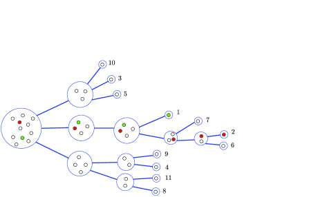
Figure 2: A sample tree $T_{[n]}$ for $n=11$, with the labeled leaves. The process $\Pi^{(11)}$ can be easily deduced: for instance, $\Pi^{(11)}(1)=\{\{1,2,6,7\},\{3,5,10\},\{4,8,9,11\}\}$. As opposed to Figure 1, leaves are all connected to vertices with at least $2$ children, because of the requirement $q_{1}(\varnothing)=1$.

distribution as $T_{\pi_{i}},1\leq i\leq b$, respectively. Since the law of the nonincreasing rearrangement of $\#\pi_{i},1\leq i\leq b$, is $q_{\#C}$, we readily obtain the following statement.

Lemma 24.

The tree $T_{C}$ has law $\mathsf{P}^{q}_{\#C}$.

In fact, the leaves of the tree $T_{C}$ are naturally labeled by elements of $C$. We will use this in the sequel, without further formalizing the notion of trees with labeled leaves.

We will also use the shorthand notation $T_{C}^{B}$ for the reduced tree $\theta(\Pi^{C}(\cdot),B)$. Using the above description, and applying the Markov property for $\Pi^{C}$ at time $D^{\Pi^{C}}_{B}$ and the particular form of the Markov kernel $Q$, we immediately obtain the following, in the particular case $B=[k],C=[n]$.

Proposition 25.

Let $2\leq k\leq n$. Then, conditionally on $D^{\Pi^{[n]}}_{[k]}=\ell$ and $\Pi^{[n]}(D^{\Pi^{[n]}}_{[k]})=\pi$, with $\pi|_{[k]}=\pi^{\prime}$, it holds that $T_{[n]}^{[k]}$ has same distribution as

$$\bigl{\langle}\theta^{(i)},1\leq i\leq b(\pi^{\prime})\bigr{\rangle}_{\ell},$$

where $\theta^{(i)},1\leq i\leq b$, are independent with respective laws that of $T_{\pi_{i}}^{\pi^{\prime}_{i}},1\leq i\leq b(\pi^{\prime})$.

The only subtle point is that $[k]\cap\pi_{i}=\pi^{\prime}_{i},1\leq i\leq b$, since the labeling of the blocks of $\pi,\pi^{\prime}$ could differ. But since these partitions are, respectively, of $[n]$ and $[k]$, this cannot be the case.

4 Proofs of Theorems 5 and 6

Let $q=(q_{n},n\geq 1)$ be a sequence of laws on $\mathcal{P}_{n}$, respectively, that satisfies (1) and (H), for some fragmentation pair $(-\gamma,\nu)$ and some slowly varying function $\ell$. In order to lighten notation, we let $a_{n}=n^{\gamma}\ell(n)$.

Consider a sequence of trees $(T_{n},n\geq 1)$, where $T_{n}$ has distribution $\mathsf{P}_{n}^{q}$, $n\geq 1$. As we noticed in the Introduction, it is easy to pass from the situation where $q_{1}(\varnothing)=1$ to the general situation, by adding independent linear strings with geometric$(q_{1}(\varnothing))$-distributed lengths to the $n$ leaves of $T_{n}$. Since geometric distributions have exponential tails, the longest of these $n$ strings will have a length at most $C\log n$ with probability going to $1$ as $n\to\infty$, for some $C>0$. If we let $T_{n}^{1}$ be the tree for which $q_{1}(\varnothing)>0$ and $T_{n}^{2}$ the one for which $q_{1}(\varnothing)=1$, coupled in the way depicted above, we easily get, for any $\gamma>0$,

$$\mathbb{P}\bigl{(}d_{\mathrm{GHP}}(a_{n}^{-1}T_{n}^{1},a_{n}^{-1}T_{n}^{2})\leq Ca_{n}^{-1}\log n\bigr{)}\mathop{\longrightarrow}_{n\to\infty}1.$$

Thus, we can deduce the convergence in distribution of $a_{n}^{-1}T_{n}^{1}$ to $\mathcal{T}_{\gamma,\nu}$ from that of $a_{n}^{-1}T_{n}^{2}$. Therefore, from now on and until the end of the present section, we make the following hypothesis, which will allow us to apply Lemma 24: [(H^′)]

The sequence $(q_{n},n\geq 1)$ satisfies (H) and $q_{1}(\varnothing)=1$.

4.1 Preliminary convergence lemmas

We now establish a couple of intermediate convergence results for the discrete model. Recall that the sequence of distributions $q_{n},n\geq 2$, on $\mathcal{P}_{n}$, respectively, induce distributions $p_{B}$ on $\mathcal{P}_{B}$ for finite $B$ by formula (13). By convention we set $p_{n}=p_{[n]}$.

Lemma 26.

Let $k\geq 2$, and let $\pi^{\prime}$ be an element in $\mathcal{P}_{[k]}$ with $b$ blocks, $b\geq 2$. Let $g\dvtx(0,\infty)^{b}\to\mathbb{R}$ be a continuous function with compact support. Then, under assumption (H^′),

$$a_{n}p_{n}\biggl{(}g\biggl{(}\frac{\#\pi_{1}}{n},\ldots,\frac{\#\pi_{b}}{n}\biggr{)}\mathbf{1}_{\{\pi|_{[k]}=\pi^{\prime}\}}\biggr{)}\mathop{\longrightarrow}_{n\to\infty}\int_{\mathcal{P}_{\mathbb{N}}}\kappa_{\nu}(\mathrm{d}\pi)g(|\pi_{1}|,\ldots,|\pi_{b}|)\mathbf{1}_{\{\pi|_{[k]}=\pi^{\prime}\}},$$

where $\kappa_{\nu}$ is the paintbox construction associated with $\nu$. Note that on the event $\{\pi|_{[k]}=\pi^{\prime}\}$, the quantities $\#\pi_{i}/n$ and $|\pi_{i}|$ for $1\leq i\leq b$ that appear above are a.e. nonzero, respectively, under $p_{n}$ and $\kappa_{\nu}$.

For simplicity, we let

$$B_{n}=p_{n}\biggl{(}g\biggl{(}\frac{\#\pi_{1}}{n},\ldots,\frac{\#\pi_{b}}{n}\biggr{)}\mathbf{1}_{\{\pi|_{[k]}=\pi^{\prime}\}}\biggr{)}.$$

Let $\lambda\in\mathcal{P}_{n}$, and let $i_{1},\ldots,i_{b}\in\mathbb{N}$ be pairwise distinct. This induces a sequence $(\lambda_{i_{1}},\ldots,\lambda_{i_{b}})$. Note that there are exactly

$$\prod_{l\geq 1}\frac{m_{l}(\lambda)!}{m_{l}(\lambda_{i},i\notin\{i_{1},\ldots,i_{b}\})!}$$

choices of such pairwise distinct indices $i^{\prime}_{1},\ldots,i^{\prime}_{b}$ such that $(\lambda_{i^{\prime}_{1}},\ldots,\lambda_{i^{\prime}_{b}})=(\lambda_{i_{1}},\ldots,\lambda_{i_{b}})$. Hence, by the definition of $q_{n}$ and Lemma 23,

$$B_{n} = \sum_{\lambda\in\mathcal{P}_{n}}q_{n}(\lambda)\mathop{\sum_{i_{1},\ldots,i_{b}\geq 1}}_{\mathrm{pairwise}\ \mathrm{distinct}}\prod_{l\geq 1}\frac{m_{l}(\lambda_{i},i\notin\{i_{1},\ldots,i_{b}\})!}{m_{l}(\lambda)!}g\biggl{(}\frac{\lambda_{i_{1}}}{n},\ldots,\frac{\lambda_{i_{b}}}{n}\biggr{)}$$

$$\hskip 117.8pt{}\times\frac{C_{\lambda}^{\pi^{\prime}}(i_{1},\ldots,i_{b})}{C_{\lambda}}$$

$$= \sum_{\lambda\in\mathcal{P}_{n}}q_{n}(\lambda)\frac{1}{(n)_{k}}\mathop{\sum_{i_{1},\ldots,i_{b}\geq 1}}_{\mathrm{pairwise}\ \mathrm{distinct}}g\biggl{(}\frac{\lambda_{i_{1}}}{n},\ldots,\frac{\lambda_{i_{b}}}{n}\biggr{)}\prod_{j=1}^{b}(\lambda_{i_{j}})_{\#\pi^{\prime}_{j}}.$$

Now, the function

$$h(\mathbf{s})=\mathop{\sum_{i_{1},\ldots,i_{b}\geq 1}}_{\mathrm{pairwise}\ \mathrm{distinct}}g(s_{i_{1}},\ldots,s_{i_{b}})\prod_{j=1}^{b}s_{i_{j}}^{\#\pi^{\prime}_{j}},\qquad\mathbf{s}\in{\mathcal{S}^{\downarrow}},$$

is continuous and bounded, because $g$ is compactly supported in $(0,\infty)^{b}$, so that the sum is really a finite sum. Moreover,

$$\qquad h(\mathbf{s})\leq K\mathop{\sum_{0\leq k_{1},k_{2},\ldots<k}}_{k_{1}+k_{2}+\cdots=k}\frac{k!}{\prod_{j\geq 1}k_{j}!}\prod_{j\geq 1}s_{j}^{k_{j}}=K\biggl{(}1-\sum_{j\geq 1}s_{j}^{k}\biggr{)}\leq kK(1-s_{1}),$$ (14)

where $K$ is an upper-bound of $|g|$, and for every $\lambda\in\mathcal{P}_{n}$, it is easily checked that for large $n$, if $\varepsilon>0$ is such that $g(x_{1},\ldots,x_{b})=0$ as soon as $\min_{1\leq i\leq b}x_{i}\leq\varepsilon$,

$$\biggl{(}1-\frac{k}{\varepsilon n}\biggr{)}^{k}h(\lambda/n) \leq \frac{1}{(n)_{k}}\mathop{\sum_{i_{1},\ldots,i_{b}\geq 1}}_{\mathrm{pairwise}\ \mathrm{distinct}}g\biggl{(}\frac{\lambda_{i_{1}}}{n},\ldots,\frac{\lambda_{i_{b}}}{n}\biggr{)}\prod_{j=1}^{b}(\lambda_{i_{j}})_{\#\pi^{\prime}_{j}}$$

$$\leq \biggl{(}\frac{n}{n-k}\biggr{)}^{k}h(\lambda/n).$$

Letting $n\to\infty$ and applying (H^′), which is validated by (14),

$$\lim_{n\to\infty}a_{n}B_{n}=\int_{\mathcal{S}^{\downarrow}}\nu(\mathrm{d}\mathbf{s})h(\mathbf{s})=\int_{\mathcal{P}_{\mathbb{N}}}\kappa_{\nu}(\mathrm{d}\pi)g(|\pi_{1}|,\ldots,|\pi_{b}|)\mathbf{1}_{\{\pi|_{[k]}=\pi^{\prime}\}},$$

the latter equality being a simple consequence of the paintbox construction of Section 3.1.2.

Now, we associate with $(q_{n},n\geq 1)$ a family of process $(\Pi^{B}(r),r\geq 0)$ with values in $\mathcal{P}_{B}$, as in Section 3.2.4. We let $\Pi^{n}=\Pi^{[n]}$ for simplicity, and set

$$D_{k}^{n}=D_{[k]}^{\Pi^{n}}=\inf\bigl{\{}r\geq 0\dvtx[k]\cap\Pi^{n}(r)\neq\{[k]\}\bigr{\}}$$

for $2\leq k\leq n$, and $D_{1}^{n}=D^{\Pi^{n}}_{\{1\}}=\inf\{r\geq 0\dvtx\{1\}\in\Pi^{n}(r)\}$. Also, for $r\geq 0$ we let

$$X_{n}(r)=\#\Pi^{n}_{(1)}(r).$$

Lemma 27.

Let $n,k\in\mathbb{N}$ be fixed, with $n\geq k\geq 2$, and let $\pi^{\prime}\in\mathcal{P}_{[k]}$ have $b\geq 2$ blocks. Let $F,f$ be measurable nonnegative functions. Then

$$\mathbb{E}\bigl{[}F\bigl{(}X_{n}\bigl{(}\cdot\wedge(D_{k}^{n}-1)\bigr{)}\bigr{)}f\bigl{(}\#\Pi^{n}_{i}(D_{k}^{n}),1\leq i\leq b\bigr{)}\mathbf{1}_{\{[k]\cap\Pi^{n}(D_{k}^{n})=\pi^{\prime}\}}\bigr{]}$$

$$\qquad=\sum_{r^{\prime}>0}\mathbb{E}\biggl{[}\frac{(X_{n}(r^{\prime}-1)-1)_{k-1}}{(n-1)_{k-1}}$$

$$\qquad\hphantom{=\sum_{r^{\prime}>0}\mathbb{E}\biggl{[}}{}\times F\bigl{(}X_{n}\bigl{(}\cdot\wedge(r^{\prime}-1)\bigr{)}\bigr{)}p_{X_{n}(r^{\prime}-1)}\bigl{(}f(\#\pi_{i},1\leq i\leq b)\mathbf{1}_{\{\pi|_{[k]}=\pi^{\prime}\}}\bigr{)}\biggr{]}.$$

We first consider an expression of a more general form. For nonnegative functions $G,g$, we have, using the Markov property at time $r^{\prime}-1$ in the second step,

$$\mathbb{E}\bigl{[}G\bigl{(}\Pi^{n}\bigl{(}\cdot\wedge(D_{k}^{n}-1)\bigr{)}\bigr{)}g\bigl{(}\Pi^{n}_{(1)}(D_{k}^{n}-1)\cap\Pi^{n}(D_{k}^{n})\bigr{)}\bigr{]}$$

$$\qquad=\sum_{r^{\prime}>0}\mathbb{E}\bigl{[}G\bigl{(}\Pi^{n}\bigl{(}\cdot\wedge(r^{\prime}-1)\bigr{)}\bigr{)}$$

$$\qquad\hphantom{=\sum_{r^{\prime}>0}\mathbb{E}\bigl{[}}{}\times\mathbf{1}_{\{[k]\subset\Pi^{n}_{(1)}(r^{\prime}-1)\}}g\bigl{(}\Pi^{n}_{(1)}(r^{\prime}-1)\cap\Pi^{n}(r^{\prime})\bigr{)}\mathbf{1}_{\{[k]\cap\Pi^{n}(r^{\prime})\neq\{[k]\}\}}\bigr{]}$$

$$\qquad=\sum_{r^{\prime}>0}\mathbb{E}\bigl{[}G\bigl{(}\Pi^{n}\bigl{(}\cdot\wedge(r^{\prime}-1)\bigr{)}\bigr{)}\mathbf{1}_{\{[k]\subset\Pi^{n}_{(1)}(r^{\prime}-1)\}}p_{\Pi^{n}_{(1)}(r^{\prime}-1)}\bigl{(}g(\pi)\mathbf{1}_{\{[k]\cap\pi\neq\{[k]\}\}}\bigr{)}\bigr{]}.$$

Specializing this formula to $G$ depending only on $X_{n}$ and $g(\pi)=f(\#\pi_{1},\ldots,\break\#\pi_{b})\mathbf{1}_{\{\pi|_{[k]}=\pi^{\prime}\}}$, and using obvious exchangeability properties, we obtain

$$\mathbb{E}\bigl{[}F\bigl{(}X_{n}\bigl{(}\cdot\wedge(D_{k}^{n}-1)\bigr{)}\bigr{)}f\bigl{(}\#\Pi^{n}_{i}(D_{k}^{n}),1\leq i\leq b\bigr{)}\mathbf{1}_{\{[k]\cap\Pi^{n}(D_{k}^{n})=\pi^{\prime}\}}\bigr{]}$$

$$\qquad=\sum_{r^{\prime}>0}\mathbb{E}\bigl{[}F\bigl{(}X_{n}\bigl{(}\cdot\wedge(r^{\prime}-1)\bigr{)}\bigr{)}$$

$$\qquad\hphantom{=\sum_{r^{\prime}>0}\mathbb{E}\bigl{[}}{}\times p_{X_{n}(r^{\prime}-1)}\bigl{(}f(\#\pi_{i},1\leq i\leq b)\mathbf{1}_{\{\pi|_{[k]}=\pi^{\prime}\}}\bigr{)}\mathbf{1}_{\{[k]\subset\Pi^{n}_{(1)}(r^{\prime}-1)\}}\bigr{]}.$$

All the terms in the expectation depend on $(X_{n}(r),0\leq r\leq r^{\prime}-1)$, except the last one which is a function of $\Pi^{n}_{(1)}(r^{\prime}-1)$. But by Lemma 13 (in fact, the variant used in the proof of Lemma 15),

$$\mathbb{P}\bigl{(}[k]\subset\Pi^{n}_{(1)}(r^{\prime}-1)|\bigl{(}X_{n}(r),0\leq r\leq r^{\prime}-1\bigr{)}\bigr{)}=\frac{(X_{n}(r^{\prime}-1)-1)_{k-1}}{(n-1)_{k-1}}$$

giving the result.

In the sequel, $\Pi(\cdot)$ will denote a continuous-time self-similar fragmentation with characteristic pair $(-\gamma,\nu)$, and $D_{k},k\geq 1$, will be defined as in Section 3.1.5.

Lemma 28.

Under assumption (H^′), it holds that

$$\biggl{(}\frac{X_{n}(\lfloor a_{n}t\rfloor)}{n},t\geq 0\biggr{)}\mathop{\longrightarrow}^{(d)}_{n\to\infty}\bigl{(}\bigl{|}\Pi_{(1)}(t)\bigr{|},t\geq 0\bigr{)},$$

in distribution for the Skorokhod topology, jointly with the convergence

$$\frac{1}{a_{n}}D^{n}_{1}\mathop{\longrightarrow}^{(d)}_{n\to\infty}D_{1}.$$

For $n>k\geq 1$, let $p_{n,k}=\mathbb{P}(X_{n}(1)=k)$. Note that the process $X_{n}$ is a nonincreasing Markov chain started from $n$, with probability transitions $p_{i,j},1\leq j\leq i$. Then by a simple exchangeability argument,

$$p_{n,k}=\sum_{\pi\in\mathcal{P}_{[n]}}p_{n}(\pi)m_{k}(\pi)\frac{k}{n}=\sum_{\lambda\in\mathcal{P}_{n}}q_{n}(\lambda)m_{k}(\lambda)\frac{k}{n},\qquad 1\leq k\leq n,$$

where $m_{k}(\pi)=m_{k}(\lambda(\pi))$ is the number of blocks of $\pi$ with size $k$. Consider the associated generating function for $x\geq 0$,

$$F_{n}(x) = \sum_{k=1}^{n}\biggl{(}\frac{k}{n}\biggr{)}^{x}p_{n,k}=\sum_{\lambda\in\mathcal{P}_{n}}q_{n}(\lambda)\sum_{k=1}^{n}m_{k}(\lambda)\biggl{(}\frac{k}{n}\biggr{)}^{x+1}$$

$$= \sum_{\lambda\in\mathcal{P}_{n}}q_{n}(\lambda)\sum_{i\geq 1}\biggl{(}\frac{\lambda_{i}}{n}\biggr{)}^{x+1}.$$

Hence, $1-F_{n}(x)=\overline{q}_{n}(f)$, where $f(\mathbf{s})=1-\sum_{i\geq 1}s_{i}^{x+1}$. Note that $f\dvtx{\mathcal{S}^{\downarrow}}\to\mathbb{R}$ is continuous whenever $x>0$. Indeed, the norm $\|\mathbf{s}\|_{x+1}=(\sum_{i\geq 1}s_{i}^{x+1})^{1/(x+1)}$ of any $\mathbf{s}\in{\mathcal{S}^{\downarrow}}$ is finite, and satisfies for every $\mathbf{s},\mathbf{s}^{\prime}\in{\mathcal{S}^{\downarrow}}$,

$$\bigl{|}\|\mathbf{s}\|_{x+1}-\|\mathbf{s}^{\prime}\|_{x+1}\bigr{|} \leq \|\mathbf{s}-\mathbf{s}^{\prime}\|_{x+1}$$

$$\leq \sup_{i\geq 1}|s_{i}-s^{\prime}_{i}|^{x/(1+x)}\biggl{(}\sum_{i\geq 1}s_{i}+\sum_{i\geq 1}s^{\prime}_{i}\biggr{)}^{1/(x+1)}$$

$$\leq 2^{1/(x+1)}d(\mathbf{s},\mathbf{s}^{\prime})^{x/(x+1)}.$$

Thus we may apply (H^′), and obtain

$$a_{n}\bigl{(}1-F_{n}(x)\bigr{)}\mathop{\longrightarrow}_{n\to\infty}\int_{\mathcal{S}^{\downarrow}}\biggl{(}1-\sum_{i\geq 1}s_{i}^{x+1}\biggr{)}\nu(\mathrm{d}\mathbf{s}).$$

This is exactly what we need to use HaMi09 , Theorem 1, stating that$(n^{-1}X_{n}(\lfloor a_{n}t\rfloor)$, $t\geq 0)$ converges in distribution to the self-similar Markov process $\exp(-\xi_{\tau(\cdot)})$, as defined around Proposition 19. Moreover, this convergence holds jointly with the convergence of absorption times at $1$, so $a_{n}^{-1}D_{1}^{n}$ converges to the absorption time at $0$ of $\exp(-\xi_{\tau(\cdot)})$. By Proposition 19, the process $\exp(-\xi_{\tau(\cdot)})$ has same distribution as $(|\Pi_{(1)}(t)|,t\geq 0)$, which reaches $0$ for the first time at time $D_{1}$. Hence the result.

Finally, the combination of the last two lemmas gives the last of our preliminary ingredients.

Lemma 29.

The following joint convergence in distribution holds:

$$\biggl{(}\frac{D_{k}^{n}}{a_{n}},[k]\cap\Pi^{n}(D_{k}^{n}),\biggl{(}\frac{\#\Pi^{n}_{(i)}(D_{k}^{n})}{n},i\in[k]\biggr{)}\biggr{)}$$

$$\qquad\mathop{\longrightarrow}^{(d)}_{n\to\infty}\bigl{(}D_{k},[k]\cap\Pi(D_{k}),\bigl{(}\bigl{|}\Pi_{(i)}(D_{k})\bigr{|},i\in[k]\bigr{)}\bigr{)}.$$

Let $\pi^{\prime}\in\mathcal{P}_{k}$ have $b\geq 2$ blocks, and $f,g\dvtx(0,\infty)\to\mathbb{R},h\dvtx(0,\infty)^{b}\to\mathbb{R}$ be continuous functions with compact support. Then by Lemma 27,

$$\mathbb{E}\biggl{[}f\biggl{(}\frac{D_{k}^{n}}{a_{n}}\biggr{)}g\biggl{(}\frac{X_{n}(D_{k}^{n}-1)}{n}\biggr{)}h\biggl{(}\frac{\#\Pi^{n}_{i}(D_{k}^{n})}{X_{n}(D_{k}^{n}-1)},1\leq i\leq b\biggr{)}\mathbf{1}_{\{[k]\cap\Pi^{n}(D_{k}^{n})=\pi^{\prime}\}}\biggr{]}$$

$$\qquad=\sum_{r^{\prime}>0}f\biggl{(}\frac{r^{\prime}}{a_{n}}\biggr{)}\mathbb{E}\biggl{[}\frac{(X_{n}(r^{\prime}-1)-1)_{k-1}}{(n-1)_{k-1}}g\biggl{(}\frac{X_{n}(r^{\prime}-1)}{n}\biggr{)}$$

$$\qquad\hphantom{=\sum_{r^{\prime}>0}f\biggl{(}\frac{r^{\prime}}{a_{n}}\biggr{)}\mathbb{E}\biggl{[}}{}\times p_{X_{n}(r^{\prime}-1)}\biggl{(}h\biggl{(}\frac{\#\pi_{i}}{X_{n}(r^{\prime}-1)},1\leq i\leq b\biggr{)}\mathbf{1}_{\{\pi|_{[k]}=\pi^{\prime}\}}\biggr{)}\biggr{]}$$

$$\qquad=\frac{1}{a_{n}}\sum_{r^{\prime}>0}f\biggl{(}\frac{r^{\prime}}{a_{n}}\biggr{)}\mathbb{E}\biggl{[}\Phi\bigl{(}n,X_{n}(r^{\prime}-1)\bigr{)}g\biggl{(}\frac{X_{n}(r^{\prime}-1)}{n}\biggr{)}\Psi\bigl{(}X_{n}(r^{\prime}-1)\bigr{)}\biggr{]}$$

$$\qquad=\int_{1/a_{n}}^{\infty}f\biggl{(}\frac{\lfloor a_{n}u\rfloor}{a_{n}}\biggr{)}\,\mathrm{d}u\mathbb{E}\biggl{[}\Phi\bigl{(}n,X_{n}(\lfloor a_{n}u\rfloor-1)\bigr{)}$$

$$\qquad\hphantom{=\int_{1/a_{n}}^{\infty}f\biggl{(}\frac{\lfloor a_{n}u\rfloor}{a_{n}}\biggr{)}\,\mathrm{d}u\mathbb{E}\biggl{[}}\times g\biggl{(}\frac{X_{n}(\lfloor a_{n}u\rfloor-1)}{n}\biggr{)}\Psi\bigl{(}X_{n}(\lfloor a_{n}u\rfloor-1)\bigr{)}\biggr{]},$$

where

$$\Phi(n,x)=\frac{(x-1)_{k-1}}{(n-1)_{k-1}}\frac{a_{n}}{a_{x}}\mathop{\longrightarrow}_{(n,x/n)\to(\infty,c)}c^{k-1-\gamma}$$

and

$$\Psi(m)=a_{m}p_{m}\biggl{(}h\biggl{(}\frac{\#\pi_{i}}{m},1\leq i\leq b\biggr{)}\mathbf{1}_{\{\pi|_{[k]}=\pi^{\prime}\}}\biggr{)}.$$

Note that the Potter’s bounds for regularly varying functions (BGT , Theorem 1.5.6) imply that $\Phi(n,x)\leq C(\frac{x}{n})^{k-1-\gamma-1}$ for all $n\geq x\geq A$ for some finite positive constants $C,A$. In particular there exists some $n_{0}$ such that $\sup_{n\geq n_{0},0<x\leq n}\Phi(n,x)\times g(x/n)<\infty$ (since $g$ is null in a neighborhood of 0). The joint use of Lemmas 26 and 28 entails by dominated convergence that the expectation term in the integral converges to (note that the quantities $|\pi_{i}|,1\leq i\leq b$, are all a.e. positive on $\{\pi|_{[k]}=\pi^{\prime}\}$ under $\kappa_{\nu}$)

$$\mathbb{E}\biggl{[}\bigl{|}\Pi_{(1)}(u)\bigr{|}^{k-1-\gamma}g\bigl{(}\bigl{|}\Pi_{(1)}(u)\bigr{|}\bigr{)}\int_{\mathcal{P}_{\mathbb{N}}}\kappa_{\nu}(\mathrm{d}\pi)h(|\pi_{i}|,1\leq i\leq b)\mathbf{1}_{\{\pi|_{[k]}=\pi^{\prime}\}}\biggr{]},$$

and since $f,g,h$ are compactly supported, the whole integral converges to

$$\int_{0}^{\infty}f(u)\,\mathrm{d}u\mathbb{E}\biggl{[}\bigl{|}\Pi_{(1)}(u)\bigr{|}^{k-1-\gamma}g\bigl{(}\bigl{|}\Pi_{(1)}(u)\bigr{|}\bigr{)}$$

$$\qquad\hskip 44.8pt{}\times\int_{\mathcal{P}_{\mathbb{N}}}\kappa_{\nu}(\mathrm{d}\pi)h(|\pi_{i}|,1\leq i\leq b)\mathbf{1}_{\{\pi|_{[k]}=\pi^{\prime}\}}\biggr{]},$$

which, by Proposition 18, equals

$$\mathbb{E}\biggl{[}f(D_{k})g\bigl{(}\bigl{|}\Pi_{(1)}(D_{k}-)\bigr{|}\bigr{)}h\biggl{(}\frac{|\Pi_{i}(D_{k})|}{|\Pi_{(1)}(D_{k}-)|},1\leq i\leq b\biggr{)}\mathbf{1}_{\{[k]\cap\Pi(D_{k})=\pi^{\prime}\}}\biggr{]}.$$

It is now easy to conclude, since $|\Pi_{i}(D_{k})|>0$ almost-surely.

4.2 Convergence of finite-dimensional marginals

The first step in the proof of Theorem 5 is the following result on reduced trees $T_{C}^{B}$ of Section 3.2.4.

Proposition 30.

Let $B\subset\mathbb{N}$ be finite. Under assumption (H^′), we have the following convergence in distribution in $\mathscr{T}_{\mathrm{w}}$:

$$\frac{1}{a_{n}}T_{[n]}^{B}\mathop{\longrightarrow}^{(d)}_{n\to\infty}\mathcal{R}(\mathcal{T}_{\gamma,\nu},B).$$

We use an induction argument on the cardinality of $B$. For $B=\{i\}$, one can assume by exchangeability (as soon as $n\geq i$) that $B=\{1\}$, and in this case, the reduced tree is $T_{[n]}^{B}=(\varnothing,D_{1}^{n})$, while $\mathcal{R}(\mathcal{T}_{\gamma,\nu},\{1\})=(\varnothing,D_{1})$ by Proposition 22. By the second part of Lemma 28, under (H^′), it holds that

$$\frac{D^{n}_{1}}{a_{n}}\mathop{\longrightarrow}^{(\mathrm{d})}_{n\to\infty}D_{1}.$$

This initializes the induction. Now, assume that Proposition 30 has been proved for every set $B$ with cardinality at most $k-1$, for some $k\geq 2$. We want to show that the same is true of any set of cardinality $k$, and by exchangeability, we may assume that $B=[k]$.

We now recall, using Proposition 25, that conditionally on $D_{k}^{n}=\ell$, $[k]\cap\Pi^{n}(D_{k}^{n})=\pi^{\prime}$ having $b\geq 2$ blocks and on $\Pi^{n}_{i}(D_{k}^{n})=\pi_{i},1\leq i\leq b$, with respective cardinality $\#\pi_{i}=n_{i}$, the tree $T_{[n]}^{[k]}$ has same distribution as

$$\bigl{\langle}\theta^{(i)},1\leq i\leq b\bigr{\rangle}_{\ell},$$

where $\theta^{(i)}$ has same distribution as $T^{\pi^{\prime}_{i}}_{\pi_{i}}$, and these trees are independent.

The joint distribution of $D_{k}^{n},[k]\cap\Pi^{n}(D_{k}^{n}),(\#\Pi^{n}_{(i)}(D_{k}^{n}),1\leq i\leq k)$ is specified by Lemma 27, and its scaling limit by Lemma 29. We obtain by the induction hypothesis that jointly with the above convergence, conditionally on $[k]\cap\Pi^{n}(D_{k}^{n})=\pi^{\prime}$,

$$\frac{1}{a_{n}}\theta^{(i)} = \frac{a_{n_{i}}}{a_{n}}\frac{1}{a_{n_{i}}}\theta^{(i)}$$

$$\displaystyle\mathop{\longrightarrow}^{(\mathrm{d})}_{n\to\infty} |\Pi_{i}(D_{k})|^{\gamma}\mathcal{T}^{(i)},\qquad 1\leq i\leq b,$$

where the $\mathcal{T}^{(i)}$ are independent with same laws as $\mathcal{R}(\mathcal{T}_{\gamma,\nu},\pi^{\prime}_{i})$, respectively. Finally, $a_{n}^{-1}T^{[k]}_{[n]}$ converges to

$$\bigl{\langle}|\Pi_{i}(D_{k})|^{\gamma}\mathcal{T}^{(i)},1\leq i\leq b\bigr{\rangle}_{D_{k}},$$

and the $\mathbb{R}$-tree associated with this tree has same distribution as $\mathcal{R}(\mathcal{T}_{\gamma,\nu},[k])$ by Proposition 22.

4.3 Tightness in the Gromov–Hausdorff topology

We now want to improve the convergence of Proposition 30 into a convergence of nonreduced trees for the Gromov–Hausdorff topology. Namely

Proposition 31.

Under hypothesis (H^′), we have the convergence in distribution

$$\frac{1}{a_{n}}T_{n}\mathop{\longrightarrow}^{(d)}_{n\to\infty}\mathcal{T}_{\gamma,\nu}$$

in $\mathscr{T}$, for the Gromov–Hausdorff topology.

This will be proved by first showing a couple of intermediate lemmas.

Lemma 32.

Under assumption (H^′), we have the convergence in distribution

$$\bigl{(}\Pi^{n}(\lfloor a_{n}t\rfloor),t\geq 0\bigr{)}\mathop{\longrightarrow}^{(d)}_{n\to\infty}\bigl{(}\Pi(t),t\geq 0\bigr{)}$$

jointly with

$$\biggl{(}\frac{\#\Pi^{n}_{(i)}(\lfloor a_{n}t\rfloor)}{n},t\geq 0\biggr{)}\mathop{\longrightarrow}^{(d)}_{n\to\infty}\bigl{(}\bigl{|}\Pi_{(i)}(t)\bigr{|},t\geq 0\bigr{)}$$

for every $i\geq 1$, all these convergences holding jointly.

The fact that $([k]\cap\Pi^{n}(\lfloor a_{n}t\rfloor),t\geq 0)$ converges in the Skorokhod space to $([k]\cap\Pi(t),t\geq 0)$ for every $k\geq 1$ is obtained by using an inductive argument similar to that used in the proof of Proposition 30. We only sketch the argument. The statement is trivial for $k=1$, so we can assume that $k\geq 2$. The process $[k]\cap\Pi^{n}(\lfloor a_{n}\cdot\rfloor)$ remains constant equal to $[k]$ up to time $a_{n}^{-1}D^{n}_{k}$, and jumps to the state $\pi^{\prime}=[k]\cap\pi$, $\pi=\Pi^{n}(D^{n}_{k})$. By Lemma 29, $a_{n}^{-1}D^{n}_{k}\to D_{k}$ as $n\to\infty$, and the latter has a diffuse law by Proposition 18.

After time $a_{n}^{-1}D^{n}_{k}$, given $\pi$, the restrictions $\pi^{\prime}_{i}\cap\Pi^{n}(\lfloor a_{n}\cdot\rfloor+D^{n}_{k})$ have same distribution as $\pi^{\prime}_{i}\cap\Pi^{\pi_{i}}(\lfloor a_{n}\cdot\rfloor)$ and are independent. By the induction hypothesis and exchangeability, still conditionally on $\pi$, this converges to $\pi^{\prime}_{i}\cap\Pi^{(i)}(\cdot)$, where $\Pi^{(i)},i\geq 1$, are i.i.d. copies of $\Pi$. Moreover, since the jump times have diffuse laws, two such copies never jump at the same time, from which one concludes that given $\pi$, the process $(\pi^{\prime}_{i}\cap\Pi^{n}(\lfloor a_{n}t\rfloor+D^{n}_{k}),1\leq i\leq b(\pi^{\prime}),t\geq 0)$ converges in the Skorokhod space to $(\pi^{\prime}_{i}\cap\Pi^{(i)}(t),1\leq i\leq b(\pi^{\prime}),t\geq 0)$. This concludes the inductive step by gluing on the initial constancy interval of the process, with length $a_{n}^{-1}D^{n}_{k}$.

The convergence of $\Pi^{n}(\lfloor a_{n}\cdot\rfloor)$ in the Skorokhod space follows, because $d_{\mathcal{P}}([k]\cap\pi,\pi)\leq e^{-k}$ for every $\pi\in\mathcal{P}_{\mathbb{N}}$. This shows that $[k]\cap\Pi^{n}(\lfloor a_{n}\cdot\rfloor)$ remains uniformly close to $\Pi^{n}(\lfloor a_{n}\cdot\rfloor)$.

Next, by Lemma 14, it follows that, jointly with this convergence, for every $i\geq 1$, the one-dimensional marginals of $(n^{-1}\#\Pi^{n}_{(i)}(\lfloor a_{n}t\rfloor),t\geq 0)$ converge in distribution to those of $(|\Pi_{(i)}(t)|,t\geq 0)$, at least for times which are not fixed discontinuity times of the limiting process—the set of such points is always countable, and it turns out that there are none in the present case. The convergence of finite-dimensional marginals (outside of possible fixed discontinuities) is obtained in a similar way, using a straightforward generalization of Lemma 14 to the case of a sequence $((\pi^{(n,1)},\ldots,\pi^{(n,k)}),n\geq 1)$ of jointly exchangeable random partitions, respectively, of $[n]$, that converges to a limiting $k$-tuple of random partitions of $\mathbb{N}$. This generalization is left to the reader.

Since we also know that the laws of the processes $(n^{-1}\#\Pi^{n}_{(i)}(\lfloor a_{n}t\rfloor),t\geq 0)$ are tight when $n$ varies, by Lemma 28 (these processes all have same distribution as $(n^{-1}X_{n}(\lfloor a_{n}t\rfloor),t\geq 0)$ by exchangeability), this allows us to conclude.

For $k+1\leq i\leq n$, let

$$S_{i}^{n}=\inf\bigl{\{}r\geq 0\dvtx[k]\cap\Pi^{n}_{(i)}(r)=\varnothing\bigr{\}},$$

the first time when the ball indexed $i$ is separated from the $k$ first balls. The random variables $S^{n}_{i},k+1\leq i\leq n$, have same distribution by exchangeability. The strong Markov property at the stopping time $S_{i}^{n}$ also shows that conditionally on $\Pi^{n}_{(i)}(S_{i}^{n})=B$, the process $(B\cap\Pi^{n}(S_{i}^{n}+r),r\geq 0)$ has same distribution as $\Pi^{B}$. Conditionally on $\Pi^{n}_{(i)}(S_{i}^{n})=B$, the tree $\mathsf{t}_{B\cap\Pi^{n}(S_{i}^{n}+\cdot)}$ has thus the same distribution as $T_{B}$ and can be seen as a subtree of $T_{[n]}$, characterized by the fact that this subtree contains the leaf labeled $i$, does not contain any of the leaves labeled by an element of $[k]$ and is the maximal subtree of $T_{[n]}$ with this property. In particular, the Gromov–Hausdorff distance between $T_{[n]}^{[k]}$ and $T_{[n]}$ is at most

$$d_{\mathrm{GH}}\bigl{(}T_{[n]}^{[k]},T_{[n]}\bigr{)}\leq\max_{k+1\leq i\leq n}\mathrm{ht}\bigl{(}\mathsf{t}_{\Pi^{n}_{(i)}(S^{n}_{i})\cap\Pi^{n}(S_{i}^{n}+\cdot)}\bigr{)},$$

where $\mathrm{ht}(\mathsf{t})$, called the height of $\mathsf{t}$, is the maximal height of a vertex in $\mathsf{t}$.

Note that if $j\in\Pi^{n}_{(i)}(S^{n}_{i})$, then $S^{n}_{j}=S^{n}_{i}$. Therefore, the blocks $\Pi^{n}_{(i)}(S^{n}_{i}),k+1\leq i\leq n$, are either disjoint or equal. Moreover, the partition $\pi$ of $[n]\setminus[k]$ with these blocks is clearly exchangeable. By putting the previous observations together, we obtain by first conditioning on $\pi$, and for every $\eta>0$,

$$\mathbb{P}\bigl{(}d_{\mathrm{GH}}\bigl{(}T_{[n]}^{[k]},T_{[n]}\bigr{)}\geq\eta a_{n}\bigr{)}\leq\mathbb{E}\biggl{[}\sum_{i\geq 1}\mathsf{P}^{q}_{\#\pi_{i}}(\mathrm{ht}\geq\eta a_{n})\biggr{]},\qquad\eta>0.$$ (15)

Here and later, we adopt the convention that quantities involving $\#\pi_{i}$ are always equal to $0$ when $\#\pi_{i}=0$. At this point, we need the following uniform estimate for the height of a $\mathsf{P}^{q}_{n}$-distributed tree, which is the key lemma of this section.

Lemma 33.

Assume (H^′). Then for all $p>0$, there exists a finite constant $C_{p}$ such that

$$\mathsf{P}_{n}^{q}(\mathrm{ht}\geq xa_{n})\leq\frac{C_{p}}{x^{p}}\qquad\forall x>0,\forall n\geq 1.$$

Before giving the proof of this statement, we end the proof of Proposition 31. Using Lemma 33 for $p=2/\gamma$ and (15), we obtain

$$\mathbb{P}\bigl{(}d_{\mathrm{GH}}\bigl{(}T_{[n]}^{[k]},T_{[n]}\bigr{)}\geq\eta a_{n}\bigr{)}\leq C_{2/\gamma}\eta^{-2/\gamma}\mathbb{E}\biggl{[}\sum_{i\geq 1}\frac{a_{\#\pi_{i}}^{2/\gamma}}{a_{n}^{2/\gamma}}\biggr{]}.$$

By the exchangeability of the partition $\pi$ of $[n]\setminus[k]$, note that for every measurable function $f$,

$$\mathbb{E}\bigl{[}f\bigl{(}\#\pi_{(k+1)}\bigr{)}\bigr{]}=\frac{1}{n-k}\mathbb{E}\Biggl{[}\sum_{i=k+1}^{n}f\bigl{(}\#\pi_{(i)}\bigr{)}\Biggr{]}=\mathbb{E}\biggl{[}\sum_{i\geq 1}\frac{\#\pi_{i}}{n-k}f(\#\pi_{i})\biggr{]}.$$

This finally yields

$$\mathbb{P}\bigl{(}d_{\mathrm{GH}}\bigl{(}T_{[n]}^{[k]},T_{[n]}\bigr{)}\geq\eta a_{n}\bigr{)}\leq C_{2/\gamma}\eta^{-2/\gamma}\mathbb{E}\biggl{[}\frac{a_{\#\pi_{(k+1)}}^{2/\gamma}(\#\pi_{(k+1)})^{-1}}{a_{n}^{2/\gamma}n^{-1}}\biggr{]}.$$

Since the sequence $(a_{n}^{2/\gamma}n^{-1},n\geq 1)$ is strictly positive and regularly varying at $\infty$ with index 1, we get from Potter’s bounds (BGT , Theorem 1.5.6), the existence of a finite constant $C$ such that $(a_{k}^{2/\gamma}k^{-1})/(a_{n}^{2/\gamma}n^{-1})\leq C\sqrt{k/n}$ for all $1\leq k\leq n$. Hence,

$$\mathbb{P}\bigl{(}d_{\mathrm{GH}}\bigl{(}T_{[n]}^{[k]},T_{[n]}\bigr{)}\geq\eta a_{n}\bigr{)}\leq CC_{2/\gamma}\eta^{-2/\gamma}\mathbb{E}\Biggl{[}\sqrt{\frac{\#\pi_{(k+1)}}{n}}\Biggr{]}.$$

Note that the quantity in the expectation is bounded by 1. By Lemma 32, it holds that $S^{n}_{k+1}/a_{n}\to S_{k+1}$ in distribution as $n\to\infty$, where $S_{k+1}=\inf\{t\geq 0\dvtx[k]\cap\Pi_{(k+1)}(t)=\varnothing\}$. This convergence holds jointly with that of $(n^{-1}\#\Pi^{n}_{(k+1)}(\lfloor a_{n}t\rfloor)$, $t\geq 0)$ to $(|\Pi_{(k+1)}(t)|,t\geq 0)$ in the Skorokhod space, whence we deduce that

$$\limsup_{n\to\infty}\mathbb{P}\bigl{(}d_{\mathrm{GH}}\bigl{(}T_{[n]}^{[k]},T_{[n]}\bigr{)}\geq\eta a_{n}\bigr{)}\leq CC_{2/\gamma}\eta^{-2/\gamma}\mathbb{E}\bigl{[}\sqrt{\bigl{|}\Pi_{(k+1)}(S_{k+1}-)}\bigr{|}\bigr{]}.$$

Let $S^{\prime}_{k+1}=\inf\{t\geq 0\dvtx\{2,3,\ldots,k+1\}\cap\Pi_{(1)}(t)=\varnothing\}$, then by exchangeability,

$$\limsup_{n\to\infty}\mathbb{P}\bigl{(}d_{\mathrm{GH}}\bigl{(}T_{[n]}^{[k]},T_{[n]}\bigr{)}\geq\eta a_{n}\bigr{)}\leq CC_{2/\gamma}\eta^{-2/\gamma}\mathbb{E}\bigl{[}\sqrt{\bigl{|}\Pi_{(1)}(S^{\prime}_{k+1}-)}\bigr{|}\bigr{]}.$$

Since the quantity in the expectation goes to $0$ a.s. as $k\to\infty$ and is bounded [indeed $S^{\prime}_{k}\uparrow D_{\{1\}}$ a.s. and $|\Pi_{(1)}(D_{\{1\}}-)|=0$ by (2) and Proposition 19], we conclude that for every $\eta>0$,

$$\lim_{k\to\infty}\limsup_{n\to\infty}\mathbb{P}\bigl{(}d_{\mathrm{GH}}\bigl{(}T_{[n]}^{[k]},T_{[n]}\bigr{)}\geq\eta a_{n}\bigr{)}=0.$$ (16)

It is now easy to get from this the convergence in distribution of $a_{n}^{-1}T_{[n]}$ toward $\mathcal{T}_{\gamma,\nu}$ in $(\mathscr{T},d_{\mathrm{GH}})$, using the following lemma, together with (16), Proposition 30 and the fact that $\mathcal{R}(\mathcal{T}_{\gamma,\nu},[k])$ converges in distribution in $(\mathscr{T},d_{\mathrm{GH}})$ to $\mathcal{T}_{\gamma,\nu}$ as $k\to\infty$ HM04 .

Lemma 34 ((billingsley99 , Theorem 3.2)).

Let $X_{n},X,X_{n}^{k},X^{k}$ be random variables in a metric space $(M,d)$. We assume that for every $k$, we have $X_{n}^{k}\to X^{k}$ in distribution as $n\to\infty$, and $X^{k}\to X$ in distribution as $k\to\infty$. Finally, we assume that for every $\eta>0$,

$$\lim_{k\to\infty}\limsup_{n\to\infty}\mathbb{P}\bigl{(}d(X_{n}^{k},X_{n})>\eta\bigr{)}=0.$$

Then $X_{n}\to X$ in distribution as $n\to\infty$.

Proof of Lemma 33 Note that if the statement holds for some $p>0$, it then holds for all $p^{\prime}\in(0,p)$. We can therefore assume in the following that $p>1/\gamma$, and we let $\varepsilon>0$ be so that $p(\gamma-\varepsilon)>1$. The main idea of the proof is to proceed by induction on $n$, using the Markov branching property. We start with some technical preliminaries.

$\bullet$ First note that $\mathsf{E}_{n}^{q}[\mathrm{ht}^{r}]<\infty$ for all $r>0$ and all $n\geq 1$. This can easily be proved by induction on $n$ ($r$ being fixed) using the Markov branching property and the facts that $q_{n}((n))<1$ and that $\mathrm{ht}=0$ almost-surely under $\mathsf{P}_{1}^{q}$.

$\bullet$ Second, we replace the sequence $(a_{n},n\geq 1)$ by a “nicer” sequence $(\tilde{a}_{n},n\geq 1)$ such that $\tilde{a}_{n}\sim a_{n}$, that is, $a_{n}/\tilde{a}_{n}\rightarrow 1$ as $n\rightarrow\infty$. This step is trivial when $a_{n}=n^{\gamma}$; we then take $\tilde{a}_{n}=a_{n}$. Since $a_{n}=n^{\gamma}\ell(n)$ with $\ell$ slowly varying at $\infty$, it is well known (see BGT , Theorem 1.3.1) that it can be written in the form

$$a_{n}=n^{\gamma}c(n)\exp\biggl{(}\int_{1}^{n}\eta(u)\,\mathrm{d}u/u\biggr{)},\qquad n\geq 1,$$

where $c(n)\rightarrow c>0$ as $n\rightarrow\infty$, and $\eta$ is a measurable function that converges to $0$ as $u\rightarrow\infty$. Define

$$\tilde{a}_{n}=n^{\gamma}c\exp\biggl{(}\int_{1}^{n}\eta(u)\,\mathrm{d}u/u\biggr{)},\qquad n\geq 1.$$

We claim that there exists an integer $n_{\varepsilon}\geq 1$ such that for $n\geq n_{\varepsilon}$,

$$\frac{\tilde{a}_{k}}{\tilde{a}_{n}}\leq\biggl{(}\frac{k}{n}\biggr{)}^{\gamma-\varepsilon}\qquad\forall 1\leq k\leq n.$$ (17)

Indeed, let $u_{\varepsilon}$ be such that $|\eta(u)|\leq\varepsilon$ for all $u\geq u_{\varepsilon}$. For $n\geq k\geq u_{\varepsilon}$, we have

$$\biggl{|}\int_{k}^{n}-\eta(u)\,\mathrm{d}u/u\biggr{|}\leq\varepsilon\int_{k}^{n}\mathrm{d}u/u\leq\varepsilon\ln(n/k);$$

hence

$$\frac{\tilde{a}_{k}}{\tilde{a}_{n}}=\biggl{(}\frac{k}{n}\biggr{)}^{\gamma}\exp\biggl{(}-\int_{k}^{n}\eta(u)\,\mathrm{d}u/u\biggr{)}\leq\biggl{(}\frac{k}{n}\biggr{)}^{\gamma-\varepsilon}.$$

Besides $\sup_{k\in\{1,\ldots,\lfloor u_{\varepsilon}\rfloor\}}\tilde{a}_{k}k^{\varepsilon-\gamma}/(\tilde{a}_{n}n^{\varepsilon-\gamma})\leq 1$ for all $n$ large enough (say $n\geq n^{\prime}_{\varepsilon}$). Hence $\tilde{a}_{k}/\tilde{a}_{n}\leq(k/n)^{\gamma-\varepsilon}$ for all $n\geq n_{\varepsilon}=\max(n^{\prime}_{\varepsilon},u_{\varepsilon})$ and all $1\leq k\leq n$.

$\bullet$ Since $a_{n}>0$ for all $n\geq 1$ and $\tilde{a}_{n}\sim a_{n}$, there exists some $C>0$ such that $a_{n}\geq C\tilde{a}_{n}$ for all $n\geq 1$. It is therefore sufficient to prove the existence of a finite $C_{p}$ (a priori different from the one in the statement of the lemma) such that

$$\mathsf{P}^{q}_{n}(\mathrm{ht}\geq x\tilde{a}_{n})\leq\frac{C_{p}}{x^{p}}\qquad\forall x>0\mbox{ and }n\geq 1,$$ (18)

to finish the proof of the lemma. In order to prove (18), we will use the integer $n_{\varepsilon}$ introduced around (17), and we will further assume, taking $n_{\varepsilon}$ larger if necessary, that $\tilde{a}_{n}\geq 1$ for every $n\geq n_{\varepsilon}$. Introduce now $0<C^{1}_{p}<1$ such that

$$(1-u)^{-p}\leq 1+2pu\qquad\forall 0\leq u\leq C^{1}_{p}.$$

Using (H^′) and the fact that $q_{n}((n))<1$ for all $n\geq 1$, there exists also $C^{2}_{p}>0$ such that

$$\tilde{a}_{n}\sum_{\lambda\in\mathcal{P}_{n}}q_{n}(\lambda)\Biggl{(}1-\sum_{i=1}^{p(\lambda)}\biggl{(}\frac{\lambda_{i}}{n}\biggr{)}^{(\gamma-\varepsilon)p}\Biggr{)}\geq C^{2}_{p}\qquad\forall n\geq 1$$ (19)

[recall that $(\gamma-\varepsilon)p>1$ and $\tilde{a}_{n}>0$ for all $n\geq 1$]. Last we let

$$C_{p}(n_{\varepsilon}):=\max_{1\leq n\leq n_{\varepsilon}}(\mathsf{E}_{n}^{q}[\mathrm{ht}^{p}]/\tilde{a}_{n}^{p})<\infty,$$

and we set

$$C_{p}:=\max\bigl{(}C_{p}(n_{\varepsilon}),(1/C^{1}_{p})^{p},(2p/C^{2}_{p})^{p}\bigr{)}<\infty.$$

Our goal is to prove by induction on $n\geq 1$ that

$$\hypertarget{AN}{\mathsf{P}}_{n}^{q}(\mathrm{ht}<x\tilde{a}_{n})\geq 1-\frac{C_{p}}{x^{p}}\qquad\mbox{for every }x>0. \mathrm{A}_{n}$$ ()

Clearly, ($\mathrm{A}_{n}$) holds for all $n\leq n_{\varepsilon}$ since $C_{p}\geq C_{p}(n_{\varepsilon})$ and $\mathsf{P}_{n}^{q}(\mathrm{ht}\geq x\tilde{a}_{n})\leq\mathsf{E}_{n}^{q}[\mathrm{ht}^{p}]/(x\tilde{a}_{n})^{p}$. Now assume that ($\mathrm{A}_{k}$) is satisfied for all $k\leq n-1$ for some $n\geq n_{\varepsilon}$. For all $0<x\leq C_{p}^{1/p}$, the expected inequalities in ($\mathrm{A}_{n}$) are obvious, so it remains to prove them for $x>C_{p}^{1/p}$. To get ($\mathrm{A}_{n}$), we will prove by induction on $i\in\mathbb{N}$ that

$$\hypertarget{ANI}{\mathsf{P}}_{n}^{q}(\mathrm{ht}<x\tilde{a}_{n})\geq 1-\frac{C_{p}}{x^{p}}\qquad\mbox{for every }x\in\biggl{(}0,\frac{i}{\tilde{a}_{n}}\biggr{)}, \mathrm{A}_{n,i}$$ ()

which will obviously lead to ($\mathrm{A}_{n}$). Note first that ($\mathrm{A}_{n,1}$) holds since $1/\tilde{a}_{n}\leq 1\leq C_{p}^{1/p}$. Assume next that ($\mathrm{A}_{n,i}$) is true, and fix $x\in(0,(i+1)/\tilde{a}_{n})$. We can assume that $x>C_{p}^{1/p}$ since ($\mathrm{A}_{n}$) holds otherwise. Using the Markov branching property and the fact that ($\mathrm{A}_{k}$) holds for every $k\leq n-1$, as well as ($\mathrm{A}_{n,i}$), we then get

$$\mathsf{P}_{n}^{q}(\mathrm{ht}<x\tilde{a}_{n}) = \sum_{\lambda\in\mathcal{P}_{n}}q_{n}(\lambda)\prod_{i=1}^{p(\lambda)}\mathsf{P}_{\lambda_{i}}^{q}(\mathrm{ht}<x\tilde{a}_{n}-1)$$

$$\geq \sum_{\lambda\in\mathcal{P}_{n}}q_{n}(\lambda)\prod_{i=1}^{p(\lambda)}\biggl{(}1-\frac{C_{p}\tilde{a}_{\lambda_{i}}^{p}}{(x\tilde{a}_{n}-1)^{p}}\biggr{)}^{+}$$

$$\geq \sum_{\lambda\in\mathcal{P}_{n}}q_{n}(\lambda)\Biggl{(}1-\sum_{i=1}^{p(\lambda)}\frac{C_{p}\tilde{a}_{\lambda_{i}}^{p}}{(x\tilde{a}_{n}-1)^{p}}\Biggr{)}$$

using the notation $r^{+}=\max(r,0)$ and that for all sequences of nonnegative terms $b_{i},i\geq 1$, $\prod_{i=1}^{m}(1-b_{i})^{+}\geq 1-\sum_{i=1}^{m}b_{i}$, for every $m\geq 1$. Next, since $x\tilde{a}_{n}\geq x>1/C_{p}^{1}>1$,

$$\frac{1}{(x\tilde{a}_{n}-1)^{p}}=\frac{1}{(x\tilde{a}_{n})^{p}(1-1/(x\tilde{a}_{n}))^{p}}\leq\frac{1+2p/(x\tilde{a}_{n})}{(x\tilde{a}_{n})^{p}},$$

and then

$$\mathsf{P}_{n}^{q}(\mathrm{ht}<x\tilde{a}_{n})$$

$$\qquad\geq\sum_{\lambda\in\mathcal{P}_{n}}q_{n}(\lambda)-\frac{C_{p}}{x^{p}}\sum_{\lambda\in\mathcal{P}_{n}}q_{n}(\lambda)\sum_{i=1}^{p(\lambda)}\biggl{(}\frac{\tilde{a}_{\lambda_{i}}}{\tilde{a}_{n}}\biggr{)}^{p}$$

$$\qquad\quad{}-\frac{2pC_{p}}{x^{p+1}\tilde{a}_{n}}\sum_{\lambda\in\mathcal{P}_{n}}q_{n}(\lambda)\sum_{i=1}^{p(\lambda)}\biggl{(}\frac{\tilde{a}_{\lambda_{i}}}{\tilde{a}_{n}}\biggr{)}^{p}$$

$$\qquad\mathop{\geq}_{\mathrm{by}\mbox{ }\mbox{{(\ref{bonnemajo})}}}1-\frac{C_{p}}{x^{p}}\sum_{\lambda\in\mathcal{P}_{n}}q_{n}(\lambda)\sum_{i=1}^{p(\lambda)}\biggl{(}\frac{\lambda_{i}}{n}\biggr{)}^{(\gamma-\varepsilon)p}$$

$$\qquad\quad{}-\frac{2pC_{p}}{x^{p+1}\tilde{a}_{n}}\sum_{\lambda\in\mathcal{P}_{n}}q_{n}(\lambda)\sum_{i=1}^{p(\lambda)}\biggl{(}\frac{\lambda_{i}}{n}\biggr{)}^{(\gamma-\varepsilon)p}$$

$$\qquad\geq 1-\frac{C_{p}}{x^{p}}+\frac{C_{p}}{x^{p}}\sum_{\lambda\in\mathcal{P}_{n}}q_{n}(\lambda)\Biggl{(}1-\sum_{i=1}^{p(\lambda)}\biggl{(}\frac{\lambda_{i}}{n}\biggr{)}^{(\gamma-\varepsilon)p}\Biggr{)}$$

$$\qquad\quad{}-\frac{2pC_{p}}{x^{p+1}\tilde{a}_{n}}\sum_{\lambda\in\mathcal{P}_{n}}q_{n}(\lambda)\sum_{i=1}^{p(\lambda)}\biggl{(}\frac{\lambda_{i}}{n}\biggr{)}^{(\gamma-\varepsilon)p}.$$

We then use (19) and the fact that $\sum_{i=1}^{p(\lambda)}(\lambda_{i}/n)^{(\gamma-\varepsilon)p}\leq 1$ [since $(\gamma-\varepsilon)p>1$] to get

$$\mathsf{P}_{n}^{q}(\mathrm{ht}<x\tilde{a}_{n})\geq 1-\frac{C_{p}}{x^{p}}+\frac{C_{p}}{x^{p}\tilde{a}_{n}}\biggl{(}C^{2}_{p}-\frac{2p}{x}\biggr{)}.$$

By assumption, $x>C_{p}^{1/p}\geq 2p/C^{2}_{p}$; hence

$$\mathsf{P}_{n}^{q}(\mathrm{ht}<x\tilde{a}_{n})\geq 1-\frac{C_{p}}{x^{p}}\qquad\mbox{for every }x\in\biggl{(}0,\frac{i+1}{\tilde{a}_{n}}\biggr{)}$$

as wanted.

4.4 Incorporating the measure

We now finish the proof of Theorem 5, by improving the Gromov–Hausdorff convergence of Proposition 31 to a Gromov–Hausdorff–Prokhorov convergence, when the uniform measure $\mu_{n}=\mu_{\partial T_{n}}$ on leaves is added to $T_{n}$ in order to view it as an element of $\mathscr{T}_{\mathrm{w}}$ rather than $\mathscr{T}$.

We will use the fact (EW , Lemma 2.3), that the convergence in distribution of $a_{n}^{-1}T_{n}$ as $n\to\infty$ in $\mathscr{T}$ entails that the laws of the random variables $a_{n}^{-1}T_{n}$ form a tight sequence of probability measures on $\mathscr{T}_{\mathrm{w}}$. Therefore, it suffices to identify the limit as $\mathcal{T}_{\gamma,\nu}$.

So let us assume that $a_{n}^{-1}T_{n}$ converges to $(\mathcal{T}^{\prime},d^{\prime},\rho^{\prime},\mu^{\prime})\in\mathscr{T}_{\mathrm{w}}$ in distribution, when $n\to\infty$ along some subsequence. Let $L_{1}^{n},L_{2}^{n},\ldots,L_{k}^{n}$ be $k$ i.i.d. uniform leaves of $T_{n}$. Conditionally given the event that these leaves are pairwise distinct, which occurs with probability going to $1$ as $n\to\infty$ with $k$ fixed, these leaves are just a uniform sample of $k$ distinct leaves of $T_{n}$, so by Lemma 24 and exchangeability, the subtree of $T_{n}$ spanned by the root and the leaves $L_{1}^{n},\ldots,L_{k}^{n}$ has same distribution as $T_{[n]}^{[k]}$. By Proposition 30, we know that $a_{n}^{-1}T_{[n]}^{[k]}$ converges in distribution to $\mathcal{R}(\mathcal{T}_{\gamma,\nu},[k])$ in $\mathscr{T}$.

A $k$-rooted compact metric space is an object of the form $((X,d),x_{1},\ldots,x_{k})$ where $(X,d)$ is a compact metric space and $x_{1},\ldots,x_{k}\in X$. The set of $k$-rooted metric spaces can be endowed with the $k$-rooted Gromov–Hausdorff distance

$$d_{\mathrm{GH}}^{(k)}(((X,d),x_{1},\ldots,x_{k}),((X^{\prime},d^{\prime}),x^{\prime}_{1},\ldots,x^{\prime}_{k}))$$

$$\qquad=\inf_{\phi,\phi^{\prime}}\max_{1\leq i\leq k}\operatorname{dist}(\phi(x_{i}),\phi^{\prime}(x^{\prime}_{i}))\vee\operatorname{dist}_{\mathrm{H}}(\phi(X),\phi^{\prime}(X^{\prime})),$$

where, as in the definition of the Gromov–Hausdorff distance, the infimum is over isometric embeddings $\phi,\phi^{\prime}$ of $X,X^{\prime}$ into some common space $(M,\operatorname{dist})$. Note in particular that $d_{\mathrm{GH}}^{(1)}=d_{\mathrm{GH}}$. Now, the fact that $a_{n}^{-1}T_{n}$ converges to $(\mathcal{T}^{\prime},d^{\prime},\rho^{\prime},\mu^{\prime})$ in $\mathscr{T}_{\mathrm{w}}$ implies that the $k+1$-rooted space $(a_{n}^{-1}T_{n},\rho,L_{1}^{n},\ldots,L_{k}^{n})$ converges in distribution to $(\mathcal{T}^{\prime},\rho^{\prime},L_{1},\ldots,L_{k})$, where $L_{1},\ldots,L_{k}$ are i.i.d. with law $\mu^{\prime}$ conditionally on the latter. See miermont09 , Proposition 10, for a proof and further properties of the $k$-rooted Gromov–Hausdorff distance, which is separable and complete.

If $(T,d,\rho)$ is a rooted $\mathbb{R}$-tree and $x_{1},\ldots,x_{k}\in T$, the union of geodesics from $\rho$ to the $x_{i}$’s,

$$R(T,x_{1},\ldots,x_{k})=\bigcup_{i=1}^{k}[[\rho,x_{i}]]$$

is in turn an $\mathbb{R}$-tree rooted at $\rho$ with at most $k$ leaves, called the subtree of $T$ spanned by $x_{1},\ldots,x_{k}$ (the role of the root being implicit).

Lemma 35.

Let $(\mathcal{A}_{n},d_{n},\rho_{n}),n\geq 1$, be a sequence of rooted $\mathbb{R}$-trees and $x^{n}_{1},\ldots,x^{n}_{k}$ be $k$ points in $\mathcal{A}_{n}$, such that $((\mathcal{A}_{n},d_{n}),\rho_{n},x^{n}_{1},\ldots,x_{n}^{k})$ converges for the $k+1$-rooted Gromov–Hausdorff distance to a limit $((\mathcal{A},d),\rho,x_{1},\ldots,\break x_{k})$. Then the subtree $R(\mathcal{A}_{n},x_{1}^{n},\ldots,x_{k}^{n})$ converges in $\mathscr{T}$ to the subtree $R(\mathcal{A},\break x_{1},\ldots,x_{k})$.

We will prove this lemma at the end of the section. By using the Skorokhod representation theorem, we may assume that the convergence of $(a_{n}^{-1}T_{n},\rho,L_{1}^{n},\ldots,L_{k}^{n})$ to $(\mathcal{T}^{\prime},\rho^{\prime},L_{1},\ldots,L_{k})$ holds almost surely. This, together with Lemma 35 and the discussion at the beginning of this section, implies the joint convergence in distribution in $\mathscr{T}$ of $a_{n}^{-1}T_{[n]},a_{n}^{-1}T_{[n]}^{[k]}$ to $\mathcal{T}^{\prime},\mathcal{T}^{\prime}_{k}$, still along the appropriate subsequence, where $\mathcal{T}^{\prime}_{k}$ is the subtree of $\mathcal{T}^{\prime}$ spanned by $L_{1},\ldots,L_{k}$. In particular, this identifies the law of $\mathcal{T}^{\prime}_{k}$ as that of $\mathcal{R}(\mathcal{T}_{\gamma,\nu},[k])$. When $k\to\infty$, we already stressed that the latter trees converge (in distribution in $\mathscr{T}_{\mathrm{w}}$, with the uniform measure $\mu_{k}$ on the set of its $k$ leaves) to $\mathcal{T}_{\gamma,\nu}$. On the other hand, $\mathcal{T}^{\prime}_{k}$ converges a.s. to $(\mathcal{T}^{\prime\prime},d^{\prime},\rho^{\prime},\mu^{\prime})$ in $\mathscr{T}_{\mathrm{w}}$ as $k\to\infty$, where $\mathcal{T}^{\prime\prime}$ is the closure in $\mathcal{T}^{\prime}$ of

$$\bigcup_{i=1}^{\infty}[[\rho^{\prime},L_{i}]].$$

But the joint convergence of $T_{[n]},T_{[n]}^{[k]}$ in $\mathscr{T}$ along some subsequence and (16) imply that for every $\eta>0$, $\lim_{k\to\infty}\mathbb{P}(d_{\mathrm{GH}}(\mathcal{T}^{\prime}_{k},\mathcal{T}^{\prime})>\eta)=0$. So $\mathcal{T}^{\prime\prime}=\mathcal{T}^{\prime}$ a.s., entailing that $(\mathcal{T}^{\prime},d^{\prime},\rho^{\prime},\mu^{\prime})$ has same law as $\mathcal{T}_{\gamma,\nu}$. This identifies the limit of $a_{n}^{-1}T_{n}$ in $\mathscr{T}_{\mathrm{w}}$ as $\mathcal{T}_{\gamma,\nu}$, ending the proof of Theorem 5.

It remains to prove Lemma 35. We only sketch the argument, leaving the details to the reader. We use induction on $k$. For $k=1$, the subtree $R(\mathcal{A}_{n},x^{n}_{1})$ is isometric to a real segment $[0,d_{n}(\rho_{n},x^{n}_{1})]$ rooted at $0$. The $2$-rooted convergence of $((\mathcal{A}_{n},d_{n}),\rho_{n},x^{n}_{1})$ to $((\mathcal{A},d),\rho,x_{1})$ entails that $d_{n}(\rho_{n},x^{n}_{1})$ converges to $d(\rho,x_{1})$, hence that $R(\mathcal{A}_{n},x^{n}_{1})$ converges to $[0,d(\rho,x_{1})]$ rooted at $0$, which is isometric to $R(\mathcal{A},x_{1})$.

For the induction step, we use the general fact that if $\mathcal{A}$ is a rooted $\mathbb{R}$-tree and $x_{1},\ldots,x_{k},x_{k+1}\in\mathcal{A}$, then the distance between $x_{k+1}$ and the subtree of $\mathcal{A}$ spanned by $x_{1},\ldots,x_{k}$ is equal to

$$\delta_{k+1}=\min_{1\leq i\leq k}\biggl{(}\frac{d(x_{k+1},x_{i})+d(x_{k+1},\rho)-d(x_{i},\rho)}{2}\biggr{)}.$$

Moreover, if $i\in\{1,2,\ldots,k\}$ is an index that realizes this minimum, then the branchpoint $x_{k+1}\wedge x_{i}$ is at distance $\delta_{k+1}$ from $x_{k+1}$ and is the ancestor of $x_{i}$ at height (i.e., distance from $\rho$)

$$h_{k+1}=d(\rho,x_{k+1})-\delta_{k+1}.$$

In words, we get that $R(\mathcal{A},x_{1},\ldots,x_{k+1})$ is obtained from $R(\mathcal{A},x_{1},\ldots,x_{k})$ by grafting a segment with length $\delta_{k+1}$ at the ancestor of $x_{i}$ with height $h_{k+1}$.

In our particular situation, and with some obvious notation, we get that $R(\mathcal{A}_{n},x^{n}_{1},\ldots,x^{n}_{k+1})$ is obtained by grafting a segment with length $\delta_{k+1}^{n}$ to the ancestor of $x^{n}_{i_{n}}$ with height $h_{k+1}^{n}$, where $i_{n}$ is some index in $\{1,\ldots,k\}$ that can depend on $n$. Taking a subsequence if necessary, we may assume that $i_{n}=i$ is constant. The $k+2$-rooted convergence of $((\mathcal{A}_{n},d_{n}),\rho_{n},x^{n}_{1},\ldots,x^{n}_{k+1})$ to $((\mathcal{A},d),\rho,x_{1},\ldots,x_{k+1})$ entails that the $d_{n}$-distances between elements of $\{\rho_{n},x^{n}_{1},\ldots,x^{n}_{k+1}\}$ converge to the corresponding $d$-distances of elements in $\{\rho,x_{1},\ldots,x_{k+1}\}$. Consequently, it holds that $\delta_{k+1}^{n},h_{k+1}^{n}$ converge to $\delta_{k+1},h_{k+1}$, defined as above. Together with the induction hypothesis stating that $R(\mathcal{A}_{n},\break x^{n}_{1},\ldots,x^{n}_{k})$ converges in $\mathscr{T}$ to $R(\mathcal{A},x_{1},\ldots,x_{k})$, this entails easily that $R(\mathcal{A}_{n},\break x^{n}_{1},\ldots,x^{n}_{k+1})$ converges in $\mathscr{T}$ to the $\mathbb{R}$-tree obtained by grafting a segment with length $\delta_{k+1}$ to the ancestor of $x_{i}$ with height $h_{k+1}$ in $R(\mathcal{A},x_{1},\ldots,x_{k})$, and this tree is $R(\mathcal{A},x_{1},\ldots,x_{k+1})$. The result being independent of the particular value of $i$ (selected by the choice of a subsequence), the convergence holds without taking subsequences, which concludes the proof.

4.5 Proof of Theorem 6

To pass from trees with $n$ vertices (with law $\mathsf{Q}_{n}^{q}$) to trees with laws of the form $\mathsf{P}_{n}^{q^{\prime}}$, with $n$ leaves, we introduce a transformation on trees, in which every vertex which is not a leaf is attached to an extra “ghost” neighbor, which is a leaf.

Precisely, if $\mathbbl{t}$ is a plane tree, then the modification $\mathbbl{t}^{\circ}$ is defined as

$$\mathbbl{t}^{\circ}=\mathbbl{t}\cup\bigcup_{u=(u_{1},\ldots,u_{k})\in\mathbbl{t}\setminus\partial\mathbbl{t}}\bigl{\{}\bigl{(}u_{1},\ldots,u_{k},c_{u}(\mathbbl{t})+1\bigr{)}\bigr{\}}.$$

If we are given a tree rather than a plane tree, then this construction performed on any plane representative of the tree $\mathsf{t}$ will yield plane trees in the same equivalence class, which we call $\mathsf{t}^{\circ}$. Note that

$$\#\partial\mathsf{t}^{\circ}=\#\mathsf{t}.$$

We see $\mathsf{t}^{\circ}$ as an element of $\mathscr{M}_{\mathrm{w}}$ (endowed with graph distance and uniform distribution on $\partial\mathsf{t}^{\circ}$), and view $\mathsf{t}$ as an element of $\mathscr{M}_{\mathrm{w}}$, by endowing it also with the graph distance, but this time, with the uniform distribution $\mu_{\mathsf{t}}$ on $\mathsf{t}$. It is easy to see, using the natural isometric embedding of $\mathsf{t}$ into $\mathsf{t}^{\circ}$, that for every $a>0$,

$$d_{\mathrm{GHP}}(a\mathsf{t},a\mathsf{t}^{\circ})\leq a.$$ (20)

Let $(q_{n},n\geq 1)$ be, as in Section 1.2.2, a family of probability distributions, respectively, on $\mathcal{P}_{n}$, such that $q_{1}((1))=1$. We introduce the family $q^{\circ}_{n},n\geq 1$, of probability measures, respectively, on $\mathcal{P}_{n}$ by $q^{\circ}_{1}(\varnothing)=1$, and

$$q^{\circ}_{n+1}((\lambda,1))=q_{n}(\lambda),\qquad n\geq 1,\lambda\in\mathcal{P}_{n},$$

where $(\lambda,1)=(\lambda_{1},\ldots,\lambda_{p(\lambda)},1)\in\mathcal{P}_{n+1}$.

It is then immediate to show by induction that if $T_{n}$ has law $\mathsf{Q}^{q}_{n}$, then $T^{\circ}_{n}$ has law $\mathsf{P}^{q^{\circ}}_{n}$, with the notation of Section 1.2.1. We leave this verification to the reader. In view of this and (20), we see that Theorem 6 is a straightforward consequence of the following statement.

Lemma 36.

If $(q_{n},n\geq 1)$ satisfies (H) with either $\gamma\in(0,1)$, or $\gamma=1$ and $\ell(n)\to 0$ as $n\to\infty$, then $(q^{\circ}_{n},n\geq 1)$ satisfies (H), with same fragmentation pair $(-\gamma,\nu)$ and function $\ell$.

Let $f\dvtx{\mathcal{S}^{\downarrow}}\to\mathbb{R}$ be a Lipschitz function with uniform norm and Lipschitz constant bounded by $K$. Let also $g(\mathbf{s})=(1-s_{1})f(\mathbf{s})$. Then

$$\biggl{|}f\biggl{(}\frac{(\lambda,1)}{n+1}\biggr{)}-f\biggl{(}\frac{\lambda}{n}\biggr{)}\biggr{|}\leq K\max\biggl{(}\sup_{1\leq i\leq p(\lambda)}\frac{\lambda_{i}}{n(n+1)},\frac{1}{n+1}\biggr{)}\leq\frac{K}{n+1},$$

so that

$$|\overline{q}{}^{\circ}_{n+1}(g)-\overline{q}_{n}(g)| \leq \sum_{\lambda\in\mathcal{P}_{n}}q_{n}(\lambda)\biggl{|}\biggl{(}1-\frac{\lambda_{1}}{n+1}\biggr{)}f\biggl{(}\frac{(\lambda,1)}{n+1}\biggr{)}-\biggl{(}1-\frac{\lambda_{1}}{n}\biggr{)}f\biggl{(}\frac{\lambda}{n}\biggr{)}\biggr{|}$$

$$\leq \sum_{\lambda\in\mathcal{P}_{n}}q_{n}(\lambda)\biggl{(}\frac{K\lambda_{1}}{n(n+1)}+\frac{K}{n+1}\biggr{)}$$

$$\leq \frac{2K}{n+1}.$$

Multiplying both sides by $n^{\gamma}\ell(n)$, we see that the upper bound converges to $0$ as $n\to\infty$ under our hypotheses. Since $n^{\gamma}\ell(n)\overline{q}_{n}(g)$ converges to $\nu(g)$ by (H), we obtain the same convergence with $\overline{q}{}^{\circ}_{n}$ instead of $\overline{q}_{n}$. This yields the result.

4.6 Proof of Proposition 7

Recall the notation $\Lambda^{(\mathbf{s})}(n)$ for the decreasing sequence of sizes of blocks restricted to $\{1,\ldots,n\}$ of a random variable with paintbox distribution $\rho_{\mathbf{s}}(\mathrm{d}\pi)$, with $\mathbf{s}\in\mathcal{S}^{\downarrow}$, $\sum_{i\geq 1}s_{i}=1$. Recall also that $\Lambda^{(\mathbf{s})}(n)/n\rightarrow\mathbf{s}$ in $\mathcal{S}^{\downarrow}$ almost-surely. Now set for $\lambda\in\mathcal{P}_{n}$,

$$\tilde{q}_{n}(\lambda) = n^{-\gamma}\int_{\mathcal{S}^{\downarrow}}\mathbb{P}\bigl{(}\Lambda^{(\mathbf{s})}(n)=\lambda\bigr{)}\mathbf{1}_{\{n^{-\gamma/2}\leq 1-s_{1}\}}\nu(\mathrm{d}\mathbf{s}),\qquad\lambda\neq(n),$$

$$\tilde{q}_{n}((n)) = 1-\sum_{\lambda\in\mathcal{P}_{n},\lambda\neq(n)}\tilde{q}_{n}(\lambda).$$

For $n$ large enough, say $n\geq n_{0}$,

$$0<\sum_{\lambda\in\mathcal{P}_{n},\lambda\neq(n)}\tilde{q}_{n}(\lambda)\leq n^{-\gamma/2}\int_{\mathcal{S}^{\downarrow}}(1-s_{1})\nu(\mathrm{d}\mathbf{s})\leq 1,$$

hence $\tilde{q}_{n}$ defines a probability distribution on $\mathcal{P}_{n}$ such that $\tilde{q}_{n}((n))<1$. Then set $q_{n}=\tilde{q}_{n}$ for $n\geq n_{0}$, and for $n<n_{0}$, let $q_{n}$ be any distribution on $\mathcal{P}_{n}$ such that $q_{n}((n))<1$.

Next, consider a continuous function $f\dvtx\mathcal{S}^{\downarrow}\rightarrow\mathbb{R}_{+}$. For $n\geq n_{0}$, we have

$$n^{\gamma}\sum_{\lambda\in\mathcal{P}_{n}}q_{n}(\lambda)\biggl{(}1-\frac{\lambda_{1}}{n}\biggr{)}f\biggl{(}\frac{\lambda}{n}\biggr{)}$$

$$\qquad=\int_{\mathcal{S}^{\downarrow}}\mathbb{E}\biggl{[}\biggl{(}1-\frac{\Lambda^{(\mathbf{s})}_{1}(n)}{n}\biggr{)}f\biggl{(}\frac{\Lambda^{(\mathbf{s})}(n)}{n}\biggr{)}\biggr{]}\mathbf{1}_{\{n^{-\gamma/2}\leq 1-s_{1}\}}\nu(\mathrm{d}\mathbf{s}),$$

which converges to $\int_{\mathcal{S}^{\downarrow}}f(\mathbf{s})(1-s_{1})\nu(\mathrm{d}\mathbf{s})$ as $n\rightarrow\infty$ by dominated convergence. This completes the proof.

5 Scaling limits of conditioned Galton–Watson trees

Recall the notation of Section 2.1. Since the probability distribution $\mathrm{GW}_{\xi}$ enjoys the so-called branching property, it holds that the conditioned versions $\mathrm{GW}_{\xi}^{(n)}$ are Markov branching trees.

Proposition 37.

(i) One has $\mathrm{GW}_{\xi}^{(n)}=\mathsf{Q}_{n}^{q}$ for every $n\geq 1$, where the splitting probabilities $q=(q_{n},n\geq 1)$ are defined by $q_{1}((1))=1$, and for every $n\geq 2$ and $\lambda=(\lambda_{1},\ldots,\lambda_{p})\in\mathcal{P}_{n}$,

$$q_{n}(\lambda)=\frac{p!}{\prod_{j\geq 1}m_{j}(\lambda)!}\xi(p)\frac{\prod_{i=1}^{p}\operatorname{GW}_{\xi}(\#\mathbbl{t}=\lambda_{i})}{\mathrm{GW}_{\xi}(\#\mathbbl{t}=n+1)}.$$ (21)

(ii) On some probability space $(\Omega,\mathcal{F},\mathbb{P})$, let $X_{1},X_{2},\ldots$ be i.i.d. with distribution $\mathbb{P}(X_{1}=k)=\mathrm{GW}_{\xi}(\#\mathbbl{t}=k)$, and set $\tau_{p}=X_{1}+X_{2}+\cdots+X_{p}$. Then

$$q_{n}\bigl{(}p(\lambda)=p\bigr{)}=\xi(p)\frac{\mathbb{P}(\tau_{p}=n)}{\mathbb{P}(\tau_{1}=n+1)},$$ (22)

and $q_{n}(\cdot|\{p(\lambda)=p\})$ is the law of the nonincreasing rearrangement of $(X_{1},\ldots,\break X_{p})$ conditionally on $X_{1}+\cdots+X_{p}=n$.

(i) Under $\mathrm{GW}_{\xi}$ (viewed as a law on plane trees), conditionally on $c_{\varnothing}=p$, the $p$ (plane) subtrees born from $\varnothing$ are independent with law $\mathrm{GW}_{\xi}$. For integers $a_{1},\ldots,a_{p}$ with sum $n$, the probability that these trees have sizes equal to $a_{1},\ldots,a_{p}$ is thus $\prod_{i=1}^{p}\mathrm{GW}_{\xi}(\#\mathbbl{t}=a_{i})$. Hence,

$$\mathrm{GW}_{\xi}^{(n+1)}(c_{\varnothing}=p,\#\mathbbl{t}_{i}=a_{i},1\leq i\leq p)=\xi(p)\frac{\prod_{i=1}^{p}\mathrm{GW}_{\xi}(\#\mathbbl{t}=a_{i})}{\mathrm{GW}_{\xi}(\#\mathbbl{t}=n+1)},$$ (23)

and conditionally on the event on the left-hand side, the subtrees born from the root are independent with respective laws $\mathrm{GW}_{\xi}^{(a_{i})},1\leq i\leq p$. Letting $\lambda$ be the nonincreasing rearrangement of $(a_{1},\ldots,a_{p})$ and re-ordering the subtrees by nonincreasing order of size (with some convention for ties, e.g., taking them in order of appearance according to the plane structure), we see that these subtrees are independent with laws $\mathrm{GW}_{\xi}^{(\lambda_{i})},1\leq i\leq p$. Using the fact that there are $p!/\prod_{j\geq 1}m_{j}(\lambda)!$ compositions $(a_{1},\ldots,a_{p})$ of the integer $n$ corresponding to a partition $\lambda\in\mathcal{P}_{n}$, and viewing $\mathrm{GW}_{\xi}$ as a law on $\mathsf{T}$ instead of plane trees, the conclusion easily follows.

(ii) We have $q_{n}(p(\lambda)=p)=\mathrm{GW}_{\xi}^{(n+1)}(c_{\varnothing}=p)$, and the wanted result is just an interpretation of (23).

On the same probability space $(\Omega,\mathcal{F},\mathbb{P})$ as in the previous statement, we will also assume that $(S_{r},r\geq 0)$ is a random walk with i.i.d. steps, each having distribution $\xi(i+1),i\geq-1$. Then the well-known Otter–Dwass formula (or cyclic lemma) (PitmanStFl , Chapter 6), stating that $\mathbb{P}(\tau_{r}=m)=(r/m)\mathbb{P}(S_{m}=-r)$ for every $r,m\geq 1$, allows us to rewrite

$$q_{n}\bigl{(}p(\lambda)=p\bigr{)}=\xi(p)\frac{{p}\mathbb{P}(S_{n}=-p)/n}{\mathbb{P}(S_{n+1}=-1)/({n+1})}=\frac{n+1}{n}\hat{\xi}(p)\frac{\mathbb{P}(S_{n}=-p)}{\mathbb{P}(S_{n+1}=-1)},$$ (24)

where $\hat{\xi}(p)=p\xi(p)$ is the size-biased distribution associated with $\xi$ [this is a probability distribution by (4)].

It is often convenient to work with size-biased orderings of the sequence $(X_{1},\ldots,X_{p})$ rather than with its nonincreasing rearrangement. Recall that if $(y_{1},y_{2},\ldots)$ is a nonnegative sequence with $\sum_{i}y_{i}<\infty$, we define its size-biased ordering in the following way. If all terms are zero, then we let $y^{*}_{1}=0$, otherwise we let $i^{*}$ be a random variable with

$$\mathbb{P}(i^{*}=i)=\frac{y_{i}}{\sum_{j\geq 1}y_{j}}$$

and set $y^{*}_{1}=y_{i^{*}}$. We then remove the $i^{*}$th term from the sequence $(y_{i},i\geq 1)$ and resume the procedure, defining a random re-ordering $(y^{*}_{1},y^{*}_{2},\ldots)$ of the sequence $(y_{1},y_{2},\ldots)$. The size-biased ordering $(Y_{1}^{*},Y_{2}^{*},\ldots)$ of a random sequence $(Y_{1},Y_{2},\ldots)$ with finite sum is defined similarly, by first conditioning on $(Y_{1},Y_{2},\ldots)$. If $\mu$ is the law of $(Y_{1},Y_{2},\ldots)$, we let $\mu^{*}$ be the law of $(Y_{1}^{*},Y_{2}^{*},\ldots)$.

If $\mu$ is a probability distribution on ${\mathcal{S}^{\downarrow}}$, then $\mu^{*}$ is a probability distribution on the set $\mathcal{S}_{1}=\{\mathbf{x}=(x_{1},x_{2},\ldots)\in[0,1]^{\mathbb{N}}\dvtx\sum_{i\geq 1}x_{i}\leq 1\}$ which is endowed with any metric inducing the product topology—in particular, $\mathcal{S}_{1}$ is compact. Similarly, if $\mu$ is a nonnegative measure on ${\mathcal{S}^{\downarrow}}$, we let $\mu^{*}(f)=\int_{\mathcal{S}^{\downarrow}}\mu(\mathrm{d}\mathbf{s})\mathbb{E}[f(\mathbf{s}^{*})]$, for every nonnegative measurable $f\dvtx\mathcal{S}_{1}\to\mathbb{R}_{+}$, where $\mathbf{s}^{*}$ is the size-biased reordering of $\mathbf{s}$. The following statement is a simple variation of BertoinBook , Proposition 2.3, replacing probability distributions with finite measures.

Lemma 38.

Let $\mu_{n},n\geq 1$, and $\mu$ be finite measures on ${\mathcal{S}^{\downarrow}}$, and assume that $\mu$ is supported on $\{\mathbf{s}\in{\mathcal{S}^{\downarrow}}\dvtx\sum_{i}s_{i}=1\}$. Then $\mu_{n}$ converges weakly to $\mu$ if and only if $\mu_{n}^{*}$ converges weakly to $\mu^{*}$.

5.1 Finite variance case

Here we assume that $\xi$ has finite variance $\sum_{p\geq 1}p(p-1)\xi(p)=\sigma^{2}<\infty$. In the proofs to come, $C$ will denote a positive, finite constant with values that can differ from line to line.

Our goal is to check hypothesis (H) for the sequence $q$ of (21), and for the measure $\nu=(\sigma/2)\nu_{2}$. Due to Lemma 38, it suffices to show that

$$n^{1/2}\bigl{(}(1-s_{1})\overline{q}_{n}(\mathrm{d}\mathbf{s})\bigr{)}^{*}\mathop{\longrightarrow}^{(\mathrm{w})}_{n\to\infty}(\sigma/2)\bigl{(}(1-s_{1})\nu_{2}(\mathrm{d}\mathbf{s})\bigr{)}^{*}.$$ (25)

Now, for any nonnegative measure $\mu$ on ${\mathcal{S}^{\downarrow}}$ and any nonnegative continuous function $f$ on $\mathcal{S}_{1}$, one can check that

$$\bigl{(}(1-s_{1})\mu(\mathrm{d}\mathbf{s})\bigr{)}^{*}(f)=\int_{\mathcal{S}_{1}}\mu^{*}(\mathrm{d}\mathbf{x})(1-\max\mathbf{x})f(\mathbf{x}),$$ (26)

where $\max\mathbf{x}=\max_{i\geq 1}x_{i}$. Applying (26) to $\mu=\overline{q}_{n}$ and $\nu_{2}$, we conclude that (25) is a consequence of the following statement.

Proposition 39.

Let $f\dvtx\mathcal{S}_{1}\to\mathbb{R}$ be a continuous function, and let $g(\mathbf{x})=(1-\max\mathbf{x})f(\mathbf{x})$. Then

$$\sqrt{n}\overline{q}_{n}^{*}(g)\mathop{\longrightarrow}_{n\to\infty}\frac{\sigma}{\sqrt{2\pi}}\int_{0}^{1}\frac{\mathrm{d}x}{x^{1/2}(1-x)^{3/2}}g(x,1-x,0,\ldots).$$ (27)

In summary, Theorem 8 in Case 1 is a consequence of this statement, and Theorem 6.

Proposition 39 will be proved in a couple of steps. A difficulty that we will have to be careful about is that $\mathbf{x}\mapsto\max\mathbf{x}$ is not continuous on $\mathcal{S}_{1}$. Fix $f$, as in the statement. Note that $0\leq 1-\max\mathbf{x}\leq 1-x_{1}$ for every $\mathbf{x}\in\mathcal{S}_{1}$, so that $|g(\mathbf{x})|\leq c(1-x_{1})$ for every $\mathbf{x}\in\mathcal{S}_{1}$ for some finite $c>0$, a fact that will be useful. In the sequel, to simplify things, we will assume $c=1$ without loss of generality.

First, note that combining (ii) in Proposition 37 with a size-biased ordering, it holds that

$$\overline{q}*_{n}(g)=\sum_{p\geq 1}q_{n}\bigl{(}p(\lambda)=p\bigr{)}\mathbb{E}\biggl{[}g\biggl{(}\frac{(X^{*}_{1},\ldots,X^{*}_{p},0,\ldots)}{n}\biggr{)}\bigg{|}\tau_{p}=n\biggr{]}.$$ (28)

Lemma 40.

For every $\varepsilon>0$,

$$\sqrt{n}q_{n}\bigl{(}p(\lambda)>\varepsilon\sqrt{n}\bigr{)}\mathop{\longrightarrow}_{n\to\infty}0.$$

From (24), the local limit theorem in the finite-variance case

$$\sup_{p\in\mathbb{Z}}\biggl{|}\sqrt{n}\mathbb{P}(S_{n}=-p)-\frac{1}{\sqrt{2\pi\sigma^{2}}}\exp\biggl{(}-\frac{p^{2}}{2n\sigma^{2}}\biggr{)}\biggr{|}\mathop{\longrightarrow}_{n\to\infty}0$$ (29)

shows that $q_{n}(p(\lambda)=p)\leq C\hat{\xi}(p)$ for every $n,p$. Now

$$\sum_{k\geq 0}\hat{\xi}((k,\infty))<\infty,$$

because $\hat{\xi}$ has finite mean. Since $\hat{\xi}((k,\infty))$ is nonincreasing, this entails that $\hat{\xi}((k,\infty))=o(k^{-1})$. Hence the result.

Lemma 41.

One has

$$\lim_{\eta\downarrow 0}\limsup_{n\to\infty}\sqrt{n}\overline{q}_{n}^{*}\bigl{(}|g|\mathbf{1}_{\{x_{1}>1-\eta\}}\bigr{)}=0\quad\mbox{and}\quad\lim_{n\to\infty}\sqrt{n}\overline{q}_{n}^{*}\bigl{(}\mathbf{1}_{\{x_{1}<n^{-7/8}\}}\bigr{)}=0.$$

Let $\eta>0$. Since $|g(\mathbf{x})|\leq(1-x_{1})$, we get using (28), that$\sqrt{n}\overline{q}_{n}^{*}(|g|\times\mathbf{1}_{\{x_{1}>1-\eta\}})$ is bounded from above by

$$n^{1/2}\sum_{p\geq 1}q_{n}\bigl{(}p(\lambda)=p\bigr{)}$$

$$\hskip 34.8pt{}\times\sum_{(1-\eta)n\leq m_{1}\leq n}\biggl{(}1-\frac{m_{1}}{n}\biggr{)}\frac{pm_{1}}{n}\frac{\mathbb{P}(X_{1}=m_{1})\mathbb{P}(\tau_{p-1}=n-m_{1})}{\mathbb{P}(\tau_{p}=n)},$$

where we used the fact (left as an exercise to the reader) that

$$\mathbb{P}(X_{1}^{*}=m|X_{1}+\cdots+X_{p}=n)=\frac{pm}{n}\frac{\mathbb{P}(X_{1}=m)\mathbb{P}(X_{2}+\cdots+X_{p}=n-m)}{\mathbb{P}(X_{1}+\cdots+X_{p}=n)}.$$

By replacing $q_{n}(p(\lambda)=p)$ by its value (22), and using the cyclic lemma, we obtain the upper bound

$$\sqrt{n}\overline{q}_{n}^{*}\bigl{(}|g|\mathbf{1}_{\{x_{1}>1-\eta\}}\bigr{)}$$

$$\qquad\leq\frac{n+1}{n}\sum_{p\geq 1}p(p-1)\xi(p)\sum_{(1-\eta)n\leq m_{1}\leq n}\frac{\mathbb{P}(S_{m_{1}}=-1)\mathbb{P}(S_{n-m_{1}}=-p+1)}{\sqrt{n}\mathbb{P}(S_{n+1}=-1)}.$$

Now, (29) implies that $\sqrt{m_{1}}\mathbb{P}(S_{m_{1}}=-1)$ and $\sqrt{n-m_{1}}\mathbb{P}(S_{n-m_{1}}=-p+1)$ are bounded from above by positive constants that are independent of $n,m_{1},p$, while $\sqrt{n}\mathbb{P}(S_{n+1}=-1)$ converges to a positive limit. Consequently, the bound is

$$C\sum_{p\geq 1}p(p-1)\xi(p)\frac{1}{n}\sum_{(1-\eta)n<m_{1}\leq n}\frac{1}{\sqrt{({m_{1}}/{n})(1-{m_{1}}/{n})}},$$

and this converges to $C\sigma^{2}\int_{1-\eta}^{1}(x(1-x))^{-1/2}\,\mathrm{d}x$ as $n\to\infty$. In turn, this goes to $0$ as $\eta\to 0$. The second limit is obtained in a similar way, writing $\sqrt{n}\overline{q}_{n}^{*}(\mathbf{1}_{\{x_{1}<n^{-7/8}\}})$ as

$$n^{1/2}\sum_{p\geq 1}q_{n}\bigl{(}p(\lambda)=p\bigr{)}\sum_{1\leq m_{1}\leq n^{1/8}}\frac{pm_{1}}{n}\frac{\mathbb{P}(X_{1}=m_{1})\mathbb{P}(\tau_{p-1}=n-m_{1})}{\mathbb{P}(\tau_{p}=n)}$$

$$\qquad\leq Cn^{-1/2}\sum_{p\geq 1}p(p-1)\xi(p)\sum_{1\leq m_{1}\leq n^{1/8}}\mathbb{P}(S_{m_{1}}=-1)\frac{\mathbb{P}(S_{n-m_{1}}=-p+1)}{\mathbb{P}(S_{n+1}=-1)}$$

$$\qquad\leq Cn^{-3/8}\sum_{p\geq 1}p(p-1)\xi(p)$$

for some finite constant $C$, where we used the local limit theorem in the last step, and bounded $\mathbb{P}(S_{m_{1}}=-1)$ by $1$ (we could also bound it by $Cm_{1}^{-1/2}$ and obtain a better bound, but we do not need it).

Lemma 42.

For every $\eta>0$, it holds that

$$\lim_{n\to\infty}\sqrt{n}\overline{q}{}^{*}_{n}\bigl{(}\mathbf{1}_{\{x_{1}+x_{2}<1-\eta\}}\bigr{)}=0.$$

Fix $\varepsilon>0$. Then by (28),

$$\sqrt{n}\overline{q}{}^{*}_{n}\bigl{(}\mathbf{1}_{\{x_{1}+x_{2}<1-\eta\}}\bigr{)}$$

$$\qquad\leq\sqrt{n}\sum_{2\leq p\leq\varepsilon n^{1/2}}q_{n}\bigl{(}p(\lambda)=p\bigr{)}\mathbb{P}\bigl{(}X_{1}^{*}+X_{2}^{*}<(1-\eta)n|\tau_{p}=n\bigr{)}$$

$$\qquad\quad{}+\sqrt{n}q_{n}\bigl{(}p(\lambda)>\varepsilon\sqrt{n}\bigr{)}$$

as one can note that the $p=1$ term in the sum is zero. The last quantity being $o(1)$ by Lemma 40, we only have to concentrate on the first term of the right-hand side. Using (22), we rewrite it as

$$\sqrt{n}\sum_{2\leq p\leq\varepsilon n^{1/2}}\xi(p)\sum_{m_{1}+m_{2}<(1-\eta)n}\frac{\mathbb{P}(X_{1}^{*}=m_{1},X_{2}^{*}=m_{2},\tau_{p}=n)}{\mathbb{P}(\tau_{1}=n+1)}.$$ (30)

Next, using the fact (also left to the reader) that

$$\mathbb{P}(X_{1}^{*}=m_{1},X_{2}^{*}=m_{2},\tau_{p}=n)$$

$$\qquad=\frac{pm_{1}}{n}\mathbb{P}(X_{1}=m_{1})\frac{(p-1)m_{2}}{n-m_{1}}\mathbb{P}(X_{2}=m_{2})$$

$$\qquad\quad{}\times\mathbb{P}(X_{3}+\cdots+X_{p}=n-m_{1}-m_{2}),$$

and using the cyclic lemma, we can bound (30) by

$$\frac{(n+1)\sqrt{n}}{n}\sum_{2\leq p\leq\varepsilon n^{1/2}}p^{3}\xi(p)$$

$$\qquad{}\times\sum_{m_{1}+m_{2}<(1-\eta)n}\frac{\mathbb{P}(S_{m_{1}}=-1)\mathbb{P}(S_{m_{2}}=-1)\mathbb{P}(S_{n-m_{1}-m_{2}}=-p+2)}{(n-m_{1})(n-m_{1}-m_{2})\mathbb{P}(S_{n+1}=-1)}.$$

If $m_{1}+m_{2}<n(1-\eta)$, then $n-m_{1}\geq n-m_{1}-m_{2}\geq\eta n$. In this case, the local limit theorem (29) implies

$$\frac{\mathbb{P}(S_{m_{1}}=-1)\mathbb{P}(S_{m_{2}}=-1)\mathbb{P}(S_{n-m_{1}-m_{2}}=-p+2)}{(n-m_{1})(n-m_{1}-m_{2})\mathbb{P}(S_{n+1}=-1)}\leq\frac{C}{\eta^{5/2}n^{2}\sqrt{m_{1}m_{2}}}.$$

Note that the constant $C$ here does not depend on $p,\varepsilon$. Consequently, we obtain the bound

$$\sqrt{n}\overline{q}{}^{*}_{n}\bigl{(}\mathbf{1}_{\{x_{1}+x_{2}<(1-\eta)n\}}\bigr{)}$$

$$\qquad\leq\frac{C}{\eta^{5/2}\sqrt{n}}\sum_{2\leq p\leq\varepsilon n^{1/2}}p^{3}\xi(p)\frac{1}{n^{2}}\sum_{m_{1}+m_{2}<(1-\eta)n}\sqrt{\frac{n}{m_{1}}\frac{n}{m_{2}}}+o(1)$$

$$\qquad\leq\frac{C\varepsilon}{\eta^{5/2}}\sum_{p\geq 1}p^{2}\xi(p)\int_{x_{1}+x_{2}\leq 1}\frac{\mathrm{d}x_{1}\,\mathrm{d}x_{2}}{\sqrt{x_{1}x_{2}}}+o(1),$$

where $C$ is still independent of $p,\varepsilon$. The first term on the right-hand side is finite and does not depend on $n$ anymore, and it goes to $0$ as $\varepsilon\to 0$, entailing the result.

Lemma 43.

There exists a function $\beta_{\eta}=o(\eta)$ as $\eta\downarrow 0$, so that

$$\lim_{\eta\downarrow 0}\liminf_{n\to\infty}\sqrt{n}\overline{q}{}^{*}_{n}\bigl{(}g\mathbf{1}_{\{x_{1}<1-\eta,x_{1}+x_{2}>1-\beta_{\eta}\}}\bigr{)}$$

$$\qquad=\lim_{\eta\downarrow 0}\limsup_{n\to\infty}\sqrt{n}\overline{q}{}^{*}_{n}\bigl{(}g\mathbf{1}_{\{x_{1}<1-\eta,x_{1}+x_{2}>1-\beta_{\eta}\}}\bigr{)}$$

$$\qquad=\frac{\sigma}{\sqrt{2\pi}}\int_{0}^{1}\frac{g((x,1-x,0,\ldots))}{x^{1/2}(1-x)^{3/2}}\,\mathrm{d}x.$$

The proof is similar to the previous ones, but technically more tedious, so we will only sketch the details. Fix $\eta>0$, and consider $\eta^{\prime}\in(0,\eta)$ and $\varepsilon>0$. Then, by decomposing with respect to the events $\{p(\lambda)>\varepsilon\sqrt{n}\}$ and $\{\mathbf{x}\dvtx x_{1}\leq n^{-7/8}\}$, we obtain, using Lemma 40 and the second limit of Lemma 41,

$$\sqrt{n}\overline{q}{}^{*}_{n}\bigl{(}g\mathbf{1}_{\{x_{1}<1-\eta,x_{1}+x_{2}>1-\eta^{\prime}\}}\bigr{)}$$

$$\qquad=o(1)$$

$$\qquad\quad{}+\sqrt{n}\sum_{2\leq p\leq\varepsilon n^{1/2}}q_{n}\bigl{(}p(\lambda)=p\bigr{)}$$

$$\qquad\quad\hskip 67.0pt{}\times\mathop{\sum_{n^{1/8}\leq m_{1}\leq(1-\eta)n}}_{(1-\eta^{\prime})n\leq m_{1}+m_{2}\leq n}\mathbb{E}\bigl{[}g\bigl{(}(m_{1},m_{2},X_{3}^{*},\ldots,X^{*}_{p},0,\ldots)/n\bigr{)}|$$

$$\qquad\quad\hskip 200.0pt\tau_{p}=n,X_{1}^{*}=m_{1},X^{*}_{2}=m_{2}\bigr{]}$$

$$\qquad\quad\hskip 151.4pt{}\times\frac{pm_{1}}{n}\frac{(p-1)m_{2}/n}{1-m_{1}/n}\mathbb{P}(X_{1}=m_{1})$$

$$\qquad\quad\hskip 151.4pt{}\times\mathbb{P}(X_{2}=m_{2})\frac{\mathbb{P}(\tau_{p-2}=n-m_{1}-m_{2})}{\mathbb{P}(\tau_{p}=n)}.$$

We now give a lower bound of the $\liminf$ of this as $n\to\infty$. Obtaining an appropriate upper bound for the $\limsup$ is similar and easier.

Note that if $x_{1}+x_{2}\geq 1-\eta^{\prime}$ and $x_{1}\leq 1-\eta$, we have that $(1-x_{1}-x_{2})/(1-x_{1})\leq\eta^{\prime}/\eta$, and then $x_{2}/(1-x_{1})\geq 1-\eta^{\prime}/\eta$. Next, by (29), we can always choose $\eta^{\prime}$ small enough so that $\mathbb{P}(X_{1}=m_{2})/\mathbb{P}(X_{1}=n-m_{1})\geq 1-\eta$ for every $n$ large enough, where $m_{1},m_{2}$ are as in the above sum.

Also, still by (29), and using (22), we can choose $\varepsilon$ small enough so that for every $1\leq p\leq\varepsilon n^{1/2}$ and every $n$ large, we have

$$q_{n}\bigl{(}p(\lambda)=p\bigr{)}/\hat{\xi}(p)\geq(1-\eta)\quad\mbox{and}\quad\bigl{(}p^{-1}n^{3/2}\mathbb{P}(\tau_{p}=n)\bigr{)}^{-1}\geq(1-\eta)\sigma\sqrt{2\pi}.$$

A third use of (29) entails that

$$m_{1}^{3/2}\mathbb{P}(X_{1}=m_{1})\wedge m_{2}^{3/2}\mathbb{P}(X_{2}=m_{2})\geq(1-\eta)/\sigma\sqrt{2\pi}$$

for every $n$ large and $m_{1}\geq n^{1/8}$, $m_{2}\geq(\eta-\eta^{\prime})n$.

Finally, we use the fact that $f$ is uniformly continuous on $\mathcal{S}_{1}$, while $\max\mathbf{x}=x_{1}\vee x_{2}$ on the set $\{\mathbf{x}\in\mathcal{S}_{1}\dvtx x_{1}+x_{2}>3/4\}$. Consequently, the function $g(\mathbf{x})=(1-\max\mathbf{x})f(\mathbf{x})$ is uniformly continuous on the latter set. Therefore, we can choose $\eta^{\prime}<1/4$ small enough so that

$$\bigl{|}g\bigl{(}(m_{1},m_{2},m_{3},\ldots)/n\bigr{)}-g\bigl{(}(m_{1},n-m_{1},0,\ldots)/n\bigr{)}\bigr{|}\leq\eta$$

for every $(m_{1},m_{2},\ldots)$ with sum $n$, such that $m_{1}+m_{2}\geq(1-\eta^{\prime})n$. Putting things together, for every $\eta>0$, we can choose $\eta^{\prime}=:\beta_{\eta},\varepsilon$ small so that for every $n$ large enough, $\sqrt{n}\overline{q}{}^{*}_{n}(g\mathbf{1}_{\{x_{1}<1-\eta,x_{1}+x_{2}>1-\eta^{\prime}\}})$ is greater than or equal to

$$(1-\eta)^{5}(1-\eta^{\prime}/\eta)$$

$$\qquad{}\times\sum_{2\leq p\leq\varepsilon n^{1/2}}(p-1)\hat{\xi}(p)\frac{1}{n}$$

$$\qquad\hskip 48.7pt{}\times\sum_{n^{1/8}\leq m_{1}\leq(1-\eta)n}\bigl{(}g\bigl{(}(m_{1},n-m_{1},0,\ldots)/n\bigr{)}-\eta\bigr{)}\frac{m_{1}}{n}$$

$$\qquad\hskip 48.7pt\hskip 74.8pt{}\times\frac{1}{\sigma\sqrt{2\pi}((m_{1}/n)(1-m_{1}/n))^{3/2}}$$

$$\qquad\hskip 48.7pt\hskip 74.8pt{}\times\sum_{(1-\eta^{\prime})n-m_{1}\leq m_{2}\leq n-m_{1}}\mathbb{P}(\tau_{p-2}=n-m_{1}-m_{2}).$$

Finally, the last sum is $\mathbb{P}(\tau_{p-2}\in[0,\eta^{\prime}n])\geq\mathbb{P}(\tau_{\lfloor\varepsilon\sqrt{n}\rfloor}\in[0,\eta^{\prime}n])$, and this can be made larger than $1-\eta$ when $n$ is large enough, by choosing $\varepsilon$ even smaller than before if necessary. Indeed, as is well known, and again a consequence of (29), $\tau_{\lfloor\sqrt{a}\rfloor}/a$ converges in distribution as $a\to\infty$ to a stable random variable with index $1/2$. Taking the $\liminf$ in $n$ and using a convergence of Riemann sums, yields

$$\liminf_{n\to\infty}\sqrt{n}\overline{q}^{*}_{n}\bigl{(}g\mathbf{1}_{\{x_{1}<1-\eta,x_{1}+x_{2}>1-\eta^{\prime}\}}\bigr{)}$$

$$\qquad\geq(1-\eta)^{6}(1-\eta^{\prime}/\eta)$$

$$\qquad\quad{}\times\sum_{p\geq 2}(p-1)\hat{\xi}(p)\int_{0}^{1-\eta}\frac{\mathrm{d}x}{\sigma\sqrt{2\pi}x^{1/2}(1-x)^{3/2}}\bigl{(}g(x,1-x,0,\ldots)-\eta\bigr{)}.$$

One concludes using the fact that $\sum_{p\geq 2}(p-1)\hat{\xi}(p)=\sigma^{2}$.

We can now finish the proof of Proposition 39. Simply write

$$\bigl{|}\overline{q}_{n}^{*}(g)-\overline{q}_{n}^{*}\bigl{(}g\mathbf{1}_{\{x_{1}<1-\eta,x_{1}+x_{2}>1-\eta^{\prime}\}}\bigr{)}\bigr{|}\leq\overline{q}_{n}^{*}\bigl{(}|g|\mathbf{1}_{\{x_{1}\geq 1-\eta\}}\bigr{)}+\overline{q}_{n}^{*}\bigl{(}|g|\mathbf{1}_{\{x_{1}+x_{2}\leq 1-\eta^{\prime}\}}\bigr{)}.$$

Now fix $\varepsilon>0$, and using Lemmas 41 and 43, choose $\eta,\eta^{\prime}$ in such a way that $\sqrt{n}\overline{q}_{n}^{*}(|g|\mathbf{1}_{\{x_{1}\geq 1-\eta\}})\leq\varepsilon/2$ and

$$\biggl{|}\sqrt{n}\overline{q}_{n}^{*}\bigl{(}g\mathbf{1}_{\{x_{1}<1-\eta,x_{1}+x_{2}>1-\eta^{\prime}\}}\bigr{)}-\frac{\sigma}{\sqrt{2\pi}}\int_{0}^{1}\frac{g((x,1-x,0,\ldots))}{x^{1/2}(1-x)^{3/2}}\,\mathrm{d}x\biggr{|}\leq\varepsilon/2$$

for every $n$ large. For this choice of $\eta,\eta^{\prime}$, we then have for every $n$ large enough,

$$\biggl{|}\sqrt{n}\overline{q}_{n}^{*}(g)-\frac{\sigma}{\sqrt{2\pi}}\int_{0}^{1}\frac{g((x,1-x,0,\ldots))}{x^{1/2}(1-x)^{3/2}}\,\mathrm{d}x\biggr{|}\leq\varepsilon+\sqrt{n}\overline{q}_{n}^{*}\bigl{(}|g|\mathbf{1}_{\{x_{1}+x_{2}\leq 1-\eta^{\prime}\}}\bigr{)},$$

and the upper-bound converges to $\varepsilon$ as $n\to\infty$ by Lemma 42. Since $\varepsilon$ was arbitrary, this proves Proposition 39, hence implying Theorem 8 in Case 1.

5.2 Stable case

Assume that $\xi(p)\sim cp^{-\alpha-1}$ for some $\alpha\in(1,2)$ and $c>0$. Theorem 8 in Case 2 will follow if we can show that hypothesis (H) holds for $\gamma=1-1/\alpha$, $\ell\equiv(\alpha(\alpha-1)/(c\Gamma(2-\alpha)))^{1/\alpha}$ and the dislocation measure $\nu_{\alpha}$. A similar reasoning as in the beginning of the previous section shows that it suffices to prove the following statement.

Proposition 44.

If $f\dvtx\mathcal{S}_{1}\to\mathbb{R}$ is a continuous function bounded by $1$, and $g(\mathbf{x})=(1-\max\mathbf{x})f(\mathbf{x})$, then

$$n^{1-1/\alpha}\overline{q}_{n}^{*}(g)\mathop{\longrightarrow}_{n\to\infty}\biggl{(}c\frac{\Gamma(2-\alpha)}{\alpha(\alpha-1)}\biggr{)}^{1/\alpha}\nu_{\alpha}^{*}(g).$$

One will note that the function $g$ of the statement is continuous $\nu_{\alpha}^{*}$-a.e., since $\mathbf{x}\mapsto\max\mathbf{x}$ is continuous at every point $\mathbf{x}$ with sum $1$. Now,

$$\overline{q}_{n}^{*}(g) = \sum_{p\geq 1}q_{n}\bigl{(}p(\lambda)=p\bigr{)}\mathbb{E}\biggl{[}g\biggl{(}\frac{(X_{1}^{*},\ldots,X_{p}^{*},0,\ldots)}{n}\biggr{)}\bigg{|}\tau_{p}=n\biggr{]}$$

$$= n^{1/\alpha}\int_{0}^{\infty}\mathrm{d}xq_{n}\bigl{(}p(\lambda)=\lceil n^{1/\alpha}x\rceil\bigr{)}$$

$$\qquad\quad\hskip 5.2pt{}\times\mathbb{E}\biggl{[}g\biggl{(}\frac{(X_{1}^{*},\ldots,X_{\lceil n^{1/\alpha}x\rceil}^{*},0,\ldots)}{n}\biggr{)}\bigg{|}\tau_{\lceil n^{1/\alpha}x\rceil}=n\biggr{]}.$$

Recall the notation around (24). The random walk $S_{n}$ is now such that $(S_{\lfloor nt\rfloor}/n^{1/\alpha}$, $t\geq 0)$ converges in distribution in the Skorokhod space to a spectrally positive stable Lévy process $(Y_{t},t\geq 0)$ with index $\alpha$ and Lévy measure $c\,\mathrm{d}x/x^{1+\alpha}\mathbf{1}_{\{x>0\}}$. Its Laplace transform is given by $\mathbb{E}[\exp(-\lambda Y_{t})]=\exp(tc^{\prime}\lambda^{\alpha})$, where $c^{\prime}=c\frac{\Gamma(2-\alpha)}{\alpha(\alpha-1)}$. The Gnedenko–Kolmogorov local limit theorem also yields

$$n^{1/\alpha}\mathbb{P}(S_{n}=k)=p_{1}(k/n^{1/\alpha})+\varepsilon(n,k),$$

where $\sup_{k}|\varepsilon(n,k)|\to 0$ as $n\to\infty$, and $p_{t}$ is the density of $Y_{t}$. This, together with (24) and our hypothesis on the asymptotic behavior of $\xi$, entails that

$$q_{n}\bigl{(}p(\lambda)=\lceil n^{1/\alpha}x\rceil\bigr{)}\sim cn^{-1}x^{-\alpha}\frac{p_{1}(-x)}{p_{1}(0)}.$$

Let us now focus on the random variables $X_{1},X_{2},\ldots$ and $\tau_{p}=X_{1}+\cdots+X_{p}$. We have $\mathbb{P}(X_{1}=n)=n^{-1}\mathbb{P}(S_{n}=-1)\sim n^{-1-1/\alpha}p_{1}(0)$, which gives that $X_{1}$ is in the domain of attraction of a stable random variable with index $1/\alpha$. More specifically, one has that $(\tau_{\lfloor nx\rfloor}/n^{\alpha},x\geq 0)$ converges in the Skorokhod space to a stable subordinator $(T_{y},y\geq 0)$ with index $1/\alpha$ and Lévy measure

$$p_{1}(0)\,\frac{\mathrm{d}x}{x^{1+1/\alpha}}\mathbf{1}_{\{x>0\}}.$$ (32)

Its Laplace transform is given by

$$\mathbb{E}[\exp(-\lambda T_{x})]=\exp\bigl{(}-xp_{1}(0)\alpha\Gamma(1-1/\alpha)\lambda^{1/\alpha}\bigr{)}.$$

On the other hand, $T_{x}$ has same distribution as the first hitting time of $-x$ by $(Y_{t},t\geq 0)$ (because a similar statement is true of $\tau_{p}$ and $S_{n}$), which identifies the Laplace exponent of $T_{1}$ as $(\lambda/c^{\prime})^{1/\alpha}$, see BertoinLevy , Chapter VII. This yields

$$p_{1}(0)=\frac{1}{\alpha\Gamma(1-1/\alpha)(c^{\prime})^{1/\alpha}}=\frac{1}{\alpha\Gamma(1-1/\alpha)}\biggl{(}\frac{\alpha(\alpha-1)}{c\Gamma(2-\alpha)}\biggr{)}^{1/\alpha}.$$ (33)

Let $Q_{y}$ be the probability density function of $T_{y}$. By BertoinLevy , Corollary VII.3 (which is also called the cyclic lemma) we have $tQ_{x}(t)=xp_{t}(-x)$, while the Gnedenko–Kolmogorov local limit theorem states that

$$p^{\alpha}\mathbb{P}(\tau_{p}=n)=Q_{1}(n/p^{\alpha})+\varepsilon^{\prime}(p,n),$$

where $\sup_{n}|\varepsilon^{\prime}(p,n)|\to 0$ as $p\to\infty$. Finally, the scaling relation $Q_{x}(t)=x^{-\alpha}Q_{1}(tx^{-\alpha})$ holds and will be useful in the sequel.

Lemma 45.

The sequence $(X_{1}^{*},\ldots,X^{*}_{\lceil n^{1/\alpha}x\rceil})/n$ conditioned on $\tau_{\lceil n^{1/\alpha}x\rceil}=n$ converges in distribution to a random sequence $(\Delta_{1}^{*},\Delta_{2}^{*},\ldots)$, defined inductively by

$$\mathbb{P}\Biggl{(}\Delta_{i+1}^{*}\in\mathrm{d}z\Big{|}\Delta^{*}_{1},\ldots,\Delta^{*}_{i},\sum_{j=1}^{i}\Delta_{j}^{*}=y\Biggr{)}$$

$$\qquad=\frac{p_{1}(0)x}{z^{1/\alpha}}\frac{Q_{x}(1-y-z)}{Q_{x}(1-y)}\,\mathrm{d}z,\qquad 0\leq z\leq 1-y.$$

The case $i=0$ is obtained by using the local limit theorem in

$$n\mathbb{P}\bigl{(}X_{1}^{*}=\lfloor nz\rfloor|\tau_{\lceil n^{1/\alpha}x\rceil}=n\bigr{)}$$

$$\qquad=\lceil n^{1/\alpha}x\rceil\lfloor nz\rfloor\mathbb{P}(X_{1}=\lfloor nz\rfloor)\frac{\mathbb{P}(\tau_{\lceil n^{1/\alpha}x\rceil-1}=n-\lfloor nz\rfloor)}{\mathbb{P}(\tau_{\lceil n^{1/\alpha}x\rceil}=n)}.$$

One then argues by induction, in an elementary way. Details are left to the reader.

The limiting sequence $(\Delta^{*}_{i},i\geq 1)$ has same distribution as the sequence of jumps of the subordinator $(T_{y},0\leq y\leq x)$, conditionally given $T_{x}=1$, and arranged in size-biased order; see PitmanStFl , Chapter 4, or BertoinBook . We will denote by $\Delta T_{[0,x]}^{*}$ this randomly ordered sequence of jumps. Hence, provided we have the right to apply dominated convergence in (5.2), we obtain, using $xp_{1}(-x)=Q_{x}(1)$,

$$n^{1-1/\alpha}\overline{q}{}^{*}_{n}(g)\mathop{\longrightarrow}_{n\to\infty}\frac{c}{p_{1}(0)}\int_{0}^{\infty}\frac{\mathrm{d}x}{x^{\alpha+1}}Q_{x}(1)\mathbb{E}\bigl{[}g\bigl{(}\Delta T_{[0,x]}^{*}\bigr{)}|T_{x}=1\bigr{]}.$$ (34)

Using scaling for the subordinator $(T_{y},y\geq 0)$, the previous integral can be rewritten as

$$\frac{c}{p_{1}(0)}\int_{0}^{\infty}\frac{\mathrm{d}x}{x^{2\alpha+1}}Q_{1}(x^{-\alpha})\mathbb{E}\bigl{[}g\bigl{(}x^{\alpha}\Delta T_{[0,1]}^{*}\bigr{)}|T_{1}=x^{-\alpha}\bigr{]},$$

and changing variables $u=x^{-\alpha}$ shows that this is equal to

$$\frac{c}{\alpha p_{1}(0)}\int_{0}^{\infty}Q_{1}(u)\,\mathrm{d}u\mathbb{E}\bigl{[}ug\bigl{(}\Delta T_{[0,1]}^{*}/u\bigr{)}|T_{1}=u\bigr{]}=\frac{c}{\alpha p_{1}(0)}\mathbb{E}\bigl{[}T_{1}g\bigl{(}\Delta T_{[0,1]}^{*}/T_{1}\bigr{)}\bigr{]}.$$

Finally, the sequence $\Delta T_{[0,1]}$ of jumps of $T$ before time $1$ is the sequence of atoms of a Poisson measure with intensity given by (32). Using (33), it thus has same distribution as $\alpha(\alpha-1)c^{-1}\Gamma(2-\alpha)^{-1}(\Delta_{1},\Delta_{2},\ldots)$, as defined in Section 2.1. Using the notation therein and (33), we get after rearrangements

$$\frac{c}{\alpha p_{1}(0)}\mathbb{E}\bigl{[}T_{1}g\bigl{(}\Delta T^{*}_{[0,1]}/T_{1}\bigr{)}\bigr{]}$$

$$\qquad=\biggl{(}c\frac{\Gamma(2-\alpha)}{\alpha(\alpha-1)}\biggr{)}^{1/\alpha}\frac{\alpha^{2}\Gamma(2-1/\alpha)}{\Gamma(2-\alpha)}\mathbb{E}\biggl{[}Tg\biggl{(}\frac{\Delta_{i}^{*}}{T},i\geq 1\biggr{)}\biggr{]}$$

$$\qquad=\biggl{(}c\frac{\Gamma(2-\alpha)}{\alpha(\alpha-1)}\biggr{)}^{1/\alpha}\nu_{\alpha}^{*}(g)$$

as wanted. It remains to justify that the convergence (34) is indeed dominated. To this end, using (5.2) and the fact that $q_{n}(p(\lambda)=\lceil n^{1/\alpha}x\rceil)\leq C\lceil n^{1/\alpha}x\rceil^{-\alpha}$, it suffices to show that the expectation term in this equation is bounded by $C\lceil n^{1/\alpha}x\rceil/n^{1/\alpha}$ for some $C$ independent of $n$, and for $x\in[0,1]$. In turn, since $|g(\mathbf{x})|\leq(1-x_{1})$, it suffices to substitute this upper-bound to $g$. Now, we have $\mathbb{P}(X_{1}=m)\leq Cm^{-1-1/\alpha}$ for every $m$, so that

$$\mathbb{E}\biggl{[}\biggl{(}1-\frac{X_{1}^{*}}{n}\biggr{)}\bigg{|}\tau_{\lceil n^{1/\alpha}x\rceil}=n\biggr{]}$$

$$\qquad=\sum_{m=1}^{n}\biggl{(}1-\frac{m}{n}\biggr{)}\lceil n^{1/\alpha}x\rceil\frac{m}{n}\mathbb{P}(X_{1}=m)\frac{\mathbb{P}(\tau_{\lceil n^{1/\alpha}x\rceil-1}=n-m)}{\mathbb{P}(\tau_{\lceil n^{1/\alpha}x\rceil}=n)}$$

$$\qquad\leq\sum_{m=1}^{n}\biggl{(}1-\frac{m}{n}\biggr{)}\lceil n^{1/\alpha}x\rceil\frac{m}{n}\mathbb{P}(X_{1}=m)$$

$$\qquad\hphantom{\leq\sum_{m=1}^{n}}{}\times\frac{(({\lceil n^{1/\alpha}x\rceil-1})/({n-m}))\mathbb{P}(S_{n-m}=-\lceil n^{1/\alpha}x\rceil+1)}{({\lceil n^{1/\alpha}x\rceil}/{n})\mathbb{P}(S_{n}=-\lceil n^{1/\alpha}x\rceil)}$$

$$\qquad\leq C\frac{\lceil n^{1/\alpha}x\rceil}{n^{1/\alpha}}\frac{1}{n}\sum_{m=1}^{n}\frac{1}{({m/n})^{1/\alpha}(1-{m/n})^{1/\alpha}}$$

$$\qquad\leq C\frac{\lceil n^{1/\alpha}x\rceil}{n^{1/\alpha}},$$

where we have used that $(n-m)^{1/\alpha}\mathbb{P}(S_{n-m}=-\lceil n^{1/\alpha}x\rceil+1)$ is uniformly bounded (in $n,m,x$) and that $n^{1/\alpha}\mathbb{P}(S_{n}=-\lceil n^{1/\alpha}x\rceil)$ is uniformly bounded away from $0$ for $x\in[0,1]$. This is the wanted bound, concluding the proof of Proposition 44, hence of Theorem 8.

6 Scaling limits of uniform unordered trees

In this section, we fix once and for all an integer $m\in\{2,\ldots,\infty\}$ and consider trees in which every vertex has at most $m$ children. We use the notation of Section 2.2 and let $T_{n}$ be uniformly distributed in $\mathsf{T}^{(m)}_{n}$, for $n\geq 1$.

The first difficulty we have to overcome is that the sequence $(T_{n},n\geq 1)$ is not Markov branching as defined in Section 1.2.2. We will therefore start in Section 6.1 by coupling this sequence with a family of Markov branching trees that are asymptotically close to $T_{n},n\geq 1$, and then check in Section 6.2 that the coupled trees satisfy (H).

Let us fix some notation. For $\mathsf{t}\in\mathsf{T}_{n}^{(m)}$, we can write $\mathsf{t}=\langle\mathsf{t}^{(1)},\ldots,\mathsf{t}^{(k)}\rangle$ with $\sum_{i=1}^{k}\#\mathsf{t}^{(i)}=n-1$, and we let $\lambda(\mathsf{t})\in\mathcal{P}_{n-1}$ be the partition obtained by arranging in decreasing order the sequence $(\#\mathsf{t}^{(1)},\ldots,\#\mathsf{t}^{(k)})$ (of course, this does not depend on the labeling of the trees $\mathsf{t}^{(1)},\ldots,\mathsf{t}^{(k)}$). Let $\mathsf{F}_{j}(k)$ be the set of multisets with $k$ elements in $\mathsf{T}^{(m)}_{j}$. By convention, we set $\mathsf{F}_{j}(0)=\{\varnothing\}$. Then, for $\lambda\in\mathcal{P}_{n-1}$ with $p(\lambda)\leq m$, we have a bijection

$$\bigl{\{}\mathsf{t}\in\mathsf{T}_{n}^{(m)}\dvtx\lambda(\mathsf{t})=\lambda\bigr{\}}\equiv\prod_{j=1}^{n-1}\mathsf{F}_{j}(m_{j}(\lambda)),$$ (35)

obtained by grouping the subtrees of $\mathsf{t}$ born from the root with size $j$ into a multiset, denoted by $\mathsf{f}_{j}(\mathsf{t})$, of $m_{j}(\lambda)$ trees. From this, we deduce that $\mathsf{f}_{j}(T_{n}),1\leq j\leq n-1$, are independent uniform random elements in $\mathsf{F}_{j}(m_{j}(\lambda))$ conditionally given $\lambda(T_{n})$. However, the uniform random element in $\mathsf{F}_{j}(k)$ has a different distribution from the multiset induced by $k$ i.i.d. uniform elements in $\mathsf{T}^{(m)}_{j}$, as soon as $k\geq 2$. This is what prevents $T_{n}$ from enjoying the Markov branching property, that is, from having law $\mathsf{Q}^{q}_{n}$, where for $n\geq 1$, $q_{n}$ is the law of $\lambda(T_{n+1})$.

Letting $\mathbf{F}_{j}(k)=\#\mathsf{F}_{j}(k)$, the previous bijection yields

$$\mathbf{S}_{n}^{(\lambda)}:=\#\bigl{\{}\mathsf{t}\in\mathsf{T}^{(m)}_{n}\dvtx\lambda(\mathsf{t})=\lambda\bigr{\}}=\prod_{j=1}^{n-1}\mathbf{F}_{j}(m_{j}(\lambda)).$$

When $p(\lambda)>m$, we set $\mathbf{S}_{n}^{(\lambda)}=0$. Of course, letting $\mathbf{T}^{(m)}_{n}=\#\mathsf{T}^{(m)}_{n}$, we also have

$$\mathbf{T}^{(m)}_{n}=\sum_{\lambda\in\mathcal{P}_{n-1}}\mathbf{S}_{n}^{(\lambda)}.$$

Using the obvious fact that $\mathbf{F}_{j}(k)\leq\mathbf{T}^{(m)}_{j}\mathbf{F}_{j}(k-1)$, we obtain the rough but useful bound

$$\mathbf{S}_{n}^{(\lambda)}\leq\mathbf{T}^{(m)}_{\lambda_{1}}\mathbf{S}_{n-\lambda_{1}}^{(\lambda_{2},\lambda_{3},\ldots,\lambda_{p(\lambda)})}.$$ (36)

We recall the key result (5) of Otter otter48 , which is used throughout the proofs below:

$$\mathbf{T}_{n}^{(m)}\mathop{\sim}_{n\to\infty}\kappa_{m}\frac{\rho_{m}^{n}}{n^{3/2}}.$$

Setting $\mathbf{T}^{(m)}_{0}=1$ by convention, we obtain that for $\rho=\rho_{m}>1$, and two constants $K\geq 1\geq\mathrm{k}>0$,

$$\mathbf{T}^{(m)}_{n}\leq K\frac{\rho^{n}}{n^{3/2}},\qquad n\geq 0,\qquad\mathbf{T}^{(m)}_{n}\geq\mathrm{k}\frac{\rho^{n}}{n^{3/2}},\qquad n\geq 1.$$ (37)

Note that we also have $\mathbf{T}^{(m)}_{n}\leq K\rho^{n}$ for all $n\geq 0$. Last, we let $\kappa=\kappa_{m}$.

6.1 Coupling

Let $\varrho_{n}$ be the uniform probability distribution over $\mathsf{T}^{(m)}_{n}$, and let $q_{n}=\lambda_{*}\varrho_{n+1}$ be the law of the partition of $n$ induced by the subtrees born from the root of a $\varrho_{n+1}$-distributed tree. For every $n\geq 1$, we want to construct a pair of random variables $(T_{n},T^{\prime}_{n})$ on some probability space $(\Omega,\mathcal{F},\mathbb{P})$, such that:

• $T_{n}$ has law $\varrho_{n}$;

• $T^{\prime}_{n}$ has law $\mathsf{Q}^{q}_{n}$;

• for every $\varepsilon>0$, $\lim_{n\to\infty}\mathbb{E}[d_{\mathrm{GHP}}(n^{-\varepsilon}T_{n},n^{-\varepsilon}T^{\prime}_{n})]=0$.

Recall that if $T_{n}$ has distribution $\varrho_{n}$, and conditionally on $\lambda(T_{n})=\lambda$, then $\mathsf{f}_{j}(T_{n}),1\leq j\leq n-1$, are independent, respectively, uniform in $\mathsf{F}_{j}(m_{j}(\lambda))$. We are going to need the following fact.

Lemma 46.

For every $j,k\geq 1$, let $F_{j}$ be uniform in $\mathsf{F}_{j}(k)$ and $\overline{F}_{j}$ be the multiset induced by an i.i.d. sequence of $k$ random variables with law $\varrho_{j}$. Let $A_{j}$ be the set of elements in $\mathsf{F}_{j}(k)$ with components that are pairwise distinct. Then:

one has $\mathbb{P}(F_{j}\in A_{j})\leq\mathbb{P}(\overline{F}_{j}\in A_{j})$;

the conditional distributions of $F_{j}$ and $\overline{F}_{j}$ given $A_{j}$ are equal.

For a finite set $A$, the number of multisets with $k$ elements is $\#(A^{k}/\mathfrak{S}_{k})\geq\#A^{k}/k!$. Then

$$\mathbb{P}(F_{j}\in A_{j}) = \frac{\#\mathsf{T}^{(m)}_{j}(\#\mathsf{T}^{(m)}_{j}-1)\cdots(\#\mathsf{T}^{(m)}_{j}-k+1)}{k!\#\mathsf{F}_{j}(k)}$$

$$\leq \frac{\#\mathsf{T}^{(m)}_{j}(\#\mathsf{T}_{j}^{(m)}-1)\cdots(\#\mathsf{T}^{(m)}_{j}-k+1)}{(\#\mathsf{T}^{(m)}_{j})^{k}}$$

$$= \mathbb{P}(\overline{F}_{j}\in A_{j}).$$

This gives (i). Property (ii) is also obtained by counting: on the event $A_{j}$, the probability that $F_{j}$ equals some given (multi)set $S\in\mathsf{F}_{j}(k)$ with all distinct elements is $\#\mathsf{F}_{j}(k)^{-1}$, while the probability that $\overline{F}_{j}$ equals the same set $S$ is $k!(\#\mathsf{T}^{(m)}_{j})^{-k}$. Dividing by $\mathbb{P}(F_{j}\in A_{j})$ and $\mathbb{P}(\overline{F}_{j}\in A_{j})$, respectively, gives the same result.

The previous statement allows us to construct a coupling between $F_{j}$ and $\overline{F}_{j}$, in the following way. Let $\mathsf{f}\in\mathsf{F}_{j}(k)$. Consider three independent random variables $\mathsf{f}^{\prime\prime},\mathsf{f}^{\prime\prime\prime},B$, such that the law of $\mathsf{f}^{\prime\prime}$ is the law of $\overline{F}_{j}$ conditionally given $A_{j}$, the law of $\mathsf{f}^{\prime\prime\prime}$ is the law of $\overline{F}_{j}$ conditionally given $A^{c}_{j}$ and $B$ is an independent Bernoulli random variable with $\mathbb{P}(B=1)=\mathbb{P}(\overline{F}_{j}\in A_{j}^{c})/\mathbb{P}(F_{j}\in A_{j}^{c})$, which is indeed in $[0,1]$ by (i) in Lemma 46. Set

$$\mathsf{f}^{\prime}=\cases{\mathsf{f},&\quad if $\mathsf{f}\in A_{j}$,\cr\mathsf{f}^{\prime\prime},&\quad if $\mathsf{f}\notin A_{j}$ and $B=0$,\cr\mathsf{f}^{\prime\prime\prime},&\quad if $\mathsf{f}\notin A_{j}$ and $B=1$.}$$

We let $K_{j}(\mathsf{f},\cdot)$ be the law of the multiset $\mathsf{f}^{\prime}$ thus obtained, hence defining a Markov kernel on $\mathsf{F}_{j}(k)$. We say that the random variables $F,F^{\prime}$ are naturally coupled if $(F,F^{\prime})$ has law $\varrho(\mathrm{d}\mathsf{f})K_{j}(\mathsf{f},\mathrm{d}\mathsf{f}^{\prime})$, where $\varrho$ is the law of $F$ on $\mathsf{F}_{j}(k)$. Using (ii) in Lemma 46, it is then easy to obtain the next result.

Lemma 47.

If $F_{j}$ is uniform in $\mathsf{F}_{j}(k)$, and $(F_{j},F^{\prime}_{j})$ are naturally coupled, then the law of $F^{\prime}_{j}$ is that of the multiset induced by $k$ i.i.d. uniform elements in $\mathsf{T}_{j}$.

Next, we define a Markov kernel $K(\mathsf{t},\cdot)$ on $\mathsf{T}^{(m)}$, in an inductive way. Let $K(\bullet,\{\bullet\})=1$. Assume that the measure $K(\mathsf{t},\cdot)$ on $\mathsf{T}_{\#\mathsf{t}}^{(m)}$ has been defined for every $\mathsf{t}\in\mathsf{T}^{(m)}$ with $\#\mathsf{t}\leq n-1$. Take $\mathsf{t}\in\mathsf{T}^{(m)}_{n}$, and let $\lambda=\lambda(\mathsf{t}),p=p(\lambda)$. Let $\mathsf{f}_{j}(\mathsf{t})\in\mathsf{F}_{j}(m_{j}(\lambda)),1\leq j\leq n-1$, be the multisets of trees born from the root of $\mathsf{t}$, respectively, with size $j$. Let $\mathsf{f}_{j}^{\prime}(\mathsf{t})$ be independent random multisets, respectively, with law $K_{j}(\mathsf{f}_{j}(\mathsf{t}),\cdot)$. We relabel the $p$ elements of the multisets $\mathsf{f}^{\prime}_{j}(\mathsf{t}),1\leq j\leq n-1$, as $\mathsf{t}_{(1)},\ldots,\mathsf{t}_{(p)}$, in nonincreasing order of size, so that $\#\mathsf{t}_{(i)}=\lambda_{i}$—if there is some $j$ with $m_{j}(\lambda)\geq 2$, we arrange the trees with same size in exchangeable random order. All these trees are in $\mathsf{T}^{(m)}$ and have at most $n-1$ vertices. By the induction hypothesis, conditionally on this family, we can consider another family $\mathsf{t}_{(1)}^{\prime},\ldots,\mathsf{t}_{(p)}^{\prime}$ of independent trees with respective laws $K(\mathsf{t}_{(i)},\cdot)$. Let $K(\mathsf{t},\cdot)$ be the law of the tree $\langle\mathsf{t}^{\prime}_{(i)},1\leq i\leq p\rangle$. This procedure allows us to define the Markov kernel $K(\mathsf{t},\cdot)$ for every tree in $\mathsf{T}^{(m)}$.

We say that the random trees $(T,T^{\prime})$, defined on a common probability space, are naturally coupled if the law of $(T,T^{\prime})$ is $\varrho(\mathrm{d}\mathsf{t})K(\mathsf{t},\mathrm{d}\mathsf{t}^{\prime})$, where $\varrho$ is the law of $T$. Is is easy to see that for every random variable $T$ on $\mathsf{T}^{(m)}$ with law $\varrho$, then, possibly at the cost of enlarging the probability space supporting $T$, one can construct a random variable $T^{\prime}$ so that $(T,T^{\prime})$ is naturally coupled.

Proposition 48.

Let $T_{n}$ have law $\varrho_{n}$ and $(T_{n},T^{\prime}_{n})$ be naturally coupled. Endow these trees, respectively, with the measures $\mu_{T_{n}}$ and $\mu_{T^{\prime}_{n}}$. Then:

the tree $T^{\prime}_{n}$ has distribution $\mathsf{Q}^{q}_{n}$, for every $n\geq 1$;

for all $a>0$, the Gromov–Hausdorff–Prokhorov distance between $aT_{n}$ and $aT_{n}^{\prime}$ is at most $2aj^{*}$ where $j^{*}$ is the supremum integer $j\geq 1$ so that there exist two subtrees of $T_{n}$ with size $j$, born from the same vertex and which are equal (with the convention $\sup\varnothing=0$);

for all $\varepsilon>0$, $\mathbb{E}[d_{\mathrm{GHP}}(n^{-\varepsilon}T_{n},n^{-\varepsilon}T^{\prime}_{n})]\rightarrow 0$ as $n\rightarrow\infty$.

We prove (i) by induction. For $n=1$ the property is obvious. Assume the property holds for every index up to $n-1$, and condition on $\lambda(T_{n})=\lambda$, which by definition has probability $q_{n-1}(\lambda)$. As noticed before Lemma 46, the multisets $F_{j}=\mathsf{f}_{j}(T_{n}),1\leq j\leq n-1$, are independent, respectively, uniform in $\mathsf{F}_{j}(m_{j}(\lambda))$. Conditionally on $F_{j},1\leq j\leq n-1$, let $F^{\prime}_{j},1\leq j\leq n-1$, be independent with respective laws $K_{j}(F_{j},\cdot)$. By Lemma 47, we obtain that $F^{\prime}_{j}$ is the multiset induced by a sequence of $m_{j}(\lambda)$ i.i.d. random variables, with law $\varrho_{j}$. Consequently, if we relabel the elements of $F^{\prime}_{j},1\leq j\leq n-1$, as $T_{(1)},\ldots,T_{(p)}$ in nonincreasing order of size (and exchangeable random order for trees with same size), then we obtain that these trees are independent, respectively, with distribution $\varrho_{\lambda_{j}}$. Since, by definition of $K$, the natural coupling $(T_{n},T^{\prime}_{n})$ is obtained by letting $T^{\prime}_{n}=\langle T^{\prime}_{(i)},1\leq i\leq p\rangle$ where $(T_{(i)},T^{\prime}_{(i)})$ are naturally coupled, we readily obtain the Markov branching property, with branching laws $(q_{n},n\geq 1)$.

For (ii), we again apply an induction argument. The statement is trivial for $n=1$. Now, in the first step of the natural coupling, the action of the Markov kernel $K_{j}$ on $\mathsf{f}_{j}(T_{n})$ leaves it unchanged if $\mathsf{f}_{j}(T_{n})\in A_{j}$, that is, if there are no ties in the multiset $\mathsf{f}_{j}(T_{n})$. Consequently, with the same notation as in the previous paragraph, a subtree of $T_{n}$ born from the root that appears with multiplicity $1$ will also appear among $T_{(1)},\ldots,T_{(p)}$.

Moreover, subtrees that are replaced are always replaced by trees with the same number of vertices and a tree with $j$ vertices and edge-lengths $a$ has height at most $aj$. So the Gromov–Hausdorff–Prokhorov distance between two trees with edge-lengths $a$ that both decompose above the root in subtrees of same size $j$ is at most $2aj$ (it is implicit in this proof that all trees are endowed with the uniform measure on their vertices). We now appeal to the following elementary:

Fact. Let $\mathsf{t},\mathsf{t}^{\prime}$ be such that $k=p(\lambda(\mathsf{t}))=p(\lambda(\mathsf{t}^{\prime}))$, and let $\mathsf{t}=\langle\mathsf{t}_{(1)},\ldots,\mathsf{t}_{(k)}\rangle$ and $\mathsf{t}^{\prime}=\langle\mathsf{t}^{\prime}_{(1)},\ldots,\mathsf{t}^{\prime}_{(k)}\rangle$ with $\#\mathsf{t}_{(i)}=\#\mathsf{t}^{\prime}_{(i)}$ for $1\leq i\leq k$. Then for every $a>0$,

$$d_{\mathrm{GHP}}(a\mathsf{t},a\mathsf{t}^{\prime})\leq\max_{1\leq i\leq k}d_{\mathrm{GHP}}\bigl{(}a\mathsf{t}_{(i)},a\mathsf{t}_{(i)}^{\prime}\bigr{)}.$$

From this we deduce that the Gromov–Hausdorff–Prokhorov distance between $aT_{n}$ and $aT^{\prime}_{n}$ is at most

$$(2a\sup\{1\leq j\leq n-1\dvtx F_{j}\in A_{j}^{c}\})\vee\mathop{\sup_{1\leq j\leq n-1}}_{F_{j}\in A_{j}}\sup_{i\dvtx\#T_{(i)}=j}d_{\mathrm{GHP}}\bigl{(}aT_{(i)},aT^{\prime}_{(i)}\bigr{)},$$

where $(T_{(i)},T^{\prime}_{(i)})$ is the natural coupling. The induction hypothesis allows us to conclude.

Last, for (iii), fix $\varepsilon\in(0,1)$. The Gromov–Hausdorff–Prokhorov distance between $n^{-\varepsilon}T_{n}$ and $n^{-\varepsilon}T^{\prime}_{n}$ is bounded from above by $2n^{1-\varepsilon}$ for all $n\geq 1$. Next, for $\gamma\in(0,1)$, let $A_{n}^{\gamma}$ be the subset of trees of $\mathsf{T}^{(m)}_{n}$ that have at least two subtrees born from the same vertex that are identical, and with size larger than $n^{\gamma}$. By (ii), when $T_{n}\notin A_{n}^{\gamma}$, $d_{\mathrm{GHP}}(n^{-\varepsilon}T_{n},n^{-\varepsilon}T^{\prime}_{n})\leq 2n^{\gamma-\varepsilon}$. Hence,

$$\mathbb{E}[d_{\mathrm{GHP}}(n^{-\varepsilon}T_{n},n^{-\varepsilon}T^{\prime}_{n})] = \mathbb{E}\bigl{[}d_{\mathrm{GHP}}(n^{-\varepsilon}T_{n},n^{-\varepsilon}T^{\prime}_{n})\mathbf{1}_{\{T_{n}\in A^{\gamma}_{n}\}}\bigr{]}$$

$${}+\mathbb{E}\bigl{[}d_{\mathrm{GHP}}(n^{-\varepsilon}T_{n},n^{-\varepsilon}T^{\prime}_{n})\mathbf{1}_{\{T_{n}\notin A^{\gamma}_{n}\}}\bigr{]}$$

$$\leq 2n^{1-\varepsilon}\mathbb{P}(T_{n}\in A_{n}^{\gamma})+2n^{\gamma-\varepsilon}.$$

Taking $\gamma<\varepsilon$ and using Lemma 49 following right below, we get the result.

Lemma 49.

For $\gamma\in(0,1)$, let $A_{n}^{\gamma}$ be the subset of $\mathsf{T}^{(m)}_{n}$ of trees $\mathsf{t}$ that have at least one vertex $v$ such that at least two subtrees born from $v$ are equal and have at least $n^{\gamma}$ vertices. Then,

$$\mathbb{P}(T_{n}\in A_{n}^{\gamma})=O(\rho^{-n^{\gamma}}n^{5/2})\qquad\mbox{as }n\rightarrow\infty.\vspace*{-2pt}$$

This lemma will be an easy consequence of the following result. For every tree $\mathsf{t}$ and any vertex $v$ of $\mathsf{t}$, we let $\mathsf{t}^{(v)}$ denote the subtree of $\mathsf{t}$ rooted at $v$. When $v^{*}$ is taken uniformly at random among the vertices of $\mathsf{t}$, we set $\mathsf{t}^{(*)}:=\mathsf{t}^{(v^{*})}$.

Lemma 50.

The distribution of $T_{n}^{(*)}$ conditionally on $\#T_{n}^{(*)}=k$ is uniform on $\mathsf{T}^{(m)}_{k}$, for every $1\leq k\leq n$.

Note that the event $\{\#T_{n}^{(*)}=k\}$ has a strictly positive probability for all $1\leq k\leq n$. Proof of Lemma 50 Let $k\in\{1,\ldots,n\}$. For all $\mathsf{t}_{0}\in\mathsf{T}^{(m)}_{k}$, using that $\mathbb{P}(T_{n}=\mathsf{t})=1/\mathbf{T}_{n}^{(m)}$ for all $\mathsf{t}\in\mathsf{T}_{n}^{(m)}$,

$$\mathbb{P}\bigl{(}T_{n}^{(*)}=\mathsf{t}_{0}\bigr{)} = \sum_{\mathsf{t}\in\mathsf{T}^{(m)}_{n}}\mathbb{P}\bigl{(}T_{n}^{(*)}=\mathsf{t}_{0}|T_{n}=\mathsf{t}\bigr{)}\mathbb{P}(T_{n}=\mathsf{t})$$

$$= \frac{1}{\mathbf{T}^{(m)}_{n}}\sum_{\mathsf{t}\in\mathsf{T}^{(m)}_{n}}\mathbb{P}\bigl{(}\mathsf{t}^{(*)}=\mathsf{t}_{0}\bigr{)}$$

$$= \frac{1}{n\mathbf{T}^{(m)}_{n}}\sum_{\mathsf{t}\in\mathsf{T}^{(m)}_{n},v\in\mathsf{t}}\mathbf{1}_{\{\mathsf{t}^{(v)}=\mathsf{t}_{0}\}}.$$

This quantity is independent of $\mathsf{t}_{0}\in\mathsf{T}^{(m)}_{k}$ because there is an obvious bijection between the sets $\{(\mathsf{t},v)\dvtx\mathsf{t}\in\mathsf{T}^{(m)}_{n},v\in\mathsf{t},\mathsf{t}^{(v)}=\mathsf{t}_{0}\}$ and $\{(\mathsf{t},v)\dvtx\mathsf{t}\in\mathsf{T}^{(m)}_{n},v\in\mathsf{t},\mathsf{t}^{(v)}=\mathsf{t}_{1}\}$ for $\mathsf{t}_{1}\in\mathsf{T}^{(m)}_{k}$. Hence the result. Proof of Lemma 49 Let $A_{n}^{\gamma}(k)$ be the subset of trees of $\mathsf{T}^{(m)}_{k}$ whose decomposition above the root gives birth to at least two identical subtrees with size greater than $n^{\gamma}$, $k\leq n$. We first give an upper bound for the probability $\mathbb{P}(T_{k}\in A_{n}^{\gamma}(k))$. To do so, we bound from above the number of trees of $\mathsf{T}^{(m)}_{k}$ that decompose in at least two identical subtrees of size $i$ [$i\leq(k-1)/2$]: there are $\mathbf{T}^{(m)}_{i}$ choices for the tree with size $i$ appearing twice. Then, there are $\mathbf{T}^{(m)}_{k-2i}$ forests with $k-1-2i$ vertices. Gluing the twin trees and a forest with $k-1-2i$ vertices to a common root gives a tree with $k$ vertices (and a root branching in possibly more than $m$ subtrees) and all trees in $\mathsf{T}^{(m)}_{k}$ with at least two subtrees with size $i$ can be obtained in this way. From this we deduce that the cardinality of $A_{n}^{\gamma}(k)$ is at most $\sum_{i=n^{\gamma}}^{(k-1)/2}\mathbf{T}^{(m)}_{i}\mathbf{T}^{(m)}_{k-2i}$. In particular, using (37) and the fact that $\rho>1$,

$$\mathbb{P}\bigl{(}T_{k}\in A_{n}^{\gamma}(k)\bigr{)} \leq \frac{1}{\mathbf{T}^{(m)}_{k}}\sum_{i=n^{\gamma}}^{(k-1)/2}\mathbf{T}^{(m)}_{i}\mathbf{T}^{(m)}_{k-2i}$$

$$\leq C\frac{k^{3/2}}{\rho^{k}}\sum_{i=n^{\gamma}}^{(k-1)/2}\frac{\rho^{i}\rho^{k-2i}}{i^{3/2}}$$

$$\leq Cn^{3/2}\rho^{-n^{\gamma}},$$

where $C$ is a generic constant independent of $n$ and $k\leq n$. Now, in the following lines, given $T_{n}$, we let $v_{1},v_{2},\ldots,v_{n}$ denote its vertices labeled uniformly at random,

$$\mathbb{P}(T_{n}\in A_{n}^{\gamma}) \leq \mathbb{E}\biggl{[}\sum_{v\in T_{n}}\mathbf{1}_{\{T_{n}^{(v)}\in A^{\gamma}_{n}(\#T_{n}^{(v)})\}}\biggr{]}$$

$$= \mathbb{E}\Biggl{[}\sum_{i=1}^{n}\mathbf{1}_{\{T_{n}^{(v_{i})}\in A_{n}^{\gamma}(\#T_{n}^{(v_{i})})\}}\Biggr{]}$$

$$= n\mathbb{P}\bigl{(}T_{n}^{(*)}\in A_{n}^{\gamma}\bigl{(}\#T_{n}^{(*)}\bigr{)}\bigr{)}$$

$$\displaystyle\mathop{=}_{\mathrm{by}\ \mathrm{Lemma}\mbox{ }\mbox{{\ref{lemmuniform}}}}n\sum_{k=1}^{n}\mathbb{P}\bigl{(}T_{k}\in A_{n}^{\gamma}(k)\bigr{)}\mathbb{P}\bigl{(}\#T_{n}^{(*)}=k\bigr{)}$$

$$\leq Cn^{5/2}\rho^{-n^{\gamma}}\sum_{k=1}^{n}\mathbb{P}\bigl{(}\#T_{n}^{(*)}=k\bigr{)}$$

$$= Cn^{5/2}\rho^{-n^{\gamma}}.$$

6.2 Hypothesis (H) and conclusion

It remains to check that the family of probability distributions on $\mathcal{P}_{n},n\geq 1$, defined by

$$q_{n}(\lambda)=\mathbb{P}\bigl{(}\lambda(T_{n+1})=\lambda\bigr{)}=\mathbb{P}\bigl{(}\lambda(T^{\prime}_{n+1})=\lambda\bigr{)}=\frac{\mathbf{S}_{n+1}^{(\lambda)}}{\mathbf{T}^{(m)}_{n+1}}\qquad\forall\lambda\in\mathcal{P}_{n}$$

satisfies the assumption (H) with $\gamma=1/2$, $\ell\equiv 1$ and $\nu$ proportional to the Brownian dislocation measure $\nu_{2}$. For this we recall and fix some more notation:

1. [$\ast$]

2. $\widetilde{\mathsf{T}}^{(m)}_{n}$ is the subset of $\mathsf{T}^{(m)}_{n}$ of trees with root degree less or equal to $m-2$;

3. $\widetilde{\mathbf{T}}^{(m)}_{n}$ is the cardinality of $\widetilde{\mathsf{T}}^{(m)}_{n}$, and $\psi^{(m)}(x)=\sum_{n\geq 1}\mathbf{T}^{(m)}_{n}x^{n}$, $\widetilde{\psi}^{(m)}(x)=\sum_{n\geq 1}\widetilde{\mathbf{T}}^{(m)}_{n}x^{n}$;

4. for $\lambda=(\lambda_{1},\lambda_{2},\ldots)\in\mathcal{P}_{n}$, $\lambda_{\mathrm{r}}:=\sum_{i=3}^{\infty}\lambda_{i}=n-\lambda_{1}-\lambda_{2}$.

The main result of this section follows.

Proposition 51.

For all $2\leq m\leq\infty$, and all continuous functions $f\dvtx\mathcal{S}^{\downarrow}\rightarrow\mathbb{R}$ such that $|f(\mathbf{s})|\leq 1-s_{1}$ for $\mathbf{s}\in\mathcal{S}^{\downarrow}$,

$$\sqrt{n}\sum_{\lambda\in\mathcal{P}_{n}}f\biggl{(}\frac{\lambda}{n}\biggr{)}\frac{\mathbf{S}^{(\lambda)}_{n+1}}{\mathbf{T}_{n+1}^{(m)}}\mathop{\longrightarrow}_{n\to\infty}\kappa\widetilde{\psi}^{(m)}(1/\rho)\int_{1/2}^{1}\frac{f(x,1-x,0,\ldots)}{x^{3/2}(1-x)^{3/2}}\,\mathrm{d}x.$$

Note that $\widetilde{\psi}^{(m)}(1/\rho)$ is finite, since $\widetilde{\mathbf{T}}^{(m)}_{n}\leq\mathbf{T}^{(m)}_{n}\leq K\rho^{n}/n^{3/2}$. This sum is explicit in terms of $\kappa$ and $\rho$ when $m=2$ or $m=\infty$. See Section 2.2 for details.

With this proposition, it is easy to conclude the proof of Theorem 9. Indeed, together with Theorem 6 and Proposition 48(i), it leads to the convergence

$$\frac{1}{\sqrt{n}}T^{\prime}_{n}\mathop{\longrightarrow}^{(\mathrm{d})}_{n\to\infty}c_{m}\mathcal{T}_{1/2,\nu_{2}}$$

for the Gromov–Hausdorff–Prokhorov topology, where $c_{m}=\sqrt{2}/\break(\sqrt{\pi}\kappa\widetilde{\psi}^{(m)}(1/\rho))$. Then, by Proposition 48(iii) and since $(\mathcal{M}_{\mathrm{w}},d_{\mathrm{GHP}})$ is a complete separable space, we can apply a Slutsky-type theorem to get

$$\frac{1}{\sqrt{n}}T_{n}\mathop{\longrightarrow}^{(\mathrm{d})}_{n\to\infty}c_{m}\mathcal{T}_{1/2,\nu_{2}}.$$

The rest of this section is devoted to the proof of Proposition 51.

6.2.1 Negligible terms

We show in this section that the set of partitions $\lambda\in\mathcal{P}_{n}$ where either $\lambda_{1}\geq n(1-\varepsilon)$ or $\lambda_{\mathrm{r}}\geq n\varepsilon$ plays a negligible role in the limit of Proposition 51 when we first let $n\rightarrow\infty$ and then $\varepsilon\rightarrow 0$.

Lemma 52.

There exists $C\in(0,\infty)$ such that, for all $0<\varepsilon<1$,

$$\limsup_{n\rightarrow\infty}\frac{\sqrt{n}}{\mathbf{T}_{n+1}^{(m)}}\sum_{\lambda\in\mathcal{P}_{n}}\mathbf{1}_{\{\lambda_{1}\geq n(1-\varepsilon)\}}\biggl{(}1-\frac{\lambda_{1}}{n}\biggr{)}\mathbf{S}^{(\lambda)}_{n+1}\leq\frac{C\sqrt{\varepsilon}}{(1-\varepsilon)^{3/2}}.$$

Using (36) and then (37), we get

$$\sum_{\lambda\in\mathcal{P}_{n},\lambda_{1}\geq n(1-\varepsilon)}\biggl{(}1-\frac{\lambda_{1}}{n}\biggr{)}\mathbf{S}^{(\lambda)}_{n+1}$$

$$\qquad\leq\sum_{\lambda_{1}=\lceil n(1-\varepsilon)\rceil}^{n}\biggl{(}1-\frac{\lambda_{1}}{n}\biggr{)}\mathbf{T}_{\lambda_{1}}^{(m)}\sum_{\mu\in\mathcal{P}_{n-\lambda_{1}}}\mathbf{S}_{n+1-\lambda_{1}}^{(\mu)}$$

$$\qquad\leq\sum_{\lambda_{1}=\lceil n(1-\varepsilon)\rceil}^{n}\biggl{(}1-\frac{\lambda_{1}}{n}\biggr{)}\mathbf{T}^{(m)}_{\lambda_{1}}\mathbf{T}^{(m)}_{n+1-\lambda_{1}}$$

$$\qquad\leq K^{2}\rho^{n+1}\sum_{\lambda_{1}=\lceil n(1-\varepsilon)\rceil}^{n-1}\frac{1-{\lambda_{1}}/{n}}{\lambda_{1}^{3/2}(n+1-\lambda_{1})^{3/2}}$$

$$\qquad\leq\frac{K^{2}\rho^{n+1}}{(n(1-\varepsilon))^{3/2}}\times\frac{1}{n^{3/2}}\times\sum_{\lambda_{1}=\lceil n(1-\varepsilon)\rceil}^{n-1}\frac{1}{(1-\lambda_{1}/n)^{1/2}}.$$

We conclude with the fact that the sum $\sum_{\lambda_{1}=\lceil n(1-\varepsilon)\rceil}^{n-1}(1-\lambda_{1}/n)^{-1/2}$ is smaller than the integral $\int_{n(1-\varepsilon)}^{n}(1-x/n)^{-1/2}\,\mathrm{d}x=2n\sqrt{\varepsilon}$ and then use the lower bound of (37) for $\mathbf{T}_{n+1}^{(m)}$.

To deal with the partitions where $\lambda_{\mathrm{r}}\geq n\varepsilon$, we need the following lemma when $m=\infty$. We denote by $\mathbf{T}^{(\infty,a-)}_{n}$ the number of trees of $\mathsf{T}^{(\infty)}_{n}$ whose subtrees born from the root have sizes at most $a$, $a\geq 1$.

Lemma 53.

Let $m=\infty$. There exists $A,B>0$ such that

$$\mathbf{T}^{(\infty,a-)}_{k+1}\leq A\rho^{k}\exp(-Bk/a)\qquad\forall k\in\mathbb{N}\mbox{ and }a\geq 1.$$

Recall that $\mathsf{T}$ denotes the set of all (rooted, unordered, unlabeled) trees and rewrite the power series $\psi=\psi^{(\infty)}$ as $\psi(x)=\sum_{\mathsf{t}\in\mathsf{T}}x^{\#\mathsf{t}}$. According to FlSe09 , Section VII.5, its radius of convergence is $1/\rho<1$ and $\psi(1/\rho)=1$. Note also that $\psi(0)=0$. Now, we consider a random tree $T$ in $\mathsf{T}$ with distribution defined by

$$\mathbb{P}(T=\mathsf{t})=\rho^{-\#\mathsf{t}}.$$

If $c_{\varnothing}(\mathsf{t})$ denotes the degree of the root of $\mathsf{t}$, we just have to show that

$$\quad\mathbb{P}\bigl{(}c_{\varnothing}(T)=r\bigr{)}\leq A^{\prime}\exp(-B^{\prime}r)\qquad\mbox{for some }A^{\prime},B^{\prime}>0\mbox{ and all }r\geq 1.$$ (38)

Indeed, each tree with $k+1$ vertices and a decomposition in subtrees with sizes at most $a$ has a root degree larger or equal to $k/a$. So, if the above inequality holds, we will have

$$\mathbf{T}^{(\infty,a-)}_{k+1} \leq \rho^{k+1}\mathbb{P}\bigl{(}c_{\varnothing}(T)\geq k/a,T\in\mathsf{T}^{(\infty)}_{k+1}\bigr{)}$$

$$\leq \rho^{k+1}A^{\prime}B^{\prime-1}\exp\bigl{(}-B^{\prime}(k/a-1)\bigr{)}$$

as required. To get (38), note that

$$\mathbb{P}\bigl{(}c_{\varnothing}(T)=r\bigr{)} = \sum_{\mathsf{t}\in\mathsf{T},c_{\varnothing}(\mathsf{t})=r}\rho^{-\#\mathsf{t}}$$

$$= \sum_{k=1}^{r}\frac{1}{k!}\mathop{\sum_{\mathsf{t}_{1},\ldots,\mathsf{t}_{k}\in\mathsf{T}}}_{\mathrm{pairwise}\ \mathrm{distinct}}\mathop{\sum_{m_{1}+\cdots+m_{k}=r}}_{m_{i}\geq 1}\rho^{-1-\sum_{1\leq i\leq k}m_{i}\#t_{i}},$$

which is obtained by considering the multiset of $r$ subtrees of a tree $\mathsf{t}$, made of $k$ distinct trees with multiplicities $m_{1},\ldots,m_{k}$. Hence,

$$\mathbb{P}\bigl{(}c_{\varnothing}(T)=r\bigr{)} \leq \rho^{-1}\sum_{k=1}^{r}\frac{1}{k!}\mathop{\sum_{m_{1}+\cdots+m_{k}=r}}_{m_{i}\geq 1}\prod_{i=1}^{k}\psi(\rho^{-m_{i}})$$

$$= \rho^{-1}\sum_{k=1}^{\lfloor cr\rfloor}\frac{1}{k!}\mathop{\sum_{m_{1}+\cdots+m_{k}=r}}_{m_{i}\geq 1}\prod_{i=1}^{k}\psi(\rho^{-m_{i}})$$

$${}+\rho^{-1}\sum_{k={\lfloor cr\rfloor+1}}^{r}\frac{1}{k!}\mathop{\sum_{m_{1}+\cdots+m_{k}=r}}_{m_{i}\geq 1}\prod_{i=1}^{k}\psi(\rho^{-m_{i}}),$$

where the $c\in\ ]0,1[$ chosen for this split will be specified below.

We first bound from above the second term. Using that $\psi(\rho^{-m_{i}})\leq\psi(\rho^{-1})=1$ for $m_{i}\geq 1$ and that $\sum_{m_{1}+\cdots+m_{k}=r,m_{i}\geq 1}1={r-1\choose k-1}$, we obtain

$$\sum_{k={\lfloor cr\rfloor+1}}^{r}\frac{1}{k!}\mathop{\sum_{m_{1}+\cdots+m_{k}=r}}_{m_{i}\geq 1}\prod_{i=1}^{k}\psi(\rho^{-m_{i}}) \leq \frac{1}{\lfloor cr\rfloor!}\sum_{k=1}^{r}\pmatrix{r-1\cr k-1}$$

$$\leq \frac{2^{r-1}}{\lfloor cr\rfloor!},$$

which decays exponentially fast as $r\rightarrow\infty$, for every $c\in\ ]0,1[$.

Now we will check that the sum $\sum_{k=1}^{\lfloor cr\rfloor}\frac{1}{k!}\sum_{m_{1}+\cdots+m_{k}=r,m_{i}\geq 1}\prod_{i=1}^{k}\psi(\rho^{-m_{i}})$ also decays exponentially in $r$, provided that $c\in\ ]0,1[$ is chosen sufficiently small. Since $\psi(0)=0$, we have that $\psi(x)\leq Cx$ for some $C<\infty$ and all $x\in[0,\rho^{-1}]$. Hence

$$\sum_{k=1}^{\lfloor cr\rfloor}\frac{1}{k!}\mathop{\sum_{m_{1}+\cdots+m_{k}=r}}_{m_{i}\geq 1}\prod_{i=1}^{k}\psi(\rho^{-m_{i}})$$

$$\qquad\leq\sum_{k=1}^{\lfloor cr\rfloor}\frac{C^{k}}{k!}\mathop{\sum_{m_{1}+\cdots+m_{k}=r}}_{m_{i}\geq 1}\prod_{i=1}^{k}\rho^{-m_{i}}$$

$$\qquad\leq\exp(C)\sum_{k=1}^{\lfloor cr\rfloor}\rho^{-r}\pmatrix{r-1\cr k-1}$$

$$\qquad\displaystyle\mathop{\leq}_{\mathrm{for}\ \mathrm{all}\ \lambda>0}\exp(C)\rho^{-r}\sum_{k=r-\lfloor cr\rfloor}^{r-1}\pmatrix{r-1\cr k}\exp\bigl{(}\lambda k-\lambda(r-\lfloor cr\rfloor)\bigr{)}$$

$$\qquad\leq\exp(C)\bigl{(}\rho^{-1}\exp\bigl{(}-\lambda(1-c)\bigr{)}\bigl{(}\exp(\lambda)+1\bigr{)}\bigr{)}^{r}.$$

When $c\rightarrow 0$, $\rho^{-1}\exp(-\lambda(1-c))(\exp(\lambda)+1)\rightarrow\rho^{-1}(1+\exp(-\lambda))$, which is strictly smaller than $1$ for $\lambda$ large enough. Hence, fix such a large $\lambda$ and then take $c>0$ sufficiently small so that $\rho^{-1}\exp(-\lambda(1-c))(\exp(\lambda)+1)<1$. This ends the proof.

Lemma 54.

For all $\varepsilon>0$,

$$\frac{\sqrt{n}}{\mathbf{T}_{n+1}^{(m)}}\sum_{\lambda\in\mathcal{P}_{n}}\mathbf{1}_{\{\lambda_{\mathrm{r}}\geq n\varepsilon\}}\mathbf{S}^{(\lambda)}_{n+1}\mathop{\longrightarrow}_{n\to\infty}0.$$

$\bullet$ If $m=2$, $\lambda_{\mathrm{r}}=0$ for all $\lambda\in\mathcal{P}_{n}$ and the assertion is obvious.

$\bullet$ Assume now that $3\leq m<\infty$, and note that when $\lambda\in\mathcal{P}_{n}$ with $p(\lambda)\leq m$, one has that $\lambda_{\mathrm{r}}\geq n\varepsilon$ implies $(m-2)\lambda_{3}\geq n\varepsilon$, in particular $\lambda_{1}\geq\lambda_{2}\geq n\varepsilon/(m-2)$. Hence,

$$\sum_{\lambda\in\mathcal{P}_{n}}\mathbf{1}_{\{\lambda_{\mathrm{r}}\geq n\varepsilon\}}\mathbf{S}^{(\lambda)}_{n+1}\leq\sum_{\lambda_{\mathrm{r}}=\lceil n\varepsilon\rceil}^{n-2}\sum_{\lambda_{1}=\lceil n\varepsilon/(m-2\rceil)}^{\lfloor n-\lambda_{\mathrm{r}}-n\varepsilon/(m-2)\rfloor^{+}}\mathbf{T}^{(m)}_{\lambda_{1}}\mathbf{T}^{(m)}_{n-\lambda_{\mathrm{r}}-\lambda_{1}}\mathbf{T}^{(m)}_{\lambda_{\mathrm{r}}+1}.$$

Then for $C$ a generic constant, using (37), the latter term multiplied by $\sqrt{n}/\mathbf{T}_{n+1}^{(m)}$ is bounded from above by

$$Cn^{1/2}(n+1)^{3/2}\sum_{\lambda_{\mathrm{r}}=\lceil n\varepsilon\rceil}^{n-2}\sum_{\lambda_{1}=\lceil n\varepsilon/(m-2)\rceil}^{\lfloor n-\lambda_{\mathrm{r}}-n\varepsilon/(m-2)\rfloor^{+}}\frac{1}{\lambda_{1}^{3/2}(n-\lambda_{\mathrm{r}}-\lambda_{1})^{3/2}(\lambda_{\mathrm{r}}+1)^{3/2}}$$

$$\qquad\leq C\frac{n^{2}(n-2)(\lfloor n-n\varepsilon/(m-2)\rfloor^{+})}{n^{3*3/2}}=O\biggl{(}\frac{1}{\sqrt{n}}\biggr{)}.$$

$\bullet$ Next we turn to the case where $m=\infty$. Let $\gamma\in(5/6,1)$. On the one hand, by the same token as for the $m<\infty$ cases,

$$\frac{\sqrt{n}}{\mathbf{T}^{(\infty)}_{n+1}}\sum_{\lambda\in\mathcal{P}_{n}}\mathbf{1}_{\{\lambda_{\mathrm{r}}\geq n\varepsilon\}}\mathbf{1}_{\{\lambda_{2}\geq n^{\gamma}\}}\mathbf{S}^{(\lambda)}_{n+1}$$

$$\qquad\leq Cn^{2}\sum_{\lambda_{\mathrm{r}}=\lceil n\varepsilon\rceil}^{n-2}\sum_{\lambda_{1}=\lceil n^{\gamma}\rceil}^{\lfloor n-\lambda_{\mathrm{r}}-n^{\gamma}\rfloor^{+}}\frac{1}{\lambda_{1}^{3/2}(n-\lambda_{\mathrm{r}}-\lambda_{1})^{3/2}(\lambda_{\mathrm{r}}+1)^{3/2}}$$

$$\qquad\leq C\frac{n^{4}}{n^{3\gamma+3/2}}=O(n^{5/2-3\gamma})=o(1),$$

since $5/2-3\gamma<0$ when $\gamma>5/6$. On the other hand, since $\lambda_{2}<n^{\gamma}$ implies that $\lambda_{i}<n^{\gamma}$ for all $i\geq 3$, we get by using Lemma 53 that

$$\frac{\sqrt{n}}{\mathbf{T}^{(\infty)}_{n+1}}\!\sum_{\lambda\in\mathcal{P}_{n}}\!\mathbf{1}_{\{\lambda_{\mathrm{r}}\geq n\varepsilon\}}\mathbf{1}_{\{\lambda_{2}<n^{\gamma}\}}\mathbf{S}^{(\lambda)}_{n+1} \leq \frac{\sqrt{n}}{\mathbf{T}^{(\infty)}_{n+1}}\!\sum_{\lambda_{\mathrm{r}}=\lceil n\varepsilon\rceil}^{n-2}\!\sum_{\lambda_{1}=1}^{n-\lambda_{\mathrm{r}}-1}\!\mathbf{T}_{\lambda_{1}}^{(\infty)}\mathbf{T}^{(\infty)}_{n-\lambda_{\mathrm{r}}-\lambda_{1}}\mathbf{T}^{(\infty,n^{\gamma}-)}_{\lambda_{\mathrm{r}}+1}$$

$$\leq Cn^{4}\exp(-Bn^{1-\gamma}\varepsilon)=o(1).$$

6.2.2 Proof of Proposition 51

We rely on the following lemma. Let $\mathcal{P}_{n}^{\mathrm{bin}}$ be the subset of $\mathcal{P}_{n}$ of partitions of $n$ with exactly two parts.

Lemma 55.

Let $f\dvtx\mathcal{S}^{\downarrow}\rightarrow\mathbb{R}$ be continuous.

For all $a\in\mathbb{Z}_{+}$ and all $\varepsilon\in(0,1)$, as $n\rightarrow\infty$,

$$\frac{\sqrt{n}}{\mathbf{T}_{n+1}^{(m)}}\mathop{\sum_{\lambda\in\mathcal{P}^{\mathrm{bin}}_{n-a}}}_{\lambda_{1}\leq n(1-\varepsilon)}f\biggl{(}\frac{\lambda_{1}}{n},\frac{\lambda_{2}+a}{n},0,\ldots\biggr{)}\mathbf{S}_{n+1-a}^{(\lambda)}$$

$$\qquad\longrightarrow\frac{\kappa}{\rho^{1+a}}\int_{1/2}^{1-\varepsilon}\frac{f(x,1-x,0,\ldots)}{x^{3/2}(1-x)^{3/2}}\,\mathrm{d}x.$$

Moreover, there exists $C_{\varepsilon}\in(0,\infty)$ such that, for all $n\geq 1$, all $0\leq a\leq n\varepsilon/2$ and all nonincreasing nonnegative sequences $(a_{i},i\geq 1)$ with $\sum_{i\geq 1}a_{i}\leq a/n$,

$$\biggl{|}\frac{\sqrt{n}}{\mathbf{T}_{n+1}^{(m)}}\mathop{\sum_{\lambda\in\mathcal{P}^{\mathrm{bin}}_{n-a}}}_{\lambda_{1}\leq n(1-\varepsilon)}f\biggl{(}\frac{\lambda_{1}}{n},\frac{\lambda_{2}}{n}+a_{1},a_{2},a_{3},\ldots\biggr{)}\mathbf{S}_{n+1-a}^{(\lambda)}\mathbf{T}^{(m)}_{a+1}\biggr{|}$$

$$\qquad\leq\frac{C_{\varepsilon}}{(a+1)^{3/2}}.$$

(i) For large enough $n$,

$$\mathop{\sum_{\lambda\in\mathcal{P}^{\mathrm{bin}}_{n-a}}}_{\lambda_{1}\leq n(1-\varepsilon)}f\biggl{(}\frac{\lambda_{1}}{n},\frac{\lambda_{2}+a}{n},0,\ldots\biggr{)}\mathbf{S}_{n+1-a}^{(\lambda)}$$

$$\qquad=f\biggl{(}\frac{1}{2}-\frac{a}{2n},\frac{1}{2}+\frac{a}{2n},0,\ldots\biggr{)}\mathbf{F}_{(n-a)/2}(2)\mathbf{1}_{\{n-a\ \mathrm{is}\ \mathrm{even}\}}$$

$$\qquad\quad{}+\sum_{\lambda_{1}=\lfloor(n-a)/2\rfloor+1}^{\lfloor n(1-\varepsilon)\rfloor}f\biggl{(}\frac{\lambda_{1}}{n},1-\frac{\lambda_{1}}{n},0,\ldots\biggr{)}\mathbf{T}^{(m)}_{\lambda_{1}}\mathbf{T}^{(m)}_{n-a-\lambda_{1}}.$$

On the one hand, by Otter’s approximation result for $\mathbf{T}_{(n-a)/2}^{(m)}$

$$\mathbf{F}_{(n-a)/2}(2) = \mathbf{T}_{(n-a)/2}^{(m)}\bigl{(}\mathbf{T}_{(n-a)/2}^{(m)}+1\bigr{)}/2\sim\kappa^{2}\rho^{n-a}\bigl{(}(n-a)/2\bigr{)}^{-3}/2$$

$$= o\bigl{(}\mathbf{T}_{n+1}^{(m)}/\sqrt{n}\bigr{)}.$$

On the other hand, still using Otter’s result, we get that for all $\eta>0$, provided that $n$ is large enough,

$$\frac{\sqrt{n}}{\mathbf{T}_{n+1}^{(m)}}\sum_{\lambda_{1}=\lfloor(n-a)/2\rfloor+1}^{\lfloor n(1-\varepsilon)\rfloor}f\biggl{(}\frac{\lambda_{1}}{n},1-\frac{\lambda_{1}}{n},0,\ldots\biggr{)}\mathbf{T}^{(m)}_{\lambda_{1}}\mathbf{T}^{(m)}_{n-a-\lambda_{1}}$$

$$\qquad\leq\frac{(\kappa+\eta)^{2}}{(\kappa-\eta)\rho^{1+a}}\frac{1}{n}\sum_{\lambda_{1}=\lfloor(n-a)/2\rfloor+1}^{\lfloor n(1-{\varepsilon})\rfloor}f\biggl{(}\frac{\lambda_{1}}{n},1-\frac{\lambda_{1}}{n},0,\ldots\biggr{)}\frac{(n+1)^{3/2}}{\lambda_{1}^{3/2}}$$

$$\qquad\quad\hphantom{\frac{(\kappa+\eta)^{2}}{(\kappa-\eta)\rho^{1+a}}\frac{1}{n}\sum_{\lambda_{1}=\lfloor(n-a)/2\rfloor+1}^{\lfloor n(1-{\varepsilon})\rfloor}}{}\times\frac{n^{3/2}}{(n-a-\lambda_{1})^{3/2}}$$

$$\qquad\mathop{\longrightarrow}_{n\to\infty}\frac{(\kappa+\eta)^{2}}{(\kappa-\eta)\rho^{1+a}}\int_{1/2}^{1-\varepsilon}\frac{f(x,1-x,0,\ldots)}{x^{3/2}(1-x)^{3/2}}\,\mathrm{d}x.$$

Letting $\eta\rightarrow 0$, this gives

$$\limsup_{n\rightarrow\infty}\frac{\sqrt{n}}{\mathbf{T}_{n+1}^{(m)}}\sum_{\lambda_{1}=\lfloor(n-a)/2\rfloor+1}^{\lfloor n(1-\varepsilon)\rfloor}f\biggl{(}\frac{\lambda_{1}}{n},1-\frac{\lambda_{1}}{n},0,\ldots\biggr{)}\mathbf{T}^{(m)}_{\lambda_{1}}\mathbf{T}^{(m)}_{n-a-\lambda_{1}}$$

$$\qquad\leq\frac{\kappa}{\rho^{1+a}}\int_{1/2}^{1-\varepsilon}\frac{f(x,1-x,0,\ldots)}{x^{3/2}(1-x)^{3/2}}\,\mathrm{d}x.$$

We obtain the liminf similarly, hence (i).

(ii) We will use that $\mathbf{S}_{n+1-a}^{(\lambda)}\leq\mathbf{T}_{\lambda_{1}}^{(m)}\mathbf{T}_{n-a-\lambda_{1}}^{(m)}$ for all $\lambda\in\mathcal{P}^{\mathrm{bin}}_{n-a}$. Recall that $f$ is continuous, hence bounded, on the compact set $\mathcal{S}^{\downarrow}$. There exits then a generic constant $C$ independent of $n$ and $a\leq n\varepsilon/2$ such that

$$\biggl{|}\frac{\sqrt{n}}{\mathbf{T}_{n+1}^{(m)}}\sum_{\lambda\in\mathcal{P}^{\mathrm{bin}}_{n-a},\lambda_{1}\leq n(1-\varepsilon)}f\biggl{(}\frac{\lambda_{1}}{n},\frac{\lambda_{2}}{n}+a_{1},a_{2},a_{3},\ldots\biggr{)}\mathbf{S}_{n+1-a}^{(\lambda)}\mathbf{T}^{(m)}_{a+1}\biggr{|}$$

$$\qquad\leq\frac{C\sqrt{n}}{\mathbf{T}^{(m)}_{n+1}}\sum_{\lambda_{1}=\lceil(n-a)/2\rceil}^{\lfloor n(1-\varepsilon)\rfloor}\mathbf{T}^{(m)}_{\lambda_{1}}\mathbf{T}^{(m)}_{n-a-\lambda_{1}}\mathbf{T}^{(m)}_{a+1}$$

$$\qquad\leq\frac{C}{(a+1)^{3/2}}\frac{1}{n}\sum_{\lambda_{1}=\lceil(n-a)/2\rceil}^{\lfloor n(1-\varepsilon)\rfloor}\frac{(n+1)^{3/2}}{\lambda_{1}^{3/2}}\times\frac{n^{3/2}}{(n-a-\lambda_{1})^{3/2}}$$

$$\qquad\leq\frac{C}{(a+1)^{3/2}}\frac{1}{n}\sum_{\lambda_{1}=\lceil n(1-\varepsilon/2)/2\rceil}^{\lfloor n(1-\varepsilon)\rfloor}\frac{n^{3/2}}{\lambda_{1}^{3/2}}\times\frac{n^{3/2}}{(n-\lambda_{1})^{3/2}},$$

where we have used for the last inequality that $n-a\geq n(1-\varepsilon/2)$ since $a\leq n\varepsilon/2$ and that $n-a-\lambda_{1}\geq(n-\lambda_{1})/2$ since $a\leq n\varepsilon/2$ and $\lambda_{1}\leq n(1-\varepsilon)$. This upper bound is of the form $Cu_{n}/(a+1)^{3/2}$ where $(u_{n},n\geq 1)$ is a sequence independent of $a$ converging to a finite limit as $n\rightarrow\infty$. Hence the result. Proof of Proposition 51 By Lemmas 52 and 54, the set of partitions where either $\lambda_{1}\geq n(1-\varepsilon)$ or $\lambda_{\mathrm{r}}\geq n\varepsilon/3$ will play a negligible role in the limit when we first let $n\rightarrow\infty$ and then $\varepsilon\rightarrow 0$. Hence we concentrate on the following sums [for $\varepsilon\in(0,1)$], where we use that for all $\lambda\in\mathcal{P}_{n}$, $\lambda_{1}\leq n(1-\varepsilon)$ and $\lambda_{\mathrm{r}}\leq n\varepsilon/3$ implies $\lambda_{2}>\lambda_{3}$:

$$\mathop{\sum_{\lambda\in\mathcal{P}_{n}}}_{\lambda_{1}\leq n(1-\varepsilon),\lambda_{\mathrm{r}}\leq n\varepsilon/3}f\biggl{(}\frac{\lambda}{n}\biggr{)}\mathbf{S}^{(\lambda)}_{n+1}$$

$$\qquad=\sum_{k=0}^{\lfloor n\varepsilon/3\rfloor}\mathop{\sum_{\mu\in\mathcal{P}_{k}}}_{p(\mu)\leq m-2}\mathop{\sum_{\lambda\in\mathcal{P}^{\mathrm{bin}}_{n-k}}}_{\lambda_{1}\leq n(1-\varepsilon)}f\biggl{(}\frac{\lambda_{1}}{n},\frac{\lambda_{2}+k}{n},0,\ldots\biggr{)}\mathbf{S}^{(\lambda)}_{n-k+1}\mathbf{S}^{(\mu)}_{k+1}$$

$$\qquad\quad{}+\sum_{k=0}^{\lfloor n\varepsilon/3\rfloor}\mathop{\sum_{\mu\in\mathcal{P}_{k}}}_{p(\mu)\leq m-2}\mathop{\sum_{\lambda\in\mathcal{P}^{\mathrm{bin}}_{n-k}}}_{\lambda_{1}\leq n(1-\varepsilon)}\biggl{(}f\biggl{(}\frac{\lambda_{1}}{n},\frac{\lambda_{2}}{n},\frac{\mu_{1}}{n},\ldots\biggr{)}$$ (39)

$$\qquad\quad\hskip 19.8pt\hskip 106.2pt{}-f\biggl{(}\frac{\lambda_{1}}{n},\frac{\lambda_{2}+k}{n},0,\ldots\biggr{)}\biggr{)}$$

$$\qquad\quad\hskip 119.5pt{}\times\mathbf{S}^{(\lambda)}_{n-k+1}\mathbf{S}^{(\mu)}_{k+1}.$$

The first sum in the right-hand side of (6.2.2) is equal to

$$\sum_{k=0}^{\lfloor n\varepsilon/3\rfloor}\sum_{\lambda\in\mathcal{P}^{\mathrm{bin}}_{n-k},\lambda_{1}\leq n(1-\varepsilon)}f\biggl{(}\frac{\lambda_{1}}{n},\frac{\lambda_{2}+k}{n},0,\ldots\biggr{)}\mathbf{S}^{(\lambda)}_{n-k+1}\widetilde{\mathbf{T}}{}^{(m)}_{k+1},$$ (40)

which, multiplied by $\sqrt{n}/\mathbf{T}_{n+1}^{(m)}$, according to Lemma 55(i) and (ii) [(ii) implies dominated convergence], converges to

$$\sum_{k=0}^{\infty}\widetilde{\mathbf{T}}^{(m)}_{k+1}\frac{\kappa}{\rho^{1+k}}\int_{1/2}^{1-\varepsilon}\frac{f(x,1-x,0,\ldots)}{x^{3/2}(1-x)^{3/2}}\,\mathrm{d}x.$$ (41)

Next, let $\delta>0$. Since $f$ is continuous (hence uniformly continuous) on the compact set $\mathcal{S}^{\downarrow}$, we can choose $\varepsilon$ small enough so that the absolute value of the second sum in the right-hand side of (6.2.2) is bounded from above by

$$2\sum_{k=0}^{\lfloor n\varepsilon/3\rfloor}\sum_{\lambda\in\mathcal{P}^{\mathrm{bin}}_{n-k},\lambda_{1}\leq n(1-\varepsilon)}\biggl{(}\delta\wedge\biggl{(}1-\frac{\lambda_{1}}{n}\biggr{)}\biggr{)}\mathbf{S}^{(\lambda)}_{n-k+1}\widetilde{\mathbf{T}}^{(m)}_{k+1}.$$ (42)

Similarly as above, when multiplied by $\sqrt{n}/\mathbf{T}^{(m)}_{n+1}$, this quantity converges to

$$2\sum_{k=0}^{\infty}\widetilde{\mathbf{T}}^{(m)}_{k+1}\frac{\kappa}{\rho^{1+k}}\int_{1/2}^{1-\varepsilon}\frac{\delta\wedge(1-x)}{x^{3/2}(1-x)^{3/2}}\,\mathrm{d}x$$

(43)

$$\qquad\leq 2\sum_{k=0}^{\infty}\widetilde{\mathbf{T}}^{(m)}_{k+1}\frac{\kappa}{\rho^{1+k}}\int_{1/2}^{1}\frac{\delta\wedge(1-x)}{x^{3/2}(1-x)^{3/2}}\,\mathrm{d}x$$

by Lemma 55(i) and (ii).

Now let $\eta>0$ be fixed. For $\delta$ and $\varepsilon$ sufficiently small, the terms (6.2.2) and the limsup of Lemma 52 are smaller than $\eta$, and the term (41) is in a neighborhood of radius $\eta$ of the intended limit

$$\kappa\sum_{k=0}^{\infty}\frac{\widetilde{\mathbf{T}}^{(m)}_{k+1}}{\rho^{k+1}}\int_{1/2}^{1}\frac{f(x,1-x,0,\ldots)}{x^{3/2}(1-x)^{3/2}}\,\mathrm{d}x.$$ (44)

Next, such small $\delta$ and $\varepsilon$ being fixed, letting $n\rightarrow\infty$, and using Lemma 54 and the convergences of (40) to (41) and of (42) to (6.2.2), we get that $\sqrt{n}\sum_{\lambda\in\mathcal{P}_{n}}f(\frac{\lambda}{n})\mathbf{S}^{(\lambda)}_{n+1}/\mathbf{T}_{n+1}^{(m)}$ is indeed in a neighborhood of radius $7\eta$ of (44) for all $n$ large enough.

References

- (1) {bincollection}[mr] \bauthor\bsnmAldous, \bfnmDavid\binitsD. (\byear1985). \btitleExchangeability and related topics. In \bbooktitleÉcole D’été de Probabilités de Saint-Flour, XIII—1983. \bseriesLecture Notes in Math. \bvolume1117 \bpages1–198. \bpublisherSpringer, \baddressBerlin. \bidmr=0883646 \endbibitem
- (2) {barticle}[mr] \bauthor\bsnmAldous, \bfnmDavid\binitsD. (\byear1991). \btitleThe continuum random tree. I. \bjournalAnn. Probab. \bvolume19 \bpages1–28. \bidissn=0091-1798, mr=1085326 \endbibitem
- (3) {bincollection}[mr] \bauthor\bsnmAldous, \bfnmDavid\binitsD. (\byear1991). \btitleThe continuum random tree. II. An overview. In \bbooktitleStochastic Analysis (Durham, 1990). \bseriesLondon Mathematical Society Lecture Note Series \bvolume167 \bpages23–70. \bpublisherCambridge Univ. Press, \baddressCambridge. \biddoi=10.1017/CBO9780511662980.003, mr=1166406 \endbibitem
- (4) {barticle}[mr] \bauthor\bsnmAldous, \bfnmDavid\binitsD. (\byear1993). \btitleThe continuum random tree. III. \bjournalAnn. Probab. \bvolume21 \bpages248–289. \bidissn=0091-1798, mr=1207226 \endbibitem
- (5) {bincollection}[mr] \bauthor\bsnmAldous, \bfnmDavid\binitsD. (\byear1996). \btitleProbability distributions on cladograms. In \bbooktitleRandom Discrete Structures (Minneapolis, MN, 1993). \bseriesThe IMA Volumes in Mathematics and its Applications \bvolume76 \bpages1–18. \bpublisherSpringer, \baddressNew York. \bidmr=1395604 \endbibitem
- (6) {barticle}[mr] \bauthor\bsnmBerestycki, \bfnmJulien\binitsJ. (\byear2002). \btitleRanked fragmentations. \bjournalESAIM Probab. Stat. \bvolume6 \bpages157–175 (electronic). \biddoi=10.1051/ps:2002009, issn=1292-8100, mr=1943145 \endbibitem
- (7) {bbook}[mr] \bauthor\bsnmBertoin, \bfnmJean\binitsJ. (\byear1996). \btitleLévy Processes. \bseriesCambridge Tracts in Mathematics \bvolume121. \bpublisherCambridge Univ. Press, \baddressCambridge. \bidmr=1406564 \endbibitem
- (8) {barticle}[mr] \bauthor\bsnmBertoin, \bfnmJean\binitsJ. (\byear2002). \btitleSelf-similar fragmentations. \bjournalAnn. Inst. Henri Poincaré Probab. Stat. \bvolume38 \bpages319–340. \biddoi=10.1016/S0246-0203(00)01073-6, issn=0246-0203, mr=1899456 \endbibitem
- (9) {bbook}[mr] \bauthor\bsnmBertoin, \bfnmJean\binitsJ. (\byear2006). \btitleRandom Fragmentation and Coagulation Processes. \bseriesCambridge Studies in Advanced Mathematics \bvolume102. \bpublisherCambridge Univ. Press, \baddressCambridge. \biddoi=10.1017/CBO9780511617768, mr=2253162 \endbibitem
- (10) {bbook}[mr] \bauthor\bsnmBillingsley, \bfnmPatrick\binitsP. (\byear1999). \btitleConvergence of Probability Measures, \bedition2nd ed. \bpublisherWiley, \baddressNew York. \biddoi=10.1002/9780470316962, mr=1700749 \endbibitem
- (11) {bbook}[mr] \bauthor\bsnmBingham, \bfnmN. H.\binitsN. H., \bauthor\bsnmGoldie, \bfnmC. M.\binitsC. M. and \bauthor\bsnmTeugels, \bfnmJ. L.\binitsJ. L. (\byear1989). \btitleRegular Variation. \bseriesEncyclopedia of Mathematics and Its Applications \bvolume27. \bpublisherCambridge Univ. Press, \baddressCambridge. \bidmr=1015093 \endbibitem
- (12) {barticle}[mr] \bauthor\bsnmBroutin, \bfnmN.\binitsN., \bauthor\bsnmDevroye, \bfnmL.\binitsL., \bauthor\bsnmMcLeish, \bfnmE.\binitsE. and \bauthor\bparticlede la \bsnmSalle, \bfnmM.\binitsM. (\byear2008). \btitleThe height of increasing trees. \bjournalRandom Structures Algorithms \bvolume32 \bpages494–518. \biddoi=10.1002/rsa.20202, issn=1042-9832, mr=2422392 \endbibitem
- (13) {bincollection}[mr] \bauthor\bsnmBroutin, \bfnmNicolas\binitsN. and \bauthor\bsnmFlajolet, \bfnmPhilippe\binitsP. (\byear2008). \btitleThe height of random binary unlabelled trees. In \bbooktitleFifth Colloquium on Mathematics and Computer Science. \bpages121–134. \bpublisherAssoc. Discrete Math. Theor. Comput. Sci., \baddressNancy. \bidmr=2508782 \endbibitem
- (14) {barticle}[mr] \bauthor\bsnmChen, \bfnmBo\binitsB., \bauthor\bsnmFord, \bfnmDaniel\binitsD. and \bauthor\bsnmWinkel, \bfnmMatthias\binitsM. (\byear2009). \btitleA new family of Markov branching trees: The alpha–gamma model. \bjournalElectron. J. Probab. \bvolume14 \bpages400–430. \bidissn=1083-6489, mr=2480547 \endbibitem
- (15) {barticle}[mr] \bauthor\bsnmDevroye, \bfnmLuc\binitsL. (\byear1986). \btitleA note on the height of binary search trees. \bjournalJ. Assoc. Comput. Mach. \bvolume33 \bpages489–498. \biddoi=10.1145/5925.5930, issn=0004-5411, mr=0849025 \endbibitem
- (16) {bbook}[mr] \bauthor\bsnmDrmota, \bfnmMichael\binitsM. (\byear2009). \btitleRandom Trees: An Interplay Between Combinatorics and Probability. \bpublisherSpringer, \baddressNew York. \biddoi=10.1007/978-3-211-75357-6, mr=2484382 \endbibitem
- (17) {barticle}[mr] \bauthor\bsnmDrmota, \bfnmMichael\binitsM. and \bauthor\bsnmGittenberger, \bfnmBernhard\binitsB. (\byear2010). \btitleThe shape of unlabeled rooted random trees. \bjournalEuropean J. Combin. \bvolume31 \bpages2028–2063. \biddoi=10.1016/j.ejc.2010.05.011, issn=0195-6698, mr=2718280 \endbibitem
- (18) {barticle}[mr] \bauthor\bsnmDuquesne, \bfnmThomas\binitsT. (\byear2003). \btitleA limit theorem for the contour process of conditioned Galton–Watson trees. \bjournalAnn. Probab. \bvolume31 \bpages996–1027. \biddoi=10.1214/aop/1048516543, issn=0091-1798, mr=1964956 \endbibitem
- (19) {bmisc}[mr] \bauthor\bsnmDuquesne, \bfnmThomas\binitsT. and \bauthor\bsnmLe Gall, \bfnmJean-François\binitsJ.-F. (\byear2002). \bhowpublishedRandom trees, Lévy processes and spatial branching processes. Astérisque 281. \bidissn=0303-1179, mr=1954248 \endbibitem
- (20) {barticle}[mr] \bauthor\bsnmDuquesne, \bfnmThomas\binitsT. and \bauthor\bsnmLe Gall, \bfnmJean-François\binitsJ.-F. (\byear2005). \btitleProbabilistic and fractal aspects of Lévy trees. \bjournalProbab. Theory Related Fields \bvolume131 \bpages553–603. \biddoi=10.1007/s00440-004-0385-4, issn=0178-8051, mr=2147221 \endbibitem
- (21) {bbook}[mr] \bauthor\bsnmEthier, \bfnmStewart N.\binitsS. N. and \bauthor\bsnmKurtz, \bfnmThomas G.\binitsT. G. (\byear1986). \btitleMarkov Processes: Characterization and Convergence. \bpublisherWiley, \baddressNew York. \biddoi=10.1002/9780470316658, mr=0838085 \endbibitem
- (22) {barticle}[mr] \bauthor\bsnmEvans, \bfnmSteven N.\binitsS. N., \bauthor\bsnmPitman, \bfnmJim\binitsJ. and \bauthor\bsnmWinter, \bfnmAnita\binitsA. (\byear2006). \btitleRayleigh processes, real trees, and root growth with re-grafting. \bjournalProbab. Theory Related Fields \bvolume134 \bpages81–126. \biddoi=10.1007/s00440-004-0411-6, issn=0178-8051, mr=2221786 \endbibitem
- (23) {barticle}[mr] \bauthor\bsnmEvans, \bfnmSteven N.\binitsS. N. and \bauthor\bsnmWinter, \bfnmAnita\binitsA. (\byear2006). \btitleSubtree prune and regraft: A reversible real tree-valued Markov process. \bjournalAnn. Probab. \bvolume34 \bpages918–961. \biddoi=10.1214/009117906000000034, issn=0091-1798, mr=2243874 \endbibitem
- (24) {bbook}[mr] \bauthor\bsnmFlajolet, \bfnmPhilippe\binitsP. and \bauthor\bsnmSedgewick, \bfnmRobert\binitsR. (\byear2009). \btitleAnalytic Combinatorics. \bpublisherCambridge Univ. Press, \baddressCambridge. \bidmr=2483235 \endbibitem
- (25) {barticle}[mr] \bauthor\bsnmHaas, \bfnmBénédicte\binitsB. and \bauthor\bsnmMiermont, \bfnmGrégory\binitsG. (\byear2004). \btitleThe genealogy of self-similar fragmentations with negative index as a continuum random tree. \bjournalElectron. J. Probab. \bvolume9 \bpages57–97 (electronic). \bidissn=1083-6489, mr=2041829 \endbibitem
- (26) {barticle}[auto:STB—2011-03-03—12:04:44] \bauthor\bsnmHaas, \bfnmB.\binitsB. and \bauthor\bsnmMiermont, \bfnmG.\binitsG. (\byear2012). \btitleSelf-similar scaling limits of non-increasing Markov chains. \bjournalBernoulli \bvolume17 \bpages1217–1247. \endbibitem
- (27) {barticle}[mr] \bauthor\bsnmHaas, \bfnmBénédicte\binitsB., \bauthor\bsnmMiermont, \bfnmGrégory\binitsG., \bauthor\bsnmPitman, \bfnmJim\binitsJ. and \bauthor\bsnmWinkel, \bfnmMatthias\binitsM. (\byear2008). \btitleContinuum tree asymptotics of discrete fragmentations and applications to phylogenetic models. \bjournalAnn. Probab. \bvolume36 \bpages1790–1837. \biddoi=10.1214/07-AOP377, issn=0091-1798, mr=2440924 \endbibitem
- (28) {barticle}[mr] \bauthor\bsnmHaas, \bfnmBénédicte\binitsB., \bauthor\bsnmPitman, \bfnmJim\binitsJ. and \bauthor\bsnmWinkel, \bfnmMatthias\binitsM. (\byear2009). \btitleSpinal partitions and invariance under re-rooting of continuum random trees. \bjournalAnn. Probab. \bvolume37 \bpages1381–1411. \biddoi=10.1214/08-AOP434, issn=0091-1798, mr=2546748 \endbibitem
- (29) {barticle}[mr] \bauthor\bsnmLe Gall, \bfnmJean-Francois\binitsJ.-F. and \bauthor\bsnmLe Jan, \bfnmYves\binitsY. (\byear1998). \btitleBranching processes in Lévy processes: The exploration process. \bjournalAnn. Probab. \bvolume26 \bpages213–252. \biddoi=10.1214/aop/1022855417, issn=0091-1798, mr=1617047 \endbibitem
- (30) {barticle}[auto:STB—2011-03-03—12:04:44] \bauthor\bsnmMarckert, \bfnmJ. F.\binitsJ. F. and \bauthor\bsnmMiermont, \bfnmG.\binitsG. (\byear2011). \btitleThe CRT is the scaling limit of unordered binary trees. \bjournalRandom Structures Algorithms \bvolume38 \bpages467–501. \endbibitem
- (31) {barticle}[mr] \bauthor\bsnmMiermont, \bfnmGrégory\binitsG. (\byear2009). \btitleTessellations of random maps of arbitrary genus. \bjournalAnn. Sci. Éc. Norm. Supér. (4) \bvolume42 \bpages725–781. \bidissn=0012-9593, mr=2571957 \endbibitem
- (32) {barticle}[mr] \bauthor\bsnmOtter, \bfnmRichard\binitsR. (\byear1948). \btitleThe number of trees. \bjournalAnn. of Math. (2) \bvolume49 \bpages583–599. \bidissn=0003-486X, mr=0025715 \endbibitem
- (33) {bbook}[mr] \bauthor\bsnmPitman, \bfnmJ.\binitsJ. (\byear2006). \btitleCombinatorial Stochastic Processes. \bseriesLecture Notes in Math. \bvolume1875. \bpublisherSpringer, \baddressBerlin. \bidmr=2245368 \endbibitem
- (34) {barticle}[mr] \bauthor\bsnmPitman, \bfnmJim\binitsJ. and \bauthor\bsnmWinkel, \bfnmMatthias\binitsM. (\byear2009). \btitleRegenerative tree growth: Binary self-similar continuum random trees and Poisson–Dirichlet compositions. \bjournalAnn. Probab. \bvolume37 \bpages1999–2041. \biddoi=10.1214/08-AOP445, issn=0091-1798, mr=2561439 \endbibitem