Viscous spreading of an inertial wave beam in a rotating fluid

Abstract

We report experimental measurements of inertial waves generated by an oscillating cylinder in a rotating fluid. The two-dimensional wave takes place in a stationary cross-shaped wavepacket. Velocity and vorticity fields in a vertical plane normal to the wavemaker are measured by a corotating Particule Image Velocimetry system. The viscous spreading of the wave beam and the associated decay of the velocity and vorticity envelopes are characterized. They are found in good agreement with the similarity solution of a linear viscous theory, derived under a quasi-parallel assumption similar to the classical analysis of Thomas and Stevenson [J. Fluid Mech. 54 (3), 495–506 (1972)] for internal waves.

I Introduction

Rotating and stratified fluids both support the propagation of waves, referred to as inertial and internal waves respectively, which share numbers of similar properties.Greenspan1968 ; Lighthill1978 These waves are of first importance in the dynamics of the ocean and the atmosphere,Pedlosky1987 and play a key role in the anisotropic energy transfers and in the resulting quasi-2D nature of turbulence under strong rotation and/or stratification.Cambon2001

More specifically, rotation and stratification (and the combination of the two) lead to an anisotropic dispersion relation in the form $\sigma=f(k_{z}/|{\bf k}|)$, where $\sigma$ is the pulsation, ${\bf k}$ is the wave vector, and the $z$ axis is defined either by the rotation axis or the gravity.Lighthill1978 This particular form implies that a given excitation frequency $\sigma$ selects a single direction of propagation, whereas the range of excited wavelengths is set by boundary conditions or viscous effects. A number of well-known properties follow from such dispersion relation, such as perpendicular phase velocity and group velocity, and anomalous reflection on solid boundaries.Lighthill1978 ; Phillips1963

Most of the laboratory experiments on internal waves in stratified fluids have focused on the properties of localized wave beams, of characteristic thickness and wavelength much smaller than the size of the container, excited either from localMowbray1967 ; Thomas1972 ; Sutherland1999 ; Flynn2003 ; Gostiaux2006 or extendedGostiaux2007 sources. On the other hand, most of the experiments in rotating fluids have focused on the inertial modes or wave attractors in closed containers,Fultz1959 ; McEwan1970 ; Manasseh1994 ; Maas2001 ; Meunier2008 whereas less attention has been paid to localized inertial wave beams in effectively unbounded systems. Inertial modes and attractors are generated either from a disturbance of significant size compared to the container,Fultz1959 or more classically from global forcing (precession or modulated angular velocity).McEwan1970 ; Manasseh1994 ; Maas2001 ; Meunier2008 Localized inertial waves generated by a small disturbance have been visualized from numerical simulations by Godeferd and Lollini,Godeferd1999 and have been recently investigated using Particle Image Velocimetry (PIV) by Messio et al.Messio2008 In this latter experiment, the geometrical properties of the conical wavepacket emitted from a small oscillating disk was characterized, by means of velocity measurements restricted to a horizontal plane normal to the rotation axis, intersecting the wavepacket along an annulus.

The weaker influence of rotation compared to stratification in most geophysical applications probably explains the limited number of references on inertial waves compared to the abundant literature on internal waves (see Voisin Voisin2003 and references therein). Another reason might be that quantitative laboratory experiments on rotating fluids are more delicate to perform than for stratified fluids. In particular, the velocity field of internal waves is 2 components, whereas that of inertial waves is 3 components (although the geometry of the wave pattern may be two-dimensional). Moreover, only PIV is available for quantitative investigation of the wave structure for inertial waves, whereas other optical methods, such as shadowgraphy, or more recently synthetic Schlieren,Sutherland1999 are also possible for internal waves.

The purpose of this paper is to extend the results of Messio et al.,Messio2008 using a newly designed rotating turntable, in which the velocity field can be measured over a large vertical field of view using a corotating PIV system. In the present experiment, the inertial wave is generated by a thin cylindrical wavemaker, producing a two-dimensional cross-shaped wave beam, and special attention is paid to the viscous spreading of the wave beam. The beam thickness and the vorticity decay are found to compare well with a similarity solution, analogous to the one derived by Thomas and StevensonThomas1972 for internal waves.

II Theoretical background

II.1 Geometry of the wave pattern

A detailed description of the structure of a plane monochromatic inertial wave in an inviscid fluid can be found in Messio et al.,Messio2008 and only the main properties are recalled here. We consider a fluid rotating at constant angular velocity ${\boldsymbol{\Omega}}=\Omega{\bf e}_{Z}$, where the direction ${\bf e}_{Z}$ of the reference frame (${\bf e}_{X},{\bf e}_{Y},{\bf e}_{Z}$) is vertical (see Fig. 1). Fluid particles forced to oscillate with a pulsation $\sigma<2\Omega$ describe anticyclonic circular trajectories in tilted planes. A propagating wave defined by a wavevector ${\bf k}$ normal to these oscillating planes is solution of the linearized inviscid equations, satisfying the dispersion relation:

$$\sigma=2{\boldsymbol{\Omega}}\cdot{\bf k}/k=2\Omega\cos\theta.$$ (1)

In this relation, only the angle of ${\bf k}$ with respect to the rotation axis is prescribed, whereas its magnitude is set by the boundary conditions. For such anisotropic dispersion relation, the phase velocity, ${\bf c}=\sigma{\bf k}/k^{2}$, is normal to the group velocity,Lighthill1978 ${\bf c}_{g}=\nabla_{\bf k}\sigma$ (see Fig. 1).

If one now considers a wave forced by a thin horizontal velocity disturbance invariant in the $Y$ direction, although the velocity field is still 3 components, the wave pattern is two-dimensional, varying only in the $(X,Z)$ vertical plane. The wave pattern consists in four plane beams making angle $\pm\theta$ with respect to the horizontal, drawing the famous St. Andrew’s cross familiar in the context of internal waves.Mowbray1967 In the following, we consider only one of those four beams, with $X>0$ and $Z>0$, and we define in Fig. 1 the associated local system of coordinates (${\bf e}_{x},{\bf e}_{y},{\bf e}_{z}$): The axis ${\bf e}_{x}$ is in the direction of the group velocity, ${\bf e}_{z}$ is directed along the wavevector ${\bf k}$, and ${\bf e}_{y}={\bf e}_{Y}$ is along the wavemaker.

Since the source is localized, a broad spectrum of wavevectors is excited, all aligned with ${\bf e}_{z}$. In an inviscid fluid, the interference of this infinite set of plane waves will cancel out everywhere except in the $z=0$ plan, resulting in a single thin oscillating sheet of fluid describing circular trajectory normal to ${\bf e}_{z}$.

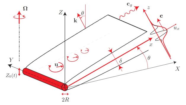
Figure 1: Geometry of an inertial wave beam emitted in an infinite medium from a localized oscillating cylindrical wavemaker invariant in the $Y$-direction.

II.2 Viscous spreading

In a viscous fluid, the energy of the wave beam is dissipated because of the shearing motion between oscillating planes. As the energy propagates away from the source, the larger wavenumbers will be damped first, so that the spectrum of the wave beam gradually concentrates towards lower wavenumbers, resulting in a spreading of the wave beam away from the source.

Although the viscous attenuation of a single Fourier component yields a purely exponential decay, the attenuation of a localized wave follows a power law with the distance from the source, which originates from the combined exponential attenuation of its Fourier components. A similarity solution for the viscous spreading of a wave beam has been derived by Thomas and StevensonThomas1972 in the case of internal waves, and has been extended to the case of coupled internal-inertial waves by Peat.Peat1978 The derivation in the case of a pure inertial wave is detailed in the Appendix, and we provide here only a qualitative argument for the broadening of the wave beam.

During a time $t$, the amplitude of a planar monochromatic wave of wavevector ${\bf k}$ is damped by a factor $\epsilon_{k}=\exp(-\nu k^{2}t)$ as it travels of a distance $x=c_{g}t$ along the beam, where $c_{g}$ is the group velocity. Using $c_{g}=(2\Omega/k)\sin\theta=(\sigma/k)\tan\theta$, the attenuation factor writes

$$\epsilon_{k}=\exp(-\ell^{2}k^{3}x),$$

where we introduce the viscous lengthscale,

$$\ell=\left(\frac{\nu}{\sigma\tan\theta}\right)^{1/2}.$$ (2)

For a wave beam emitted from a thin linear source at $x=0$, an infinite set of plane waves are generated, and the energy of the largest wavenumbers will be preferentially attenuated as the wave propagates in the $x$ direction. At a distance $x$ from the source, the largest wavenumber, for which the energy has decayed by less than a given factor $\epsilon^{*}$, is $k_{max}=(\ell^{2}x)^{-1/3}\ln\epsilon^{*}$. At this distance $x$, the wave beam thus results from the interference of the remaining plane waves of wavenumbers ranging from 0 to $k_{max}$. Its thickness can be approximated by $\delta(x)\sim k_{max}^{-1}$, yielding $\delta(x)/\ell\sim(x/\ell)^{1/3}$. Mass conservation across a surface normal to the group velocity implies that the velocity amplitude of the wave must decrease as $x^{-1/3}$.

More specifically, introducing the reduced transverse coordinate $\eta=z/x^{1/3}\ell^{2/3}$, a similarity solution exists for the velocity envelope,

$$u_{0}(x)=U_{0}^{*}\frac{E_{0}(\eta)}{E_{0}(0)}\left(\frac{\ell}{x}\right)^{1/3},$$ (3)

where $U_{0}^{*}$ is the velocity scale of the wave, and the analytical expression of the non-dimensional envelope $E_{0}(\eta)$ is given in the Appendix. Similarly, the vorticity envelope can be written as

$$\omega_{0}(x)=W_{0}^{*}\frac{E_{1}(\eta)}{E_{1}(0)}\left(\frac{\ell}{x}\right)^{2/3},$$ (4)

with $W_{0}^{*}$ the vorticity scale. Although the normalized velocity envelope $E_{0}(\eta)/E_{0}(0)$ has larger tails than the vorticity one $E_{1}(\eta)/E_{1}(0)$, they turn out to be almost equal for $\eta<4$. The width at mid-height, defined such that $E_{m}(\eta_{1/2}/2)=E_{m}(0)/2$, with $m=0,1$, is $\eta_{1/2}\simeq 6.84$ for both envelopes, so that the width of the beam in dimensional units is

$$\delta(x)\simeq 6.84\,\ell\left(\frac{x}{\ell}\right)^{1/3}.$$ (5)

II.3 Finite size effect of the source

The similarity solution described here applies only in the case of a source of size much smaller than the viscous scale $\ell$. In the case of internal waves, Hurley and KeadyHurley1997 (see also Flynn et al.Flynn2003 ) have shown that for a source of large extent, vertically vibrated with a small amplitude, the wave could be approximately described as originating from two virtual sources, respectively located at the top and bottom of the disturbance. Following qualitatively this approach in the case of inertial waves forced by a horizontal cylinder of radius $R$, the boundaries of the upper wave are given by $z_{\mathrm{up}}^{\pm}=R\pm\delta(x)/2$, and that of the lower wave are given by $z_{\mathrm{down}}^{\pm}=-R\pm\delta(x)/2$. The lower boundary of the upper source intersects the upper boundary of the lower source at a distance $x_{i}$ such that $z_{\mathrm{up}}^{-}(x_{i})=z_{\mathrm{down}}^{+}(x_{i})$, yielding

$$\frac{x_{i}}{R}\simeq 0.025\,\left(\frac{R}{\ell}\right)^{2}.$$ (6)

For large wavemakers ($R/\ell\gg 0.025^{-1/2}\simeq 6.3$), one has two distinct wave beams for $x\ll x_{i}$, and one single merged beam for $x\gg x_{i}$. On the other hand, for smaller wavemakers, the merging of the two wave beams occur virtually inside the source, which can be effectively considered as a point source. In this case, the effective beam width far from the source may be simply written as

$$\delta_{\mathrm{eff}}(x)\simeq 2R+\delta(x).$$ (7)

III The experiment

III.1 Experimental setup

The experimental setup consists in a cubic glass tank, of sides $60$ cm and filled with 54 cm of water (see Fig. 2), mounted on the new precision rotating turntable “Gyroflow”, of 2 m in diameter. The angular velocity $\Omega$ of the turntable is set in the range 0.63 to 2.09 rad s^-1, with relative fluctuations $\Delta\Omega/\Omega$ less than $5\times 10^{-4}$. A cover is placed at the free surface, preventing from disturbances due to residual surface waves. The rotation of the fluid is set long before each experiment in order to avoid transient spin-up recirculation flows and to achieve a clean solid body rotation.

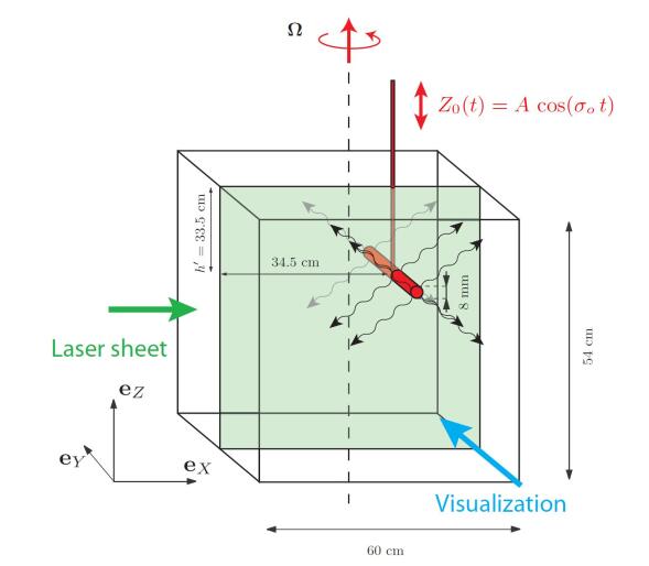
Figure 2: Schematic view of the experimental setup. The horizontal 8 mm diameter cylinder is oscillating vertically according to $Z_{0}(t)=A\,\cos(\sigma_{o}\,t)$, with $A=2$ mm and $\sigma_{o}=0.2$ Hz. PIV measurements in a vertical plane ($X$,$Z$) in the rotating frame are achieved by a vertical laser sheet and a camera at $90^{\circ}$.

The wavemaker is a horizontal cylinder of radius $R=4$ mm and length $L=50$ cm, hung at $33.5$ cm below the cover by a thin vertical stem of 3 mm diameter. It is off-centered in order to increase the size of the studied wave beam in the quadrant $X<0$ and $Z<0$. The vertical oscillation $Z_{0}(t)=A\,\cos(\sigma_{o}t)$, with $A=2$ mm, is achieved by a step-motor, coupled to a circular camshaft which converts the rotation into a sinusoidal vertical oscillation. In the present experiments, the wavemaker frequency is kept constant, equal to $\sigma_{o}=1.26$ rad s^-1, and the angular velocity of the turntable is used as the control parameter. This allows the velocity disturbance $\sigma_{o}\,A=2.5$ mm s^-1 to be fixed, whereas the angle of the inertial wave beam with respect to the horizontal, $\theta=\cos^{-1}(\sigma_{o}/2\Omega)$, is varied between 0 and 72^o. The velocity and vorticity profiles are examined at distances $x$ between 30 and 300 mm from the wavemaker. The three-dimensional effects originating from the finite size $L$ of the cylinder can be safely neglected since $x<0.6L$. The Reynolds number based on the wavemaker velocity is $Re=\sigma_{o}A(2R)/\nu\simeq 20$, so that the flow in the vicinity of the wavemaker is essentially laminar. Except in Sec. IV.2, where the transient regime is described, measurements start after several wavemaker periods in order to achieve a steady state.

For the forcing frequency $\sigma_{o}$ considered here, the boundary layer thickness is $\delta_{S}=(\nu/\sigma_{o})^{1/2}\simeq 0.9$ mm. This thickness also gives the order of magnitude of the viscous length $\ell=\delta_{S}/\sqrt{\tan\theta}$ [see Eq. (2)], for angles not too close to 0 and $\pi/2$. The wavemaker radius being chosen such that $R/\ell\simeq 4$, the small source approximation is satisfied according to the criterion discussed in Sec. II.3.

III.2 PIV measurements

Velocity fields in a vertical plane ($X$,$Z$) are measured using a 2D Particle Image Velocimetry system. The flow is seeded by 10 $\mu$m tracer particles, and illuminated by a vertical laser sheet, generated by a 140 mJ Nd:YAg pulsed laser. A vertical $43\times 43$ cm² field of view is acquired by a $2048\times 2048$ pixels camera synchronized with the laser pulses. The field of view is set on the lower left wave beam. For each rotating rate, a set of 2000 images is recorded, at a frequency of 2 Hz, representing 10 images per wavemaker oscillation period.

PIV computations are performed over successive images, on $32\times 32$ pixels interrogation windows with $50\%$ overlap, leading to a spatial resolution of 3.4 mm.DaVis In the following, the two quantities of interest are the velocity component $u_{x}$, obtained from the measured components $u_{X}$ and $u_{Z}$ projected along the direction of the wave beam, and the vorticity component $\omega_{y}$, normal to the measurement plane.

The velocity along the wave beam typically decreases from 1 to 0.1 mm s^-1, and is measured with a resolution of 0.02 mm s^-1. Two sources of velocity noise are present, both of order of 0.2 mm s^-1, originating from residual modulations of the angular velocity of the turntable, and from thermal convection effects due to a slight difference between the water and the room temperature. The residual velocity modulations, of order of $L_{0}\,\Delta\Omega/2$ (where $L_{0}$ is the tank size and $\Delta\Omega\simeq 5\times 10^{-4}\Omega$) are readily removed by computing the phase-averaged velocity fields over the 200 periods of the wavemaker. Thermal convective motions, in the form of slowly drifting ascending and descending columns, could be reduced but not completely suppressed by this phase-averaging, and represent the main source of uncertainty in these experiments. However, the vorticity level associated to those convective motions appears to be negligible compared to the typical vorticity of the inertial wave. Therefore, the vorticity profiles of the wave could be safely computed from the phase-averaged velocity fields.

IV General properties of the wave pattern

IV.1 Visualisation of the wave beams

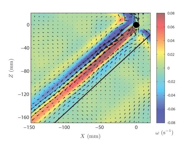
Figure 3: Close-up view of the phase averaged velocity (arrows) and vorticity $\omega_{y}$ (color mapped) for an experiment performed at $\sigma_{o}/2\Omega=0.67$. The black line shows the direction predicted by the dispersion relation $\cos\theta=\sigma_{o}/2\Omega$.

Figure 3 is a close-up view of the velocity and vorticity fields at $\sigma_{o}/2\Omega=0.67$, showing the vorticity layers of alternating sign where the measured velocity is almost parallel to the ray direction ${\bf e}_{x}$. The angle of the ray with respect to the horizontal accurately follows the prediction of the dispersion relation (1), as illustrated by the black line. In Fig. 4(a) to (c), phase-averaged horizontal vorticity fields $\omega_{y}$ are shown for three regularly sampled values of the phase. One can clearly see the location of the inertial wave inside a wavepacket that draws the classical four-rays St. Andrew’s cross. The evolution of the vorticity field from Fig. 4(a) to (c) illustrates the propagation of the phase in directions normal to the rays. Some reflected wave beams of much smaller amplitude may also be distinguished on the background.

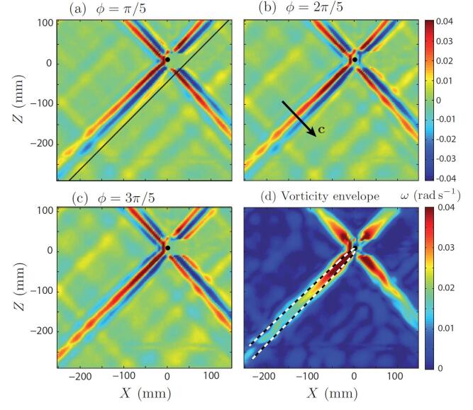
Figure 4: Phase averaged horizontal vorticity field $\omega_{y}$ for $\sigma_{o}/2\Omega=0.67$ at different phases: (a) $\phi=\pi/5$, (b) $\phi=2\pi/5$ and (c) $\phi=3\pi/5$. The black line in (a) draws the direction predicted by the dispersion relation. (d) Vorticity envelope field $\omega_{0}$ (see Sec. V). The dashed black and white lines shows the wave beam thickness predicted by the similarity solution [see Eq. (7)].

Figure 5 compares the cosine of the measured angle $\theta$ with the theoretical value $\sigma_{o}/2\Omega$ according to the prediction of the dispersion relation (1). The angle is determined from the location of the maximum of the vorticity envelope (envelope computations described in Sec. V), shown in Fig. 4(d), averaged along the ray. An excellent agreement is obtained between the measurements and the theory, with a relative error less than $3\%$.

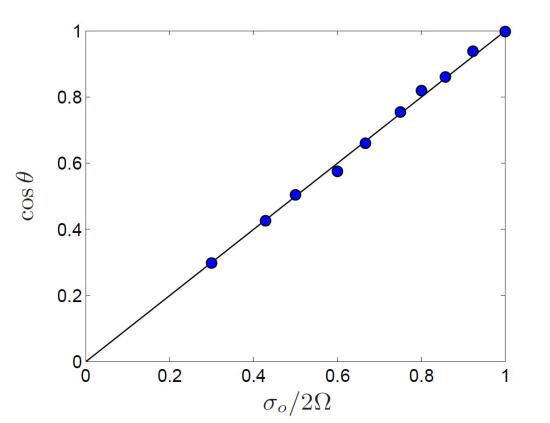
Figure 5: Cosine of the measured average beam angle, $\cos\theta$, as a function of the frequency ratio $\sigma_{o}/2\Omega$. The line shows the dispersion relation (1). Experimental uncertainties are of the order of the marker size.

IV.2 Transient experiments

In order to characterize the formation of the inertial wave pattern as the oscillation is started, a series of transient experiments has been performed. In the case of a pure monochromatic plane wave, the front velocity of the wavepacket is simply given by the group velocity. However, in the case of a localized wave beam, since each Fourier component $k$ travels with its own group velocity $c_{g}=(\sigma/k)\tan\theta$, the shape of the wavepacket gradually evolves as the wave propagates. A rough estimate for the front velocity can be simply obtained from $V_{f}\simeq\sigma(\lambda/2\pi)\tan\theta$, where $\lambda$ is the apparent wavelength of the wave, simply estimated as twice the distance between the locations of two successive vorticity extrema.

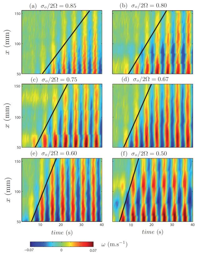
Figure 6: Spatiotemporal representation of the vorticity $\omega_{y}$ along the wave beam, where space is the distance $x$ to the oscillating cylinder, for experiments performed at $\sigma_{o}/2\Omega=0.85,\,0.80,\,0.75,\,0.66,\,0.60,\,0.50$. Black lines originating at ($x=0,t=0$) trace the front velocity $V_{f}=\sigma(\lambda/2\pi)\tan\theta$ estimated from the apparent wavelength (see Sec. V.1). $t=0$ corresponds to the start of the oscillation.

Figure 6 shows spatiotemporal diagrams of the vorticity $\omega_{y}(x,z=0,t)$ at the center of the beam as a function of the distance $x$ from the wavemaker, for $\sigma_{o}/2\Omega$ between 0.85 and 0.50. Superimposed to these spatiotemporal images, we show the front velocity $V_{f}\simeq\sigma(\lambda/2\pi)\tan\theta$, starting from $x=0$ at $t=0$. Qualitative agreement with the spatiotemporal diagrams is obtained, indicating that the propagation of the wave envelope is indeed compatible with this front velocity.

Further quantitative estimate of the front velocity would require to extract the instantaneous wave envelope from those spatio-temporal diagrams, which is difficult because the front velocity and the phase velocity are of the same order. This property actually prevents from a safe extraction of a longitudinal wavepacket envelope using standard temporal averaging over small time windows.

IV.3 Generation of harmonics

Going back to steady waves, we now characterize the generation of higher order wave beams which take place at low forcing frequency. According to the dispersion relation, an harmonic wave of order $n\geq 2$ is allowed to develop whenever $n\sigma_{o}/2\Omega<1$. Such harmonic waves of order $n\geq 2$ may originate either from a residual non-harmonic component of wavemaker oscillation profile $Z_{0}(t)$, or from inertial non-linear effects in the flow in the vicinity of the wavemaker, which can exist at the Reynolds number $Re\simeq 20$ considered here.

In Fig. 4, in which $\sigma_{o}/2\Omega=0.67$, only the fundamental wave ($n=1$) can be seen. On the other hand, in Fig. 7(a), in which $\sigma_{o}/2\Omega=0.43$, a second harmonic wave beam is clearly present, propagating at an angle closer to the horizontal, as expected from the dispersion relation. This is confirmed by Fig. 7(b) and (c), showing the corresponding frequency-filtered phase averaged vorticity fields, in (b) for the fundamental $n=1$ and in (c) for the second harmonics $n=2$.

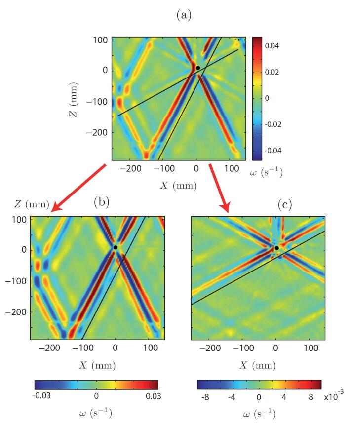
Figure 7: (a) Phase averaged vorticity field $\omega_{y}$ for an experiment performed at $\sigma_{o}/2\Omega=0.43$, showing both the fundamental ($n=1$) and the second harmonic ($n=2$) wave beams. The corresponding frequency-filtered vorticity fields are extracted in (b) and (c).

In order to further characterize this generation of harmonics, we have performed a spectral analysis of the time series of the longitudinal velocity $u_{x}(t)$, measured at a given distance $x_{0}=100$ mm from the source, at the center of each wave beam. The energy spectrum $|\hat{u}_{\sigma}|^{2}$, where $\hat{u}_{\sigma}$ is the temporal Fourier transform of $u_{x}(t)$, is shown in Fig. 8 for the two cases $\sigma_{o}/2\Omega=0.67$ and $0.43$. In both cases, the spectra are clearly dominated by the fundamental forcing frequency $\sigma_{o}$. Two other peaks are also found, at $\sigma=\Omega$ and $\sigma=2\Omega$, originating from the residual modulation of the angular velocity of the platform, as discussed in Sec. III.2 (the energy of those peaks is typically 3 to 10 times smaller than the fundamental one). As expected, no harmonic frequency $n\sigma_{o}$ ($n\geq 2$) is found for $\sigma_{o}/2\Omega=0.67$ (see Fig. 8a), but a second harmonic $n=2$ is indeed present for $\sigma_{o}/2\Omega=0.43$ (see Fig. 8b). In this case, the energy ratio of the first to the second harmonics, each of them being measured at a distance $x_{0}=100$ mm from the source on the corresponding beam, is $|\hat{u}_{2\sigma}|^{2}/|\hat{u}_{\sigma}|^{2}\simeq 0.036$. As $\sigma_{o}/2\Omega$ is further decreased, the ratio $|\hat{u}_{2\sigma}|^{2}/|\hat{u}_{\sigma}|^{2}$ increases, reaching $0.05$ for $\sigma_{o}/2\Omega=0.30$, and even higher order harmonics emerge although with very weak amplitude.

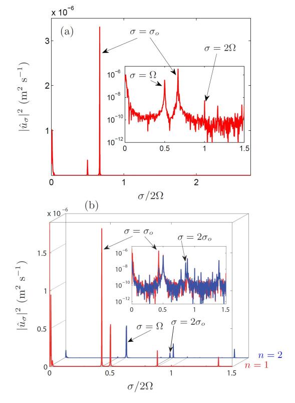
Figure 8: Energy spectrum of the velocity time series measured at the center of the wave beam of interest, at a fixed distance $x_{0}=100$ mm from the wavemaker. (a) $\sigma_{o}/2\Omega=0.67$, showing a single peak at the forcing frequency. (b) $\sigma_{o}/2\Omega=0.43$, showing measurements performed in the fundamental beam $n=1$ (in red/light gray) and in the second harmonic beam $n=2$ (in blue/dark gray). In (a) and (b), insert shows the same spectrum in semi-logarithmic coordinates. Additional peaks are present at $\sigma/2\Omega=0.5$ and $1$, originating from mechanical noise of the rotating platform.

V Test of the similarity solution

V.1 Velocity and vorticity envelopes

We now focus on the dependence of the wavepacket shape and the viscous spreading of the wave beam with the distance $x$ from the source. Figures 9(a) and (b) illustrate the shape of the phase-averaged velocity and vorticity profiles respectively, for two values of the phase $\phi_{0}$ and $\phi_{0}+2\pi/5$. The wavepacket envelopes are defined as

$$u_{0}(x,z)=\sqrt{2\langle u_{x}(x,z,\phi)^{2}\rangle_{\phi}}$$

(and similarly for $\omega_{0}$), where $\langle\cdot\rangle_{\phi}$ is the average over all phases $\phi$. Although the measured normalized envelopes compare well with the normalized envelopes predicted from the similarity solutions [$E_{m}(\eta)/E_{m}(0)$, with $m=0$ for the velocity and $m=1$ for the vorticity], the agreement is actually better for the vorticity. This is probably due to the velocity contamination originating from the residual angular velocity modulation of the platform and the slight thermal convection effects discussed in Sec. III.2. The better defined vorticity envelopes actually confirms that those velocity contaminations have a negligible vorticity contribution. For this reason, we will concentrate only on the vorticity field in the following.

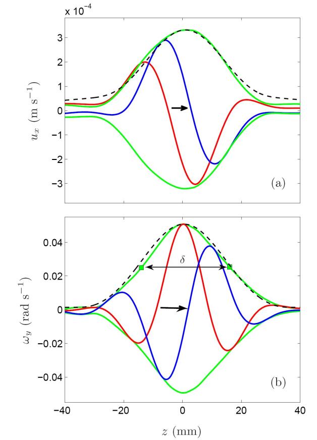
Figure 9: (a) Velocity envelope $u_{0}(x_{0},z)$ and two velocity profiles $u_{x}(x_{o},z,\phi)$ for two values of the phase $\phi$, as a function of the transverse coordinate $z$ at a fixed distance $x_{o}=100$ mm from the wavemaker for $\sigma_{o}/2\Omega=0.67$. (b) Corresponding vorticity envelope $\omega_{0}(x_{0},z)$ and vorticity profiles $\omega_{y}(x_{0},z,\phi)$. $\delta$ is the envelope thickness at mid-height. In (a) and (b), the green/light gray curves correspond to the experimental envelope, and the dotted curves correspond to the predictions of the similarity solutions normalized by the measured maximum.

It is worth to examine here the singular situation $\sigma_{o}/2\Omega=1$, in which the similarity solution is no longer valid. In this situation, the phase velocity is strictly vertical and the group velocity vanishes. The upward and downward beams are expected to superimpose and generate a stationary wave pattern in the horizontal plane $Z=z=0$. Figure 10 shows the velocity envelope $u_{0}(x_{0},z)$ and three phase averaged profiles as a function of the transverse coordinate $z$. The observed wave is actually stationary at the center of the wavepacket (see the velocity node and vorticity maximum for $z=0$), and shows outwards propagations on each side of the wavepacket.

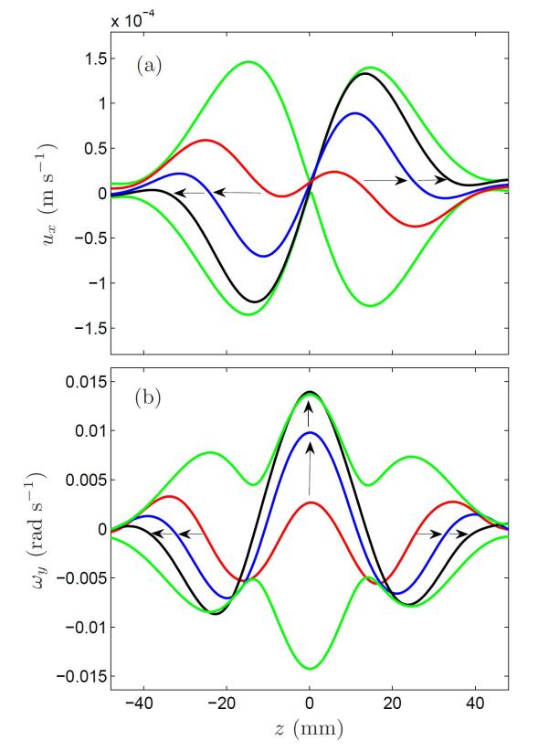
Figure 10: (a) Velocity envelope $u_{0}(x_{0},z)$ and three velocity profiles $u_{x}(x_{0},z,\phi)$ as a function of the transverse coordinate $z$ at a fixed distance $x_{o}=70$ mm from the wavemaker for $\sigma_{o}/2\Omega=1$. (b) Corresponding vorticity envelope and vorticity profiles. The arrows indicate the time evolution of the profiles. The interference of the upward and downward wave beams produces a stationary wave pattern at $z=0$ with a velocity node and a vorticity maximum.

Returning to the standard situation $\sigma_{o}/2\Omega<1$, the vorticity amplitude at a given location $x$ is defined as the maximum of the vorticity envelope at the center of the beam, $\omega_{max}(x)=\omega_{0}(x,z=0)$. The thickness of the wavepacket $\delta(x)$ is defined from the width at mid-height of the envelope, such that

$$\omega_{0}(x,\delta(x)/2)=\omega_{max}(x)/2.$$

This beam thickness $\delta$ depends both on the distance $x$ from the source and on the viscous length $\ell$ [see Eqs. (5) and (7)]. In order to check those two dependencies, $\delta$ is plotted in Fig. 11(a) as a function of $x$ at fixed $\sigma_{o}/2\Omega$, and in Fig. 11(b) as a function of $\sigma_{o}/2\Omega$ at fixed $x_{0}$. The agreement with the effective wave beam thickness $\delta_{\rm eff}=2R+6.84\ell(x/\ell)^{1/3}$ is correct, to within $10\%$, which justifies the simple analysis of merged beams originating from the two virtual sources located at the top and bottom of the wavemaker. The oscillations of $\delta$ probably originate from the interaction of the principal wave beam with reflected ones. Figure 11(a) also shows the apparent wavelength $\lambda(x)$ of the wave, simply defined as twice the distance between a maximum and a minimum of the phase-averaged vorticity profiles. This apparent wavelength turns out to be even closer to the expected lengthscale $\delta_{\rm eff}$ of Eq. (7), to within $4\%$, suggesting that $\lambda$ is less affected by the background noise than the beam thickness. A good agreement between both $\delta$ and $\lambda$ and the prediction (7) is also obtained as $\sigma_{o}/2\Omega$ (and hence $\ell$) is varied at fixed $x_{0}$, as shown in Fig. 11(b). Here again, the interaction with reflected wave beams is probably responsible for the significant scatter in this figure.

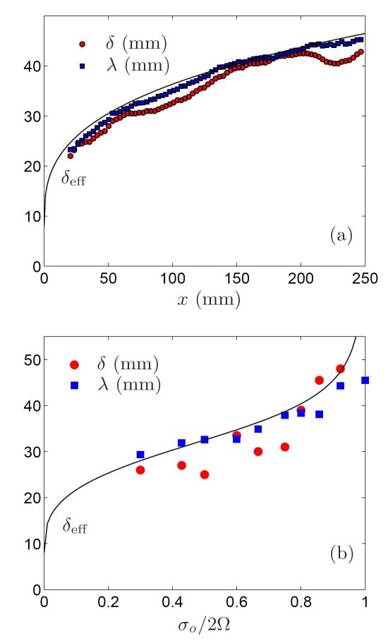
Figure 11: Wave beam thickness $\delta$ (red $\circ$), and apparent wavelength $\lambda$ (blue $\square$); (a), as a function of the distance $x$ from the wavemaker for $\sigma_{o}/2\Omega=0.67$; (b), as a function of $\sigma_{o}/2\Omega$ at a distance $x_{o}=100$ mm from the wavemaker. In both plots, the line shows the predicted effective wave beam thickness $\delta_{\mathrm{eff}}$ (7).

V.2 Decay of the vorticity envelope

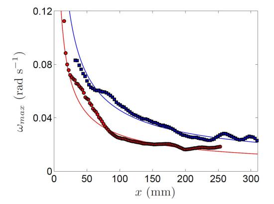
Figure 12: Vorticity amplitude $\omega_{max}(x)$ as a function of the distance $x$ from the wavemaker for $\sigma_{o}/2\Omega=0.67$ (blue $\square$) and $\sigma_{o}/2\Omega=0.85$ (red $\circ$), and best fit with the law $W_{0}^{*}(x/\ell)^{-2/3}$.

The decay of the vorticity amplitude $\omega_{max}(x)$ as a function of the distance $x$ from the source is shown in Fig. 12. Taking the similarity solution (4) at the center of the wave beam $z=0$ yields

$$\omega_{max}(x)=W_{0}^{*}\,\left(\frac{\ell}{x}\right)^{2/3}.$$ (8)

Letting the vorticity scale $W_{0}^{*}$ as a free parameter, a power law $x^{-2/3}$ is found to provide a good fit for the overall decay of $\omega_{max}(x)$. Some marked oscillations are however clearly visible, e.g. at $x$ between 220 and 320 mm for $\sigma_{o}/2\Omega=0.85$ (blue $\square$ in Fig. 12). Those oscillations appear at locations where reflected wave beams interact with the principal one, inducing modulations of the wave amplitude. This interpretation is confirmed by the fact that (i) the observed modulation has a wavelength of $45$ mm, which corresponds to the apparent wavelength of the wave, and that (ii) in Fig. 4, corresponding to $\sigma_{o}/2\Omega=0.67$, a modulation of the principal wave beam by a reflected can be clearly seen at a distance of about $250$ mm from the source.

The vorticity scale $W_{0}^{*}$ is theoretically related to the velocity scale $U_{0}^{*}$ through the relation $W_{0}^{*}=(E_{1}(0)/E_{0}(0))U_{0}^{*}/\ell\simeq 0.506\,U_{0}^{*}/\ell$ (see the Appendix). Since the wavemaker velocity is $\sigma_{o}A$, the velocity scale $U_{0}^{*}$ is expected to write in the form $\sigma_{o}A\,g(\theta)$, where the unknown function $g(\theta)$ describes the forcing efficiency of the wavemaker. Accordingly, the forcing efficiency can be deduced from the vorticity data, by computing

$$g(\theta)=\frac{W_{0}^{*}}{0.506\,\sigma_{o}A/\ell}=\frac{\omega_{max}\,(x/\ell)^{2/3}}{0.506\,\sigma_{o}A/\ell}$$ (9)

for each value of $\sigma_{o}/2\Omega$. Measurements of $g(\theta)$ are plotted as a function of $\sigma_{o}/2\Omega$ in Fig. 13. As expected, this forcing efficiency decreases as $\sigma_{o}/2\Omega$ is increased, i.e. as the wave beam becomes closer to the horizontal. In the limit $\sigma_{o}/2\Omega\rightarrow 1$, the vertically oscillating wavemaker becomes indeed very inefficient to force the quasi-horizontal velocities of the wave.

An analytical expression for the function $g(\theta)$ would require to solve exactly the velocity field in the vicinity of the wavemaker, and in particular the coupling between the oscillating boundary layer and the wave far from the source, which is beyond the scope of this paper. In the case of a cylinder, a naive estimate of $g(\theta)$ could however be obtained, assuming that the effective velocity forcing is simply given by the projection of the wavemaker velocity along the wave beam direction, yielding

$$g(\theta)=g_{0}\sin\theta=g_{0}\,\sqrt{1-\left(\frac{\sigma_{o}}{2\Omega}\right)^{2}},$$ (10)

with $g_{0}$ a constant to be determined. A best fit of the experimental values of $g(\theta)$ with this law leads to $g_{0}\simeq 0.94\pm 0.10$ [see Fig. 13], and reproduces well the decrease of $g(\theta)$ as $\sigma_{o}/2\Omega$ is increased. The fact that $g_{0}$ is found close to 1 indicates that the inertial wave beam is essentially fed by the oscillating velocity field in the close vicinity of the wavemaker. The discrepancy at large forcing frequency may be due to the breakdown of the similarity solution as the angle $\theta$ approaches $0$.

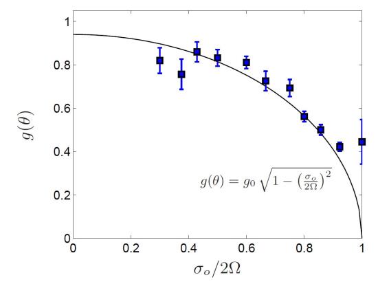
Figure 13: Forcing efficiency $g(\theta)$ defined from Eq. (9) as a function of $\sigma_{o}/2\Omega$. Squares and errorbars represents respectively the mean and the standard deviation for each $\sigma_{o}/2\Omega$ ratio (reflecting the variability of $\omega_{max}$ along $x$). The black line shows a best fit according to Eq. (10), with $g_{0}=0.94\pm 0.10$.

VI Stokes drift

We finally consider the possibility of a Stokes drift along the wavemaker which is expected because of the attenuation of the wave amplitude induced by the viscosity. A fluid particle in the inertial wave approximately describes a circular orbit. During this orbit, the particle experiences a larger velocity along $y$ when it is closer than when it is further from the wavemaker (see Fig. 1), resulting in a net mass transport along $y$. This is similar to the classical Stokes drift for water waves, which is horizontal because of the decay of the velocity magnitude with depth.Longuet1953 Here the drift is expected in general in the direction given by $\boldsymbol{\Omega}\times{\bf c}_{g}$, since the viscous attenuation takes place along the group velocity ${\bf c}_{g}$.

Attempts to detect this effect have been carried out, from PIV measurements in vertical planes $(Y,Z)$. Because of the weakness of the considered drift, the measurements have been performed very close to the wavemaker, for $X$ between 5 and 30 mm, where a stronger effect is expected. However, those attempts were not successful, probably because the drift, if present, is hidden by the stronger fluid motions induced by the residual thermal convection columns, as discussed in Sec. III.2.

The magnitude of the expected Stokes drift cannot be easily inferred from the complex motion of the fluid particles close to the wavemaker. An estimate could however be obtained in the far field, from the similarity solution of the wave beam. We consider for simplicity a particle lying at the center of the wave beam ($z=0$), at a mean distance $x_{0}$ from the source, describing approximate circles of gyration radius $a\simeq|{\bf u}(x_{0})|/\sigma$ in the tilted plan $(x,y)$. The expected drift velocity $\overline{\bf v}_{S}$ can be approximated by computing the velocity difference between the two extreme points $x_{0}-a$ and $x_{0}+a$ of the orbit, yielding, to first order in $a/x_{0}$ to,coeffdrift

$$\overline{v}_{Sy}(x_{0})\simeq\frac{2}{3}\frac{U_{0}^{*2}\ell^{2/3}}{\sigma x_{0}^{5/3}}.$$ (11)

The steep decrease as $x_{0}^{-5/3}$ confirms that the drift should be essentially present close to the wavemaker. Although this formula is expected to apply only in the far-field wave (typically for $x_{0}>40\ell$, see the Appendix), its extrapolation close to the wavemaker, for $x_{0}\simeq 10\ell\simeq 2R$, gives $\overline{v}_{Sy}\simeq 0.1$ mm s^-1. This expected drift velocity is about 10% of the wave velocity at the same location, but it turns out to remain smaller than the velocity contamination due to the thermal convection columns. Although the phase averaging proved to be efficient to extract the inertial wave field from the measured velocity field – thanks to a frequency separation between convection effects and inertial wave –, it fails here to extract the much weaker velocity signal expected from this drift, since it is zero frequency and hence mixed with the very low frequency convective noise.

VII Conclusion

In this paper, Particle Image Velocimetry measurements have been used to provide quantitative insight into the structure of the inertial wave emitted by a vertically oscillating horizontal cylinder in a rotating fluid. Large vertical fields of view could be achieved thanks to a new rotating platform, allowing for direct visualization of the cross-shaped St. Andrew’s wave pattern.

It must be noted that performing accurate PIV measurements of the very weak signal of an inertial wave is a challenging task. In spite of the high stability of the angular velocity of the platform ($\Delta\Omega/\Omega<5\,10^{-4}$), the velocity signal-to-noise remains moderate here. Additionally, slowly drifting vertical columns are present because of residual thermal convection effects, and are found to account for most of velocity noise in these experiments. Those thermal convection effects are very difficult to avoid in large containers, even in an approximately thermalized room. However, this noise can be significantly reduced by a phase-averaging over a large number of oscillation periods. This concern is not present for internal waves in stratified fluids, because residual thermal motions are inhibited by the stable stratification. This emphasizes the intrinsic difficulty of experimental investigation of inertial waves, in contrast to internal waves which have been the subject of a number of studies.

In this article, emphasis has been given on the spreading of the inertial wave beam induced by viscous dissipation. The attenuation of a two-dimensional wave beam emitted from a linear source is purely viscous, whereas it combines viscous and geometrical effects in the case of a conical wave emitted from a point source. The linear theory presented in this paper is derived under the classical boundary-layer assumptions first introduced by Thomas and StevensonThomas1972 for two-dimensional internal waves in stratified fluids. The measured thickening of the wave beam and the decay of the vorticity envelope are quantitatively fitted by the scaling laws of the similarity solutions of this linear theory, $\delta(x)\sim x^{1/3}$ and $\omega_{max}(x)\sim x^{-2/3}$, where $x$ is the distance from the source. More precisely, we have shown that the amplitude of the vorticity envelope could be correctly predicted from the velocity disturbance induced by the wavemaker, by introducing a simple forcing efficiency function $g(\theta)$, where $\theta$ is the angle of the wave beam.

Finally, it is shown that an attenuated inertial wave beam should in principle generate a Stokes drift along the wavemaker, in the direction given by $\boldsymbol{\Omega}\times{\bf c}_{g}$, where ${\bf c}_{g}$ is the group velocity. However, in spite of the high precision of the rotating platform and the PIV measurements, attempts to detect this drift were not successful in the present configuration. Velocity fluctuations induced by thermal convection effects probably hide this slight mean drift velocity, suggesting that an improved experiment with a very carefully controlled temperature stability would be necessary to detect this very weak effect.

Appendix A Similarity solution for a viscous planar inertial wave

In this appendix, we derive the similarity solution for a viscous planar inertial wave, following the procedure first described by Thomas and StevensonThomas1972 for internal waves.

We consider the inertial wave emitted from a thin linear disturbance invariant along the $Y$ axis and oscillating along $Z$ with a pulsation $\sigma$ in a viscous fluid rotating at angular velocity ${\boldsymbol{\Omega}}=\Omega{\bf e}_{Z}$. Since the linear source is invariant along $Y$, so will the wave beams, and the energy propagates in the $(X,Z)$ plan. In the following, we consider only the wave beam propagating along $X>0$ and $Z>0$.

The linearized vorticity equation is

$$\partial_{t}{\boldsymbol{\omega}}=(2{\boldsymbol{\Omega}}\cdot\nabla){\bf u}+\nu\nabla^{2}{\boldsymbol{\omega}}.$$

Recasting the problem in the tilted frame of the wave, $({\bf e}_{x},{\bf e}_{y},{\bf e}_{z})$, with ${\bf e}_{y}={\bf e}_{Y}$, and ${\bf e}_{x}$ tilted of an angle $\theta=\cos^{-1}(\sigma/2\Omega)$ with the horizontal, one has ${\boldsymbol{\Omega}}=\Omega\,(\sin\theta\,{\bf e}_{x}+\cos\theta\,{\bf e}_{z})$, so that $(2{\boldsymbol{\Omega}}\cdot\nabla)=2\Omega\,(\sin\theta\,\partial_{x}+\cos\theta\,\partial_{z})=\sigma\,(\tan\theta\,\partial_{x}+\partial_{z})$. Assuming that the flow inside the wave beam is quasi-parallel (boundary layer approximation), i.e., such that $|u_{x}|,|u_{y}|\gg|u_{z}|$, $|\omega_{x}|,|\omega_{y}|\gg|\omega_{z}|$, and $\nabla^{2}\simeq\partial_{z}^{2}$, the linearized vorticity equation reduces to

$$\partial_{t}\omega_{x} = \sigma(\tan\theta\partial_{x}+\partial_{z})u_{x}+\nu\partial_{z}^{2}\omega_{x},$$ (12)

$$\partial_{t}\omega_{y} = \sigma(\tan\theta\partial_{x}+\partial_{z})u_{y}+\nu\partial_{z}^{2}\omega_{y}.$$ (13)

We introduce the complex velocity and vorticity fields in the $(x,y)$ plan as

$$U=u_{x}+iu_{y},\qquad W=\omega_{x}+i\omega_{y}.$$

Since, within the quasi-parallel approximation, one has $W=i\partial_{z}U$, the combination (12)$+i$(13) yields

$$i\partial_{t}\partial_{z}U=\sigma(\tan\theta\partial_{x}+\partial_{z})U+i\nu\partial_{z}^{3}U.$$ (14)

Searching solutions in the form $U=U_{0}e^{-i\sigma t}$, Eq. (14) becomes

$$\partial_{x}U_{0}+i\ell^{2}\partial_{z}^{3}U_{0}=0,$$ (15)

where we have introduced the viscous scale $\ell$ (2). Eq. (15) admits similarity solutions as a function of the variable:

$$\eta=\frac{z}{x^{1/3}\ell^{2/3}},$$ (16)

which are of the form:

$$U_{0}(x,z)=\tilde{U}_{0}\left(\frac{\ell}{x}\right)^{1/3}f(\eta),$$ (17)

and where $\tilde{U}_{0}$ is a velocity scale and $f(\eta)$ a non-dimensional complex function of the reduced transverse coordinate $\eta$. Plugging such similarity solution (17) into Eq. (15) shows that $f(\eta)$ is solution of the ordinary differential equation

$$3f^{\prime\prime\prime}+i(f+\eta f^{\prime})=0,$$ (18)

which is identical to the equation (16) derived by Thomas and StevensonThomas1972 for the pressure field of internal waves. Following their development, we introduce the family of functions $f_{m}$ defined through

$$f_{m}(\eta)=c_{m}+is_{m}=\int_{0}^{\infty}K^{m}e^{-K^{3}}e^{iK\eta}dK,$$ (19)

where $c_{m}$ and $s_{m}$ are real, and such that $f_{0}(\eta)$ is a solution of Eq. (18).

The velocity in the plan of the wave beam is therefore given by $u_{x}=\Re\{U\}$ and $u_{y}=\Im\{U\}$, leading to

$$u_{x}=\frac{U_{0}^{*}}{E_{0}(0)}\left(\frac{\ell}{x}\right)^{1/3}\left[c_{0}(\eta)\cos(\sigma t)+s_{0}(\eta)\sin(\sigma t)\right]$$

$$u_{y}=\frac{U_{0}^{*}}{E_{0}(0)}\left(\frac{\ell}{x}\right)^{1/3}\left[s_{0}(\eta)\cos(\sigma t)-c_{0}(\eta)\sin(\sigma t)\right]$$

with $U^{*}_{0}=E_{0}(0)\tilde{U}_{0}\simeq 0.893\tilde{U}_{0}$ where we introduce the family of envelopes $E_{m}(\eta)=|f_{m}(\eta)|=(c_{m}^{2}+s_{m}^{2})^{1/2}$ for $m=0,1$.

Similarly, the vorticity in the plan of the wave beam is $\omega_{x}=\Re\{W\}$ and $\omega_{y}=\Im\{W\}$, so that

$$\omega_{x}=\frac{W_{0}^{*}}{E_{1}(0)}\left(\frac{\ell}{x}\right)^{2/3}\left[-c_{1}(\eta)\cos(\sigma t)-s_{1}(\eta)\sin(\sigma t)\right],$$

$$\omega_{y}=\frac{W_{0}^{*}}{E_{1}(0)}\left(\frac{\ell}{x}\right)^{2/3}\left[-s_{1}(\eta)\cos(\sigma t)+c_{1}(\eta)\sin(\sigma t)\right],$$

with $W_{0}^{*}=\left[E_{1}(0)/E_{0}(0)\right]U_{0}^{*}/\ell\simeq 0.506U_{0}^{*}/\ell$.

The velocity and vorticity envelopes, defined as $u_{0}=(\langle u_{x}^{2}\rangle+\langle u_{y}^{2}\rangle)^{1/2}$ and $\omega_{0}=(\langle\omega_{x}^{2}\rangle+\langle\omega_{y}^{2}\rangle)^{1/2}$, where $\langle\cdot\rangle$ is the time-average over one wave period, are given by

$$u_{0}=U_{0}^{*}\left(\frac{\ell}{x}\right)^{1/3}\frac{E_{0}(\eta)}{E_{0}(0)},$$

$$\omega_{0}=W_{0}^{*}\left(\frac{\ell}{x}\right)^{2/3}\frac{E_{1}(\eta)}{E_{1}(0)}.$$

The two normalized envelopes $E_{m}(\eta)/E_{m}(0)$ are compared in Fig. 14. Interestingly, they closely coincide up to $\eta\simeq 4$, but the vorticity envelope decreases much more rapidly than the velocity envelope as $\eta\rightarrow\infty$ (one has $E_{m}\propto 1/\eta^{m+1}$ for $\eta\gg 1$).

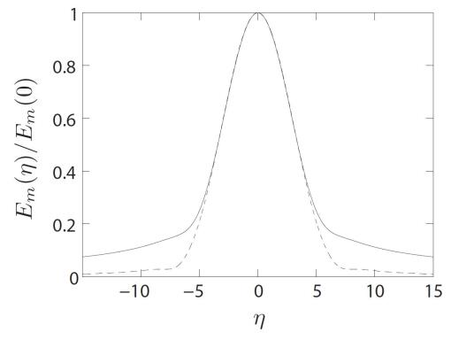
Figure 14: Normalized velocity (—, $m=0$) and vorticity (- -, $m=1$) envelopes of the similarity solutions.

It is interesting to note that velocity and vorticity in the present analysis are analogous to the pressure and velocity in the analysis of Thomas and Stevenson.Thomas1972 One consequence is that the lateral decay of the velocity envelope is sharper for an internal wave (as $1/\eta^{2}$) than for an inertial wave (as $1/\eta$).

Finally, the $z$ component of the velocity is obtained using incompressibility ($\partial_{x}u_{x}+\partial_{z}u_{z}=0$), yielding

$$u_{z}=\frac{1}{3}u_{x}\eta\left(\frac{\ell}{x}\right)^{2/3}=\frac{1}{3}u_{x}\frac{z}{x}.$$ (20)

This result shows that the streamlines projected in the $(x,z)$ plan are along lines of constant phase (i.e., constant $\eta$). As a consequence, a particle trajectory is an approximate circle, projected on curved surfaces, invariant along $y$, and such that $z=\eta^{*}\ell^{2/3}x^{1/3}$, with $\eta^{*}$ given by the initial location.

The thickness $\eta_{1/2}$ of the velocity and vorticity envelopes are defined such that $E_{m}(\eta_{1/2}/2)=E_{m}(0)/2$. Those thicknesses turn out to be almost equal: $\eta_{1/2}\simeq 6.841$ for $m=0$ and $\eta_{1/2}\simeq 6.834$ for $m=1$. In dimensional units, the wave thickness is thus given by Eq. (5). Interestingly, the envelope of $u_{z}$ is given by $\eta E_{0}(\eta)$, which tends towards $1$ as $\eta\rightarrow\infty$, so that no thickness could be defined for $u_{z}$.

Finally, we note that the quasi-parallel approximation used in the present analysis is satisfied for $|u_{z}|/|u_{x}|\ll 1$. Using $|u_{z}|/|u_{x}|=\eta^{1/3}\,(\ell/x)^{1/3}/3$, and evaluating the envelope ratio at the boundary of the wave, i.e., for $\eta=\eta_{1/2}/2\simeq 3.42$, this criterion is satisfied within 10% for $x>38\ell$.

References

- (1) H. Greenspan, “The theory of rotating fluids,” Cambridge University Press (1968).
- (2) J. Lighthill, “Waves in fluids,” Cambridge University Press (1978).
- (3) J. Pedlosky, “Geophysical fluid dynamics,” Springer-Verlag (1987).
- (4) C. Cambon, “Turbulence and vortex structures in rotating and stratified flows,” Eur. J. Mech. B Fluids 20(4), 489–510 (2001).
- (5) O.M. Phillips, “Energy transfer in rotating fluids by reflection of inertial waves,” Phys. Fluids 6(4), 513 (1963).
- (6) D.E. Mowbray and B.S.H. Rarity, “A theoretical and experimental investigation of the phase configuration of internal waves of small amplitude in a density stratified liquid,” J. Fluid Mech. 28, 1–16 (1967).
- (7) N.H. Thomas and T.N. Stevenson, “A similarity solution for viscous internal waves,” J. Fluid Mech. 54 (3), 495–506 (1972).
- (8) B.R. Sutherland, S.B. Dalziel, G.O. Hughes, and P.F. Linden, “Visualization and measurement of internal waves by ‘synthetic Schlieren’. Part 1. Vertically oscillating cylinder,” J. Fluid Mech. 390, 93–126 (1999).
- (9) M.R. Flynn, K. Onu, and B.R. Sutherland, “Internal wave excitation by a vertically oscillating sphere,” J. Fluid Mech. 494, 65 -93 (2003).
- (10) L. Gostiaux, T. Dauxois, H. Didelle, J. Sommeria and S. Viboud, “Quantitative laboratory observations of internal wave reflection on ascending slopes,” Phys Fluids. 18, 056602 (2006).
- (11) L. Gostiaux, H. Didelle, S. Mercier and T. Dauxois, “A novel internal waves generator,” Exp. Fluids 42, 123–130 (2007).
- (12) D. Fultz, “A note on overstability and the elastoid-inertia oscillations of Kelvin, Soldberg, and Bjerknes,” J. Meteo. 16, 199–207 (1959).
- (13) A.D. McEwan, “Inertial oscillations in a rotating fluid cylinder,” J. Fluid Mech. 40, 603–639 (1970).
- (14) R. Manasseh, “Distortions of inertia waves in a rotating fluid cylinder forced near its fundamental mode resonance,” J. Fluid Mech. 265, 345–370 (1994).
- (15) L.R.M. Maas, “Wave focusing and ensuing mean flow due to symmetry breaking in rotating fluids,” J. Fluid Mech. 437, 13–28 (2001).
- (16) P. Meunier, C. Eloy, R. Lagrange and F. Nadal, “A rotating fluid cylinder subject to weak precession,” J. Fluid Mech. 599, 405–440 (2008).
- (17) F.S. Godeferd and L. Lollini, “Direct numerical simulations of turbulence with confinement and rotation,” J. Fluid Mech. 393, 257–308 (1999).
- (18) B. Voisin, “Limit states of internal wave beams,” J. Fluid Mech. 496, 243–293 (2003).
- (19) L. Messio, C. Morize, M. Rabaud and F. Moisy, “Experimental observation using particle image velocimetry of inertial waves in a rotating fluid,” Exp. Fluids 44, 519-528 (2008).
- (20) K.S. Peat, “Internal and inertial waves in a viscous rotating stratified fluid,” Appl. Sci. Res. 33, 481–499 (1978).
- (21) D.G. Hurley and G. Keady, “The generation of internal waves by vibrating elliptic cylinders. Part 2. Approximate viscous solution,” J. Fluid Mech. 351, 119–138 (1997).
- (22) DaVis, LaVision GmbH, Anna-Vandenhoeck-Ring 19, 37081 Goettingen, Germany, complemented with the PIVMat toolbox for Matlab, http://www.fast.u-psud.fr/pivmat
- (23) M.S. Longuet-Higgins, “Mass transport in water waves,” Phil. Trans. Roy. Soc. London. Ser. A. 245, 903, 535–581 (1953).
- (24) A numerical integration of the particle trajectory in the center of the beam () actually shows that the numerical prefactor in Eq. (11) is 1.047 instead of 2/3.